
Statistical Physics Notes 1. Probability Discrete distributions A variable x takes n discrete...
43
Statistical Physics Notes 1. Probability Discrete distributions A variable x takes n discrete values, {x i , i = 1,…, n} (e.g. throwing of a coin or a dice) After N events, we get a distribution, {N 1 , N 2 , …, N n } Probability: Normalization: Markovian assumption: events are independent N N x P i N i Lim ) ( 1 1 ) ( 1 1 n i i n i i N N x P
-
Upload
carlos-sutton -
Category
Documents
-
view
215 -
download
0
Transcript of Statistical Physics Notes 1. Probability Discrete distributions A variable x takes n discrete...
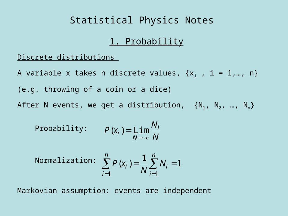
Statistical Physics Notes
1. Probability
Discrete distributions
A variable x takes n discrete values, {xi , i = 1,…, n}
(e.g. throwing of a coin or a dice)
After N events, we get a distribution, {N1, N2, …, Nn}
Probability:
Normalization:
Markovian assumption: events are independent
N
NxP i
Ni
Lim)(
11
)(11
n
ii
n
ii N
NxP

Continuous distributions
A variable x can take any value in a continuous interval [a,b]
(most physical variables; position, velocity, temperature, etc)
Partition the interval into small bins of width dx.
If we measure dN(x) events in the interval [x,x+dx], the probability is
Normalization:
dxdN
NxP
N
1Lim)(
NxdN
dxxPN
)(Lim)(
1)( dxxP

Examples: Uniform probability distribution
Gaussian distribution
A: normalization constant
x0: position of the maximum
: width of the distribution
ax
axaxP
0,0
0,/1)(
98.0
212 22
x
e x
a x
1/a
220 2)()( xxAexP
P(x)
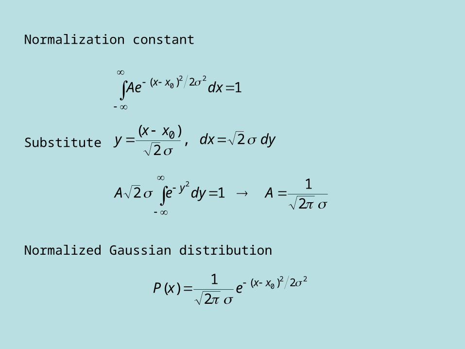
Normalization constant
Substitute
Normalized Gaussian distribution
220 2)(
21
)(
xxexP
21
12
2,2
)(
1
2
220
0
2)(
AdyeA
dydxxx
y
dxAe
y
xx

Properties of distributions
Average (mean)
discrete distribution
continuous distribution
Median (or central) value: 50% split point
Most probable value: P(x) is maximum
For a symmetric distribution all of the above are equal (e.g. Gaussian).
Mean value of discrete
an observable f(x) continuous
dxxxP
xPxx
n
iii
)(
)(1
dxxPxf
xPxff
i ii
)()(
)()(

Variance: measures the spread of a distribution
Root mean square (RMS) or standard deviation:
Same dimension as mean, used in error analysis:
xx )var( dev RMS
22
22
2
2
)()(2)(
)(
)var(
xx
xPxxPxxxPx
xPxx
xxx
i iii i iii
ii i
xx

Examples: Uniform probability distribution, a
Gaussian distribution
For variance, assume
xdyeyx
xydxexxx
y
x
222
222
2
22
2)var(
2,2
1)var( Let
02)( ,
21
)(22
0 xxexP xx
3212)var(,
2,1
)(2 a
xa
xa
xa
xP
0x

Detour: Gaussian integrals
Fundamental integral:
Introduce
nxn
nnbxn
n
n
xbx
xbx
ndxex
b
ndxex
db
Id
dxexb
dxexdb
Id
dxexb
dxexdb
dI
2
!)!12(
2
)12(31
2
31
2
3
22
22
22
22
22/)12(
2
24
2/524
2
2
22/3
2
bdxebI bx
2
)(
dxe x2

Addition and multiplication rules
Addition rule for exclusive events:
Multiplication rule for independent variables x and y
discrete
continuous
Examples: 2D-Gaussian distribution
If dxdye
dxdyeedayxP
yxyx
yx
yxxy
yx
222
2222
2)(2
22
2
1,
2
1),(
jixPxPxxP jiji )()()or(
dyyPdxxPdayxP
yPxPyxP
xy
jiji
)()(),(
)()(),( 21joint

In cylindrical coordinates, this distribution becomes
Since it is independent of , we can integrate it out
Mean and variance
rdrdedarP rr
22 222
1),(
22
22
22
22
)(
22
1)(
rr
rr
er
rP
drredrrP
)22()var(
2
2
2
x
r
r

3D-Gaussian distribution with equal ’s
In spherical coordinates
We can integrate out and
Here r refers to a vector physical variable, e.g. position, velocity, etc.
dddrrerdrP
rderdzyxP
rr
zyxxyz
sin)2(
1),,(
)2(
1),,(
2232/3
3
32)(32/3
3
22
2222
22
22
23
2
2232/3
2)(
4)2(
1)(
rr
rr
er
rP
drredrrP

Mean and variance of 3D-Gaussian distribution
1) gives partsby on(integrati
substitute
82
12
212
0
43
22
0
233
22
duue
rudrerr
u
r
) gives (integral
substitute
833212
212
2
0
452/53
0
243
2
2
22
dyey
rydrerr
y
r
67.045.083)var( 22 rr

Most probable value for a 3D-Gaussian distribution
Set
Summary of the properties of a 3D-Gaussian dist.:
2~2~
02
12
02
22
22
2
22 22
rr
rr
er
rr r
7.13,6.18
,4.12~ 2 rrr
22 23
22)(0
r
rr e
rrP
dr
dP for

Binomial distribution
If the probability of throwing a head is p and tail is q (p+q=1), then the
probability of throwing n heads out of N trials is given by the binomial
distribution:
The powers of p and q in the above equation are self-evident.
The prefactor can be found from combinatorics. An explicit construction
for 1D random walk or tossing of coins is shown in the next page.
nNnqpnNn
NnP
)!(!
!)(

Explicit construction of the binomial distribution
There is only 1 way to get all H or T,
N ways to get 1T and (N-1)H (or vice versa),
N(N-1)/2 ways to get 2T and (N-2)H,
N(N-1)(N-2)…(N-n+1)/n! ways to get nT and (N-n)H (binomial coeff.)
NNNN HTHHTTNLLNLNNLN
HHHTHHTTHTTTLLLL
HHHTTHTTLL
HTLL
HTx
11)1()1(
333
2022
1
/
Trial

Properties of the binomial distribution:
Normalization follows from the binomial theorem
Average value of heads
For
pNqppNqpp
pp
Sp
qpnNn
NnnnPn
NN
N
n
nNnN
n
1
00
)()(
)!(!
!)(
1)()(
)!(!!
)(,
0
0
NN
n
N
n
nNnN
qpnP
qpnNn
NqpqpS
2/,2/1 Nnp

Average position in 1D random walk after N steps
For large N, the probability of getting is actually quite small.
To find the spread, calculate the variance
NpqnqpNpNppNpN
qpNpqppN
qpNpp
pqpp
pSp
p
qpnNn
Nnn
NN
NN
N
n
nNn
2
21
122
0
22
)(1
))(1()(
)()(
)!(!!
2/1,0
)()12(22
qpx
NLqpNLpLNnLNnx
if
0x

Hence the variance is
To find the spread in position, we use
LNx
qpNLxx
NpqLLnnxxx
LNnNnx
LNnNnx
)(
2/1,)var(
44)var(
44
44
22
222222
2222
2222
rms
if
2/1,4/)var(
)var( 22
qpNn
Npqnnn
if
2222 44 LNNnnx

Large N limit of the binomial distribution:
Mean collision times of molecules in liquids are of the order of picosec.
Thus in macroscopic observations, N is a very large number
To find the limiting form of P(n), Taylor expand its log around the mean
Stirling’s formula for ln(n!) for large n,
nn nPdn
dnnnP
dn
dnnnP
qnNpnnNnNnP
)(ln)(2
1)(ln)()(ln
ln)(ln)!ln(!ln!ln)(ln
2
22
nnnndn
d
nnnnn
ln2/111ln!ln
)2ln(ln!ln 21

Substitute the derivatives in the expansion of P(n)
Npqnn
nPnP
NpqnnnPnP
2)(
)()(
ln
1)(
21
)(ln)(ln
2
2
NpqNpqqp
qpNnNnnP
dn
d
qnpn
qnpnn
qnpnN
qpnNnnPdnd
qnNpnnNnNnP
n
n
111111)(ln
01ln)1(
ln)(
ln)(
ln
lnln)ln(ln)(ln
ln)(ln)!ln(!ln!ln)(ln
2
2

Thus the large N limit of the binomial distribution is the Gaussian dist.
Here is the mean value, and the width and normalization are
For the position variable we have
NpqnnenPnP 2)( 2
)()(
NpqnPNpq
2
1
2
1)(,
NLqpNLpLNnx
exP
LNpqLnnxx
xxx
x
x
)()12()2(
21
)(
2,2)(
22 2)(
,)2( LNnx
Npn
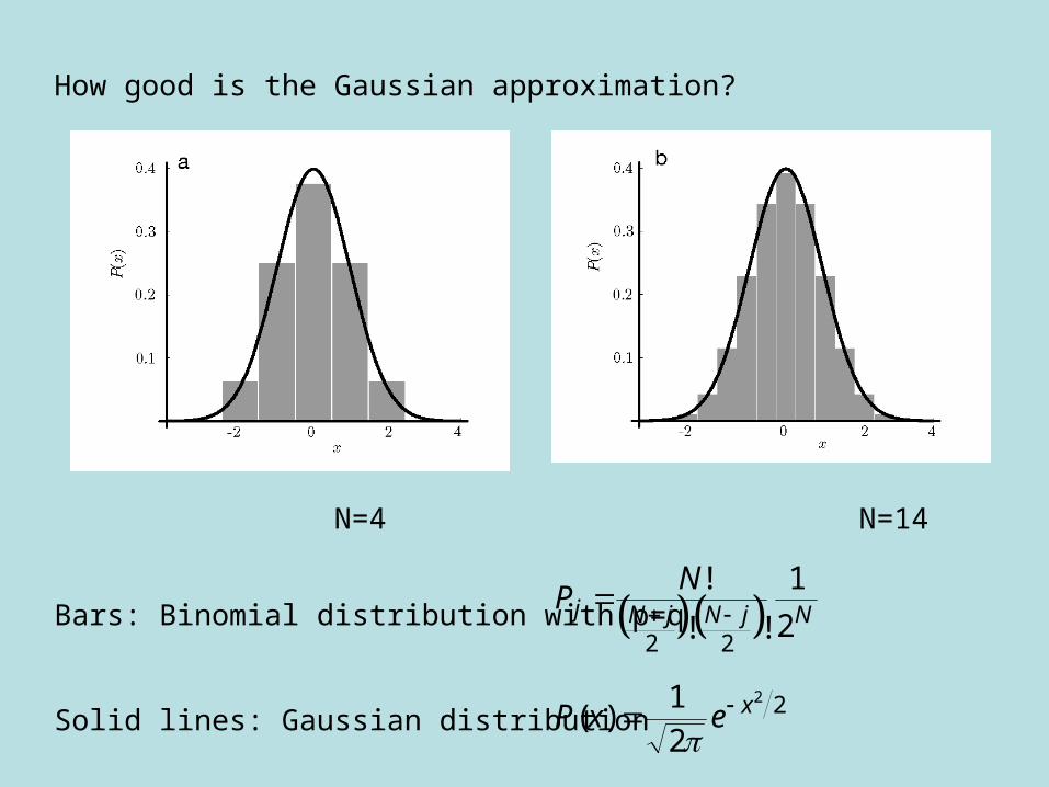
How good is the Gaussian approximation?
N=4 N=14
Bars: Binomial distribution with p=q
Solid lines: Gaussian distribution
2
22
2
21
)(
2
1
!!
!
x
NjNjNj
exP
NP

2. Thermal motion
Ideal gas law:
Macroscopic observables:
P: pressure, V: volume, T: temperature
N: number of molecules
k = 1.38 x 10⁻²³ J/K (Boltzmann constant)
At room temperature (Tr = 298 K), kTr = 4.1 x 10⁻²¹ J = 4.1 pN nm
(kTr provides a convenient energy scale for biomolecular system)
The combination NkT suggests that the kinetic energy of individual
molecules is about kT. To link the macroscopic properties to molecular
ones, we need an estimate of pressure at the molecular level.
NkTPV

Derivation of the average kinetic energy from the ideal gas law
Consider a cubic box of length L filled with N gas molecules
The pressure on the walls arises from the collision of molecules
Momentum transfer to the y-z wall
Average collision time
Force on the wall due a single coll.L
mv
vL
mv
tq
f
vLt
mvmvmvq
x
x
xx
x
xxx
2
2
2
2
2)(

In general, velocities have a distribution, so we take an average
Average force due to one molec.
Average force due to N molec’s
Pressure on the wall
Generalise to all walls
Average kinetic energy
Equipartition thm.: Mean energy associated with each deg. of fredom is:
kTvmK
kTvmvmvmN
PV
vmV
Nv
AL
Nm
A
FP
vL
NmfNF
vL
mf
zyx
xxx
xxx
xx
2
3
2
1 2
222
22
2
2
kT21

Distribution of speeds
Experimentalset up
Experimental results for Tl atoms
○ T=944 K
● T=870 K
▬▬ 3D-Gaussian dist.
v is reduced by
Velocity filter
mkTv /2~
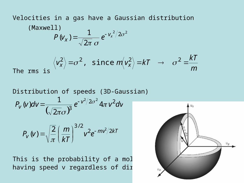
Velocities in a gas have a Gaussian distribution (Maxwell)
The rms is
Distribution of speeds (3D-Gaussian)
This is the probability of a molecule having speed v regardless of direction
mkT
kTvmv
evP
xx
vx
x
2222
2
,
21
)(22
since
kTmvv
vv
evkT
mvP
dvvedvvP
222/3
223
2
22
2)(
42
1)(

Example: the most common gas molecule N2
Oxygen is 16/14 times heavier, so for the O2 molecule, scale the above
results by
Hydrogen is 14 times lighter, so for H2 scale the above results by
m/s
m/s
m/s
m/s
5103
4708
4202~
300107.4
101.4
2
26
21
v
v
v
mkT
94.08/7
7.314

Generalise the Maxwell distribution to N molecules
(Use the multiplication rule, assuming they move independently)
This is simply the Boltzmann distribution for non-interacting N particles.
In general, the particles interact so there is also position dependence:
Universality of the Gaussian dist. arises from the quadratic nature of E.
kTE
kTm
kTmkTmkTmN
e
e
eeeP
N
N
kin
2),,(
22221
222
21
222
21),,,(
vvv
vvvvvv
),,,,,,(
),,,,,,(
2211
/2211
NN
kTENN
EEEE
eP
vrvrvr
vrvrvr
potkintot
tot

Activation barriers and relaxation to equilibrium
Speed dist. for boiling water at 2 different temperatures
Removing the most energetic molecules creates a non-equilibrium state.
When boiled, water molecules with sufficient kinetic energy evaporate
Arrhenius rate law: Ebarrier : Activation barrier
Those molecules with K.E. > Ebarrier can escape
kTEe /barrier

Equilibrium state (i.e. Gaussian dist.) is restored via molecular collisions
Injecting very fast molecules
in a box of molecules results
in an initial spike in the
Gaussian distribution
Gas molecules collide like billiard balls
(Energy and momentum are conserved)
Thus in each collision, the fast molecules
lose energy to the slower ones (friction)

3. Entropy, Temperature and Free Energy
Entropy is a measure of disorder in a closed system.
When a system goes from an ordered to a disordered state, entropy
increases and information is lost. The two quantities are intimately
linked, and sometimes it is easier to understand information loss or gain.
Consider any of the following 2-state system
• Tossing of N coins
• Random walk in 1-D (N steps)
• Box of N gas molecules divided into 2 parts
• N spin ½ particles with magnetic moment in a magnetic field B
Each of these systems can be described by a binomial distribution
NNNppppNNN
NNP NN 21212121
21 ,1,!!
!),( 21

There are 2N states in total, but only N+1 are distinct.
Introduce the number of states with a given (N1, N2) as
We define the disorder (or information content) as
For the 2-state system, assuming large N, we obtain
44.12ln1,ln KKI
)(ln)()(ln)(
)(ln)(ln
lnlnln
!ln!ln!ln
2211
2211
222111
21
NNNNNNNNKNI
NNNNNNK
NNNNNNNNNK
NNNKI
!!!
),(21
21 NNN
NN
(Shannon’s formula)

Thus the amount of disorder per event is
I vanishes for either p1=1 or p2=1 (zero disorder, max info) and
It is maximum for p1=p2=1/2 (max disorder, min info)
Generalization to m-levels:
Max disorder when all pi are equal, and zero disorder when one is 1.
m
i iii i
mm
Nm
NN
mm
ppKNINNKI
NNNN
NNN
pppNNN
NNNNP m
1
2121
2121
21
lnln!lnln
!!!!
),,(
!!!!
),,( 21
2211 lnln ppppKNI
NNp iiii ,1

Entropy
Statistical postulate: An isolated system evolves to thermal equilibrium.
Equilibrium is attained when the probability dist. of microstates has the
maximum disorder (i.e. entropy).
Entropy of a physical system is defined as
Entropy of an ideal gas
2/1
1
3
1
2
1
3
1
2
1
2
1
2
2
21
21
21
N
i kik
N
i kik
N
ii
N
ii
pmE
pm
pm
mvE
),,(ln NEkS
Total energy:
Radius of the sphere in 3N dimensions

Area of such a sphere is proportional to r3N-1 ≈ r3N
Hence the area of the 3N-D volume in momentum space is (2mE)3N/2
The number of allowed states is given by the phase space integral
N
N
NN
NN
NN
hNNC
constVENk
mECVkS
mEV
pdpdrdrd
3
2/3
2/3
2/3
2/3
31
331
3
!2
1
)!12/3(
2
.ln
)2(ln
)2(
Sakure-Tetrode formula
Area of a unit sphere in 3N-D
Planck’s const.

Temperature:
If the energies are not equal, and we allow exchange of energy via
a small membrane, how will the energy evolve? (maximum disorder)
Isolated system
Total energy is conserved
kTN
E
N
E
E
N
E
N
dEdS
VEENVENkES
B
B
A
A
B
B
A
A
A
BABAAAA
23
00
ln)ln(lnln)( 23
23
BA EEE

Example: NA = NB= 10
Fluctuations in energy are proportional to NN
N
E
1

Definition of temperature
At equilibrium:
In general
Free energy of a microscopic system “a” in a thermal bath
BA
BAB
B
A
A
A
TT
TTE
N
E
Nk
dE
dS
0
11
2
3
11
dEdS
TordEdS
T
(zeroth law of thermodynamics)
i
kTE
iiia
aaa
ieZ
EPE
ZkTTSEF ln
Average energy
Partition function

Example: 1D harmonic oscillator in a heat bath
In 3D:
Equipartition of energy: each DOF has kT/2 of energy on average
kTkTkTKm
vxEvxPdxdvE
mkTevP
KkTexP
KxmvvxE
xv
aa
vv
vv
xx
xx
a
v
x
21
212
212
21
2
2
2212
21
),(),(
,2
1)(
,2
1)(
),(
22
22
kTkTkTKmEa 323
232
212
21 rv

Free energy of the harmonic oscillator
Free energy:
Entropy:
kTmmkTkT
h
edpedxh
edxdph
Z
pxpx
pxkTpxE pxa
,21
11
2
22),(2222
kTk
kTkT
TT
FS
kTkFE
TS
kTkTZkTF
aa
aaa
a
ln1ln
ln11
lnln
222
21
21
),( xmpm
pxEa

Harmonic oscillator in quantum mechanics
Energy levels
Free energy:
Entropy:
kT
kT
n
nkT
n
nkT
n
kTn
e
e
xxexxe
eZ
1
1
1,,
2
00
2
0
21
kTkT
kTa
a
kTa
ee
e
kTk
T
FS
ekTZkTF
1ln1
1lnln 21
21 nEn

To calculate the average energy let
Using <Ea> yields the same entropy expression.
Classical limit:
kTke
e
ekT
kS
kTkTekTF
kTE
kTkT
kT
a
kTa
a
ln11ln1
ln1ln21
1, kT
e
e
e
eZ
ZZ
eZ
eEZ
Ei
Ei
Eia
ii
1
121
1
111
2
kT1


![Lecture Notes on Discrete-Time Signal Processingkilyos.ee.bilkent.edu.tr/~ee424/EE424.pdf · Lecture Notes on Discrete-Time Signal Processing ... signal: x[n]=x c(nT s); ... is a](https://static.fdocuments.us/doc/165x107/5a9d9e777f8b9a28388c5cde/lecture-notes-on-discrete-time-signal-ee424ee424pdflecture-notes-on-discrete-time.jpg)