Statistical Models of Temperature in the Sacramento–SanJoaquin Delta Under Climate-Change Scenariosand Ecological Implications

R. Wayne Wagner & Mark Stacey & Larry R. Brown &

Michael Dettinger

Received: 24 September 2009 /Revised: 15 October 2010 /Accepted: 17 December 2010 /Published online: 1 February 2011# The Author(s) 2011. This article is published with open access at Springerlink.com

Abstract Changes in water temperatures caused by climatechange in California’s Sacramento–San Joaquin Delta willaffect the ecosystem through physiological rates of fishesand invertebrates. This study presents statistical models thatcan be used to forecast water temperature within the Deltaas a response to atmospheric conditions. The daily averagemodel performed well (R2 values greater than 0.93 duringverification periods) for all stations within the Delta andSan Francisco Bay provided there was at least 1 year ofcalibration data. To provide long-term projections of Deltawater temperature, we forced the model with downscaleddata from climate scenarios. Based on these projections, theecological implications for the delta smelt, a key species,

were assessed based on temperature thresholds. The modelforecasts increases in the number of days above temper-atures causing high mortality (especially along the Sacra-mento River) and a shift in thermal conditions for spawningto earlier in the year.

Keywords Climate change . Temperature model .

Delta smelt

Introduction

In freshwater and near-coastal marine ecosystems, watertemperatures provide an important constraint on ecologicalfunction (Coutant 1976). Examples include effects on fishspawning (Hotta et al. 2001), swimming performance(Myrick and Cech 2000), metabolism (Das et al. 2005;Scheller et al. 1999), and mortality (Coutant 1976; Johnsonand Evans 1996) as well as effects on aquatic invertebrates(Vannote and Sweeney 1980; Ward and Stanford 1982).Specific examples of species of concern within theSacramento–San Joaquin Delta that are sensitive to watertemperatures at various points in the life cycles include theSacramento winter run Chinook salmon Oncorhynchustshawytscha (Baker et al. 1995), the Sacramento splittailPogonichthys macrolepidotus (Moyle et al. 2004), and thedelta smelt Hypomesus transpacificus (Bennett 2005;Swanson et al. 2000).

Climate change is projected to result in increases inmean annual air temperature of 2.2–5.8°C in the comingcentury averaged across the state of California (Loarie et al.2008). An increase in air temperature will lead to earliersnowmelt, more precipitation falling as rain (vs. snow), andchanges in the operation of California’s water deliverysystem (Barnett et al. 2008; Vanrheenen et al. 2004). To

R. W. Wagner (*)Department of Civil and Environmental Engineering,University of California, Berkeley,205 O’Brien Hall, Mail Code 1712,Berkeley, CA 94720-1720, USAe-mail: wagnerw@berkeley.edu

M. StaceyDepartment of Civil and Environmental Engineering,University of California, Berkeley,665 Davis Hall, Mail Code 1710,Berkeley, CA 94720-1710, USAe-mail: mstacey@berkeley.edu

L. R. BrownU.S. Geological Survey,Placer Hall, 6000 J Street,Sacramento, CA 95819-6129, USAe-mail: lrbrown@usgs.gov

M. DettingerU.S. Geological Survey, UC San Diego,Scripps Institute of Oceanography, 9500 Gilman Drive,La Jolla, CA 92093-0224, USAe-mail: mddettin@usgs.gov

Estuaries and Coasts (2011) 34:544–556DOI 10.1007/s12237-010-9369-z

analyze the effects of climate change on fish populations,however, we require projections of water temperature underglobal warming scenarios.

In tidal systems, the water temperature at a particularlocation is determined by the interplay between atmospher-ic forcing, tidal dispersion, and riverine flows (Monismithet al. 2009). Formal models of tidal dispersion are notcurrently feasible for projections of temperature overcenturies given the magnitude of the computational require-ments. In view of this limitation, we have developed astatistical model of temperature in the Sacramento–SanJoaquin Delta. Our emphasis in this paper is on under-standing the dynamics of water temperatures and theirpossible effects on aquatic species.

Study Location

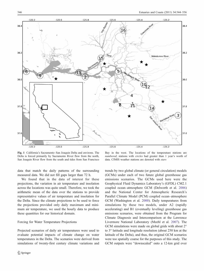
This study focuses on California’s Sacramento–San JoaquinDelta (the Delta) and nearby environs, which are located atthe upstream end of the San Francisco Estuary. Detaileddescriptions of the Delta can be found in Kimmerer (2004)and Lund et al. (2007). It consists of a network of channels(Fig. 1) that are fed by freshwater flow from a number ofrivers that drain California’s Central Valley, mostsignificantly the Sacramento and San Joaquin Rivers(Kimmerer 2004). The Delta serves as the hub ofCalifornia’s water system, draining roughly 45% of thestate’s area (Lund et al. 2007) and providing water supplyto approximately two thirds of its population. In itsunaltered state, the Delta was a system of sloughs andmarshlands (both of which were open to influence fromriver flows and tidal effects), but currently it is a system ofleveed, subsided farmlands separated by channelized tidalsloughs and rivers (Kimmerer 2004).

California’s water distribution system relies heavily onthe Delta because reservoir releases must move through theDelta on their way to pumping stations for delivery to waterusers throughout the state (Lund et al. 2007). The mostimportant of these stations are located in the southern Deltaand provide water for the Delta Mendota Canal and theCalifornia Aqueduct, both of which carry water tomunicipal and agricultural users south of the Delta(Kimmerer 2004). The levees, dams, and diversions havedrastically altered the hydrologic system from its nativestate. The ecology of the delta has been similarly altered, asit has responded to the changing hydrology as well asintroductions of non-native fish, clams, and aquatic plants(Kimmerer 2004). Climate change will impact the Delta ina number of ways; examples include hydrologic change asthe proportion of precipitation falling as snow declines inthe Sierra Nevada mountain range (Vanrheenen et al. 2004),local heat budget adjustment to a warmer atmosphere, andestuarine response to sea level rise.

Data

Measured Water Temperature Data

We downloaded time series of measured water temperaturesfrom the Interagency Ecological Program (http://www.iep.ca.gov), which receives the data from the CaliforniaDepartment of Water Resources, the United States GeologicSurvey, the California Data Exchange Center, and theUnited States Bureau of Reclamation, for locationsthroughout the Delta (Fig. 1). For many stations, watertemperature data collection started in the mid-1980s andextends to the current time. The data have been collected ateither 15-min intervals or hourly. For consistency amongthe data sets, we averaged the 15-min data to give hourlydatasets. To handle outliers, we deleted all points outside 4standard deviations from the mean of 20-h windows of thedata. At locations where two or more agencies collecteddata, we averaged the data to create one dataset for eachlocation. We calculated the daily maximum, average, andminimum water temperatures from these data for modelcalibration and verification.

Measured Forcing Data

We downloaded hourly air temperatures and insolationfrom the California Irrigation Management InformationSystem (CIMIS; http://www.cimis.water.ca.gov) at sevenlocations within the Delta (Fig. 1; stations were Lodi,Brentwood, Manteca, Twitchell Island, Lodi West, Tracy,and Concord). We downloaded an additional six airtemperature locations from the Interagency EcologicalProgram (locations 2, 9, 10, 13, 14, and 15 on Fig. 1). Asan initial processing step, we removed physically impossi-ble values (air temperatures less than −5°C or greater than45°C; insolation less than 0 W/m2 or greater than the solarconstant (1,368 W/m2; Rubin and Davidson 2001)) fromboth datasets.

To handle outliers in the air temperature data, we deletedall points outside 4 standard deviations from the mean of20-h windows of the data. Model verification requirescontinuous forcing because the model output depends onthe output from the previous time step. For this reason andfor verification use only, we created a second air temper-ature dataset wherein gaps in the data shorter than 72 hwere filled. We filled small gaps (<6 h) in this seconddataset through linear interpolation. We filled longer gaps(<72 h) by first linearly interpolating and then adding adiurnal pattern defined by the diurnal cycles duringadjacent (within 1 week) time periods spanning the sametime of day as the gap. The daily cycle was defined by anaverage based on the time of day and was then added to thelinear interpolation of the gap itself to produce synthetic

Estuaries and Coasts (2011) 34:544–556 545

data that match the daily patterns of the surroundingmeasured data. We did not fill gaps larger than 72 h.

We found that in the data of interest for theseprojections, the variation in air temperature and insolationacross the locations was quite small. Therefore, we took thearithmetic mean of the data over the stations to providerepresentative values of air temperature and insolation forthe Delta. Since the climate projections to be used to forcethe projections provided only daily maximum and mini-mum air temperature, we used the hourly data to producethese quantities for our historical domain.

Forcing for Water Temperature Projections

Projected scenarios of daily air temperatures were used toevaluate potential impacts of climate change on watertemperatures in the Delta. The scenarios were derived fromsimulations of twenty-first century climate variations and

trends by two global climate (or general circulation) models(GCMs) under each of two future global greenhouse gasemissions scenarios. The GCMs used here were theGeophysical Fluid Dynamics Laboratory’s (GFDL) CM2.1coupled ocean–atmosphere GCM (Delworth et al. 2006)and the National Center for Atmospheric Research’sParallel Climate Model (PCM) coupled ocean–atmosphereGCM (Washington et al. 2000). Daily temperatures fromsimulations by these two models, under A2 (rapidlyaccelerating) and B1 (eventually leveling) greenhouse gasemissions scenarios, were obtained from the Program forClimate Diagnosis and Intercomparison at the LawrenceLivermore National Laboratory (Meehl et al. 2007). TheGCM simulations were made on global grids with about 2°to 3° latitude and longitude resolution (about 250 km at thelatitude of the Delta), and thus, the original GCM scenarioswere too spatially coarse for the purposes of this study. TheGCM outputs were “downscaled” onto a 12-km grid over

Fig. 1 California’s Sacramento–San Joaquin Delta and environs. TheDelta is forced primarily by Sacramento River flow from the north,San Joaquin River flow from the south and tides from San Francisco

Bay in the west. The locations of the temperature stations arenumbered; stations with circles had greater than 1 year’s worth ofdata. CIMIS weather stations are denoted with stars

546 Estuaries and Coasts (2011) 34:544–556

the conterminous USA by a method called constructedanalogs (Hidalgo et al. 2008). This statistical downscalingmethod is applied to each day’s simulated climate conditionin turn and is based on fitting a linear combination ofhistorical weather patterns (aggregated onto the GCM grid)that best reproduces the GCM pattern for the day. Thecoefficients necessary to make this linear fit are thenapplied to high-resolution versions of the weather on thesame historical days. This approach ensures that, day byday, the weather simulated by the GCM is faithfully carrieddown to the 12-km scale and tends to yield particularlyrealistic temperature relations across areas with sharpgeographic gradients (Cayan et al. 2009). When applied tothe historical record, as a validation exercise, the methodreproduces daily temperature variations quite accurately onthe 12-km grid given only historical temperatures asobserved on the GCM grids as inputs (Hidalgo et al.2008), indicating that the downscaled future-climate pat-terns are likely to also be realistic. The method was appliedto climate simulations spanning the period from 1950 to2100, to obtain daily, gridded temperature patterns oftwenty-first century warming over California and the Delta.

The air temperature data were sub-sampled for the Deltaregion and then averaged to produce an equivalent forcingtime series for 2000 though 2100 to those used during thecalibration/verification stage. The data from the scenariosincluded maximum and minimum daily air temperatures.The climate projections did not provide insolation, so wederived the average insolation based on Julian day of theyear. We extended this dataset to create a 100-year recordunder the assumption that insolation will be relativelyconstant over these climatic time scales.

Data Analysis

Temporal Variability

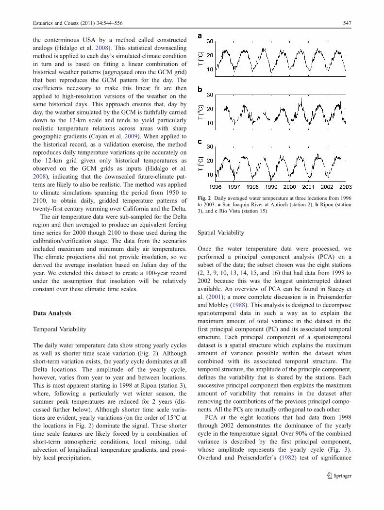
The daily water temperature data show strong yearly cyclesas well as shorter time scale variation (Fig. 2). Althoughshort-term variation exists, the yearly cycle dominates at allDelta locations. The amplitude of the yearly cycle,however, varies from year to year and between locations.This is most apparent starting in 1998 at Ripon (station 3),where, following a particularly wet winter season, thesummer peak temperatures are reduced for 2 years (dis-cussed further below). Although shorter time scale varia-tions are evident, yearly variations (on the order of 15°C atthe locations in Fig. 2) dominate the signal. These shortertime scale features are likely forced by a combination ofshort-term atmospheric conditions, local mixing, tidaladvection of longitudinal temperature gradients, and possi-bly local precipitation.

Spatial Variability

Once the water temperature data were processed, weperformed a principal component analysis (PCA) on asubset of the data; the subset chosen was the eight stations(2, 3, 9, 10, 13, 14, 15, and 16) that had data from 1998 to2002 because this was the longest uninterrupted datasetavailable. An overview of PCA can be found in Stacey etal. (2001); a more complete discussion is in Preisendorferand Mobley (1988). This analysis is designed to decomposespatiotemporal data in such a way as to explain themaximum amount of total variance in the dataset in thefirst principal component (PC) and its associated temporalstructure. Each principal component of a spatiotemporaldataset is a spatial structure which explains the maximumamount of variance possible within the dataset whencombined with its associated temporal structure. Thetemporal structure, the amplitude of the principle component,defines the variability that is shared by the stations. Eachsuccessive principal component then explains the maximumamount of variability that remains in the dataset afterremoving the contributions of the previous principal compo-nents. All the PCs are mutually orthogonal to each other.

PCA at the eight locations that had data from 1998through 2002 demonstrates the dominance of the yearlycycle in the temperature signal. Over 90% of the combinedvariance is described by the first principal component,whose amplitude represents the yearly cycle (Fig. 3).Overland and Preisendorfer’s (1982) test of significance

Fig. 2 Daily averaged water temperature at three locations from 1996to 2003: a San Joaquin River at Antioch (station 2), b Ripon (station3), and c Rio Vista (station 15)

Estuaries and Coasts (2011) 34:544–556 547

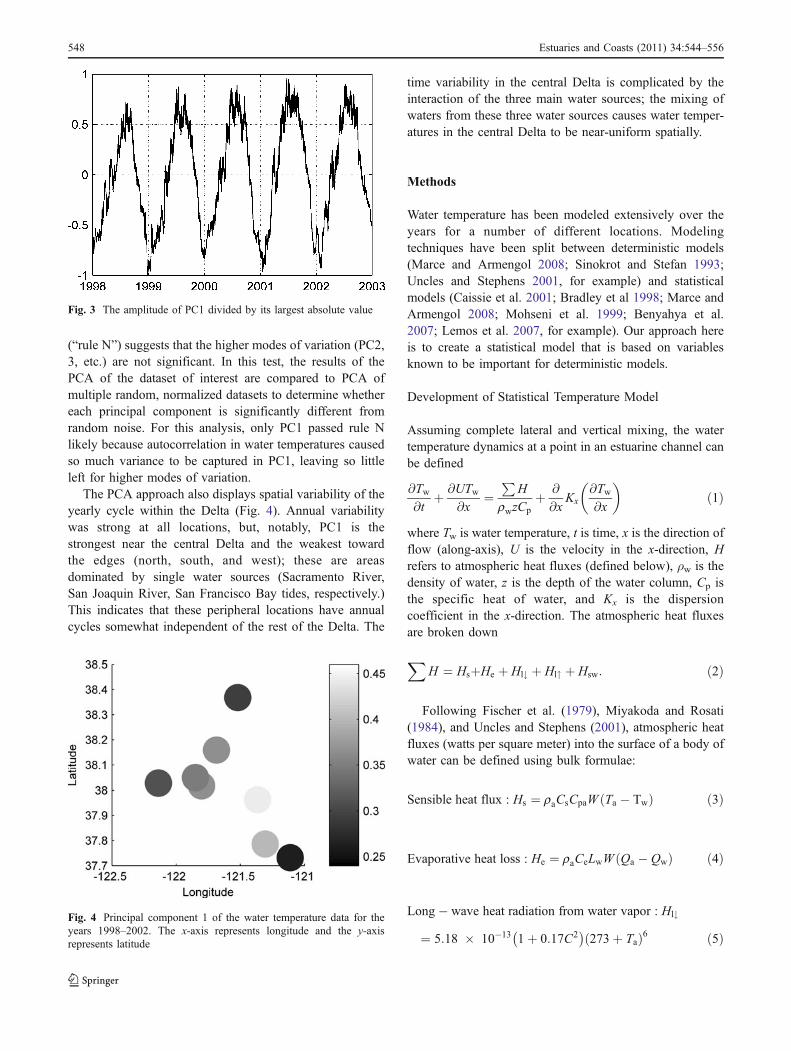
(“rule N”) suggests that the higher modes of variation (PC2,3, etc.) are not significant. In this test, the results of thePCA of the dataset of interest are compared to PCA ofmultiple random, normalized datasets to determine whethereach principal component is significantly different fromrandom noise. For this analysis, only PC1 passed rule Nlikely because autocorrelation in water temperatures causedso much variance to be captured in PC1, leaving so littleleft for higher modes of variation.

The PCA approach also displays spatial variability of theyearly cycle within the Delta (Fig. 4). Annual variabilitywas strong at all locations, but, notably, PC1 is thestrongest near the central Delta and the weakest towardthe edges (north, south, and west); these are areasdominated by single water sources (Sacramento River,San Joaquin River, San Francisco Bay tides, respectively.)This indicates that these peripheral locations have annualcycles somewhat independent of the rest of the Delta. The

time variability in the central Delta is complicated by theinteraction of the three main water sources; the mixing ofwaters from these three water sources causes water temper-atures in the central Delta to be near-uniform spatially.

Methods

Water temperature has been modeled extensively over theyears for a number of different locations. Modelingtechniques have been split between deterministic models(Marce and Armengol 2008; Sinokrot and Stefan 1993;Uncles and Stephens 2001, for example) and statisticalmodels (Caissie et al. 2001; Bradley et al 1998; Marce andArmengol 2008; Mohseni et al. 1999; Benyahya et al.2007; Lemos et al. 2007, for example). Our approach hereis to create a statistical model that is based on variablesknown to be important for deterministic models.

Development of Statistical Temperature Model

Assuming complete lateral and vertical mixing, the watertemperature dynamics at a point in an estuarine channel canbe defined

@Tw@t

þ @UTw@x

¼P

H

rwzCpþ @

@xKx

@Tw@x

� �

ð1Þ

where Tw is water temperature, t is time, x is the direction offlow (along-axis), U is the velocity in the x-direction, Hrefers to atmospheric heat fluxes (defined below), ρw is thedensity of water, z is the depth of the water column, Cp isthe specific heat of water, and Kx is the dispersioncoefficient in the x-direction. The atmospheric heat fluxesare broken down

XH ¼ HsþHe þ Hl# þ Hl" þ Hsw: ð2Þ

Following Fischer et al. (1979), Miyakoda and Rosati(1984), and Uncles and Stephens (2001), atmospheric heatfluxes (watts per square meter) into the surface of a body ofwater can be defined using bulk formulae:

Sensible heat flux : Hs ¼ raCsCpaW Ta � Twð Þ ð3Þ

Evaporative heat loss : He ¼ raCeLwW Qa � Qwð Þ ð4Þ

Long� wave heat radiation from water vapor : Hl#

¼ 5:18 � 10�13 1þ 0:17C2� �

273þ Tað Þ6 ð5ÞFig. 4 Principal component 1 of the water temperature data for theyears 1998–2002. The x-axis represents longitude and the y-axisrepresents latitude

Fig. 3 The amplitude of PC1 divided by its largest absolute value

548 Estuaries and Coasts (2011) 34:544–556

Long� wave heat loss from the water surface : Hl"

¼ �5:23 � 10�8 273þ Twð Þ4 ð6Þ

Short� wave radiation from insolation : Hsw

¼ R 1� að Þ ð7ÞFor all heat fluxes, heating of the water column is

represented by positive signs and cooling by negative. Thesymbols are defined as follows:

α Albedo (dimensionless)C Fractional cloud cover (dimensionless)Ce Empirical exchange coefficient (∼1.5×10−3;

dimensionless)Cs Empirical exchange coefficient (∼1.5×10−3;

dimensionless)Cpa The specific heat of air (1.012×103 J/kg °C)Lw Latent heat of evaporation (2.4×106 J/kg)ρa The density of air (∼1.2 kg/m3)R Insolation (W/m2)Qa Atmospheric mixing ratio (see Fischer et al. 1979;

dimensionless)Qw Saturation mixing ratio at the ocean surface for Tw

(dimensionless)Ta Air temperature (°C)Tw Water temperature (°C)W Wind speed at 10 m (m/s)

Typical values of calculated atmospheric heat fluxeswithin the Delta (Table 1) show the dominance of the long-wave and short-wave radiation terms. Bartholow (1989)observed that river water temperatures are typically notinfluenced by reservoirs more than 25–30 km upstream.This suggests that longitudinal gradients in water temper-ature are likely to be small and contributions from termsdependent on this gradient (advection and diffusion) aresmall by the time a water parcel reaches the Delta. Thus,combining Eqs. 1 and 2 and eliminating terms, we canwrite:

dTwdT

ffi Hl# þ Hl" þ Hsw

rwzCpð8Þ

Or simplified even further:

dTwdT

ffi f Ta; Tw;Rð Þ ð9Þ

Equation 9 could be discretized as

TðtÞ ffi T t � $tð Þ þ $t f Ta;T ;Rð Þð Þ; ð10Þwhere T represents modeled water temperature; we drop thesubscript w in order to emphasize that the model’s predictedwater temperature will depend on the model’s output fromthe previous time step and not on measured values.Equation 10, although deterministic, is the basis for ourstatistical model. Based on the historical water temperaturedata, we applied a simple regression to relate the day’s watertemperature to the air temperature and insolation from thesame day and water temperature from the day preceding it:

TðnÞ ¼ aTaðnÞ þ bT n� 1ð Þ þ cRðnÞ þ d ð11Þwhere n is the day on which the temperature is beingcalculated, a is the coefficient on the current day’s airtemperature, b is the coefficient on the previous days watertemperature, c is the coefficient on the current day’sinsolation, and d is a constant offset. This model can beused to model maximum, minimum, or average watertemperatures. The insolation, R, used was the averageinsolation for each Julian day of the year.

We used our regression model to accurately reconstructhistorical water temperatures with a minimal amount ofdata needs or computational cost. To verify the model, wecalculated regression coefficients for Eq. 11 using the firsthalf of the dataset (the calibration period), then used thesecoefficients to force the model during the entire dataset(both calibration and verification periods). To project watertemperatures for the coming century, we calibrated with theentire historical dataset and forced with the downscaledclimate data and the annual insolation cycle.

Performance Metrics

We measured model performance through the root meansquared error (RMSE), the coefficient of determination(R2), and the Nash–Sutcliffe coefficient (NSC). The firstgives an idea of the magnitude of the errors. The latter twoquantify how well the model performed on the whole.

The final metric, the Nash–Sutcliffe coefficient, has beenused widely to evaluate the performance of hydrologicmodels and is defined (Nash and Sutcliffe 1970) as

NSC ¼ 1�P

Ni¼1 Oi � Pið Þ2

PNi¼1 Oi � Oð Þ2 ; ð12Þ

where O represents observed data with N realizations and Prepresents predicted data. Values of NSC range from −∞ to

Table 1 Typical values for the surface heat fluxes into (+) and out of(−) the water column for Stockton Ship Canal at Burns Cutoff (station10)

Stockton–Manteca

Month Hs He Hl" Hl# Hsw ∑H

January −3.5 −9.3 −331.0 270.6 55.0 −18.3August −12.0 −102.3 −416.4 346.8 277.0 93.1

Estuaries and Coasts (2011) 34:544–556 549

1.0. Higher values indicate better agreement. A value ofzero indicates that the predicted values are no better thanthe mean of the observations as a predictor; negative valuesindicate that the observed mean is a better predictor. TheNSC has been criticized as a metric because it (like R2)gives too much weight to outliers. Additionally, Garrick etal. (1978) have argued that it is possible to get high valuesfor the NSC with poor models while good models do notscore much higher.

Results

Calibration and Verification of Statistical TemperatureModel

Figure 5 presents time series of the calibration andverification periods from a long-term record on the SanJoaquin River at Antioch (station 2). The annual cycle isclearly well-predicted, as are shorter time scale variations,particularly weekly to monthly fluctuations. A moredifficult test is shown in Fig. 6, for which temperature datawere only collected during the spring at San Joaquin Riverat Prisoner’s Point (station 5); the model was still able tocapture the annual cycle sampled at the end of theverification period. This is most likely because the rangeof the data was close to the annual range in temperature.

The model performed very well at locations where morethan 1 year of data were available for calibration. Afterlocations with less than 1 year of data were removed, themodel fit the data well (Table 2) with R2 values greater than

0.930 (and generally over 0.965) and NSC values greaterthan 0.890 (and generally over 0.950) for verificationperiods for all locations except Ripon (station 3), which ison the Stanislaus River and farther from tidal influence thanthe other stations.

Projections of Water Temperatures for Climate Scenarios

Model projections predict long-term changes in watertemperatures throughout the Delta (model coefficients arereported in Table 3). Figure 7 shows an example of theseprojections, showing projected water temperatures on theSan Joaquin River at Antioch (station 2) under PCM A2forcing. In this particular case, both the yearly high andlow water temperatures increase over the 100-year timehorizon.

Discussion

Model Limitations

One major concern is the ability of a statistical model toproject water temperatures in a changing system. Themodel predicts the seasonal cycle as well as capturingmuch of the short-term variability compared to measureddata. These seasonal fluctuations (the dominant mode ofvariability) are much larger than the long-term trendsexpected with climate change. On the other hand, increasesin water temperatures could lead to increases in evaporativecooling and ultimately cause a leveling off of water

Fig. 6 Calibration (a) and verification (b) at San Joaquin River atPrisoner’s Point (station 5). The measured values are indicated withthe solid line; the modeled values are indicated with the gray line.R2 values are 0.976 for calibration and 0.974 for verification

Fig. 5 Calibration (a) and verification (b) at the San Joaquin River atAntioch (station 2). The measured values are indicated with the solidline; the modeled values are indicated with the gray line. Thecalibration R2 was 0.981; verification R2 was 0.978

550 Estuaries and Coasts (2011) 34:544–556

temperatures near some maximum (Mohseni et al. 1999).While this dynamic is not included in the model, the modelis effective at predicting the maximum temperaturescontained in the historical record of the current regime.

While this approach has been successful at reproducingwater temperatures at locations of long-term records, thelocal spatial variability of the system is not captured. Thestatistical approach essentially projects the water tempera-ture that would be measured at the instrumentation site. It isunclear if those temperature measurements are representa-tive of the local or regional water temperature. Dependingon the station and the method of deployment of theinstrument, there are likely to be both lateral and verticalgradients in water temperature that would reduce theapplicability of the results for locations other than theinstrument sites. Further, variation between stations maynot be linear but may change abruptly at channel junctionsor other Delta features. Finally, all of the long-term stations

are located along either the Sacramento or San JoaquinRiver channels, so the applicability of the results to othersloughs and channels in the Delta is unclear.

Flow Effects

The model skill evident in our verification periods indicatesthat riverine flows are not required to effectively predictwater temperatures in the Delta on long time scales.However, on shorter time scales, large flows create featuresthat the model is unable to accurately forecast.

Although flow effects on water temperatures are, to greatextent, overwhelmed by atmospheric influences, flow doesappear to have significant effects over shorter time scales, andsome events have longer-term implications. We performed aPCA on each year from 1998 to 2002 individually to evaluatethe inter-year stability of the annual cycle. The comparison ofthe first PC (the yearly cycle) for these years (Fig. 8) shows a

Station RMSE−Cal (°C) RMSE−Ver (°C) R2−Cal R2−Ver NSC−Cal NSC−Ver

2 Tmax 0.74 0.78 0.98 0.97 0.98 0.97

T 0.66 0.70 0.98 0.98 0.98 0.98

Tmin 0.67 0.71 0.98 0.98 0.98 0.98

3 Tmax 1.88 2.06 0.79 0.89 0.79 0.80

T 1.74 1.90 0.79 0.89 0.79 0.80

Tmin 1.63 1.52 0.78 0.92 0.78 0.85

5 Tmax 0.65 1.42 0.97 0.93 0.97 0.89

T 0.65 0.90 0.97 0.98 0.97 0.95

Tmin 0.64 0.98 0.97 0.97 0.97 0.94

6 Tmax 0.68 0.77 0.97 0.97 0.97 0.96

T 0.63 0.69 0.98 0.97 0.98 0.97

Tmin 0.63 0.70 0.97 0.97 0.97 0.97

9 Tmax 0.85 0.89 0.96 0.96 0.96 0.96

T 0.75 0.73 0.97 0.97 0.97 0.97

Tmin 0.72 0.77 0.97 0.96 0.97 0.96

10 Tmax 1.17 1.00 0.96 0.97 0.96 0.97

T 1.17 1.00 0.96 0.97 0.96 0.97

Tmin 1.18 1.04 0.96 0.97 0.96 0.97

13 Tmax 1.36 0.97 0.91 0.96 0.91 0.96

T 1.08 0.75 0.94 0.97 0.94 0.97

Tmin 1.01 0.85 0.95 0.96 0.95 0.96

14 Tmax 1.21 1.23 0.96 0.95 0.96 0.95

T 1.20 1.22 0.95 0.95 0.95 0.95

Tmin 1.20 1.23 0.95 0.95 0.95 0.95

15 Tmax 0.92 0.93 0.97 0.97 0.97 0.96

T 0.94 0.94 0.97 0.96 0.97 0.96

Tmin 0.94 0.96 0.97 0.96 0.97 0.96

16 Tmax 0.86 1.13 0.97 0.97 0.97 0.96

T 0.84 1.10 0.97 0.97 0.97 0.96

Tmin 0.83 1.09 0.97 0.97 0.97 0.96

Table 2 This table lists calcu-lated performance metrics foreach variable with at least 1 yearof calibration data for bothcalibration and verification peri-ods. Cal calibration, Ver verifi-cation, RMSE root mean squarederror, R2 coefficient of determi-nation, NSC Nash–Sutcliffecoefficient

Estuaries and Coasts (2011) 34:544–556 551

temporary increase in the strength of this PC over the westernDelta and a weakening of this PC at Ripon (station 3), themost eastern station and the one farthest from tidal influence.This shift comes in conjunction with a large El Niño withaccompanying large flows during the winter of 1997–1998.The western stations have higher PC1 for 1998 than for otheryears, perhaps because high flows of that year forced adownstream shift of the interaction of Bay and river waters,making the western stations more like the up-estuary reachesof the Delta during a typical year. The western stationsrecovered their normal yearly cycle within 1 year; Ripon doesnot re-align with the Delta until 2002. This is presumably theresult of elevated reservoir releases that persisted for morethan a year following the large flows of 1997–1998.

Another notable example of this effect is at Rio Vista(station 15) on the Sacramento River. Water temperatureswere lower than predicted during the exceptionally highflows of the 1997–1998 winter, but once the water temper-

Fig. 7 One hundred-year projection of daily max water temperatureson the San Joaquin River at Antioch (station 2) under PCM A2forcing

Station a b c d

2 Tmax 0.393±0.027 0.080±0.003 0.890±0.004 0.001±0.000

T 0.283±0.017 0.068±0.002 0.909±0.002 0.001±0.000

Tmin 0.263±0.020 0.063±0.002 0.913±0.003 0.001±0.000

3 Tmax 0.434±0.096 0.079±0.009 0.890±0.011 0.001±0.000

T 0.406±0.081 0.080±0.007 0.891±0.010 0.000±0.000

Tmin 0.647±0.109 0.094±0.010 0.850±0.014 0.000±0.001

5 Tmax 0.755±0.198 0.114±0.016 0.811±0.023 0.004±0.001

T 0.343±0.078 0.076±0.006 0.889±0.010 0.002±0.000

Tmin 0.314±0.092 0.074±0.008 0.891±0.012 0.002±0.001

6 Tmax 0.427±0.043 0.057±0.004 0.905±0.006 0.001±0.000

T 0.304±0.021 0.050±0.002 0.922±0.003 0.001±0.000

Tmin 0.289±0.026 0.050±0.002 0.922±0.004 0.001±0.000

9 Tmax 0.596±0.045 0.082±0.004 0.871±0.006 0.001±0.000

T 0.383±0.026 0.060±0.002 0.909±0.003 0.001±0.000

Tmin 0.377±0.032 0.059±0.003 0.907±0.004 0.001±0.000

10 Tmax 0.130±0.027 0.082±0.003 0.900±0.004 0.002±0.000

T 0.090±0.015 0.062±0.002 0.922±0.002 0.001±0.000

Tmin 0.086±0.018 0.058±0.002 0.926±0.003 0.001±0.000

13 Tmax 0.536±0.055 0.091±0.005 0.866±0.007 0.001±0.000

T 0.299±0.025 0.066±0.002 0.908±0.003 0.001±0.000

Tmin 0.425±0.045 0.076±0.004 0.883±0.006 0.001±0.000

14 Tmax 0.398±0.043 0.137±0.005 0.825±0.006 0.003±0.000

T 0.323±0.039 0.130±0.004 0.835±0.006 0.002±0.000

Tmin 0.298±0.042 0.129±0.005 0.835±0.006 0.002±0.000

15 Tmax 0.226±0.024 0.078±0.003 0.895±0.004 0.001±0.000

T 0.171±0.018 0.069±0.002 0.908±0.003 0.001±0.000

Tmin 0.147±0.020 0.065±0.002 0.913±0.003 0.001±0.000

16 Tmax 0.204±0.050 0.077±0.006 0.896±0.008 0.001±0.000

T 0.184±0.046 0.073±0.006 0.901±0.008 0.001±0.000

Tmin 0.179±0.051 0.072±0.006 0.901±0.008 0.001±0.000

Table 3 Model coefficients andtheir 95% confidence intervalsat locations with at least 1 yearof calibration data

552 Estuaries and Coasts (2011) 34:544–556

atures began to warm in the spring, the model predictionagain matched the observations (Fig. 9). Bartholow’s(1989) observations indicate that it is unlikely that thisdivergence in model performance is caused by influencefrom upstream dam releases; more likely, this divergence isdue to either local precipitation and run off or changes in

mixing in the north Delta region. Through model calibra-tion using data that span multiple years, the model isoptimally designed to capture as much variability aspossible during a typical year for a location, includingaccounting for the relative contributions of San FranciscoBay and riverine waters at a site. During high flow events,riverine influences on Delta water temperatures increasewhile Bay influence decreases. This affects the thermaldynamics at a site across years, just as it affects it withinyears. Further, the inundation of the Yolo Bypass (a floodplain conveyance that is active during high flows) mayhave altered the thermal dynamics in the vicinity of RioVista, which is near the outflow of the Bypass. In the RioVista example (Fig. 9), high flows are associated with lowertemperatures during model divergences for a period of acouple of months. However, once spring warming began inMarch, the model converges on the observed temperatures,including two warming–cooling events in March and April.Notably, the model also diverges during the followingsummer prior to cooling during the fall.

Another process that might cause short-term anomaliesin model performance is the effect of flows on thermaldispersion within the Delta. Monismith et al. (2009) founda strong positive correlation between the thermal dispersioncoefficient and river flow along the San Joaquin River. Avisual analysis of the residuals of our model (Fig. 10)indicates that flows may have an effect on the performanceof the model in this area of the Delta; however, thecorrelation between residuals and flows (R2=0.14) is lowenough that integrating flow into the model is unlikely toimprove performance. Similar analyses at locations on theSacramento River show no correlation between residualsand flow (max R2=0.07).

Fig. 10 Potential flow effects on model performance at Stockton ShipChannel at Burns Cutoff (station 10). The gray line represents themodel residuals (measured temperature minus modeled temperature)at station 10; the thick black line represents San Joaquin River flowsnearby at the Garwood Bridge

Fig. 9 Short-term model deviations due to large flows on theSacramento River at Rio Vista (station 15). The measured values areindicated with the solid line; the modeled values are indicated with thegray line. The circle highlights model deviations from measurementsduring the winter of 1997–1998

Fig. 8 PC1 for each year from 1998 to 2002 taken individually for thestations that had data for that time period (2, 3, 9, 10, 13, 14, 15, and16). The x-axis represents longitude and the y-axis represents PC1

Estuaries and Coasts (2011) 34:544–556 553

Temperature Trends

Under the selected climate-change scenarios, both dailymaximum and daily minimum water temperatures areexpected to increase. This increase varies from one scenarioto another and from one location to another within eachscenario. For example, a comparison of the predicted yearlycycle of the daily average temperature at Rio Vista (station15) in 2097-2099 yields very different results for each ofthe four scenarios (Fig. 11). Under all of our climatescenarios, the yearly cycle peaks later in the year than in1997–1999, with the GFDL A2 scenario giving a sharper,

higher peak than the others. All four projections are consider-ably warmer (∼3–6°C) in late summer than 1997–1999.

Ecological Implications

One informative way to evaluate the increase in watertemperatures is to look at ecological thresholds. The Deltasmelt, a federally listed threatened species endemic to theDelta, has high mortality above a temperature of about25°C (Bennett 2005). If we look at the number of days at alocation that the daily maximum temperature exceeds the25°C threshold, then temperature trends (from an ecologicalstandpoint) become easier to see. Although all areas are

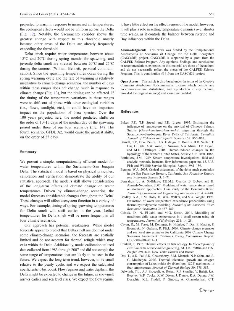
Fig. 13 Long-term shift in water temperatures on the SacramentoRiver at Rio Vista (station 15) under GFDL A2 forcing. Usingprojected temperatures, each day is grouped as it impacts the Deltasmelt: spring spawning (daily average temperatures from 15°C to 20°C in light gray), stress (daily average temperatures from 20°C to 25°Cin dark gray), and lethal (daily maximum temperatures >25°C inblack)

Fig. 12 Spatial variability in heating. Dot area is proportional to theaverage number of days per year exceeding 25°C (the Delta smelt’sthermal limit) at each location under GFDL A2 forcing. The blackdots represent the measured data; the dark gray dots are for 2010–2030; the light gray dots are for 2070–2090

Fig. 11 Projected yearly cycle of water temperatures at SacramentoRiver at Rio Vista (station 15) averaged from 2097 to 2099. The meanof the measured water temperatures at the same location from 1997 to1999 is included for comparison

Fig. 14 Projected shift in the median day of the spawning period dueto temperature on the Sacramento River at Rio Vista (station 15). Themedian day of the spawning period was calculated for each year undereach scenario. The medians were smoothed with a 10-year runningaverage

554 Estuaries and Coasts (2011) 34:544–556

projected to warm in response to increased air temperatures,the ecological effects would not be uniform across the Delta(Fig. 12). Notably, the Sacramento corridor shows thegreatest change with respect to this threshold mostlybecause other areas of the Delta are already frequentlyexceeding the threshold.

Delta smelt require water temperatures between about15°C and 20°C during spring months for spawning, andjuvenile delta smelt are stressed between 20°C and 25°Cduring the summer (William Bennett, personal communi-cation). Since the spawning temperatures occur during thespring warming cycle and the rate of warming is relativelyinsensitive to climate-change scenarios, the number of dayswithin these ranges does not change much in response toclimate change (Fig. 13), but the timing can be affected. Ifthe timing of the temperature variations in these rangeswere to drift out of phase with other ecological variables(i.e., flows, sunlight, etc.), it could have an importantimpact on the populations of these species. Over the100 years projected here, the model predicted shifts onthe order of 10–15 days of the median day of the spawningperiod under three of our four scenarios (Fig. 14). Thefourth scenario, GFDL A2, would cause the greatest shifts,on the order of 25 days.

Summary

We present a simple, computationally efficient model forwater temperatures within the Sacramento–San JoaquinDelta. The statistical model is based on physical principles;calibration and verification demonstrate the ability of ourstatistical approach. The model’s skill allows considerationof the long-term effects of climate change on watertemperatures. Driven by climate-change scenarios, themodel forecasts considerable changes throughout the Delta.These changes will affect ecosystem function in a variety ofways. For example, timing of spring spawning temperaturesfor Delta smelt will shift earlier in the year. Lethaltemperatures for Delta smelt will be more frequent in allfour climate scenarios.

Our approach has potential weaknesses. While modelforecasts appear to predict that Delta smelt are doomed undersome climate-change scenarios, the forecasts are spatiallylimited and do not account for thermal refugia which mayexist within the Delta. Additionally, model calibration utilizeddata collected from 1983 through 2007 and did not sample thesame range of temperatures that are likely to be seen in thefuture. We expect the long-term trend, however, to be smallrelative to the yearly cycle, and we expect the calculatedcoefficients to be robust. Flow regimes and water depths in theDelta might be expected to change in the future, as snowmeltarrives earlier and sea level rises. We expect the flow regime

to have little effect on the effectiveness of the model; however,it will play a role in setting temperature dynamics over shortertime scales, as it controls the balance between riverine andBay influences within the Delta.

Acknowledgments This work was funded by the ComputationalAssessments of Scenarios of Change for the Delta Ecosystem(CASCaDE) project. CASCaDE is supported by a grant from theCALFED Science Program. Any opinions, findings, and conclusionsor recommendations expressed in this material are those of the authorsand do not necessarily reflect the views of the CALFED ScienceProgram. This is contribution #19 from the CASCaDE project.

Open Access This article is distributed under the terms of the CreativeCommons Attribution Noncommercial License which permits anynoncommercial use, distribution, and reproduction in any medium,provided the original author(s) and source are credited.

References

Baker, P.F., T.P. Speed, and F.K. Ligon. 1995. Estimating theinfluence of temperature on the survival of Chinook SalmonSmolts (Oncorhynchus-tshawytscha) migrating through theSacramento–San-Joaquin River Delta of California. CanadianJournal of Fisheries and Aquatic Sciences 52: 855–863.

Barnett, T.P., D.W. Pierce, H.G. Hidalgo, C. Bonfils, B.D. Santer, T.Das, G. Bala, A.W. Wood, T. Nozawa, A.A. Mirin, D.R. Cayan,and M.D. Dettinger. 2008. Human-induced changes in thehydrology of the western United States. Science 319: 1080–1083.

Bartholow, J.M. 1989. Stream temperature investigations: field andanalytic methods. Instream flow information paper no. 13. U.S.Fish and Wildlife Service Biological Report, 89:1–139.

Bennett, W.A. 2005. Critical assessment of the delta smelt populationin the San Francisco Estuary, California. San Francisco Estuaryand Watershed Science 3: 1–71.

Benyahya, L., A. St-Hilaire, T.B.M.J. Ouarda, B. Bobee, and B.Ahmadi-Nedushan. 2007. Modeling of water temperatures basedon stochastic approaches: Case study of the Deschutes River.Journal of Environmental Engineering and Science 6: 437–448.

Bradley, A.A., F.M. Holly Jr., W.K. Walker, and S.A. Wright. 1998.Estimation of water temperature exceedance probabilities usingthermo-hydrodynamic modeling. Journal of the American WaterResources Association 3: 467–480.

Caissie, D., N. El-Jabi, and M.G. Satish. 2001. Modelling ofmaximum daily water temperatures in a small stream using airtemperatures. Journal of Hydrology 251: 14–28.

Cayan, D., M. Tyree, M. Dettinger, H. Hidalgo, T. Das, E. Maurer, P.Bromirski, N. Graham, R. Flick. 2009. Climate change scenariosand sea level rise estimates for California 2008 Climate ChangeScenarios Assessment: California Energy Commission Report:CEC-500-2009-014-D.

Coutant, C. 1976. Thermal effects on fish ecology. In Encyclopedia ofenvironmental science and engineering, ed. J.R. Pfafflin and E.N.Ziegler, 891–896. New York: Gordon and Breach.

Das, T., A.K. Pal, S.K. Chakraborty, S.M. Manush, N.P. Sahu, and S.C. Mukherjee. 2005. Thermal tolerance, growth and oxygenconsumption of Labeo rohita fry (Hamilton, 1822) acclimated tofour temperatures. Journal of Thermal Biology 30: 378–383.

Delworth, T.L., A.J. Broccoli, A. Rosati, R.J. Stouffer, V. Balaji, J.A.Beesley, W.F. Cooke, K.W. Dixon, J. Dunne, K.A. Dunne, J.W.Durachta, K.L. Findell, P. Ginoux, A. Gnanadesikan, C.T.

Estuaries and Coasts (2011) 34:544–556 555

Gordon, S.M. Griffies, R. Gudgel, M.J. Harrison, I.M. Held, R.S.Hemler, L.W. Horowitz, S.A. Klein, T.R. Knutson, P.J. Kushner,A.R. Langenhorst, H.C. Lee, S.J. Lin, J. Lu, S.L. Malyshev, P.C.D. Milly, V. Ramaswamy, J. Russell, M.D. Schwarzkopf, E.Shevliakova, J.J. Sirutis, M.J. Spelman, W.F. Stern, M. Winton,A.T. Wittenberg, B. Wyman, F. Zeng, and R. Zhang. 2006.GFDL’s CM2 global coupled climate models. Part I: Formulationand simulation characteristics. Journal of Climate 19: 643–674.

Fischer, H.B., E.J. List, R.C.Y. Koh, J. Imberger, and N.H. Brooks.1979. Mixing in inland and coastal waters. New York:Academic.

Garrick, M., C. Cunnane, and J.E. Nash. 1978. Criterion of efficiencyfor rainfall–runoff models. Journal of Hydrology 36: 375–381.

Hidalgo, H.G., M.D. Dettinger, D.R. Cayan. 2008. Downscaling withconstructed analogues—daily precipitation and temperature fieldsover the United States: California Energy Commission PIERFinal Project Report: CEC-500-2007-123.

Hotta, K., M. Tamura, T. Watanabe, Y. Nakamura, S. Adachi, and K.Yamauchi. 2001. Changes in spawning characteristics of Japa-nese whiting Sillago japonica under control of temperature.Fisheries Science 67: 1111–1118.

Johnson, T.B., and D.O. Evans. 1996. Temperature constraints onoverwinter survival of age-0 white perch. Transactions of theAmerican Fisheries Society 125: 466–471.

Kimmerer, W. 2004. Open water processes of the San FranciscoEstuary: From physical forcing to biological responses. SanFrancisco Estuary and Watershed Science 2.

Lemos, R.T., B. Sanso, and M.L. Huertos. 2007. Spatially varyingtemperature trends in a Central California estuary. Journal ofAgricultural Biological and Environmental Statistics 12: 379–396.

Loarie, S.R., B.E. Carter, K. Hayhoe, S. McMahon, R. Moe, C.A.Knight, and D.D. Ackerly. 2008. Climate change and the futureof California’s endemic flora. PLoS ONE 3: 1–10. doi:10.1371/journal.pone.0002502.

Lund, J., E. Hayak, W. Fleenor, R. Howitt, J. Mount, and P. Moyle.2007. Envisioning futures for the Sacramento–San JoaquinDelta. San Francisco: Public Policy Institute of California.

Marce, R., and J. Armengol. 2008. Modelling river water temperatureusing deterministic, empirical, and hybrid formulations in aMediterranean stream. Hydrological Processes 22: 3418–3430.

Meehl, G.A., C. Covey, T. Delworth, M. Latif, B. McAvaney, J.F.B.Mitchell, R.J. Stouffer, and K.E. Taylor. 2007. The WCRPCMIP3 multimodel dataset—a new era in climate changeresearch. Bulletin of the American Meteorological Society 88:1383–1394.

Miyakoda, K., and A. Rosati. 1984. The variation of sea-surfacetemperature in 1976 and 1977. 2. The simulation with mixed layermodels. Journal of Geophysical Research, Oceans 89: 6533–6542.

Mohseni, O., T.R. Erickson, and H.G. Stefan. 1999. Sensitivity ofstream temperatures in the United States to air temperaturesprojected under a global warming scenario. Water ResourcesResearch 35: 3723–3733.

Monismith, S.G., J.L. Hench, D.A. Fong, N.J. Nidzieko, W.E.Fleenor, L.P. Doyle, and S.G. Schladow. 2009. Thermalvariability in a tidal river. Estuaries and Coasts 32: 100–110.

Moyle, P.B., R.D. Baxter, T. Sommer, T.C. Foin, and S.A. Matern.2004. Biology and population dynamics of Sacramento Splittail(Pogonichthys macrolepidotus) in the San Francisco Estuary: Areview. San Francisco Estuary and Watershed Science 2: 1–47.

Myrick, C.A., and J.J. Cech. 2000. Swimming performances of fourCalifornia stream fishes: Temperature effects. EnvironmentalBiology of Fishes 58: 289–295.

Nash, J.E., and J.V. Sutcliffe. 1970. River flow forecasting throughconceptual models part I—a discussion of principles. Journal ofHydrology 10: 282–290.

Overland, J.E., and R.W. Preisendorfer. 1982. A significance test forprincipal components applied to a cyclone climatology. MonthlyWeather Review 110: 1–4.

Preisendorfer, R.W., and C.D. Mobley. 1988. Principal componentanalysis in meteorology and oceanography. New York: Elsevier.

Rubin, E.S., and C.I. Davidson. 2001. Introduction to engineering andthe environment. Boston: McGraw-Hill.

Scheller, R.M., V.M. Snarski, J.G. Eaton, and G.W. Oehlert. 1999. Ananalysis of the influence of annual thermal variables on theoccurrence of fifteen warmwater fishes. Transactions of theAmerican Fisheries Society 128: 257–264.

Sinokrot, B.A., and H.G. Stefan. 1993. Stream temperature dynamics—measurements and modeling.Water Resources Research 29: 2299–2312.

Stacey, M.T., J.R. Burau, and S.G. Monismith. 2001. Creation ofresidual flows in a partially stratified estuary. Journal ofGeophysical Research, Oceans 106: 17013–17037.

Swanson, C., T. Reid, P.S. Young, and J.J. Cech. 2000. Comparativeenvironmental tolerances of threatened delta smelt (Hypomesustranspacificus) and introduced wakasagi (H-nipponensis) in analtered California estuary. Oecologia 123: 384–390.

Uncles, R.J., and J.A. Stephens. 2001. The annual cycle oftemperature in a temperate estuary and associated heat fluxes tothe coastal zone. Journal of Sea Research 46: 143–159.

Vannote, R.L., and B.W. Sweeney. 1980. Geographic analysis ofthermal equilibria—a conceptual-model for evaluating the effectof natural and modified thermal regimes on aquatic insectcommunities. The American Naturalist 115: 667–695.

Vanrheenen, N.T., A.W. Wood, R.N. Palmer, and D.P. Lettenmaier.2004. Potential implications of PCM climate change scenarios forSacramento–San Joaquin river basin hydrology and waterresources. Climatic Change 62: 257–281.

Ward, J.V., and J.A. Stanford. 1982. Thermal responses in theevolutionary ecology of aquatic insects. Annual Review ofEntomology 27: 97–117.

Washington, W.M., J.W. Weatherly, G.A. Meehl, A.J. Semtner, T.W.Bettge, A.P. Craig, W.G. Strand, J. Arblaster, V.B. Wayland, R.James, and Y. Zhang. 2000. Parallel climate model (PCM)control and transient simulations. Climate Dynamics 16: 755–774.

556 Estuaries and Coasts (2011) 34:544–556