
A Regulator’s Perspective on Advanced Training Technologies:

forensic speech statistics - 2019-12-23a GSM Page 1 of 50
Statistical Models in Forensic Voice Comparison
Geoffrey Stewart Morrison
Forensic Speech Science Laboratory, Aston Institute for Forensic Linguistics, and Forensic Data Science Laboratory,
Computer Science Department, Aston University, Birmingham, United Kingdom
Forensic Evaluation Ltd, Birmingham, United Kingdom
https://orcid.org/0000-0001-8608-8207
Ewald Enzinger
Eduworks, Corvallis, Oregon, USA
Forensic Speech Science Laboratory, Aston Institute for Forensic Linguistics, and Forensic Data Science Laboratory,
Computer Science Department, Aston University, Birmingham, United Kingdom
https://orcid.org/0000-0003-2283-923X
Daniel Ramos
AUDIAS – Audio, Data Intelligence and Speech, Escuela Politécnica Superior, Universidad Autónoma de Madrid, Spain
https://orcid.org/0000-0001-5998-1489
Joaquín González-Rodríguez
AUDIAS – Audio, Data Intelligence and Speech, Escuela Politécnica Superior, Universidad Autónoma de Madrid, Spain
https://orcid.org/0000-0003-0910-2575
Alicia Lozano-Díez
AUDIAS – Audio, Data Intelligence and Speech, Escuela Politécnica Superior, Universidad Autónoma de Madrid, Spain
https://orcid.org/0000-0002-5918-8568
This is a preprint of:Morrison, G.S., Enzinger, E., Ramos, D., González-Rodríguez, J., Lozano-Díez, A. (2020). Statistical models in forensic voice comparison. In Banks, D.L., Kafadar, K., Kaye, D.H., Tackett, M. (Eds.) Handbook of Forensic Statistics. (Ch. 21). Boca Raton, FL: CRC.
forensic speech statistics - 2019-12-23a GSM Page 2 of 50
Abstract
This chapter describes a number of signal-processing and statistical-modeling techniques that
are commonly used to calculate likelihood ratios in human-supervised automatic approaches
to forensic voice comparison. Techniques described include mel-frequency cepstral
coefficients (MFCCs) feature extraction, Gaussian mixture model - universal background
model (GMM-UBM) systems, i-vector - probabilistic linear discriminant analysis (i-vector
PLDA) systems, deep neural network (DNN) based systems (including senone posterior i-
vectors, bottleneck features, and embeddings / x-vectors), mismatch compensation, and
score-to-likelihood-ratio conversion (aka calibration). Empirical validation of forensic-
voice-comparison systems is also covered. The aim of the chapter is to bridge the gap
between general introductions to forensic voice comparison and the highly technical
automatic-speaker-recognition literature from which the signal-processing and statistical-
modeling techniques are mostly drawn. Knowledge of the likelihood-ratio framework for the
evaluation of forensic evidence is assumed. It is hoped that the material presented here will
be of value to students of forensic voice comparison and to researchers interested in learning
about statistical modeling techniques that could potentially also be applied to data from other
branches of forensic science.
forensic speech statistics - 2019-12-23a GSM Page 3 of 50
1 Introduction
The purpose of forensic voice comparison (aka forensic speaker comparison, forensic speaker
recognition, and forensic speaker identification) is to assist a court of law to decide whether the voices
on two (or more) recordings were produced by the same speaker or by different speakers. For simplicity,
in the present chapter we will assume that there is one recording of a speaker of known identity (the
known-speaker recording) and one recording of a speaker whose identity is in question (the questioned-
speaker recording). Common scenarios include that the questioned-speaker recording is of a telephone
call made to a call center, is of an intercepted telephone call, or is made using a covert recording device,
and the known-speaker recording is of a police interview with a suspect or is of a telephone call made by
a person who is in custody. The known-speaker recording is often an existing recording in which the
identity of the speaker is not disputed, but sometimes a recording is made specifically for the purpose of
conducting a forensic-voice-comparison analysis (practice varies depending on jurisdiction, laboratory
policy, and the circumstances of the particular case).
There is usually a mismatch between the questioned- and known-speaker recordings in terms of speaker-
intrinsic conditions, or speaker-extrinsic conditions, or both. Speaker-intrinsic variability can be due to
multiple factors including differences in speaking style (e.g., casual versus formal and quiet versus loud),
emotion (e.g., calm, angry, happy, sad), tiredness or physical stress (e.g., being out of breath), and elapsed
time (the way a speaker speaks varies from minute to minute, hour to hour, day to day, etc. with larger
differences occurring over longer time periods, Kelly & Hansen, 2016). In addition, the words and
phrases that a speaker says vary from occasion to occasion. Speaker-extrinsic variability can be due to
multiple factors including background noise that can vary in loudness and type (e.g., office noise,
ventilation system noise, traffic noise, crowd noise – as well as noise being captured on the recording,
speaking in a noisy environment also causes speakers to change the way they speak), reverberation (e.g.,
echoes in rooms with hard walls and floors), distance of the speaker from the microphone, the quality of
the microphone and other components of the recording equipment, transmission of the recording through
different communication channels that distort and degrade the signal in different ways (e.g., landline
telephone, mobile telephone, Voice over Internet Protocol VoIP), and the format in which the recording
is saved (in order to reduce the file size formats such as MP3 distort and degrade the signal). Intrinsic
and extrinsic variability leads to mismatches between questioned- and known-speaker recordings within
cases, and leads to different conditions and different mismatches from case to case.
Historically and in present practice, a number of different approaches have been used to extract
information from voice recordings and a number of different frameworks have been used to draw
inferences from that information. In auditory and spectrographic approaches information is extracted
using subjective judgment, by listening to the recordings and by looking at graphical representations of
parts of the recordings respectively (spectrograms are time by frequency by intensity plots of the acoustic
signal). In conjunction with auditory and spectrographic approaches, inferences have almost invariably
been drawn on the basis of subjective judgment. In acoustic-phonetic and human-supervised automatic
forensic speech statistics - 2019-12-23a GSM Page 4 of 50
approaches information is extracted in the form of quantitative measurements of the acoustic properties
of the audio recordings. For the acoustic-phonetic approach, inferences can be drawn via statistical
models, although in practice it is more common for practitioners of this approach to draw inferences on
the basis of subjective judgment, e.g., by making a plot of the measured values from different recordings
and then looking at the plot. For the automatic approach, inferences are invariably drawn via the use of
statistical models. Even if inferences are drawn via statistical models, rather than directly reporting the
output of the statistical model many practitioners use the output of the statistical model as input to a
subjective judgment that also includes consideration of other information such as their subjective
judgment based on auditory and acoustic-phonetic approaches (for arguments against this practice see
Morrison and Stoel, 2014). It should be noted that even if the output of a quantitative-measurement and
statistical-model approach is directly reported, such an approach still requires subjective judgments in
decisions such as the choice of data used to train the statistical models. These subjective judgments are,
however, as far removed as possible from the forensic practitioner’s final conclusion, so of all the
approaches this one is most resistant to cognitive bias (for recent reviews of cognitive bias in the context
of forensic science see Found, 2015, Stoel et al., 2015, National Commission on Forensic Science, 2015,
Edmond et al., 2017).
As of December 2019, there are no published national or international standards specific to forensic voice
comparison. The England and Wales Forensic Science Regulator’s Codes of Practice and Conduct
(Forensic Science Regulator, 2017) and their appendices relating to specific branches of forensic science
are effectively national standards in that forensic laboratories in the UK can seek accreditation to the
Codes, usually in combination with accreditation to ISO 17025:2015 General Requirements for The
Competence of Testing and Calibration Laboratories. There is an appendix to the codes for Speech and
Audio Forensic Services (Forensic Science Regulator, 2016). The European Network of Forensic Science
Institutes (ENFSI) has published Methodological Guidelines for Best Practice in Forensic Semiautomatic
and Automatic Speaker Recognition (Drygajlo et al., 2015). The Speaker Recognition Subcommittee of
the Organization of Scientific Area Committees for Forensic Science (OSAC SR) has established a set
of principles for performing forensic voice comparison and is in the process of developing standards.
Both the ENFSI guidelines and the OSAC SR principles include use of the likelihood-ratio framework
for drawing inferences, and empirical validation of system performance under conditions reflecting those
of the cases to which they are applied. The Forensic Science Regulator’s codes also require methods to
be validated. In forensic voice comparison these are not new ideas: quantitative-measurement and
statistical-model based implementations of the likelihood-ratio framework date back to the 1990s, and
calls for forensic-voice-comparison systems to be empirically validated under conditions reflecting
casework conditions date back to the 1960s (for reviews see Morrison, 2009, and Morrison, 2014,
respectively). The ENFSI guidelines and the OSAC SR principles also include the use of transparent and
reproducible methods and procedures, and the use of procedures that reduce the potential for cognitive
bias. Morrison and Thompson (2017) and Morrison (2018a) have argued that transparent quantitative-

forensic speech statistics - 2019-12-23a GSM Page 5 of 50
measurement and statistical-model based implementation of the likelihood-ratio framework with
empirical validation under casework conditions would be the only practical way to comply with the
admissibility criteria set out in United States Federal Rules of Evidence 702 and the Daubert trilogy of
Supreme Court rulings (Daubert v. Merrell Dow Pharmaceuticals, 1993; General Electric v. Joiner,
1997; and Kumho Tire v. Carmichael, 1999), and those set out in England and Wales Criminal Practice
Directions (2015) section 19A.
In order to reduce the potential for cognitive bias, increase transparency and reproducibility, facilitate
validation under conditions reflecting casework conditions, and to draw inferences that are logically
correct, we believe that the most practical approach is the human-supervised automatic approach used
in conjunction with statistical-model based implementation of the likelihood-ratio framework with direct
reporting of the output of the statistical model. The performance of acoustic-phonetic approaches have
been found to be much poorer than the performance of automatic approaches (see Enzinger et al., 2012;
Zhang et al., 2013; Enzinger, 2014; Enzinger and Kasess, 2014; Jessen et al., 2014; Enzinger and
Morrison, 2017). Acoustic-phonetic approaches are also much more time-consuming and costly in skilled
human labor, which makes empirical validation practically difficult. In the present chapter, we therefore
discuss only the human-supervised automatic approach and statistical-model based implementation of
the likelihood-ratio framework. We assume the reader is familiar with the likelihood-ratio framework,
which has been described elsewhere in the present volume. Our aim is to provide an overview of a
number of signal-processing and statistical-modeling techniques that are commonly used to calculate
likelihood ratios in human-supervised automatic approaches to forensic voice comparison. We aim to
bridge the gap between general introductions to forensic voice comparison and the highly technical (and
often fragmented) automatic-speaker-recognition literature from which the signal-processing and
statistical-modeling techniques are mostly drawn. The automatic-speaker-recognition literature is often
fragmented because many influential papers are short conference-proceedings papers that do not provide
fully detailed descriptions of the techniques they apply.
For readers unfamiliar with forensic voice comparison, we recommend general introductions such as
Morrison and Thompson (2017), Morrison et al. (2018), and Morrison and Enzinger (2019). These
include discussions of the likelihood-ratio framework, empirical validation, and legal admissibility. In
the present chapter we go into greater technical detail regarding the calculation of likelihood ratios than
is provided in such general introductions, but still attempt to make the material relatively accessible to
an audience with a limited background in signal processing and statistical modeling. We have in mind
researchers from other branches of forensic science and students of forensic voice comparison. There are
alternatives to and multiple variants of many of the feature-extraction and statistical-modeling techniques
we describe below. We do not attempt to be comprehensive, and describe only some of the variants that
have commonly been used in forensic voice comparison. For overviews of automatic speaker recognition
in general see Kinnunen and Lee (2010), Hansen and Hasan (2015), Fernández Gallardo (2016) §2.4,
Ajili (2017) ch. 4 (and see Hansen and Bořil, 2018, for a review of intrinsic and extrinsic variability in
forensic speech statistics - 2019-12-23a GSM Page 6 of 50
the context of automatic speaker recognition). These publications cover some of the same topics as the
present chapter but are aimed at an audience with a background in signal processing.
The chapter is structured as follows:
• Section 2 describes extraction of features from voice recordings, in particular extraction of mel-
frequency cepstral coefficients (MFCCs).
• Section 3 describes mismatch compensation in the feature domain, in particular cepstral-mean
subtraction (CMS), cepstral-mean-and-variance normalization (CMVN), and feature warping.
• Section 4 describes the Gaussian mixture model - universal background model (GMM-UBM)
approach.
• Section 5 describes the identity-vector - probabilistic linear discriminant analysis (i-vector PLDA)
approach, including mismatch compensation in the i-vector domain using canonical linear
discriminant functions (CLDF). In the automatic-speaker-recognition literature, the latter is
known as linear discriminant analysis (LDA).
• Section 6 describes deep neural network (DNN) based approaches, in particular those using
senone posterior i-vectors, bottleneck features, and speaker embeddings (aka x-vectors).
• Section 7 describes score-to-likelihood-ratio conversion (aka calibration) using logistic
regression. This can be applied to the output of GMM-UBM, i-vector PLDA, or DNN-based
systems.
• Section 8 discusses empirical validation of forensic-voice-comparison systems.
GMM-UBM is an older approach, in use from about 2000. It has mostly been replaced by the i-vector
PLDA approach, in use from about 2010. We describe GMM-UBM because it is still used by some
forensic practitioners, it is somewhat more straightforward to describe than i-vector PLDA, and part of
the discussion of the GMM-UBM approach provides a foundation for understanding the i-vector PLDA
approach. Since about 2015 state-of-the-art systems in automatic-speaker-recognition research have been
based on DNNs, and commercial DNN-based forensic-voice-comparison systems were first released
around 2018. DNNs are generally used to create vectors (alternatives to i-vectors) that are then fed into
PLDA models.
Color versions of the figures in this chapter and other material related to the chapter are available at
http://handbook-of-forensic-statistics.forensic-voice-comparison.net/.
2 Feature extraction
In the context of forensic voice comparison, features are the acoustic measurements made on voice
forensic speech statistics - 2019-12-23a GSM Page 7 of 50
recordings. We describe the most commonly used features in automatic approaches to forensic voice
comparison, mel-frequency cepstral coefficients (MFCCs), and their derivatives, deltas and double deltas.
For reviews of feature extraction methods in automatic speaker recognition, see Chaudhary et al. (2017),
Dişken et al. (2017), and Tirumala et al. (2017).
2.1 Mel-frequency cepstral coefficients (MFCCs)
Mel-frequency cepstral coefficients (MFCCs; see Davis and Mermelstein, 1980) are spectral
measurements made at regular intervals, i.e., once every few milliseconds, during the sections of the
recording corresponding to the speech of the speaker of interest. The noun “cepstrum” and adjective
“cepstral” were coined by Bogert et al. (1963) via rearrangements of the letters in the words “spectrum”
and “spectral”. “Mel” refers to a frequency scaling that, unlike hertz, reflects human perception of
frequency (Stevens et al., 1937). MFCCs are standard in speech processing in general, not just in
automatic speaker recognition. In contrast to its use in automatic speech recognition, there is no
principled reason for using mel scaling for automatic speaker recognition. Other variants of cepstral
coefficients could be used, but MFCCs work well and are the most popular (Tirumala et al., 2017).
The steps for extracting MFCC measurements from voice recordings are described below, see also Figure
1 in which the numbers within black circles correspond to the numbered steps below.
1. The speech signal is multiplied by a bell-shaped window (e.g., a hamming window) with a
duration typically on the order of 20 ms. The shape of the window is designed to reduce the
impact of the window itself on the measurement of the spectrum (see Harris, 1978).
2. The power spectrum of the windowed signal is calculated using a discrete Fourier transform (DFT,
or for computational efficiency a fast Fourier transform, FFT). A complex waveform, such as a
windowed speech signal, can be constructed by adding together at each point in time the
instantaneous intensities of a series of simple sine waves (the idea that any arbitrary waveform
can be constructed using such a series is credited to Fourier, 1808). A Fourier analysis determines
the frequencies, intensities, and phases of the sine waves that would have to be added together to
make the observed complex waveform. The power spectrum consists of the frequencies and
intensities of the sine wave components. For automatic speaker recognition, information about
phase is usually discarded.
3. The power spectrum is multiplied by a filterbank. This is a series of triangular shaped filters, e.g.,
26 filters, that are equally spaced on the mel-frequency scale. Each filter has a 50% overlap with
each of its neighbors. Since forensic voice comparison often involves telephone recordings, the
frequency range covered by the filters may be restricted to the traditional landline telephone
bandpass (300 Hz – 3.4 kHz).
forensic speech statistics - 2019-12-23a GSM Page 8 of 50
4. The intensities of the filterbank outputs are scaled logarithmically. The fact that this is log
intensity will be relevant for feature domain mismatch compensation as described in Section 3
below.
5. A discrete cosine transform (DCT) is fitted to the output of the filterbank. A DCT is similar to a
Fourier transform but all components are cosines of the same phase (or the opposite phase if the
coefficient value is negative). The components are orthogonal: a constant, half a period of a cosine,
one period of a cosine, one and a half periods of a cosine, etc. The process of fitting a DCT
involves selecting values for the weights, or coefficients, on each component which result in the
best fit to the data. Using all the DCT coefficients, the values of the original data can be recovered.
Using only the first few DCT coefficients results in a smoothed version of the original data, i.e.,
a smoothed spectrum (aka a cepstrum). The higher order coefficients tend to capture statistical
noise.
6. The first few DCT coefficients (e.g., the 1st through 14th DCT coefficients) are used as a vector
of MFCCs. The 0th coefficient encodes the mean intensity of the signal and is usually discarded
since this can be affected by factors not related to who is speaking (e.g., the distance of the speaker
to the microphone or automatic gain control on the recording system).
The window is advanced in time, e.g., a 20-ms long window is advanced by 10 ms. Each range of time
covered by a window is called a frame, and there is usually a 50% overlap between adjacent frames.
Steps 1 through 6 are then repeated to produce another vector of MFCC values. The window is repeatedly
advanced until MFCC vectors have been extracted from all sections of the recording corresponding to
the speech of the speaker of interest. Since one MFCC vector is extracted every few milliseconds, a
relatively large number of feature vectors is extracted, e.g., 100 feature vectors per second if the frame
advance is 10 ms.
<Insert Figure 1 about here>
2.2 Deltas and double deltas
Deltas are derivatives of MFCCs and encode the local rate of change of MFCC values over time (see
Furui, 1986). Double deltas are the second derivatives of MFCCs and encode the local rate of change of
delta values over time. Vectors of deltas and double deltas are concatenated with the MFCC vectors to
produce longer feature vectors, e.g., if the original MFCC vector has 14 values, the MFCC + delta vector
will have 28, and the MFCC + delta + double delta vector will have 42.
Delta values are calculated separately for each MFCC dimension. In each dimension, a linear regression
is fitted to a contiguous set of MFCC values, e.g., the MFCC value at the frame in time where the delta
is being measured plus the MFCC values from the same dimension in the two preceding and the two
forensic speech statistics - 2019-12-23a GSM Page 9 of 50
following frames. Measurements are usually made over the ±2 or ±3 adjacent frames. The value of the
slope of the fitted linear regression is used as the delta value.
Double deltas are calculated in the same way as deltas, but based on the delta values rather than on the
MFCC values.
The statistical modeling steps of automatic-speaker-recognition systems usually discard information
regarding the original time sequence of the feature vectors, hence the deltas and double deltas encode the
only time-sequence information that is exploited. DNN embedding systems are an exception to this.
2.3 Voice-activity detection (VAD) and diarization
Either prior to or after extracting MFCCs, the speech of the speaker of interest should be separated from
periods of silence, transient noises, and the speech of other speakers. Either only the speech of the speaker
of interest should be measured, or only measurements corresponding to the speech of the speaker of
interest should be kept. This is done by either manually or automatically marking the beginning and end
of each utterance (stretch of speech) of interest. An automatic procedure may be followed by manual
checking and correction as needed.
The process of finding utterances is called voice-activity detection (VAD, aka speech-activity detection,
SAD). A simple automatic voice-activity detector (also abbreviated as VAD) may be based solely on
root-mean-square (RMS) amplitude, and thus simply find louder parts of the recording. Such simple
VADs may not, however, perform well under conditions that include background noise, as is common
in forensic voice comparison (see Mandasari et al. 2012). More sophisticated VADs employ algorithms
to distinguish speech from other sounds and noises (e.g., Sohn et al., 1999; Beritelli and Spadaccini, 2011;
Sadjadi and Hansen, 2013).
The process of attributing different utterances in the recording to different speakers is called diarization.
Automatic diarization is itself a form of automatic speaker recognition and may itself make use of
MFCCs.
3 Mismatch compensation in the feature domain
The acoustic properties of voice recordings can vary because they are produced by different speakers,
but also because of other factors such as differences in speaking styles (e.g., casual, formal, whispering,
shouting), differences in background noise and/or reverberation, differences in the distance of the speaker
to the microphone, different types of microphones, transmission through different communication
channels (e.g., landline telephone, mobile telephone, VoIP), and being saved in different formats (in
order to reduce the size of the files stored, formats such as MP3 use lossy compression which discards
some acoustic information and distorts remaining acoustic information). Mismatch compensation

forensic speech statistics - 2019-12-23a GSM Page 10 of 50
techniques seek to maximize between-speaker differences and minimize differences due to other factors.
Feature domain mismatch compensation techniques generally attempt to reduce differences due to
recording and transmission channels and differences due to acoustic noise.
We describe three commonly used feature domain mismatch compensation techniques: cepstral-mean
subtraction (CMS), cepstral-mean-and-variance normalization (CMVN), and feature warping.
3.1 Cepstral-mean subtraction (CMS) and Cepstral-mean-and-variance normalization
(CMVN)
Cepstral-mean subtraction (CMS; Furui, 1981) as a mismatch compensation technique is based on the
premise that the speech signal, which is changing rapidly over time, is convolved with a channel that is
invariant over time (it is linear time invariant, LTI). This is a good model for a traditional landline
telephone system, the effect of which is essentially to pass the speech signal through a bandpass filter.
Different microphones have different frequency responses. Some may be more sensitive to lower
frequency sounds, some to higher frequency sounds, etc. Microphones and other basic components of
recording systems can be treated as linear time invariant. Differences in the signal due to differences in
the distance from the speaker to the microphone can also be treated as linear time invariant effects, as
long as the distance does not change during the recording.
Convolution in the time domain is equivalent to multiplication in the frequency domain. Since MFCCs
are frequency domain representations they can be considered the result of multiplying the dynamic
speech signal and the invariant channel. But note that in generating MFCCs, intensity was logarithmically
scaled (Step 4 in Section 2.1 above). Multiplication on a linear scale is equivalent to addition on a
logarithmic scale, hence we should consider MFCCs the result of adding the speech signal and the
channel in the log frequency domain.
Assuming the channel is invariant over time, it can be estimated by taking the mean of the cepstral
coefficients over time. For the value in each dimension in each frame, the mean for that dimension is
subtracted. What remains are the dynamic aspects of the original MFCC features. Deltas and double
deltas are calculated on the raw MFCCs before CMS is applied to the MFCCs, and (although not
obviously theoretically motivated) CMS is then usually applied to the deltas and double deltas.
As well as removing the effect of the invariant channel, CMS also removes the speech signal’s mean. If
there is a substantial channel mismatch between the questioned- and known-speaker recordings,
removing the effect of the channel will tend to lead to better performance despite the loss of the speech-
signal mean information (but CMS will tend to lead to worse performance if there is in fact no channel
mismatch, Reynolds, 1994). For each recording, the mean of the feature values in each dimension will
be 0, hence statistical models applied to the post-CMS features are designed to exploit what remains:
non-normalities (in terms of skewness, kurtosis, and multimodalities), variance, and multidimensional
forensic speech statistics - 2019-12-23a GSM Page 11 of 50
correlations.
Although the theoretical motivation is less immediately obvious, cepstral-mean-and-variance
normalization (CMVN; Vikki and Laurila, 1998) is a statistically obvious extension to CMS in which,
as well as subtracting the mean, the variance of each MFCC dimension is scaled to 1.
CMS and CMVN can be applied globally, i.e., using the mean and variance of MFCC values from the
whole of the speech of the speaker of interest in a particular recording, or can be applied locally, i.e.,
using the mean and variance of the MFCC values from the speech of the speaker of interest within a
window that is a few seconds long. Such local application is discussed below in the context of feature
warping.
3.2 Feature warping
Rather than assuming that there is a channel effect that is invariant throughout the recording, feature
warping (Pelecanos and Sridharan, 2001) is based on the assumption that there may be a slowly changing
channel effect convolved with a rapidly changing speech signal. It also assumes that there may be slowly
changing additive noise. Since these are assumed to be slowly changing, their effect on the MFCC values
is assumed to be stable locally, i.e., over a period of a few seconds.
The implementation of feature warping is described below, see also Figure 2. Feature warping is applied
separately to each feature vector dimension. It is based on finding where the current feature value lies
relative to the empirical distribution of the values in, for example, the preceding 1.5 s and the following
1.5 s (±150 frames), and then warping that value to the corresponding value in a target distribution. The
target distribution is usually a Gaussian distribution with a mean of 0 and variance of 1.
1. Obtain the feature values from the 150 frames preceding the current frame, and the 150 frames
following the current frame.
2. Sort the 301 values (including the current value) in ascending order, and calculate each value’s
rank proportional to the total number of values. This can be represented graphically as a plot of
the empirical cumulative distribution of the feature values.
3. Find the value of the empirical cumulative distribution, yempirical, which corresponds to the current
feature value, xoriginal.
4. On the target cumulative probability distribution, locate the point ytarget = yempirical.
5. Read off the corresponding xwarped value from the target cumulative probability distribution.
<Insert Figure 2 about here>
Deltas and double deltas are calculated on the raw MFCCs before feature warping is applied to the

forensic speech statistics - 2019-12-23a GSM Page 12 of 50
MFCCs, and feature warping is then applied to the deltas and double deltas.
Figure 3 shows an example of the effect of applying feature warping to mismatched recording conditions.
The histograms in the leftmost column represent the distribution of the 1st order MFCC values extracted
from a studio-quality speech recording. The histograms in the next three columns show the distributions
of the 1st order MFCC values extracted after having applied various signal processing techniques to
simulate the different conditions of a questioned-speaker recording and a known-speaker recording from
a case (top and bottom rows respectively). Notice how the distributions change after each step and how
the distributions under the simulated questioned- and known-speaker conditions diverge from one
another. The histograms in the rightmost column show the distributions after feature warping is applied.
Notice how the distributions are now warped to approximate the same target distribution.
<Insert Figure 3 about here>
Making all univariate distributions the same may seem extreme, but the temporal ordering of vectors is
not altered and so correlations across dimensions are not lost. The correlations of interest are ultimately
due to time and frequency patterns in the acoustic signal resulting from the articulation of speech sounds.
Particular time and frequency patterns result from the articulation of particular speech sounds. Statistical
models applied to the warped features are designed to exploit these multidimensional correlations.
Empirically, feature warping can outperform CMS and CMVN (see for example: Pelecanos and
Sridharan, 2001; Silva and Medina, 2017).
4 GMM-UBM
This section describes the Gaussian mixture model - universal background model approach (GMM-UBM;
see Reynolds et al., 2000).
The GMM-UBM model is a specific-source model,1 i.e., it builds a model for the specific known-speaker
recording in the case, and thus answers the following two-part question:
What would be the probability of obtaining the feature vectors of the questioned-speaker
recording if the questioned speaker were the known speaker?
versus
What would be the probability of obtaining the feature vectors of the questioned-speaker
recording if the questioned speaker were not the known speaker, but some other speaker selected
at random from the relevant population?
Conceptually, the answer to the first part of the question provides the numerator for the likelihood ratio
1 For a discussion of the distinction between specific-source and common-source models, see Ommen and Saunders (2018).
forensic speech statistics - 2019-12-23a GSM Page 13 of 50
and the answer to the second part provides the denominator.
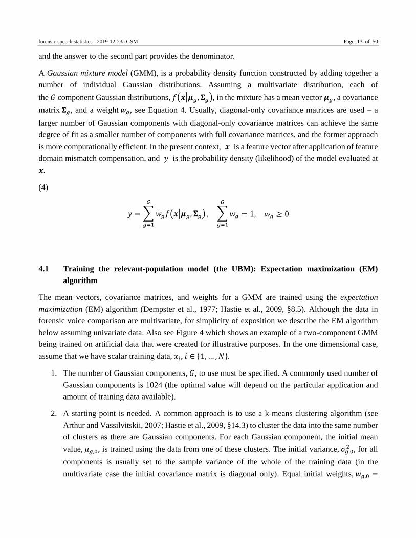
A Gaussian mixture model (GMM), is a probability density function constructed by adding together a
number of individual Gaussian distributions. Assuming a multivariate distribution, each of
the 𝐺 component Gaussian distributions, 𝑓(𝒙|𝝁𝑔, 𝚺𝑔), in the mixture has a mean vector 𝝁𝑔, a covariance
matrix 𝚺𝑔, and a weight 𝑤𝑔, see Equation 4. Usually, diagonal-only covariance matrices are used – a
larger number of Gaussian components with diagonal-only covariance matrices can achieve the same
degree of fit as a smaller number of components with full covariance matrices, and the former approach
is more computationally efficient. In the present context, 𝒙 is a feature vector after application of feature
domain mismatch compensation, and 𝑦 is the probability density (likelihood) of the model evaluated at
𝒙.
(4)
𝑦 = ∑ 𝑤𝑔𝑓(𝒙|𝝁𝑔, 𝚺𝑔)
𝐺
𝑔=1
, ∑ 𝑤𝑔
𝐺
𝑔=1
= 1, 𝑤𝑔 ≥ 0
4.1 Training the relevant-population model (the UBM): Expectation maximization (EM)
algorithm
The mean vectors, covariance matrices, and weights for a GMM are trained using the expectation
maximization (EM) algorithm (Dempster et al., 1977; Hastie et al., 2009, §8.5). Although the data in
forensic voice comparison are multivariate, for simplicity of exposition we describe the EM algorithm
below assuming univariate data. Also see Figure 4 which shows an example of a two-component GMM
being trained on artificial data that were created for illustrative purposes. In the one dimensional case,
assume that we have scalar training data, 𝑥𝑖, 𝑖 ∈ {1, … , 𝑁}.
1. The number of Gaussian components, 𝐺, to use must be specified. A commonly used number of
Gaussian components is 1024 (the optimal value will depend on the particular application and
amount of training data available).
2. A starting point is needed. A common approach is to use a k-means clustering algorithm (see
Arthur and Vassilvitskii, 2007; Hastie et al., 2009, §14.3) to cluster the data into the same number
of clusters as there are Gaussian components. For each Gaussian component, the initial mean
value, 𝜇𝑔,0, is trained using the data from one of these clusters. The initial variance, 𝜎𝑔,02 , for all
components is usually set to the sample variance of the whole of the training data (in the
multivariate case the initial covariance matrix is diagonal only). Equal initial weights, 𝑤𝑔,0 =
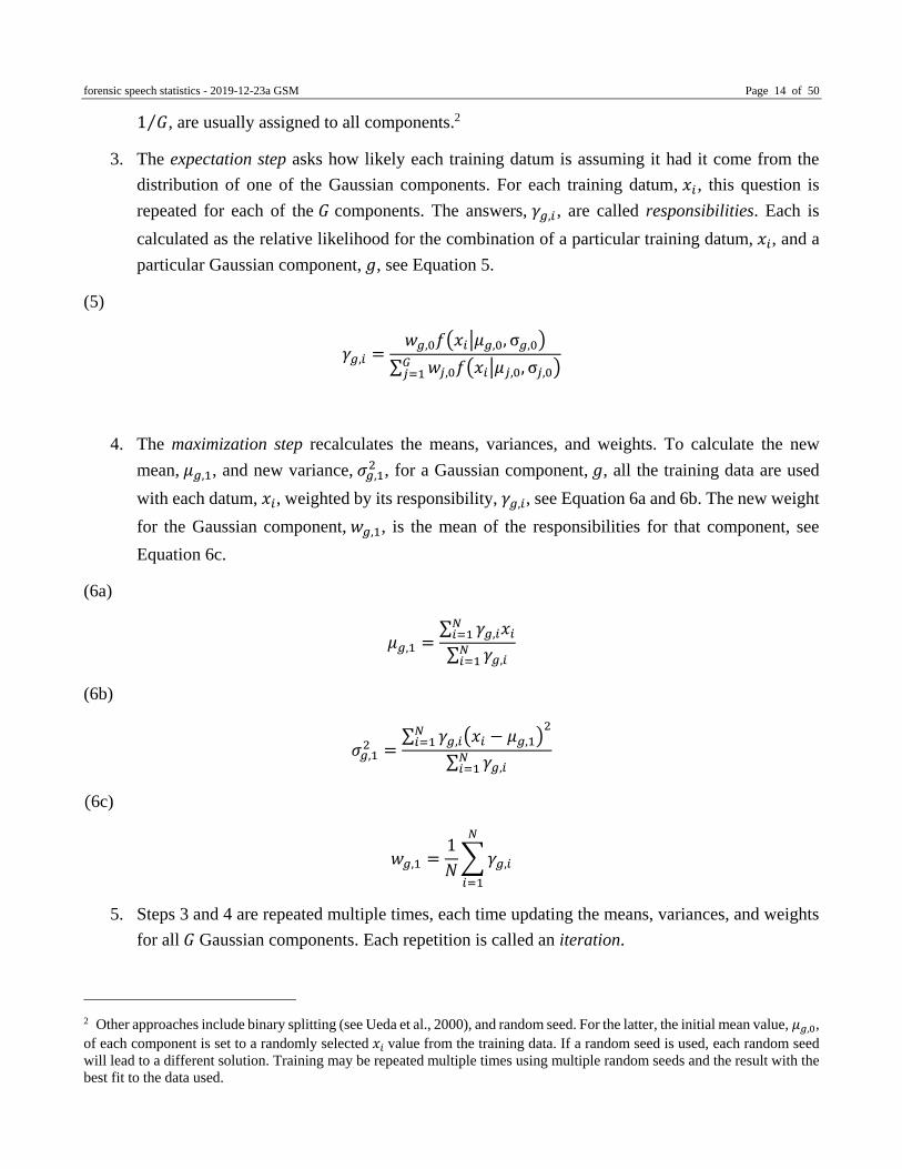
forensic speech statistics - 2019-12-23a GSM Page 14 of 50
1 𝐺⁄ , are usually assigned to all components.2
3. The expectation step asks how likely each training datum is assuming it had it come from the
distribution of one of the Gaussian components. For each training datum, 𝑥𝑖 , this question is
repeated for each of the 𝐺 components. The answers, 𝛾𝑔,𝑖 , are called responsibilities. Each is
calculated as the relative likelihood for the combination of a particular training datum, 𝑥𝑖, and a
particular Gaussian component, 𝑔, see Equation 5.
(5)
𝛾𝑔,𝑖 =𝑤𝑔,0𝑓(𝑥𝑖|𝜇𝑔,0, σ𝑔,0)
∑ 𝑤𝑗,0𝑓(𝑥𝑖|𝜇𝑗,0, σ𝑗,0)𝐺𝑗=1
4. The maximization step recalculates the means, variances, and weights. To calculate the new
mean, 𝜇𝑔,1, and new variance, 𝜎𝑔,12 , for a Gaussian component, 𝑔, all the training data are used
with each datum, 𝑥𝑖, weighted by its responsibility, 𝛾𝑔,𝑖, see Equation 6a and 6b. The new weight
for the Gaussian component, 𝑤𝑔,1, is the mean of the responsibilities for that component, see
Equation 6c.
(6a)
𝜇𝑔,1 =∑ 𝛾𝑔,𝑖𝑥𝑖
𝑁𝑖=1
∑ 𝛾𝑔,𝑖𝑁𝑖=1
(6b)
𝜎𝑔,12 =
∑ 𝛾𝑔,𝑖(𝑥𝑖 − 𝜇𝑔,1)2𝑁
𝑖=1
∑ 𝛾𝑔,𝑖𝑁𝑖=1
(6c)
𝑤𝑔,1 =1
𝑁∑ 𝛾𝑔,𝑖
𝑁
𝑖=1
5. Steps 3 and 4 are repeated multiple times, each time updating the means, variances, and weights
for all 𝐺 Gaussian components. Each repetition is called an iteration.
2 Other approaches include binary splitting (see Ueda et al., 2000), and random seed. For the latter, the initial mean value, 𝜇𝑔,0,
of each component is set to a randomly selected 𝑥𝑖 value from the training data. If a random seed is used, each random seed
will lead to a different solution. Training may be repeated multiple times using multiple random seeds and the result with the
best fit to the data used.

forensic speech statistics - 2019-12-23a GSM Page 15 of 50
6. The algorithm stops when it converges on a solution. Convergence occurs when, from one
iteration to the next, the change in the goodness of fit of the model to the training data becomes
smaller than a pre-specified threshold. Alternatively, the algorithm stops after a pre-specified
number of iterations.
<Insert Figure 4 about here>
The first step in using a GMM-UBM is to train a GMM using feature vectors extracted from recordings
of a sample of speakers representative of the relevant population for the case. Feature vectors from
recordings of all the speakers in the sample are pooled and used to train a GMM which is called a
universal background model (UBM). This is the model which will be used to calculate the denominator
of the likelihood ratio.
4.2 Training the known-speaker model: Maximum a posteriori (MAP) adaptation
The model for calculating the numerator of the likelihood ratio, a speaker model, is also a GMM, but
rather than training the model from scratch, the known-speaker GMM is adapted from the UBM
(Reynolds et al., 2000). One reason for this is that successful training of a GMM with a large number of
Gaussian components in a high dimensional space requires a large amount of training data. The UBM is
trained using data from a large number of speakers, but the known-speaker GMM has to be trained using
data from one speaker, and often only one relatively short recording of that speaker is available. The
procedure for adapting a single-speaker GMM from the UBM is a form of maximum a posteriori
adaptation (MAP). It is similar to the EM algorithm, but usually only one iteration of MAP adaptation
is applied, usually only the means are adapted, and the means are only partially adapted. A new mean is
the result of a weighted mixture of the original mean from the UBM, 𝜇𝑔,UBM, and what would be the new
mean if the standard EM algorithm were applied, 𝜇𝑔,EM (the latter is 𝜇𝑔,1 in Equation 6a above). The
new mean is calculated using Equation 7, in which 𝛼𝑔, the weight for mixing the EM and UBM means,
is known as the adaptation coefficient, and 𝜏 is known as the relevance factor.
(7)
𝜇𝑔,1 = 𝛼𝑔𝜇𝑔,EM + (1 − 𝛼𝑔)𝜇𝑔,UBM = 𝛼𝑔
∑ 𝛾𝑔,𝑖𝑥𝑖𝑁𝑖=1
∑ 𝛾𝑔,𝑖𝑁𝑖=1
+ (1 − 𝛼𝑔)𝜇𝑔,0
𝛼𝑔 =𝑁𝑤𝑔,1
𝑁𝑤𝑔,1 + 𝜏
If the new weight for a Gaussian component, 𝑤𝑔,1, is large, i.e., lots of adaptation training data are
associated with that Gaussian component, then 𝛼𝑔 is larger and the new mean depends more on the EM

forensic speech statistics - 2019-12-23a GSM Page 16 of 50
mean, whereas if 𝑤𝑔,1 is small, 𝛼𝑔 is smaller and the new mean depends more on the UBM mean.3 This
can therefore be thought of as a form of Bayesian adaptation with the UBM mean as the prior mean. The
more sample data associated with a Gaussian component the closer its posterior mean will be to the
sample mean. Increasing 𝜏 gives globally greater weight to the UBM means (the value for 𝜏 used in
Reynolds et al., 2000, was 16).
Figure 5 shows an example of a two-dimensional UBM and a MAP adapted known-speaker GMM.
<Insert Figure 5 about here>
4.3 Calculating a score
Assume that a multivariate UBM population model was trained on a sample of data from the relevant
population, and has mean vectors 𝝁𝑟𝑗, covariance matrices 𝚺𝑟𝑗
, and weights 𝑤𝑟𝑗, 𝑗 ∈ {1 … 𝐺}. Assume
that a multivariate GMM known-speaker model was trained on data from the known speaker, and has
mean vectors 𝝁𝑘𝑗, covariance matrices 𝚺𝑘𝑗
, and weights 𝑤𝑘𝑗, 𝑗 ∈ {1 … 𝐺}. Also, assume that the data
from the questioned-speaker recording consists of 𝑁𝑞 feature vectors: 𝒙𝑞𝑖, 𝑖 ∈ {1 … 𝑁𝑞}.
To calculate a likelihood ratio, Λ𝑞𝑖,𝑘, for a single feature vector from the questioned-speaker recording,
𝒙𝑞𝑖, the likelihood of the known-speaker model is evaluated given that feature vector, the likelihood of
the population model is evaluated given that feature vector, and the former is divided by the latter, see
Equation 8 and a graphical example in Figure 5.
(8)
Λ𝑞𝑖,𝑘 =∑ 𝑤𝑘𝑗
𝑓 (𝒙𝑞𝑖|𝝁𝑘𝑗
, 𝚺𝑘𝑗)𝐺
𝑗=1
∑ 𝑤𝑟𝑗𝑓 (𝒙𝑞𝑖
|𝝁𝑟𝑗, 𝚺𝑟𝑗
)𝐺𝑗=1
Note, however, that if a feature vector is extracted every 10 ms, then there will be 100 feature vectors for
every second of speech in the questioned-speaker recording. The total number of feature vectors, 𝑁𝑞,
from the questioned speaker recording may be in the thousands or tens of thousands. We do not want to
report a likelihood ratio at the first 10-ms mark, a likelihood ratio at the second 10-ms mark, etc. We
want to report a single value quantifying the strength of evidence associated with the whole of the
questioned-speaker speech. Our next step toward this is to calculate the mean of the per-feature-vector
log likelihood ratios, as in Equation 9.
3 If only the means are adapted, the “new” weights are only used for this calculation, and it is actually the old UBM weights
that are used for the speaker model.

forensic speech statistics - 2019-12-23a GSM Page 17 of 50
(9)
𝑆𝑞,𝑘 =1
𝑁𝑞∑ log(Λ𝑞𝑖,𝑘)
𝑁𝑞
𝑖=1
We will call the mean of the per-feature-vector log likelihood ratios, 𝑆𝑞,𝑘, a score. We will not call it a
likelihood ratio. Multiplying all the per-feature-vector likelihood ratios together, or adding all the per-
feature-vector log likelihood ratios together, is known as naïve Bayes fusion. It is naïve because it
assumes there is no correlation between the likelihood-ratio values being combined. So that score values
are not heavily dependent on the duration of the questioned-speaker recording, a score is calculated as
the mean of the per-feature-vector log likelihood-ratio values rather than as their sum, but this still ignores
correlation. In fact, the likelihood-ratio values come from a series of feature vectors taken from adjacent
frames of speech recording with 50% overlap between adjacent frames (see Section 2.1). Substantial
correlation between the frame-by-frame likelihood-ratio values is therefore expected. In addition, in
training the UBM and the GMM speaker models we have estimated a large number of parameter values,
e.g., 42 dimensions × (1024 means + 1024 variances) + 1024−1 weights = 87,039 parameter values.
Unless we had an extremely large amount of data, those estimates may be poor. Thus, we are not safe to
treat the value of 𝑆𝑞,𝑘 as an appropriate answer to the question posed by the same-speaker and different-
speaker hypotheses in the case. To fix this problem, we will implement an additional step: score-to-
likelihood-ratio conversion (aka calibration). This is the topic of Section 7 below – some readers may
wish to skip directly to Section 7 and return to Sections 5 and 6 later.
4.4 Remarks regarding UBM training data
The UBM is the model which represents the relevant population. The data used to train the UBM should
therefore be a sample that is representative of the relevant population in the case. In addition, the training
data should reflect the speaking style and recording conditions of the known-speaker recording. Any
mismatch between the questioned-speaker data and the data used to train the known-speaker model, the
model in the numerator of the likelihood ratio, will then be the same as the mismatch between the
questioned-speaker data and the data used to train the population model, the model in the denominator
of the likelihood ratio. Feature-level mismatch compensation techniques cannot be assumed to be 100%
effective, and a difference in the conditions of the data used to train the model in the numerator and the
model in the denominator would be expected to bias the calculated value of the score (see Morrison,
2018b).
5 i-vector PLDA

forensic speech statistics - 2019-12-23a GSM Page 18 of 50
5.1 i-vectors
An i-vector is a single vector representing the speaker information extracted from a single recording. The
“i” stands for “identity”. The lengths of i-vectors extracted from different recordings are the same
irrespective of the lengths of the recordings. i-vectors are described in: Kenny et al. (2005); Matrouf et
al. (2007); Dehak et al. (2011); Matějka et al. (2011); Bousquet et al. (2013).
Below we describe a set of procedures for calculating i-vectors that are one of the sets of procedures
tested in Bousquet et al. (2013). These are not the most commonly used procedures, but are
approximately equivalent to the more commonly used procedures and easier to explain and understand.
Further below, we give a brief overview of the more commonly used procedures, with additional details
provided in Appendix A.
To generate an i-vector from a speech recording, we begin by training a UBM on feature vectors extracted
from recordings of a large number of speakers under a variety of recording conditions. The standard
approach is to use a very large diverse set of speakers in a diverse range of recording conditions. Ideally,
the training data should include multiple recordings from each speaker, the multiple recordings including
different recording conditions. In the standard approach the training data for the UBM do not represent
the case-specific relevant population or the case-specific conditions.4
After training the UBM, the next step is to train a GMM for each recording in a set of recordings that are
representative of the relevant population for the case and that reflect the recording conditions of the
questioned- and known-speaker recordings in the case (when the amount of case-relevant data is small,
domain adaptation may be used, see García-Romero and McCree, 2014). The GMM for each recording
is trained using mean-only MAP adaptation from the UBM. Since each GMM is adapted from the same
UBM, the mean vectors in different GMMs have a parallel structure (they lie in the same vector space),
e.g., the first mean of the mean vector of the first component in the GMM for one recording is parallel to
the first mean of the mean vector of the first component in the GMM for another recording because they
were both adapted from the first mean of the mean vector of the first component in the UBM, mutatis
mutandis for every mean in the mean vector of every component. We take all the mean vectors from all
the components in the GMM, and concatenate them to form a supervector. For example, if we have 42
dimensional features, hence 42 dimensional mean vectors, we take the mean vector from the first
component, the mean vector from the second component, and concatenate them to form a vector that has
42 + 42 = 84 dimensions. We then concatenate the latter vector with the mean vector from the third
component to form a vector that has 84 + 42 = 126 dimensions. We continue until we have concatenated
the mean vectors from all the components. If there are 1024 components, the supervector has 43,008
4 Enzinger (2016) ch. 4, obtained favorable results when a relatively small amount of case-specific data were used for training
the UBM, i.e., data that represented the relevant population for the case and reflected the conditions of the questioned- and
known-speaker recordings in the case. One should be cautious, however, because training with small amounts of data may
give unstable results.

forensic speech statistics - 2019-12-23a GSM Page 19 of 50
dimensions. We generate one supervector for each recording of each speaker.
Next, we reduce the number of dimensions using principal component analysis (PCA). PCA finds new
dimensions which are linear combinations of the original dimensions such that the first PCA dimension
accounts for the largest amount of variance in the training data, the second PCA dimension accounts for
the largest remaining amount of variance in the training data after the first dimension is removed, the
third PCA dimension accounts for the largest remaining amount of variance in the training data after the
first and second dimensions are removed, etc. The number of dimensions is reduced by only using the
first few PCA dimensions. These dimensions capture most of the variance in the data. Figure 6 shows an
example of a reduction from two original dimensions to one PCA dimension. The PCA dimension is in
the direction of maximum variance in the original two-dimensional space. (The initial development of
PCA is credited to Pearson, 1901.)
<Insert Figure 6 about here>
The supervectors are reduced from tens of thousands of dimensions to a much smaller number of
dimensions, e.g., 400 dimensions. The reduced-dimension vectors are the i-vectors. The PCA dimensions
are in the directions of maximum variance in the original space, irrespective of whether the variance is
primarily due to speaker or condition (or other) differences, hence the result is sometimes called the total
variability space.
Conceptually, i-vectors are the result of a mapping from supervectors onto a linear subspace with a lower
number of dimensions. This is represented in Equation 10, in which 𝒔 is a recording-specific
supervector, 𝒎 is the supervector for the UBM, and 𝒗 is the i-vector for the specific recording (𝜺 is a
residual error term). 𝐓 is a low-rank matrix representing the linear subspace of the supervector space
on which the i-vectors lie. The 𝐓 matrix is designed such that the i-vectors have a few hundred
dimensions rather than the tens of thousands of dimensions of the supervectors.
(10)
𝒔 = 𝒎 + 𝐓𝒗 + 𝜺
The more commonly used procedures for extracting i-vectors do not use PCA for dimension reduction,
but instead a form of factor analysis. The 𝐓 matrix is trained using an iterative maximum likelihood
technique (the EM algorithm). Rather than first adapting a GMM from the UBM, then concatenating a
supervector, and then reducing its dimensions, a more direct procedure is used to map from feature
vectors to i-vectors. The first step is to calculate the Baum-Welch statistics for each recording. The 0th
order Baum-Welch statistics are based on the probability that a feature vector of a recording 𝑗 would
belong to component 𝑔 of the UBM (like the responsibilities in the EM algorithm). For each feature
vector, one value is calculated for each of the 𝐺 components, thus we have a matrix with 𝑁𝑗 columns
(as many columns as there are feature vectors in the recording) and 𝐺 rows of responsibilities. We then
sum over the columns to create a set of 𝐺 0th order statistics for recording 𝑗. The 1st order Baum-Welch

forensic speech statistics - 2019-12-23a GSM Page 20 of 50
statistics are based on the deviations of the feature vectors of a recording from the mean vector of each
component 𝑔 of the UBM, weighted by the probabilities that the feature vectors of the recording would
belong to component 𝑔 (the responsibilities of component 𝑔 for the feature vectors). Deviations are
calculated on a per-feature-dimension basis, hence for each of the 𝑁𝑗 feature vectors, 𝑀 values are
calculated for each of the 𝐺 components (where 𝑀 is the number of feature dimensions). We thus have
an 𝑁𝑗 by 𝑀 by 𝐺 matrix. We sum over the first of these dimensions to arrive at a set of 1st order
statistics for recording 𝑗, consisting of 𝐺 vectors each of length 𝑀. The 𝐓 matrix is trained using the
0th and 1st order Baum-Welch statistics from a set of training recordings, and an i-vector for a given
recording can then be directly calculated using the 𝐓 matrix and the 0th and 1st order Baum-Welch
statistics from that recording. We provide mathematical details in Appendix A. For greater detail, see the
references cited at the beginning of this section.
i-vectors are usually “whitened”, i.e., subjected to radial Gaussianization and length normalization, so
that they conform better to the assumptions of subsequent statistical modeling procedures (see García-
Romero and Espy-Wilson, 2009). After whitening it is only the direction of an i-vector away from the
origin of the i-vector space that is relevant (whitened i-vectors define points that lie on the hypersurface
of a hypersphere).
5.2 i-vector domain mismatch compensation (LDA)
A common i-vector domain mismatch compensation technique is known in the automatic-speaker-
recognition literature as linear discriminant analysis (LDA). In practice, linear discriminant analysis is
not actually performed (i.e., neither likelihoods, nor posterior probabilities, not classification results are
output), but canonical linear discriminant functions (CLDFs) are calculated and used to transform and
reduce the dimensionality of the i-vectors (see Klecka, 1980; Fisher, 1936, is credited with the initial
development of discriminant analysis and discriminant functions). In contrast to PCA which finds new
dimensions that maximize the total variance, LDA finds dimensions that maximize the ratio of between-
category variance versus within-category variance. CLDFs are trained, using i-vectors from training data
that include multiple recordings of each speaker, with different recordings in different conditions. Each
speaker is treated as a category, thus the CLDFs maximize the ratio of between-speaker variance to
within-speaker variance, much of the within-speaker variance being due to variability in speaking styles
and recording conditions. Only the first few CLDFs are used so as to primarily capture between-speaker
variance. The CLDFs are used to transform the i-vectors into a new smaller set of dimensions, e.g., 50
dimensions rather than 400.
Figure 7 shows an example of CLDF reduction from two dimensions to one dimension. The same data
are used for Figures 6 and 7 in order to illustrate the differences between the PCA and CLDF procedures.
CLDFs could be calculated for supervectors rather than i-vectors, but there can be problems with

forensic speech statistics - 2019-12-23a GSM Page 21 of 50
attempting to train CLDFs in such a high-dimensional space.
<Insert Figure 7 about here>
5.3 PLDA
An i-vector approach produces a single i-vector for each recording. Hence, unlike in the case of GMM-
UBM, there is a single vector for the known-speaker recording rather than a set of vectors that could be
used to train a known-speaker model. A different modeling approach is therefore used to calculate
likelihood ratios from i-vectors. In the automatic-speaker-recognition literature, this is known as
probabilistic linear discriminant analysis (PLDA). PLDA is described in: Prince and Elder (2007);
Kenny (2010); Brümmer and de Villiers (2010); Sizov et al. (2014).
PLDA is a common-source model,5 i.e., it does not build a model for the specific known-speaker
recording in the case, but instead answers the following two-part question:
What would be the probability of obtaining the feature vectors of the questioned-speaker
recording and the feature vectors of the known-speaker recording if the questioned speaker and
the known speaker were the same speaker, a speaker selected at random from the relevant
population?
versus
What would be the probability of obtaining the feature vectors of the questioned-speaker
recording and the feature vectors of the known-speaker recording if the questioned speaker and
the known speaker were different speakers, each selected at random from the relevant
population?6
Conceptually, the answer to the first part of the question provides the numerator for the likelihood ratio
and the answer to the second part provides the denominator.
Assume that we have a sample of 𝑁 speakers from the relevant population with multiple recordings of
each speaker, and that some recordings of each sample speaker are in the questioned-speaker condition
and others are in the known-speaker condition. We calculate an i-vector for each recording and apply i-
vector domain mismatch compensation. Imagine that we also have a known-speaker recording and a
questioned-speaker recording, and we calculate an i-vector for each of the two recording and apply i-
5 For a discussion of the distinction between specific-source and common-source models, see Ommen and Saunders (2018).
6 An objection may be raised that the known speaker was not selected at random, but on the basis of other evidence. The
forensic practitioner’s task, however, is to assess the strength of the particular evidence they have been asked to analyze –
they should not consider the other evidence in the case, considering all the evidence is the role of the trier of fact. For the
forensic practitioner’s task, it is therefore acceptable to make the statistical assumption that the known speaker was selected
at random from the relevant population.
forensic speech statistics - 2019-12-23a GSM Page 22 of 50
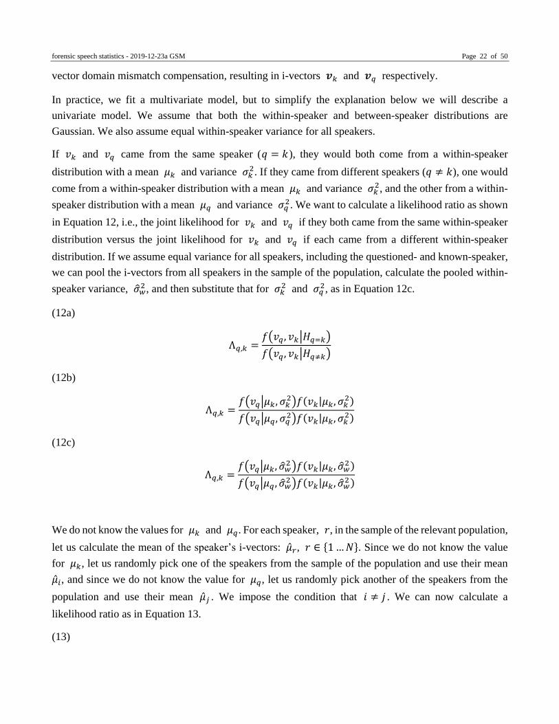
vector domain mismatch compensation, resulting in i-vectors 𝒗𝑘 and 𝒗𝑞 respectively.
In practice, we fit a multivariate model, but to simplify the explanation below we will describe a
univariate model. We assume that both the within-speaker and between-speaker distributions are
Gaussian. We also assume equal within-speaker variance for all speakers.
If 𝑣𝑘 and 𝑣𝑞 came from the same speaker (𝑞 = 𝑘), they would both come from a within-speaker
distribution with a mean 𝜇𝑘 and variance 𝜎𝑘2. If they came from different speakers (𝑞 ≠ 𝑘), one would
come from a within-speaker distribution with a mean 𝜇𝑘 and variance 𝜎𝑘2, and the other from a within-
speaker distribution with a mean 𝜇𝑞 and variance 𝜎𝑞2. We want to calculate a likelihood ratio as shown
in Equation 12, i.e., the joint likelihood for 𝑣𝑘 and 𝑣𝑞 if they both came from the same within-speaker
distribution versus the joint likelihood for 𝑣𝑘 and 𝑣𝑞 if each came from a different within-speaker
distribution. If we assume equal variance for all speakers, including the questioned- and known-speaker,
we can pool the i-vectors from all speakers in the sample of the population, calculate the pooled within-
speaker variance, �̂�𝑤2 , and then substitute that for 𝜎𝑘
2 and 𝜎𝑞2, as in Equation 12c.
(12a)
Λ𝑞,𝑘 =𝑓(𝑣𝑞 , 𝑣𝑘|𝐻𝑞=𝑘)
𝑓(𝑣𝑞 , 𝑣𝑘|𝐻𝑞≠𝑘)
(12b)
Λ𝑞,𝑘 =𝑓(𝑣𝑞|𝜇𝑘, 𝜎𝑘
2)𝑓(𝑣𝑘|𝜇𝑘, 𝜎𝑘2)
𝑓(𝑣𝑞|𝜇𝑞, 𝜎𝑞2)𝑓(𝑣𝑘|𝜇𝑘, 𝜎𝑘
2)
(12c)
Λ𝑞,𝑘 =𝑓(𝑣𝑞|𝜇𝑘, �̂�𝑤
2 )𝑓(𝑣𝑘|𝜇𝑘, �̂�𝑤2 )
𝑓(𝑣𝑞|𝜇𝑞, �̂�𝑤2 )𝑓(𝑣𝑘|𝜇𝑘, �̂�𝑤
2 )
We do not know the values for 𝜇𝑘 and 𝜇𝑞. For each speaker, 𝑟, in the sample of the relevant population,
let us calculate the mean of the speaker’s i-vectors: �̂�𝑟, 𝑟 ∈ {1 … 𝑁}. Since we do not know the value
for 𝜇𝑘, let us randomly pick one of the speakers from the sample of the population and use their mean
�̂�𝑖, and since we do not know the value for 𝜇𝑞, let us randomly pick another of the speakers from the
population and use their mean �̂�𝑗 . We impose the condition that 𝑖 ≠ 𝑗 . We can now calculate a
likelihood ratio as in Equation 13.
(13)
forensic speech statistics - 2019-12-23a GSM Page 23 of 50
Λ𝑞,𝑘,𝑖,𝑗 =𝑓(𝑣𝑞|�̂�𝑖 , �̂�𝑤
2 )𝑓(𝑣𝑘|�̂�𝑖 , �̂�𝑤2 )
𝑓(𝑣𝑞|�̂�𝑗 , �̂�𝑤2 )𝑓(𝑣𝑘|�̂�𝑖 , �̂�𝑤
2 )
If we pick two more speakers at random, we will calculate a different value for the likelihood ratio. Let
us imagine that we pick lots of random pairs of speakers and consider the average likelihood-ratio value.
If 𝑣𝑘 and 𝑣𝑞 are far apart, then the numerator of the likelihood ratio will always be relatively small
because 𝜇𝑖 cannot be close to both 𝑣𝑘 and 𝑣𝑞. The denominator of the likelihood ratio will sometimes
be relatively high because it is possible for 𝜇𝑖 to be close to 𝑣𝑘 and 𝜇𝑗 to be close to 𝑣𝑞. On average,
the denominator will be larger than the numerator and the average value of the likelihood ratio will
therefore be low.
If 𝑣𝑘 and 𝑣𝑞 are close to each other and atypical with respect to the population, i.e., both out on the
same tail of the distribution, then the value of the numerator of the likelihood ratio will usually be small
because the probability of 𝜇𝑖 being close to 𝑣𝑘 and 𝑣𝑞 is small, but when 𝜇𝑖 is close to 𝑣𝑘 and 𝑣𝑞
the value of the numerator will be large. On average the value of the denominator will be even lower
because the probability of both 𝜇𝑖 and 𝜇𝑗 being out on the same tail of the distribution and therefore
one being close to 𝑣𝑘 and the other being close to 𝑣𝑞 will be lower than the probability of only 𝜇𝑖
being out on that tail of the distribution. On average, the numerator will be larger than the denominator
and the average value of the likelihood ratio will therefore be high.
If 𝑣𝑘 and 𝑣𝑞 are close to each other but typical with respect to the population, i.e., both in the middle
of the distribution, then the value of the numerator of the likelihood ratio will usually be large because
the probability of 𝜇𝑖 being in the middle of the distribution and therefore being close to 𝑣𝑘 and 𝑣𝑞
will be large, but the value of the denominator will also usually be large because the probability of both
𝜇𝑖 and 𝜇𝑗 being in the middle of the distribution and therefore one being close to 𝑣𝑘 and the other
being close to 𝑣𝑞 will also be large. On average, the values of numerator and denominator will be about
the same and the average value of the likelihood ratio will therefore be close to 1.
In general, the average calculated value of the likelihood ratio will reflect how similar 𝑣𝑘 and 𝑣𝑞 are
to each other, and how typical they are with respect to the sample of the population.
Rather than selecting pairs of speakers at random, we could systematically go through all possible
combinations of speakers in our sample of the population and calculate the mean likelihood ratio, as in
Equation 14 (the sum in parenthesis in the denominator is from 1 to 𝑁−1 since 𝑗= 𝑖 is skipped).
(14)
forensic speech statistics - 2019-12-23a GSM Page 24 of 50
Λ𝑞,𝑘 =
1𝑁
∑ (𝑓(𝑣𝑞|�̂�𝑖 , �̂�𝑤2 )𝑓(𝑣𝑘|�̂�𝑖 , �̂�𝑤
2 ))𝑁𝑖=1
1𝑁
∑ (𝑓(𝑣𝑘|�̂�𝑖 , �̂�𝑤2 ) 1
𝑁−1∑ 𝑓(𝑣𝑞|�̂�𝑗 , �̂�𝑤
2 )𝑁−1𝑗=1 , 𝑗 ≠ 𝑖)𝑁
𝑖=1
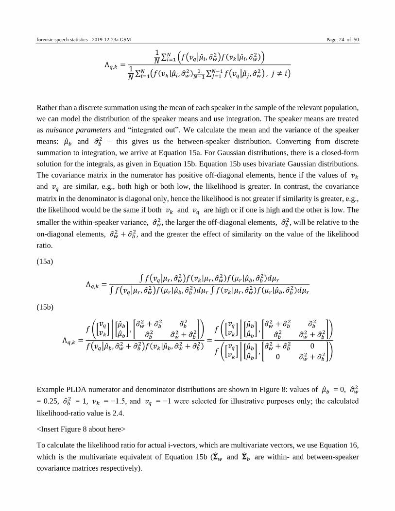
Rather than a discrete summation using the mean of each speaker in the sample of the relevant population,
we can model the distribution of the speaker means and use integration. The speaker means are treated
as nuisance parameters and “integrated out”. We calculate the mean and the variance of the speaker
means: �̂�𝑏 and �̂�𝑏2 – this gives us the between-speaker distribution. Converting from discrete
summation to integration, we arrive at Equation 15a. For Gaussian distributions, there is a closed-form
solution for the integrals, as given in Equation 15b. Equation 15b uses bivariate Gaussian distributions.
The covariance matrix in the numerator has positive off-diagonal elements, hence if the values of 𝑣𝑘
and 𝑣𝑞 are similar, e.g., both high or both low, the likelihood is greater. In contrast, the covariance
matrix in the denominator is diagonal only, hence the likelihood is not greater if similarity is greater, e.g.,
the likelihood would be the same if both 𝑣𝑘 and 𝑣𝑞 are high or if one is high and the other is low. The
smaller the within-speaker variance, �̂�𝑤2 , the larger the off-diagonal elements, �̂�𝑏
2, will be relative to the
on-diagonal elements, �̂�𝑤2 + �̂�𝑏
2, and the greater the effect of similarity on the value of the likelihood
ratio.
(15a)
Λ𝑞,𝑘 =∫ 𝑓(𝑣𝑞|𝜇𝑟 , �̂�𝑤
2 )𝑓(𝑣𝑘|𝜇𝑟 , �̂�𝑤2 )𝑓(𝜇𝑟|�̂�𝑏, �̂�𝑏
2)𝑑𝜇𝑟
∫ 𝑓(𝑣𝑞|𝜇𝑟 , �̂�𝑤2 )𝑓(𝜇𝑟|�̂�𝑏, �̂�𝑏
2)𝑑𝜇𝑟 ∫ 𝑓(𝑣𝑘|𝜇𝑟 , �̂�𝑤2 )𝑓(𝜇𝑟|�̂�𝑏, �̂�𝑏
2)𝑑𝜇𝑟
(15b)
Λ𝑞,𝑘 =
𝑓 ([𝑣𝑞
𝑣𝑘] | [
�̂�𝑏
�̂�𝑏] , [
�̂�𝑤2 + �̂�𝑏
2 �̂�𝑏2
�̂�𝑏2 �̂�𝑤
2 + �̂�𝑏2])
𝑓(𝑣𝑞|�̂�𝑏, �̂�𝑤2 + �̂�𝑏
2)𝑓(𝑣𝑘|�̂�𝑏, �̂�𝑤2 + �̂�𝑏
2)=
𝑓 ([𝑣𝑞
𝑣𝑘] | [
�̂�𝑏
�̂�𝑏] , [
�̂�𝑤2 + �̂�𝑏
2 �̂�𝑏2
�̂�𝑏2 �̂�𝑤
2 + �̂�𝑏2])
𝑓 ([𝑣𝑞
𝑣𝑘] | [
�̂�𝑏
�̂�𝑏] , [
�̂�𝑤2 + �̂�𝑏
2 0
0 �̂�𝑤2 + �̂�𝑏
2])
Example PLDA numerator and denominator distributions are shown in Figure 8: values of �̂�𝑏 = 0, �̂�𝑤2
= 0.25, �̂�𝑏2 = 1, 𝑣𝑘 = −1.5, and 𝑣𝑞 = −1 were selected for illustrative purposes only; the calculated
likelihood-ratio value is 2.4.
<Insert Figure 8 about here>
To calculate the likelihood ratio for actual i-vectors, which are multivariate vectors, we use Equation 16,
which is the multivariate equivalent of Equation 15b (�̂�𝑤 and �̂�𝑏 are within- and between-speaker
covariance matrices respectively).

forensic speech statistics - 2019-12-23a GSM Page 25 of 50
(16)
Λ𝑞,𝑘 =
𝑓 ([𝒗𝑞
𝒗𝑘] | [
�̂�𝑏
�̂�𝑏] , [
�̂�𝑤 + �̂�𝑏 �̂�𝑏
�̂�𝑏 �̂�𝑤 + �̂�𝑏
])
𝑓(𝒗𝑞|�̂�𝑏, �̂�𝑤 + �̂�𝑏)𝑓(𝒗𝑘|�̂�𝑏, �̂�𝑤 + �̂�𝑏)
In practice, the output of PLDA is treated as a score and subjected to score-to-likelihood-ratio conversion,
see Section 7.
What we have described above is known as the two-covariance version of PLDA. There are at least two
other versions of PLDA (that Sizov et al., 2014, label standard and simplified). The latter are more
complex than the two-covariance version in that they include dimension reduction to work in speaker-
variability and session-variability subspaces. Since the latter include subspace modeling, they are not
usually preceded by CLDF transformation, whereas since the two-covariance version does not include
subspace modeling it should be preceded by CLDF transformation. For further details of the two-
covariance version of PLDA and for details of the standard and simplified versions of PLDA, see the
references cited at the beginning of this section. For a comparison of the three, see Sizov et al. (2014).
6 DNN-based systems
Artificial neural networks are machine learning models that consist of nodes (neurons) that are organized
in layers, and connections between the nodes (synapses). An example of the architecture of an artificial
neural network is shown in Figure 9. This is an example of a standard feedforward fully-connected
architecture, i.e., all units in a given layer are connected to all the units in the preceding layer and all the
units in the following layer. The example has an input layer, two hidden layers, and an output layer. A
hidden layer is any layer other than the input or output layer. The number of hidden layers is a design
choice (this example happens to have two hidden layers). An artificial neural network with more than
one hidden layer is known as a deep neural network (DNN). A value is presented at each input node, e.g.,
the set of input nodes accepts a feature vector, 𝒙. Each input node then has an activation level, ℎ0,𝑛𝑎,
corresponding to an 𝑥 value. Each input node is connected to each node in the first hidden layer via
connections each of which is given a weight, 𝑤𝑙𝑗−1,𝑛𝑎,𝑙𝑗,𝑛𝑏, where 𝑙𝑗−1 and 𝑙𝑗 index the layers (in this
case the input layer, 𝑙𝑗−1 = 0, and the first hidden layer, 𝑙𝑗 = 1), and 𝑛𝑎 and 𝑛𝑏 index the particular
nodes that are connected. Each node in the first hidden layer then has an activation level, ℎ𝑙𝑗,𝑛𝑏, that is
a function, 𝜑, of the weighted sum of the values presented to the input layer, see Equation 17 (𝑏𝑙𝑗,𝑛𝑏 is
a node-specific bias term). A non-linear function, e.g., a sigmoidal function, is usually used.
(17)

forensic speech statistics - 2019-12-23a GSM Page 26 of 50
ℎ𝑙𝑗,𝑛𝑏= 𝜑 (𝑏𝑙𝑗,𝑛𝑏
+ ∑ 𝑤𝑙𝑗−1,𝑛𝑎,𝑙𝑗,𝑛𝑏ℎ𝑙𝑗−1,𝑛𝑎
𝑁𝑎
𝑛𝑎=1
)
The activation levels of nodes in higher layers are in turn based on weighted sums of the activation levels
of the nodes in the immediately preceding layer.
<Insert Figure 9 about here>
Usually, the task of the network is to predict the category that the input belongs to, and each node in the
output layer represents a category. For example, for an optical character recognition system, the input
could be an image of a character (i.e., a letter of the alphabet, a number, or a punctuation mark), each
output node would represent a particular character, and the relative level of activation of an output node
would represent the strength of the model’s prediction that the input image is of the character
corresponding to that output node. All else being equal, in order to classify the image, one would select
the character corresponding to the output node with the highest level of activation. The activations of the
output nodes can be scaled to represent posterior probabilities.
Training an artificial neural network is the process of setting the connection weights (and node-specific
biases) so as to optimize the network’s performance on the classification task. A standard supervised
training algorithm is backpropagation. This is an iterative process similar to the EM algorithm. Starting
from an initial state (e.g., a random seeding of the weights), it involves presenting inputs for which the
categories are known, comparing the activation levels of the output nodes with the desired activation
levels given the known category of the input, and adjusting the weights so as to reduce the error, i.e., to
lead to higher relative activation of the output node corresponding to the known category of the input.
For more detailed introductions to artificial neural networks, including network training, see Duda et al.
(2000) ch. 6, and Hastie et al. (2009) ch. 11.
Below, we briefly describe three DNN approaches: (1) DNN senone posterior i-vector systems, (2)
Bottleneck-feature based systems, and (3) DNN speaker embedding (x-vector) systems. All three were
common in state-of-the-art automatic-speaker-recognition systems when we began writing the present
chapter in 2017. By 2019 the x-vector approach had emerged as the clear winner.
6.1 DNN senone posterior i-vector systems
A senone posterior i-vector system can be considered a variant of an i-vector PLDA system, but using a
DNN to train the UBM rather than using the EM algorithm (see García-Romero et al., 2014; Kenny et
al., 2014; Lei et al., 2014). In contrast to standard i-vectors, senone posterior i-vectors are designed to
explicitly capture information about how speakers pronounce speech sounds.
forensic speech statistics - 2019-12-23a GSM Page 27 of 50
The input to the DNN consists of a series of feature vectors (e.g., MFCC + delta + double delta). The
DNN is trained to classify the input into sequences of speech sounds, e.g., triphones. For simplicity, we
present an example based on orthography rather than speech sounds: The word “forensic” contains the
trigraphs “for”, “ore”, “ren”, “ens”, “nsi”, and “sic”. In general, the sequences of speech sounds are called
senones. (Although there has been a shift and broadening of meaning to its current use in automatic
speaker recognition, the term “senone” was originally coined in Hwang and Huang, 1992, to mean a
subphonetic unit.)
Standard supervised training techniques are used to train the DNN to classify a large number of different
senones (e.g., between 5000 and 10,000). A “true” category label for the senone corresponding to each
feature vector is typically computed using an automatic-speech-recognition system. The DNN is trained
using a large number of recordings for a large number of speakers in diverse recording conditions. The
activation of each output node of the DNN is scaled to represent the posterior probability for the senone
it was trained on.
The UBM consist of a GMM in which each component Gaussian corresponds to a DNN output node.
Feature vectors from a new set of multiple recordings of multiple speakers are presented to the DNN.
The activation of each DNN output node, 𝑔, is obtained for each feature vector, 𝒙𝑖, and is used as the
responsibility, 𝛾𝑔,𝑖, in Equation 6 (the version of Equation 6 given in Section 4.1 was for univariate data,
the corresponding multivariate version is actually used). The 𝒙𝑖 and 𝛾𝑔,𝑖 provide all the information
necessary to train the UBM in a single iteration.
6.2 Bottleneck-feature based systems
In a bottleneck-feature based system (see Yaman et al., 2012; García-Romero and McCree, 2015;
Lozano-Díez et al., 2016; Matějka et al., 2016) a DNN is trained in the same way as in the senone
posterior i-vector system but one layer in the DNN, the bottleneck layer, has a substantially smaller
number of nodes than the other hidden layers, e.g., 60–80 nodes in the bottleneck layer compared to
1000–1500 nodes in other layers. The bottleneck layer is designed to capture information about the
phonetic content of voice recordings. The small number of nodes provides a compact representation of
this information. The bottleneck layer may be between other hidden layers, or may be immediately before
the output layer.
For each input feature vector (e.g., MFCC + delta + double delta), the activations of the nodes in the
bottleneck layer are used as a new feature vector, a bottleneck-feature vector. The bottleneck-feature
vectors are usually concatenated with the original MFCC + delta + double delta feature vectors and the
concatenated feature vectors then used as input to a standard UBM-based i-vector PLDA system (note
that the activations of the DNN’s output layer are not used).

forensic speech statistics - 2019-12-23a GSM Page 28 of 50
6.3 DNN speaker embedding systems (x-vector systems)
A DNN speaker embedding system is described in Snyder et al. (2017), and specific values given below
are those of that system (other variants are described in: Peddinti, Chen, et al., 2015; Peddinti, Povey,
and Khudanpur, 2015; Snyder et al., 2018). In this context, embeddings are fixed-length vectors that are
used instead of i-vectors as input to PLDA. These embeddings are also known as x-vectors. In contrast
to senone posterior i-vector systems and bottleneck-feature systems that are trained to classify senones,
a DNN embedding system is trained to classify speakers.
Rather than the input layer of a DNN speaker embedding system accepting a single feature vector, it is
organized to accept a two-dimensional matrix in which one dimension is the elements of the MFCC
vectors (that represent the frequency components of the signal at the time corresponding to each vector),
and the other dimension is time. Time is discretized according to the frame shifts used when extracting
the series of MFCC vectors from the voice recording. Deltas and double deltas are not included in the
input feature vectors, instead each node in the input layer is connected to the MFCC vectors from 5
contiguous frames, i.e., the MFCC vectors corresponding to the frames at times t–2, t–1, t, t+1, t+2.
Nodes in the first hidden layer are connected to nodes at times t–2, t, t+2 of the input layer, and nodes
the second hidden layer are connected to nodes at times t–3, t, t+3 of the first hidden layer, see Figure
10. The input layer ultimately spans frames t–7 to t+7.7 The second hidden layer is followed by two
more hidden layers that are unidimensional – their nodes are only connected to nodes at time t of the
preceding layer, hence the time dimension has been collapsed. All the layers described so far are called
frame-level layers. Layers that receive inputs from multiple times are said to splice those inputs together.
<Insert Figure 10 about here>
The next layer in the DNN is called a statistics-pooling layer. The whole sequence of MFCC vectors
from the speech of the speaker of interest in a recording is presented to the system, the input layer sees
15 frames at a time (frames t–7 through t+7) and t is advanced one frame at a time through the entire
sequence of MFCC vectors. For each node in the immediately preceding layer, the statistics-pooling layer
has two nodes, one calculates the mean of the activation of the preceding layer’s node over all t, and the
other calculates the standard deviation of the activation of the preceding layer’s node over all t. The
statistics-pooling layer provides a fixed-length vector irrespective of the length of the recording.
The values of the statistics-pooling layer are used as an input vector to a set of three more layers,
including the output layer. These are called segment-level layers.8 The second of these layers has fewer
7 The weights for the connections from the input layer to the nodes in the first hidden layer are not independent of each other.
The weights on different connections entering a first-layer node generally differ from each other, but the same set of weights
are used for the set of connections entering each and every first-layer node.
8 In the automatic-speaker-recognition literature, the term “segment” refers to all the speech of the speaker of interest in the
whole recording. It is the latter meaning which is intended, as opposed to the meaning of “segment” in phonetics, which is an
individual speech sound, a realization of a phoneme.

forensic speech statistics - 2019-12-23a GSM Page 29 of 50
nodes than the first, e.g., 300 versus 512 nodes, hence the second is a bottleneck. The activations of either
the first layer or the second layer (or both) can be used as an embedding (an x-vector). As with i-vectors,
CLDF for mismatch compensation and dimension reduction can be applied before PLDA.
Training the DNN makes use of recordings of several thousand speakers. Multiple recordings of each
speaker are used, with different recordings reflecting different conditions. In addition to recordings
genuinely recorded under different conditions, the range of variability is often increased by entering the
same recordings multiple times after they have undergone processing to simulate multiple other
conditions, e.g., addition of different types and levels of noise and addition of different degrees of
reverberation. The aim is for the DNN to learn the speaker-dependent properties of the input and to learn
to ignore the condition-dependent properties. The activations of the nodes in the output layer indicate
posterior probabilities for the speakers in the training set. The ultimate aim, however, is not to build a
system that classifies those particular speakers, hence the activations of the DNN’s output layer are not
used as input to the PLDA. Instead, the aim is to generate fixed-length vectors that characterize the
different speech properties of different speakers in general. Those are the embeddings (x-vectors), and it
is the embeddings (x-vectors) that are used as input to the PLDA.
7 Score-to-likelihood-ratio conversion (calibration)
Score-to-likelihood-ratio conversion (aka calibration), particularly using logistic regression, is described
in: Pigeon et al. (2000), Ramos Castro (2007), González-Rodríguez et al. (2007), Morrison (2013),
Morrison and Poh (2018), Ferrer et al. (2019).
Scores are similar to likelihood ratios in that, for a specific-source model, they take account of the
similarity of the voice on the questioned-speaker recording with respect to the voice of the known speaker
and the typicality of the voice on the questioned-speaker recording with respect to the voices of speakers
in the relevant population, or, for a common-source model, they take account of the similarity of the
voices on the questioned- and known-speaker recordings and their typicality with respect to the voices
of speakers in the relevant population.9
In forensic voice comparison, scores that take account of both similarity and typicality are generated
using models such as GMM-UBM and PLDA. Because of violations of modeling assumptions or lack of
sufficient training data, however, scores are not interpretable as meaningful likelihood-ratio values
answering the question posed by the same- and different-speaker hypotheses in the case. An additional
step is needed to convert scores to interpretable likelihood ratios. Another way of looking at the problem
is that scores are likelihood ratios, but their values are not interpretable because they are not calibrated.
9 Scores that are based only on similarity do not account for typicality with respect to the relevant population and this cannot
be remedied at the score to likelihood ratio conversion stage (see Morrison and Enzinger, 2018).

forensic speech statistics - 2019-12-23a GSM Page 30 of 50
The score-to-likelihood-ratio conversion process is therefore also known as calibration, and for brevity
we will henceforth tend to use the latter term.
In order to obtain data for training a calibration model, feature vectors from a large number of same-
speaker pairs of recordings and a large number of different-speaker pairs of recordings are input to the
GMM-UBM system, the i-vector PLDA system, or the DNN-based system, and a set of same-speaker
scores and a set of different-speaker scores are obtained. The training data should come from a sample
of the relevant population, and should be distinct from the data that were used to train earlier models in
the system. Also, one member of each pair should have conditions reflecting those of the known-speaker
recording and the other should have conditions reflecting those of the questioned-speaker recording.
Training using data that do not reflect the relevant population and the conditions of the case will lead to
miscalibrated results and poorer performance. Mandasari et al. (2013) and Mandasari et al. (2015)
illustrated that training using recordings that matched the durations of the test recordings resulted in
better performance than using longer-duration training recordings, and that training using recordings
whose signal to noise ratios matched those of the test recordings resulted in better performance than using
training recordings whose signal to noise ratios did not match those of the test recordings.10
A simple score-to-likelihood-ratio conversion model makes use of two Gaussian distributions with equal
variance. We calculate the mean for the same-speaker model, �̂�𝑠, using the same-speaker training scores,
and the mean for the different-speaker model, �̂�𝑑 , using the different-speaker training scores. We
calculate a single variance, �̂�2 , using data pooled from both categories, i.e., a pooled variance. To
calculate a likelihood ratio, we first calculate a score, 𝑆𝑞,𝑘 , for the comparison of the voices on the
questioned-speaker and known-speaker recordings. We then calculate the likelihood of the same-speaker
model at the value of 𝑆𝑞,𝑘, the likelihood of the different-speaker model at the value of 𝑆𝑞,𝑘, and divide
the former by the latter, see Equation 18.
(18)
Λ𝑞,𝑘 =𝑓(𝑆𝑞,𝑘|�̂�𝑠, �̂�2)
𝑓(𝑆𝑞,𝑘|�̂�𝑑 , �̂�2)
The calculation of a likelihood ratio using this pooled-variance two-Gaussian model is illustrated in the
top panel of Figure 11 in which, for illustrative purposes, �̂�𝑠 = +0.5, �̂�𝑑 = −1.5, and �̂�2 = 1. The
likelihood-ratio value calculated for an illustrative test score of +0.5 is 0.399/0.054 = 7.39.
<Insert Figure 11 about here>
Note that whereas in the feature domain the data were multivariate and had complex distributions and
10 The aim of Mandasari et al. (2013) and Mandasari et al. (2015) was to find automatic procedures to address this problem
rather than relying on a human expert to select data on a case by case basis; see also McLaren et al. (2014).

forensic speech statistics - 2019-12-23a GSM Page 31 of 50
we fitted models requiring a large number of parameter values to be estimated, in the score domain the
data are univariate and we fit models requiring only a small number of parameter values to be estimated
(e.g., two means and one variance). We can therefore obtain better parameter estimates in the score
domain than in the feature domain, and hence the output of the score-to-likelihood-ratio conversion
model is well calibrated.
The value of a score has no meaning by itself, but if one score has a higher value than another score then
the higher valued score indicates greater relative support for the same-speaker hypothesis over the
different-speaker hypothesis than does the lower valued score. Thus, although we do not know whether
both scores correspond to likelihood ratios less than 1, or both to likelihood ratios greater than 1, or one
to a likelihood ratio less than 1 and the other to a likelihood ratio greater than 1, and we do not know
whether they correspond to likelihood ratios that are close to each other or far from each other, we do
know that the higher valued score corresponds to a higher valued likelihood ratio than does the lower
valued score. The model for converting from scores to likelihood ratios should therefore be monotonic,
that is, it should preserve the ranking of scores, a lower ranked score should not be converted to a higher
likelihood-ratio value than the likelihood-ratio value corresponding to a higher ranked score. In the model
described above, using two Gaussians with the same variance results in a monotonic conversion. Using
a different variance for each Gaussian would not be monotonic.
The pooled-variance two-Gaussian model is a linear discriminant analysis model, and can be shown to
reduce to a linear model in a logged odds space or in log-likelihood-ratio space. A linear model has the
form 𝑦 = 𝑎 + 𝑏𝑥, and requires the estimation of only two parameter values, an intercept, 𝑎, and a slope,
𝑏. If natural logarithms are used in calculating the score, the intercept and slope are as shown in Equation
19, and the output is the natural logarithm of the likelihood ratio.
(19a)
log(Λ𝑞,𝑘) = 𝑎 + 𝑏𝑆𝑞,𝑘
(19b)
𝑎 = −�̂�𝑠
2 − �̂�𝑑2
2�̂�2= −𝑏(�̂�𝑠 + �̂�𝑑) 2⁄
(19c)
𝑏 =�̂�𝑠 − �̂�𝑑
�̂�2
This version of the model is illustrated in the middle panel of Figure 11, in which 𝑎 = +1 and 𝑏 = +2.
The illustrative test score of +0.5 converts to a natural log likelihood ratio of 1 + 2 × 0.5 = 2, which as
before is a likelihood ratio of 7.39.
In practice, it is more common to use logistic regression rather than linear discriminant analysis. If the

forensic speech statistics - 2019-12-23a GSM Page 32 of 50
assumptions of Gaussian distributions with equal variances hold, then logistic regression and linear
discriminant analysis will give the same results (Hastie et al., 2009, §4.4.5). Logistic regression, however,
is more robust to violations of those assumptions, thus in general it results in better performance. The
same-speaker and the different-speaker scores are used to train the logistic regression model (see Figure
11 bottom panel), which is linear in the log likelihood ratio space (see Figure 11 middle panel), hence
training results in calculation of the values for the intercept, 𝑎, and slope, 𝑏. These values are then used
in Equation 19a to convert the score value to a log likelihood-ratio value.
Logistic regression is trained using an iterative procedure that minimizes the deviance statistic (see
Menard, 2010; Hosmer et al., 2013). It is usually used to calculate a posterior probability (see Figure 11
bottom panel), but by converting from posterior probability to posterior odds and training the model
using equal priors for the same-speaker and the different-speaker categories, the output is interpretable
as a log likelihood ratio (see Figure 11 middle panel). Logistic regression is a discriminative procedure
rather than a generative procedure and hence does not provide separate values that could be interpreted
as the numerator and denominator of the likelihood ratio. Its output is not literally the ratio of two
likelihoods, but the interpretation of its output as a likelihood ratio is justified by its analogy with linear
discriminant analysis.
8 Validation
Empirical validation of a forensic analysis system under conditions reflecting those of the case to which
it is to be applied is required to inform admissibility decisions under United States Federal Rules of
Evidence 702 and the Daubert trilogy of Supreme Court rulings (Daubert v. Merrell Dow
Pharmaceuticals, 1993; General Electric v. Joiner, 1997; and Kumho Tire v. Carmichael, 1999), and
under England and Wales Criminal Practice Directions (2015) section 19A. This has been emphasized
by President Obama’s Council of Advisors on Science and Technology (2016) and by the England and
Wales Forensic Science Regulator (2014). As mentioned in the introduction, there have been calls from
the 1960s onward for the performance of forensic-voice-comparison systems to be empirically validated
under casework conditions (for a review see Morrison, 2014), and such validation is advocated by the
ENFSI guidelines (Drygajlo et al., 2015) and the OSAC SR principles.
The results of a validation study depend on both the system that is tested and the conditions under which
it is tested. In order to provide information that will be helpful in understanding how well a forensic-
voice-comparison system will perform when applied in a particular case, what must be tested is the
system that will actually be used in the case, and it must be tested using test recordings that are
sufficiently representative of the relevant population and sufficiently reflective of the conditions of the
questioned- and known-speaker recordings in the case. Results of tests of the system with other
populations or under other conditions (or tests of other systems) will in general not be informative as to
the performance of the system when applied in the particular case, and could be highly misleading. Since

forensic speech statistics - 2019-12-23a GSM Page 33 of 50
there can be substantial variation in relevant population and recording conditions from case to case, case-
specific validation may be required.
In black-box validation studies, pairs of recordings are entered into the forensic-voice-comparison system,
and in response to each input pair the system outputs a likelihood ratio. In each pair, one member of the
pair must have conditions that reflect those of the questioned-speaker recording and the other must have
conditions that reflect those of the known-speaker recording. Some pairs must be same-speaker pairs,
and others must be different-speaker pairs. For each pair, the goodness (or badness) of the likelihood-
ratio output is assessed with respect to the tester’s knowledge of whether the input was a same-speaker
or a different-speaker pair. Traditional performance metrics such as false-alarm rate and miss rate depend
on making binary decision by applying a threshold to a posterior probability, and are therefore
inconsistent with the likelihood-ratio framework. An appropriate metric would be based directly on the
likelihood-ratio value of the output and would take account of the magnitude of the likelihood-ratio value.
Given a same-speaker input, a good output would be a likelihood-ratio value that is much larger than 1,
a less good output would be a value that is only a little larger than 1, a bad output would be a value less
than 1, and a worse output would be a value much less than 1. Mutatis mutandis for a different-speaker
input for which a good output would be a value much less than 1.
In the forensic-voice-comparison literature, the log-likelihood-ratio cost (Cllr) is a popular metric for
quantifying system performance (Brümmer and du Preez, 2006, González-Rodríguez et al., 2007,
Morrison, 2011, Drygajlo et al., 2015, Morrison and Enzinger, 2016, Meuwly et al., 2017). The formula
for calculating Cllr is given in Equation 20, in which Λ𝑠 and Λ𝑑 are likelihood-ratio outputs
corresponding to same- and different-speaker input pairs respectively, and 𝑁𝑠 and 𝑁𝑑 are the number
of same- and different-speaker input pairs respectively.
(20)
𝐶llr =1
2(
1
𝑁𝑠∑ log2 (1 +
1
Λ𝑠𝑖
)
𝑁𝑠
𝑖=1
+1
𝑁𝑑∑ log2 (1 + Λ𝑑𝑗
)
𝑁𝑑
𝑗=1
)
Figure 12 plots the penalty functions for log likelihood-ratio outputs corresponding to same- and
different-speaker input pairs. These are the functions within Equation 20’s left and right summations
respectively. If the input is a log likelihood-ratio from a same-speaker pair and its value is much greater
than 0 it receives a small penalty value, but if its value is lower it receives a higher penalty value. If the
input is a log likelihood-ratio from a different-speaker pair and its value is much less than 0 it receives a
small penalty value, but if its value is higher it receives a higher penalty value. Cllr is calculated as the
mean of the penalty values with equal weight given to the set of same-speaker penalty values as to the
set of different-speaker penalty values.
<Insert Figure 12 about here>
forensic speech statistics - 2019-12-23a GSM Page 34 of 50
Smaller Cllr values indicate better performance. Cllr values generally lie in the range 0 to 1. Cllr values
cannot be less than or equal to 0. A system that gave no useful information and always responded with a
likelihood ratio of 1, irrespective of the input, would have a Cllr value of 1. Cllr values substantially greater
than 1 can be produced by uncalibrated or miscalibrated systems.
In the forensic-voice-comparison literature, a popular graphical representation of system performance is
a Tippett plot (Meuwly, 2001; González-Rodríguez et al., 2007; Drygajlo et al., 2015; Morrison and
Enzinger, 2016; Meuwly et al., 2017; Morrison and Enzinger, 2019). Tippett plots consist of plots of the
empirical cumulative probability distribution of the likelihood-ratio values resulting from same-speaker
inputs and of the empirical cumulative probability distribution of the likelihood-ratio values resulting
from different-speaker inputs. The tradition is to plot lines joining the data points rather than to plot the
data points themselves. Examples are shown in Figure 13. The y-axis values corresponding to the curves
rising to the right give the proportion of same-speaker test results with log likelihood-ratio values less
than or equal to the corresponding value on the x-axis. The y-axis values corresponding to the curves
rising to the left give the proportion of different-speaker test results with log likelihood-ratio values
greater than or equal to the corresponding value on the x-axis. In general, shallower curves with greater
separation between the two curves indicates better performance. Tippett plots can also reveal problems
such as bias in the output.
<Insert Figure 13 about here>
In the top panel of Figure 13 the separation between the same-speaker and different-speaker curves is
small and the system is clearly biased – both the same-speaker and different-speaker curves are too far
to the right. The middle panel of Figure 13 shows the results of a validation of a better performing system.
This Tippett plot has somewhat greater separation between the same-speaker and different-speaker
curves and the results are not obviously biased. The second system was actually the same as the first
system except that it included a logistic-regression calibration stage whereas the first did not. The bottom
panel of Figure 13 shows the results of a validation of a system with substantially better performance –
the same-speaker and different-speaker curves have greater separation and are shallower. The Cllr values
calculated on the same validation results as shown in the top, middle, and bottom panels of Figure 13 are
1.068, 0.698, and 0.307 respectively.
Given the range of possible forensic-voice-comparison systems and the case-to-case variability in
relevant population and in recording conditions, there is no validation study that is representative across
systems and across casework conditions. Below we list a number of published studies that report on
empirical validation of several different systems under several different sets of conditions (including a
series of papers in a journal virtual special issue in which multiple different systems were tested under
the same conditions). Full references are provided in the list. These references are not repeated in the
main reference list at the end of the chapter unless the publications are referenced elsewhere in the chapter.
The references are listed by year of publication, and those published in the same year are listed in

forensic speech statistics - 2019-12-23a GSM Page 35 of 50
alphabetical order. Publications are only included in the list if they report on empirical validation of
human-supervised automatic forensic-voice-comparison systems under conditions that reasonably
closely reflect forensic casework conditions, the systems output likelihood-ratio values, and the
validation results are reported using metrics and graphics that are consistent with the likelihood-ratio
framework. We apologize if we have inadvertently omitted any studies that meet these criteria. The list
was current as of December 2019. We expect more validation studies to be published in the future.
Unless the relevant population and conditions of a published study reflect those of a particular case and
the system validated in the study is the one that will be used in that particular case, the published study
should not be used in a debate as to whether testimony derived from that forensic-voice-comparison
system should be admitted in that particular case. If no validation study exists that sufficiently closely
reflects the relevant population and conditions for the case, a case-specific validation study will have to
be conducted. We would also suggest that there is no one-size-fits-all validation threshold and that
whether the level of performance of a system is sufficient should be decided on a case by case basis.
Poorer recording conditions will lead to poorer performance, but a system with relatively poor
performance may still be capable of providing useful information to the court in the form of a moderately
sized likelihood-ratio value – Tippett plots will give an indication of the range of possible likelihood-
ratio values that the system could generate under the test conditions.
8.1 List of published validation studies
Solewicz, Y.A., Becker, T., Jardine, G., and Gfroerer, S. 2012. Comparison of speaker recognition
systems on a real forensic benchmark. In Proceedings of Odyssey 2012, The Speaker and
Language Recognition Workshop, pp. 85–91. International Speech Communication Association.
http://isca-speech.org/archive/odyssey_2012/od12_086.html
Solewicz, Y.A., Jardine, G., Becker, T., and Gfroerer, S. 2013. Estimated intra-speaker variability
boundaries in forensic speaker recognition casework. In Proceedings of Biometric Technologies
in Forensic Science (BTFS), pp. 30–33. http://www.ru.nl/clst/btfs/proceedings/
van der Vloed, D., Bouten, J., and van Leeuwen, D. 2014. NFI-FRITS: A forensic speaker recognition
database and some first experiments. In Proceedings of Odyssey 2014, The Speaker and
Language Recognition Workshop, pp. 6–13. International Speech Communication Association.
http://cs.uef.fi/odyssey2014/program/pdfs/21.pdf
Enzinger E. 2016. Comparison of GMM-UBM and i-vector models under casework conditions: Case 1
revisited. In Implementation of forensic voice comparison within the new paradigm for the
evaluation of forensic evidence, Ch. 4. Doctoral dissertation, University of New South Wales.
http://handle.unsw.edu.au/1959.4/55772
Enzinger, E., Morrison, G.S., and Ochoa, F. 2016. A demonstration of the application of the new
paradigm for the evaluation of forensic evidence under conditions reflecting those of a real
forensic-voice-comparison case. Science & Justice, 56: 42–57. http://dx.doi.org/10.1016/
j.scijus.2015.06.005
forensic speech statistics - 2019-12-23a GSM Page 36 of 50
van der Vloed, D. 2016. Evaluation of Batvox 4.1 under conditions reflecting those of a real forensic
voice comparison case (forensic_eval_01). Speech Communication, 85: 127–130.
http://dx.doi.org/10.1016/j.specom.2016.10.001 [errata published in (2017) 92: 23.
http://dx.doi.org/10.1016/j.specom.2017.04.005]
Enzinger E. and Morrison G.S. (2017). Empirical test of the performance of an acoustic-phonetic
approach to forensic voice comparison under conditions similar to those of a real case. Forensic
Science International, 277: 30–40. http://dx.doi.org/10.1016/j.forsciint.2017.05.007
Silva, G.D. da and Medina, C.A. 2017. Evaluation of MSR Identity Toolbox under conditions
reflecting those of a real forensic case (forensic_eval_01). Speech Communication, 94: 42–49.
http://dx.doi.org/10.1016/j.specom.2017.09.001
van der Vloed, D., Jessen, M., and Gfroerer, S. 2017. Experiments with two forensic automatic speaker
comparison systems using reference populations that (mis)match the test language. Proceedings
of the Audio Engineering Society Conference on Forensic Audio, paper 2-1.
Morrison, G.S. 2018. The impact in forensic voice comparison of lack of calibration and of
mismatched conditions between the known-speaker recording and the relevant-population sample
recordings. Forensic Science International, 283: e1–e7.
http://dx.doi.org/10.1016/j.forsciint.2017.12.024
Zhang, C. and Tang, C. 2018. Evaluation of Batvox 3.1 under conditions reflecting those of a real
forensic voice comparison case (forensic_eval_01). Speech Communication, 100: 13–17.
https://doi.org/10.1016/j.specom.2018.04.008
Kelly, F., Fröhlich, A., Dellwo, V., Forth, O., Kent, S., and Alexander, A. 2019. Evaluation of
VOCALISE under conditions reflecting those of a real forensic voice comparison case
(forensic_eval_01). Speech Communication, 112: 30–36.
https://doi.org/10.1016/j.specom.2019.06.005
Jessen, M., Bortlík, J., Schwarz, P., and Solewicz, Y.A. 2019. Evaluation of Phonexia automatic
speaker recognition software under conditions reflecting those of a real forensic voice
comparison case (forensic_eval_01). Speech Communication, 111: 22–28.
https://doi.org/10.1016/j.specom.2019.05.002
Jessen, M., Meir, G., and Solewicz, Y.A. 2019. Evaluation of Nuance Forensics 9.2 and 11.1 under
conditions reflecting those of a real forensic voice comparison case (forensic_eval_01). Speech
Communication, 110: 101–107. https://doi.org/10.1016/j.specom.2019.04.006
9 Conclusion
We have described signal-processing and statistical-modeling techniques that are commonly used to
calculate likelihood ratios in human-supervised automatic approaches to forensic voice comparison. We
hope that we have fulfilled our aim of bridging the gap between general introductions to forensic voice
comparison and the highly technical and often fragmented automatic-speaker-recognition literature from
which the signal-processing and statistical-modeling techniques are mostly drawn. We hope that this has
been of value to students of forensic voice comparison and to researchers interested in understanding
statistical modeling techniques that could potentially also be applied to data from other branches of

forensic speech statistics - 2019-12-23a GSM Page 37 of 50
forensic science.
10 Acknowledgments
We dedicate this chapter in memory of David Lucy, who died on June 20, 2018. David was perhaps best
known in the forensic science community for his book Introduction to Statistics for Forensic Scientists
(Lucy, 2005) and for his work on statistical models for the calculation of likelihood ratios, including his
work on multivariate kernel density models, e.g., Aitken and Lucy (2004). These models were used
extensively by the first two authors of the current chapter in their earlier work on acoustic-phonetic
approaches to forensic voice comparison. David will be greatly missed. We extend our condolences to
his family and friends.
Earlier collaboration between the first four authors that ultimately led to the writing of this chapter
benefited from support provided by the Australian Research Council, Australian Federal Police, New
South Wales Police, Queensland Police, National Institute of Forensic Science, Australasian Speech
Science and Technology Association, and the Guardia Civil through Linkage Project LP100200142. The
contributions of the last three authors were supported by the Spanish Ministry of Economy and
Competitiveness through project TEC2015-68172-C2-1-P, and by collaboration over the last 20 years
between AUDIAS and the Guardia Civil.
11 Appendix A: Mathematical details of T matrix training and i-vector extraction
This appendix provides details of the procedures usually used for 𝐓 matrix training and extraction of i-
vectors. It is based on the factor analysis procedure described in Dehak et al. (2011).
1. Feature vectors from all the speakers in the training set are pooled and then used to train a UBM
with the parameter set Ω = {𝑤𝑔, 𝝁𝑔, 𝚺𝑔}𝑔=1
𝐺, i.e., 𝐺 Gaussians with mean vectors 𝝁𝑔, diagonal-
only covariance matrices 𝚺𝑔, and weights 𝑤𝑔.
2. For each recording 𝑗 in the training and test sets, centralized 0th and 1st order Baum-Welch
statistics, 𝑛𝑔,𝑗 and 𝐟𝑔,𝑗, are computed with respect to the UBM, see Equation 21 in which: 𝒙𝑗𝑖
is the 𝑖th feature vector of recording 𝑗; 𝛾𝑔,𝑖 is a responsibility (Equation 21c is the multivariate
equivalent of Equation 5 in Section 4.1); 𝑁𝑗 is the number of feature vectors extracted from
recording 𝑗; 𝑛𝑔,𝑗 is the probability that the feature vectors of recording 𝑗 would belong to
Gaussian 𝑔 of the UBM; and 𝐟𝑔,𝑗 is the sum, over all vectors in the recording, of the deviation
of each vector from the UBM mean vector, weighted by the probability that it belongs to Gaussian
𝑔.

forensic speech statistics - 2019-12-23a GSM Page 38 of 50
(21a)
𝑛𝑔,𝑗 = ∑ 𝛾𝑔,𝑖
𝑁𝑗
𝑖=1
(21b)
𝐟𝑔,𝑗 = ∑ 𝛾𝑔,𝑖
𝑁𝑗
𝑖=1
(𝒙𝑗𝑖− 𝝁𝑔)
(21c)
𝛾𝑔,𝑖 =𝑤𝑔𝑓(𝒙𝑗𝑖
|𝝁𝑔, 𝚺𝑔)
∑ 𝑤𝑙𝑓(𝒙𝑗𝑖|𝝁𝑙 , 𝚺𝑙)𝐺
𝑙=1
3. A maximum-likelihood estimate of the 𝐓 matrix is trained using the training data and an EM
algorithm (Kenny et al., 2005; Matrouf et al., 2007). First, each element of the 𝐓 matrix is
initialized by random draws from the standard Gaussian distribution. In the expectation step, for
each recording 𝑗 ∈ {1 … 𝐽} in the training set, we evaluate the posterior distribution of 𝜙𝑗 given
the Baum-Welch statistics {𝑛𝑔,𝑗 , 𝐟𝑔,𝑗}𝑔=1
𝐺 from that recording. Assuming a standard Gaussian
prior for 𝜙𝑗 and using the current estimate of the 𝐓 matrix (denoted as 𝐓old), the first and
second moments, ⟨𝜙𝑗⟩ and ⟨𝜙𝑗𝜙𝑗𝑡⟩, of the posterior are calculated as in Equations 22a and 22b.
𝐋𝑗−1 is the posterior covariance matrix. 𝚺𝑔 is the covariance matrix of the 𝑔th Gaussian of the
UBM. In the maximization step, the 𝐓 matrix is updated as in Equation 22d (see Proposition 3
in Kenny et al., 2005, §III). Often, a minimum divergence step is added after the maximization
step, in which the 𝐓 matrix is updated so that the empirical i-vector distribution better conforms
to a standard Gaussian prior (Kenny, 2008, §II-B; Glembek, 2012, §3.6.4). This is achieved by
computing the dot-product of the matrix 𝐓𝑔,ML after the maximization step and the matrix Q
obtained using a symmetrical decomposition (e.g., Cholesky decomposition) of 𝐏−1 , the
covariance matrix of the prior, Equations 20e–20g. Empirically, adding the minimum divergence
step results in faster convergence of the training algorithm. The expectation-maximization and
minimum divergence steps are repeated for multiple iterations.
(22a)
𝐋𝒋 = 𝐈 + ∑ 𝑛𝑔,𝑗𝐓𝑔,old𝑡 𝚺𝑔
−1𝐓𝑔,old
𝐺
𝑔=1
(22b)
⟨𝜙𝑗⟩ = 𝐋𝑗−1 ∑ 𝐓𝑔,old
𝑡 𝚺𝑔−1 𝐟𝑔,𝑗
𝐺
𝑔=1
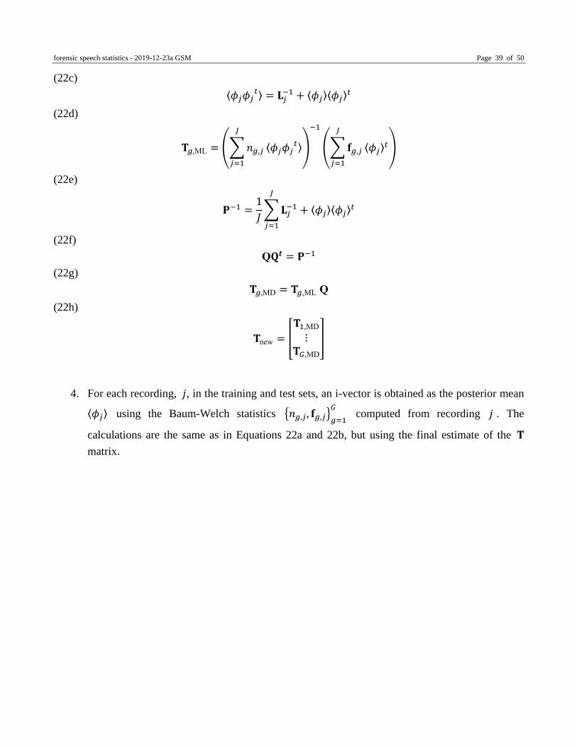
forensic speech statistics - 2019-12-23a GSM Page 39 of 50
(22c)
⟨𝜙𝑗𝜙𝑗𝑡⟩ = 𝐋𝑗
−1 + ⟨𝜙𝑗⟩⟨𝜙𝑗⟩𝑡
(22d)
𝐓𝑔,ML = (∑ 𝑛𝑔,𝑗
𝐽
𝑗=1
⟨𝜙𝑗𝜙𝑗𝑡⟩)
−1
(∑ 𝐟𝑔,𝑗
𝐽
𝑗=1
⟨𝜙𝑗⟩𝑡)
(22e)
𝐏−1 =1
𝐽∑ 𝐋𝑗
−1 + ⟨𝜙𝑗⟩⟨𝜙𝑗⟩𝑡
𝐽
𝑗=1
(22f)
Q𝐐𝒕 = 𝐏−1
(22g)
𝐓𝑔,MD = 𝐓𝑔,ML Q
(22h)
𝐓new = [
𝐓1,MD
⋮𝐓𝐺,MD
]
4. For each recording, 𝑗, in the training and test sets, an i-vector is obtained as the posterior mean
⟨𝜙𝑗⟩ using the Baum-Welch statistics {𝑛𝑔,𝑗 , 𝐟𝑔,𝑗}𝑔=1
𝐺 computed from recording 𝑗 . The
calculations are the same as in Equations 22a and 22b, but using the final estimate of the 𝐓
matrix.
forensic speech statistics - 2019-12-23a GSM Page 40 of 50
12 References
Ajili, M. 2017. Reliability of voice comparison for forensic applications. Doctoral Dissertation,
University of Avignon.
Aitken, C.G.G. and Lucy, D. 2004. Evaluation of trace evidence in the form of multivariate data.
Applied Statistics, 53: 109–122. http://dox.doi.org/10.1046/j.0035-9254.2003.05271.x
[Corrigendum: 2004. 53: 665–666. http://dox.doi.org/10.1111/j.1467-9876.2004.02031.x]
Arthur, D. and Vassilvitskii, S. 2007. k-means++: The advantages of careful seeding. In Proceedings of
the Eighteenth Annual ACM-SIAM Symposium on Discrete Algorithms, pp. 1027–1035.
Beritelli, F. and Spadaccini, A. 2011. The role of voice activity detection in forensic speaker
verification. In Proceedings of the 17th International Conference on Digital Signal Processing,
pp. 1–6. https://doi.org/10.1109/ICDSP.2011.6004980
Bogert, B.P., Healy, M.J.R., and Tukey, J.W. 1963. The quefrency alanysis of time series for echoes:
Cepstrum, pseudo autocovariance, cross-cepstrum and saphe cracking. In Rosenblatt, M. (ed),
Proceedings of the Symposium on Time Series Analysis, pp. 209–243. Wiley, New York.
Bousquet, P.-M., Bonastre, J.-F., and Matrouf, D. 2013. Identify the benefits of the different steps in an
i-vector based speaker verification system. In Progress in Pattern Recognition, Image Analysis,
Computer Vision, and Applications, pp. 278–285. Springer, Berlin.
http://dox.doi.org/10.1007/978-3-642-41827-3_35
Brümmer, N. and de Villiers, E. 2010. The speaker partitioning problem. In Proceedings of Odyssey
2010: The speaker and language recognition workshop, pp. 194–201. International Speech
Communication Association. https://www.isca-
speech.org/archive_open/odyssey_2010/od10_034.html
Brümmer, N. and du Preez, J. 2006. Application independent evaluation of speaker detection.
Computer Speech and Language, 20: 230–275. https://doi.org/10.1016/j.csl.2005.08.001
Chaudhary, G., Srivastava, S., and Bhardwaj, S. 2017. Feature extraction methods for speaker
recognition: A review. International Journal of Pattern Recognition and Artificial Intelligence,
31(12): 1750041-1–1750041-39. http://dx.doi.org/10.1142/S0218001417500410
Davis, S. and Mermelstein, P. 1980. Comparison of parametric representations for monosyllabic word
recognition in continuously spoken sentences. IEEE Transactions on Acoustics, Speech, and
Signal Processing, 28(4): 357–366. https://doi.org/10.1109/TASSP.1980.1163420
Dehak, N., Kenny, P.J., Dehak, R., Dumouchel, P., and Ouellet, P. 2011. Front-end factor analysis for
speaker verification. IEEE Transactions on Audio, Speech, and Language Processing, 19(4):
788–798. https://doi.org/10.1109/TASL.2010.2064307
Dempster, A.P., Laird, N.M., and Rubin D.B. 1977. Maximum likelihood from incomplete data via the
EM algorithm. Journal of the Royal Statistical Society, Series B, 39(1): 1–38.
http://www.jstor.org/stable/2984875
Dişken, G., Tüfekçi, Z., Saribulut, L., and Çevik, U. 2017. A review on feature extraction for speaker
recognition under degraded conditions. IETE Technical Review, 34(3): 321–332.
https://doi.org/10.1080/02564602.2016.1185976
Drygajlo, A., Jessen, M., Gfroerer, S., Wagner, I., Vermeulen, J., and Niemi, T. 2015. Methodological
guidelines for best practice in forensic semiautomatic and automatic speaker recognition,
forensic speech statistics - 2019-12-23a GSM Page 41 of 50
including guidance on the conduct of proficiency testing and collaborative exercises. European
Network of Forensic Science Institutes. http://enfsi.eu/wp-
content/uploads/2016/09/guidelines_fasr_and_fsasr_0.pdf
Duda, R.O., Hart, P.E., and Stork, D.G. 2000. Pattern Classification, 2nd edition. Wiley, New York.
Edmond, G., Towler, A., Growns, B., Ribeiro, G., Found, B., White, D., Ballantyne, K., Searston,
R.A., Thompson, M.B., Tangen, J.M., Kemp, R.I., and Martire K. 2017. Thinking forensics:
Cognitive science for forensic practitioners. Science & Justice, 57: 144–154.
http://dx.doi.org/10.1016/j.scijus.2016.11.005
Enzinger, E. 2014. A first attempt at compensating for effects due to recording-condition mismatch in
formant-trajectory-based forensic voice comparison. In Proceedings of the 15th Australasian
International Conference on Speech Science and Technology, pp. 133–136. Australasian Speech
Science and Technology Association. http://www.assta.org/sst/SST-14/6.A.%20
FORENSICS%202/1.%20ENZINGER.pdf
Enzinger, E. 2016. Implementation of forensic voice comparison within the new paradigm for the
evaluation of forensic evidence. Doctoral dissertation, University of New South Wales.
http://handle.unsw.edu.au/1959.4/55772
Enzinger, E. and Kasess, C.H. 2014. Bayesian vocal tract model estimates of nasal stops for speaker
verification. In Proceedings of the International Conference on Acoustics, Speech, and Signal
Processing (ICASSP 2014), pp. 1685–1689. http://dx.doi.org/10.1109/ICASSP.2014.6853885
Enzinger, E. and Morrison, G.S. 2017. Empirical test of the performance of an acoustic-phonetic
approach to forensic voice comparison under conditions similar to those of a real case. Forensic
Science International, 277: 30–40. http://dx.doi.org/10.1016/j.forsciint.2017.05.007
Enzinger, E., Zhang, C., and Morrison G.S. 2012. Voice source features for forensic voice comparison
– an evaluation of the Glottex® software package. In Proceedings of Odyssey 2012, The
Language and Speaker Recognition Workshop, pp. 78–85. International Speech Communication
Association. http://isca-speech.org/archive/odyssey_2012/od12_078.html [Errata and addenda
available at: https://box.entn.at/pdfs/enzinger2012_odyssey_vsferradd.pdf]
Fernández Gallardo, L. 2016. Human and Automatic Speaker Recognition over Telecommunication
Channels. Springer, Singapore. https://doi.org/10.1007/978-981-287-727-7
Ferrer, L., Nandwana, M.K., McLaren, M., Castan, D., and Lawson A. 2019. Toward fail-safe speaker
recognition: Trial-based calibration with a reject option. IEEE/ACM Transactions on Audio,
Speech, and Language Processing, 27: 140–153. http://dx.doi.org/10.1109/TASLP.2018.2875794
Fisher, R.A. 1936. The use of multiple measurements in taxonomic problems. Annals of Eugenics, 7:
179–188. http://dx.doi.org/10.1111/j.1469-1809.1936.tb02137.x
Forensic Science Regulator 2014. Guidance on validation (FSR-G-201 Issue 1). Forensic Science
Regulator, Birmingham, UK. https://www.gov.uk/government/publications/forensic-science-
providers-validation
Forensic Science Regulator 2016. Codes of Practice and Conduct – Appendix: Speech and Audio
Forensic Services (FSR-C-134 Issue 1). Forensic Science Regulator, Birmingham, UK.
https://www.gov.uk/government/publications/speech-and-audio-forensic-services
Forensic Science Regulator 2017. Codes of Practice and Conduct for forensic science providers and
practitioners in the Criminal Justice System (Issue 4). Forensic Science Regulator, Birmingham,
forensic speech statistics - 2019-12-23a GSM Page 42 of 50
UK. https://www.gov.uk/government/collections/forensic-science-providers-codes-of-practice-
and-conduct
Found, B. 2015. Deciphering the human condition: The rise of cognitive forensics. Australian Journal
of Forensic Sciences, 47: 386–401. http://dx.doi.org/10.1080/00450618.2014.965204
Fourier, J. 1808. Mémoire sur la propagation de la chaleur dans les corps solides, presented 21
December 1807 at the Institut national. Nouveau Bulletin des sciences par la Société
philomatique de Paris, 1(6): 112–116.
https://www.biodiversitylibrary.org/item/24789#page/120/mode/1up [Although the presentation
was given by Fourier, the published report of the presentation was written by Poisson.]
Furui, S. 1981. Cepstral analysis technique for automatic speaker verification. IEEE Transactions on
Acoustics, Speech, and Signal Processing, 29(2): 254–272.
https://doi.org/10.1109/TASSP.1981.1163530
Furui, S. 1986. Speaker-independent isolated word recognition using dynamic features of speech
spectrum. IEEE Transactions on Acoustics, Speech, and Signal Processing, 34: 52–59.
https://doi.org/10.1109/TASSP.1986.1164788
García-Romero, D. and Espy-Wilson, C.Y. 2011. Analysis of i-vector length normalization in speaker
recognition systems. In Proceedings of Interspeech 2011, pp. 249–252. International Speech
Communication Association. https://www.isca-
speech.org/archive/interspeech_2011/i11_0249.html
García-Romero, D. and McCree, A. 2014. Supervised domain adaptation for i-vector based speaker
recognition. In Proceeding of the IEEE International Conference on Acoustics, Speech, and
Signal Processing, pp. 4828–4831. http://dx.doi.org/10.1109/ICASSP.2014.6854362
García-Romero, D. and McCree, A. 2015. Insights into deep neural networks for speaker recognition.
In Proceedings of Interspeech 2015, pp. 1141–1145. International Speech Communication
Association. https://www.isca-speech.org/archive/interspeech_2015/i15_1141.html
Garcia-Romero, D., Zhang, X., McCree, A., and Povey, D. 2014. Improving speaker recognition
performance in the domain adaptation challenge using deep neural networks. In Proceedings of
the 2014 IEEE Spoken Language Technology Workshop (SLT), pp. 378–383.
Glembek, O. 2012. Optimization of Gaussian mixture subspace models and related scoring algorithms
in speaker verification. Doctoral dissertation, Brno University of Technology.
González-Rodríguez, J., Rose, P., Ramos, D., Toledano, D.T., and Ortega-García, J. 2007. Emulating
DNA: Rigorous quantification of evidential weight in transparent and testable forensic speaker
recognition. IEEE Transactions on Audio, Speech, and Language Processing, 15: 2104–2115.
https://doi.org/10.1109/TASL.2007.902747
Hansen, J.H.L. and Bořil, H. 2018. On the issues of intra-speaker variability and realism in speech,
speaker, and language recognition tasks. Speech Communication, 101: 94–108.
https://doi.org/10.1016/j.specom.2018.05.004
Hansen, J.H.L. and Hasan, T. 2015. Speaker recognition by machines and humans: A tutorial review.
IEEE Signal Processing Magazine, November 74–99.
http://dx.doi.org/10.1109/MSP.2015.2462851
Harris, F.J. 1978. On the use of windows for harmonic analysis with the discrete Fourier transform.
Proceedings of the IEEE, 66(1): 51–83. http://dx.doi.org/10.1109/PROC.1978.10837

forensic speech statistics - 2019-12-23a GSM Page 43 of 50
Hastie, T., Tibshirani, R., and Freidman, J. 2009. The Elements of Statistical Learning Data Mining,
Inference, and Prediction, 2nd edition. Springer, New York.
Hosmer, D.W. Jr., Lemeshow, S., and Sturdivant, R.X. 2013. Applied Logistic Regression, 3rd edition.
Wiley, Hoboken NJ. http://dx.doi.org/10.1002/9781118548387
Hwang, M.Y. and Huang, X. 1992. Subphonetic modeling with Markov states – Senone. In
Proceedings of the IEEE International Conference on Acoustics, Speech, and Signal Processing
(ICASSP), pp. I-33–I-36. https://doi.org/10.1109/ICASSP.1992.225979
Jessen, M., Alexander, A., and Forth O. 2014. Forensic voice comparisons in German with phonetic
and automatic features using Vocalise software. In: Proceedings of the 54th Audio Engineering
Society (AES) Forensics Conference, pp. 28–35. Audio Engineering Society.
Kelly, F. and Hansen, J.H.L. 2016. Score-aging calibration for speaker verification. IEEE/ACM
Transactions on Audio, Speech, and Language Processing, 24, 2414–2424.
http://dx.doi.org/10.1109/TASLP.2016.2602542
Kenny, P. 2005. Joint factor analysis of speaker and session variability: Theory and algorithms.
Technical Report CRIM-06/08-13. Centre de Recherche Informatique de Montréal.
Kenny, P., Boulianne G., and Dumouchel P. 2005. Eigenvoice modeling with sparse training data.
IEEE Transaction on Speech and Audio Processing, 13, 345–354.
https://doi.org/10.1109/TSA.2004.840940
Kenny, P. 2010. Bayesian speaker verification with heavy tailed priors. In Proceedings of Odyssey
2010: The Speaker and Language Recognition Workshop, paper 014. International Speech
Communication Association. https://www.isca-
speech.org/archive_open/odyssey_2010/od10_014.html
Kenny, P., Gupta, V., Stafylakis, T., Ouellet, P., and Alam, J. 2014. Deep neural networks for
extracting Baum-Welch statistics for speaker recognition. In Proceedings of Odyssey 2014, pp.
293–298. International Speech Communication Association. https://www.isca-
speech.org/archive/odyssey_2014/abstracts.html#abs28
Kinnunen, T. and Li, H. 2010. An overview of text-independent speaker recognition: From features to
supervectors. Speech Communication, 52: 12–40.
http://dx.doi.org/10.1016/j.specom.2009.08.009
Klecka, W.R. 1980. Discriminant Analysis. Sage, Beverly Hills, CA.
Lei, Y., Scheffer, N., Ferrer, L., and McLaren, M. 2014. A novel scheme for speaker recognition using
a phonetically-aware deep neural network. In Proceedings of the 2014 IEEE International
Conference on Acoustics, Speech and Signal Processing (ICASSP), pp. 1695–1699.
https://doi.org/10.1109/ICASSP.2014.6853887
Lozano-Díez, A., Silnova, A., Matějka, P., Glembek, O., Plchot, O., Pesan, J., Burget, L., and
González-Rodríguez, J. 2016. Analysis and Optimization of Bottleneck Features for Speaker
Recognition. In Proceedings of Odyssey 2016, pp. 352–357. International Speech
Communication Association. http://dx.doi.org/10.21437/Odyssey.2016-51
Lucy, D. 2005. Introduction to Statistics for Forensic Scientists. Wiley, Chichester, UK.
Mandasari, M.I., McLaren, M., and van Leeuwen, D.A. 2012. The effect of noise on modern automatic
speaker recognition systems. In Proceedings of the 2012 IEEE International Conference on
forensic speech statistics - 2019-12-23a GSM Page 44 of 50
Acoustics, Speech and Signal Processing (ICASSP), pp. 4249–4252.
https://doi.org/10.1109/ICASSP.2012.6288857
Mandasari, M.I., Saeidi, R., McLaren, M., and van Leeuwen, D.A. 2013. Quality measure functions for
calibration of speaker recognition systems in various duration conditions. IEEE Transactions on
Audio, Speech, and Language Processing, 21: 2425–2438.
http://dx.doi.org/10.1109/TASL.2013.2279332
Mandasari, M.I., Saeidi, R., and van Leeuwen, D.A. 2015. Quality measures based calibration with
duration and noise dependency for speaker recognition. Speech Communication, 72: 126–137.
http://dx.doi.org/10.1016/j.specom.2015.05.009
Matějka P., Glembek O., Castaldo F., Alam M., Plchot O., Kenny P., Burget L., and Černocky J., 2011.
Full-covariance UBM and heavy-tailed PLDA in i-vector speaker verification. In Proceeding of
the 2011 IEEE International Conference on Acoustics, Speech, and Signal Processing (ICASSP),
pp. 4828–4831. http://dx.doi.org/10.1109/ICASSP.2011.5947436
Matějka, P., Glembek, O., Nomotiv, O., Plchot, O., Grézl, F., Burget, L., and Černocky, J. 2016.
Analysis of DNN approaches to speaker identification. In Proceeding of the 2016 IEEE
International Conference on Acoustics, Speech, and Signal Processing (ICASSP), pp. 5100–
5104. http://dx.doi.org/ 10.1109/ICASSP.2016.7472649
Matrouf, D., Scheffer, N., Fauve, B., and Bonastre, J. 2007. A straightforward and efficient
implementation of the factor analysis model for speaker verification. In Proceedings of
Interspeech, pp. 1242–1245. International Speech Communication Association. https://www.isca-
speech.org/archive/interspeech_2007/i07_1242.html
McLaren, M, Lawson, A., Ferrer, L., Scheffer, N., and Lei, Y. 2014. Trial-based calibration for speaker
recognition in unseen conditions. In Proceedings of Odyssey 2014: The Speaker and Language
Recognition Workshop, pp. 19–25. International Speech Communication Association.
https://www.isca-speech.org/archive/odyssey_2014/abstracts.html#abs43
Menard, S. 2010. Logistic Regression: From Introductory to Advanced Concepts and Applications.
Sage, Thousand Oaks, CA. http://dx.doi.org/10.4135/9781483348964
Meuwly, D. 2001. Reconnaissance de locuteurs en sciences forensiques: l’apport d’une approche
automatique [Speaker recognition in forensic science: The contribution of an automatic
approach]. Doctoral dissertation, University of Lausanne.
Meuwly, D., Ramos, D., and Haraksim R. 2017. A guideline for the validation of likelihood ratio
methods used for forensic evidence evaluation, Forensic Science International, 276: 142–153.
http://dx.doi.org/10.1016/j.forsciint.2016.03.048
Morrison, G.S. 2011. Measuring the validity and reliability of forensic likelihood-ratio systems.
Science & Justice, 51: 91–98. http://dx.doi.org/10.1016/j.scijus.2011.03.002
Morrison, G.S. 2013. Tutorial on logistic-regression calibration and fusion: Converting a score to a
likelihood ratio. Australian Journal of Forensic Sciences, 45: 173–197.
http://dx.doi.org/10.1080/00450618.2012.733025
Morrison, G.S. 2014. Distinguishing between forensic science and forensic pseudoscience: Testing of
validity and reliability, and approaches to forensic voice comparison. Science & Justice, 54: 245–
256. http://dx.doi.org/10.1016/j.scijus.2013.07.004
forensic speech statistics - 2019-12-23a GSM Page 45 of 50
Morrison, G.S. 2018a. Admissibility of forensic voice comparison testimony in England and Wales.
Criminal Law Review, 2018(1): 20–33.
Morrison, G.S. 2018b. The impact in forensic voice comparison of lack of calibration and of
mismatched conditions between the known-speaker recording and the relevant-population sample
recordings. Forensic Science International, 283: e1–e7.
http://dx.doi.org/10.1016/j.forsciint.2017.12.024
Morrison, G.S. and Enzinger, E. 2016. Multi-laboratory evaluation of forensic voice comparison
systems under conditions reflecting those of a real forensic case (forensic_eval_01) -
Introduction. Speech Communication, 85: 119–126.
http://dx.doi.org/10.1016/j.specom.2016.07.006
Morrison, G.S. and Enzinger, E. 2018. Score based procedures for the calculation of forensic likelihood
ratios – Scores should take account of both similarity and typicality. Science & Justice, 58: 47–
58. http://dx.doi.org/10.1016/j.scijus.2017.06.005
Morrison, G.S. and Enzinger, E. 2019. Forensic voice comparison. In Katz, W.F. and Assmann, P.F.
(eds.), The Routledge Handbook of Phonetics, pp. 599–634. Routledge, Abingdon, UK.
https://doi.org/10.4324/9780429056253
Morrison, G.S., Enzinger, E., and Zhang, C. 2018. Forensic speech science. In Freckelton, I. and Selby,
H. (eds.), Expert Evidence, ch. 99. Thomson Reuters, Sydney, Australia.
Morrison, G.S. and Poh, N. 2018. Avoiding overstating the strength of forensic evidence: Shrunk
likelihood ratios / Bayes factors. Science & Justice, 58: 200–218.
http://dx.doi.org/10.1016/j.scijus.12.005
Morrison, G.S. and Stoel, R.D. 2014. Forensic strength of evidence statements should preferably be
likelihood ratios calculated using relevant data, quantitative measurements, and statistical models
– a response to Lennard (2013) Fingerprint identification: How far have we come? Australian
Journal of Forensic Sciences, 46: 282–292. http://dx.doi.org/10.1080/00450618.2013.833648
Morrison, G.S. and Thompson, W.C. 2017. Assessing the admissibility of a new generation of forensic
voice comparison testimony. Columbia Science and Technology Law Review, 18: 326–434.
National Commission on Forensic Science 2015. Ensuring that forensic analysis is based upon task-
relevant information. https://www.justice.gov/ncfs/file/818196/download
Ommen, D.M. and Saunders, C.P. 2018. Building a unified statistical framework for the forensic
identification of source problems. Law, Probability and Risk. 17: 179–197.
http://dx.doi.org/10.1093/lpr/mgy008
Peddinti, V., Chen, G., Povey, D., Khudanpur, S. 2015. Reverberation robust acoustic modeling using
i-vectors with time delay neural networks. In Proceedings of Interspeech 2015, pp. 2440–2444.
International Speech Communication Association. https://www.isca-
speech.org/archive/interspeech_2015/i15_2440.html
Peddinti, V., Povey, D., Khudanpur, S. 2015. A time delay neural network architecture for efficient
modeling of long temporal contexts. In Proceedings of Interspeech 2015, pp. 3214–3218.
International Speech Communication Association. https://www.isca-
speech.org/archive/interspeech_2015/i15_3214.html

forensic speech statistics - 2019-12-23a GSM Page 46 of 50
Pelecanos, J. and Sridharan, S. 2001. Feature warping for robust speaker verification. In Proceedings of
Odyssey 2001: The Speaker Recognition Workshop, pp. 213–218. International Speech
Communication Association. https://www.isca-speech.org/archive_open/odyssey/odys_213.html
Pearson, K. 1901. On lines and planes of closest fit to systems of points in space. The London,
Edinburgh, and Dublin Philosophical Magazine and Journal of Science, Series 6, 2(11): 559–
572. http://dx.doi.org/10.1080/14786440109462720
Pigeon, S., Druyts, P., and Verlinde, P. 2000. Applying logistic regression to the fusion of the NIST’99
1-speaker submissions. Digital Signal Processing, 10: 237–248. http://dx.doi.org/10.1006/
dspr.1999.0358
President’s Council of Advisors on Science and Technology 2016. Forensic Science in Criminal
Courts: Ensuring Scientific Validity of Feature-Comparison Methods. https://obamawhitehouse.
archives.gov/administration/eop/ostp/pcast/docsreports/
Prince, S.J.D. and Elder, J.H. 2007. Probabilistic linear discriminant analysis for inferences about
identity. In Proceedings of the IEEE 11th International Conference on Computer Vision, pp. 1–8.
https://doi.org/10.1109/ICCV.2007.4409052
Ramos Castro, D. 2007. Forensic evaluation of the evidence using automatic speaker recognition
systems. Doctoral dissertation, Autonomous University of Madrid.
Reynolds, D.A. 1994. Speaker identification and verification using Gaussian mixture speaker models.
In Proceedings of the ESCA Workshop on Automatic Speaker Recognition, Identification, and
Verification, pp. 27–30.
Reynolds, D.A., Quatieri, T.F., and Dunn, R.B. 2000. Speaker verification using adapted Gaussian
mixture models. Digital Signal Processing, 10: 19–41. https://doi.org/10.1006/dspr.1999.0361
Sadjadi, S.O. and Hansen, J.H.L. 2013. Unsupervised speech activity detection using voicing measures
and perceptual spectral flux. IEEE Signal Processing Letters, 20(3): 197–200.
https://doi.org/10.1109/LSP.2013.2237903
Silva, D.G. and Medina, C.A. 2017. Evaluation of MSR Identity Toolbox under conditions reflecting
those of a real forensic case (forensic_eval_01). Speech Communication, 94: 42–49.
http://dx.doi.org/10.1016/j.specom.2017.09.001
Sizov, A., Lee, K.A., and Kinnunen, T. 2014. Unifying probabilistic linear discriminant analysis
variants in biometric authentication. In Fränti, P., Brown, G., Loog, M. Escolano, F. and Pelillo,
M. editors, Structural, Syntactic, and Statistical Pattern Recognition, pp. 464–475. Springer,
Berlin. https://doi.org/10.1007/978-3-662-44415-3_47
Snyder, D., Garcia-Romero, D., Povey, D., and Khudanpur, S. 2017. Deep neural network embeddings
for text-independent speaker verification. In Proceedings of Interspeech 2017, pp. 999–1003.
International Speech Communication Association. http://dx.doi.org/10.21437/Interspeech.2017-
620
Snyder, D., Garcia-Romero, D., Sell, G., Povey, D., and Khudanpur, S. 2018. X-vectors: Robust DNN
embeddings for speaker recognition. In Proceedings of IEEE International Conference on
Acoustics, Speech and Signal Processing (ICASSP) 2018, pp. 5329–5333.
http://dx.doi.org/10.1109/ICASSP.2018.8461375
Sohn, J., Kim, N.S., and Sung, W. 1999. A statistical model-based voice activity detection. IEEE
Signal Processing Letters, 6(1): 1–3. https://doi.org/10.1109/97.736233
forensic speech statistics - 2019-12-23a GSM Page 47 of 50
Stevens, S.S., Volkmann, J., and Newman, E.B. 1937. A scale for the measurement of the
psychological magnitude pitch. Journal of the Acoustical Society of America, 8: 185–190.
https://doi.org/10.1121/1.1915893
Stoel, R.D., Berger, C.E.H., Kerkhoff, W., Mattijssen, E.J.A.T., and Dror E.I. 2015. Minimizing
contextual bias in forensic casework. In Strom K.J. and Hickman M.J. (eds.), Forensic Science
and the Administration of Justice: Critical Issues and Directions, pp. 67–86. Sage, Thousand
Oaks, CA. http://dx.doi.org/10.4135/9781483368740.n5
Tirumala, S.S., Shahamiri, S. R., Garhwal, A.S., and Wang, R. 2017. Speaker identification features
extraction methods: A systematic review. Expert Systems with Applications, 90: 250–271.
https://doi.org/10.1016/j.eswa.2017.08.015
Ueda, N., Nakano, R., Ghahramani, Z., and Hinton, G.E. 2000. Split and merge EM algorithm for
improving Gaussian mixture density estimates. The Journal of VLSI Signal Processing-Systems
for Signal, Image, and Video Technology, 26: 133–140.
http://dx.doi.org/10.1023/A:1008155703044
Viikki, O. and Laurila, K. 1998. Cepstral domain segmental feature vector normalization for noise
robust speech recognition. Speech Communication, 25: 133–147. https://doi.org/10.1016/S0167-
6393(98)00033-8
Wilson-Wilde, L. 2018. The international development of forensic science standards: A review.
Forensic Science International, 288: 1–9. https://doi.org/10.1016/j.forsciint.2018.04.009
Yaman, S., Pelecanos, J., and Sarikaya, R. 2012. Bottleneck features for speaker recognition. In
Proceedings of Odyssey 2012, pp. 105–108. International Speech Communication Association.
https://www.isca-speech.org/archive/odyssey_2012/od12_105.html
Zhang, C., Morrison, G.S., Enzinger, E., and Ochoa F. 2013. Effects of telephone transmission on the
performance of formant-trajectory-based forensic voice comparison – female voices. Speech
Communication, 55: 796–813. http://dx.doi.org/10.1016/j.specom.2013.01.011
Legal references
Criminal Practice Directions [2015] EWCA Crim 1567
Daubert v. Merrell Dow Pharms., 509 U.S. 579 (1993)
Federal Rules of Evidence as amended Apr. 17, 2000, eff. Dec. 1, 2000; Apr. 26, 2011, eff. Dec. 1,
2011.
General Electric Co. v. Joiner, 522 U.S. 136 (1997)
Kumho Tire Co. v. Carmichael, 526 U.S. 137 (1999)

forensic speech statistics - 2019-12-23a GSM Page 48 of 50
13 Figure captions
Figure 1. Procedure for the calculation of MFCCs. The numbers in black circles correspond to the
numbered steps in the main text. DFT = discrete Fourier transform. DCT = discrete cosine transform.
Figure 2. Feature warping. The original feature value is replaced by the warped feature value. The
warping is achieved by mapping from the empirical cumulative probability distribution of the original
feature values to a parametric target cumulative probability distribution, in this case the standard
cumulative Gaussian distribution.
Figure 3. Examples of the effects of channel and feature warping on the distribution of MFCCs. The first
column represents MFCC values extracted from a high-quality audio signal (the same in both rows). The
next three columns represent the results of sequentially applying various signal processing techniques to
simulate casework conditions. The top row represents a simulated questioned-speaker recording
condition and the bottom row represents a simulated known-speaker recording condition. The final
column represents the results of applying feature warping to the values represented in the immediately
preceding column, applied separately to the simulated questioned-speaker recording condition and to the
simulated known-speaker recording condition.
Figure 4. Example of using the EM algorithm to train a two-component GMM. The example is based on
artificial data that were created for illustrative purposes. The dotted curve represents the distribution that
was used to generate the data. The dashed curve represents the fitted GMM, and the black curve and the
white curve represent the two Gaussian components of the fitted GMM. The top panel shows the initial
GMM distribution based on a random seed. The data points (the circles on the x axis) are shaded
according to their responsibilities with respect to the two components. The second panel shows the fitted
GMM distribution after 1 iteration of maximization (along with the responsibilities after that iteration).
The third panel shows the results after 20 iterations, and the bottom panel the results after 40 iterations.
Figure 5. Example of using a GMM-UBM model to calculate a likelihood ratio for a single questioned-
speaker-recording feature vector. This example is based on artificial two-dimensional data generated for
illustrative purposes. The UBM is represented by the surface drawn with the darker mesh and the MAP
adapted known-speaker GMM is represented by the surface drawn with the lighter mesh. The x-y location
of the vertical line indicates a questioned-speaker-recording feature vector value at which the likelihoods
of the UBM and the known-speaker GMM are being evaluated (the likelihoods are given by the z values
forensic speech statistics - 2019-12-23a GSM Page 49 of 50
of the intersections of the vertical line with each of the surfaces).
Figure 6. Example of using PCA to reduce the data from two dimensions to one dimension. The example
uses artificial data created for illustrative purposes. Different shaped symbols represent different speakers
and the two different intensities of shading represent two different conditions, e.g., a questioned-speaker-
recording condition and a known-speaker-recording condition. The PCA dimension (represented by the
oblique axis) is in the direction of maximum variance in the original x-y space.
Figure 7. Example of using CLDF for mismatch compensation and to reduce the data from two
dimensions to one dimension. The example uses artificial data created for illustrative purposes (the same
data as used for Figures 6). Different shaped symbols represent different speakers and the two different
intensities of shading represent two different conditions, e.g., a questioned-speaker-recording condition
and a known-speaker-recording condition. The CLDF dimension (represented by the oblique axis) is in
the direction in the original x-y space that has the maximum ratio of between- versus within-speaker
variance.
Figure 8. Example of using a PLDA model to calculate a score for a pair of i-vectors. The numerator of
the PLDA model is represented by the surface drawn with the lighter mesh and the denominator is
represented by the surface drawn with the darker mesh. The x-y location of the vertical line indicates the
values of the i-vectors 𝑣𝑞 and 𝑣𝑘 (extracted from the questioned- and known -speaker recordings
respectively) at which the likelihoods of numerator and denominator of the PLDA model are being
evaluated (the likelihoods are given by the z values of the intersections of the vertical line with each of
the surfaces).
Figure 9. Simplified example of the architecture of a feed-forward DNN consisting of an input layer,
two hidden layers, and an output layer. Not all connection between nodes have been drawn, and weights
have been indicated for only a few connections.
Figure 10. Illustration of the architecture of a DNN embedding system. Only the time-dimension is
shown for the frame level (the frequency dimension is not shown). The input layer (at the bottom) spans
t–7 through t+7. The time dimension is collapsed by the third hidden layer of the frame level. The
statistics-pooling layer calculates the mean and standard deviation of each node in the preceding layer
when the whole of the speech of interest in a recording is passed by the input layer. The frequency
dimension is shown for the segment level.
forensic speech statistics - 2019-12-23a GSM Page 50 of 50
Figure 11. Example of using linear discriminant analysis or logistic regression to convert a score to a
likelihood ratio. The example uses artificial data created for illustrative purposes. Different-speaker
training scores are shown as grey triangles and same-speaker training scores are shown as white circles.
The top panel shows a linear discriminant analysis model fitted to the data. The middle and bottom panels
can be derived from the top panel. The middle and bottom panels can also be derived by fitting a logistic
regression model to the same data. The vertical line represents a score value that is being converted to a
likelihood-ratio value. In the top panel the output is clearly the ratio of two likelihoods. The middle panel
shown that the conversion from scores to log-likelihood-ratio values is a linear function. (In reality the
plotted training data are illustrative only and the plotted functions show ideal values based on specified
parametric distributions.)
Figure 12. Penalty functions for calculating Cllr. The same-speaker and different-speaker curves
correspond to the functions within Equation 20’s left and right summations respectively.
Figure 13. Examples of Tippett plots. The three plots represent three different systems tested on the same
test data. The examples are based on artificial data created for illustrative purposes. The data represent
50 same-speaker test pairs and 200 different-speaker test pairs – imbalance in the number of same-
speaker and different-speaker test pairs is usual since it is easier to construct different-speaker pairs than
same-speaker pairs. The Cllr values corresponding to the results shown in the top, middle, and bottom
panels are 1.068, 0.698, and 0.307 respectively.

time
inte
nsi
ty
frequency (Hz)
inte
nsi
ty
DFT
frequency (Hz)
inte
nsi
ty
× logfrequency (mel)lo
g i
nte
nsi
ty
frequency (mel)log
in
ten
sity
1st MFCC
2nd MFCC
3rd MFCC
4th MFCC
5th MFCC
DCT
windowing
power spectrum
speech signal
mel filterbank
filterbank output
fitted DCT
DCT coefficient values
�
�
�
�
�
�

0
0.2
0.4
0.6
0.8
1
MFCC value
cdis
trib
ution
um
ula
tive
−10 −8 −6 −4 −2 0 2 4 6 8
empirical
target
origin
al
warp
ed

high quality
0 +5 +10-5-10
reverberation
0 +5 +10-5-10
MPEG 2 layer 1 compression
0 +5 +10-5-10
background ventilation noise
0 +5 +10-5-10
after feature warping
0 +1 +2-1-2
after feature warpingbackground babble noiseG.732.1 compressionlandline bandpasshigh quality

0
0.05
0.1
0.15
0.2
0.25
0.3pr
obab
ility
den
sity
0
0.05
0.1
0.15
0.2
0.25
0.3
prob
abili
ty d
ensi
ty
0
0.05
0.1
0.15
0.2
0.25
0.3
prob
abili
ty d
ensi
ty
-8 -6 -4 -2 0 2 4 60
0.05
0.1
0.15
0.2
0.25
0.3
prob
abili
ty d
ensi
ty

F1F2
0
1980
1990 380
2000 390
0.5
4002010
4102020
4202030
prob
abili
ty d
ensi
ty
#10-3
4302040
1
440
1.5

0
0.1
0.2
0.3
pro
ba
bili
ty d
en
sity
0
0.1
0.2
0.3
prob
abilit
y de
nsity
-4 -3 -2 -1 0 1 2 3 4
-4
-3
-2
-1
0
1
2
3
4
x
y
0
0.1
0.2
0.3
probability density

0
0.2
5
0.5
0.7
5 1
1.2
5
probability density
00.25
0.50.75
11.25
pro
babili
ty d
ensity
0
0.25
0.5
0.75
1
1.25
pro
ba
bili
ty d
en
sity
-4 -3 -2 -1 0 1 2 3 4
-4
-3
-2
-1
0
1
2
3
4
x
y
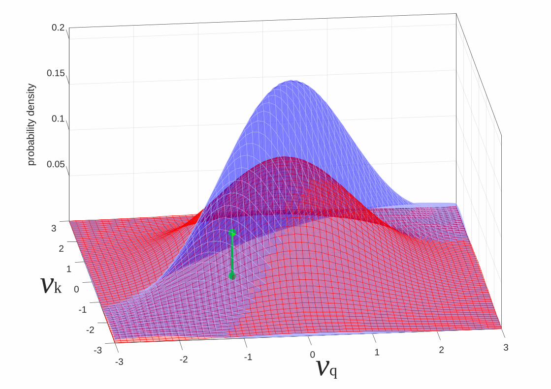
vq
vk
3
0.05
2
0.1
prob
abili
ty d
ensi
ty
1
0.15
0.2
0
-1
-2
32-3 10-1-2-3
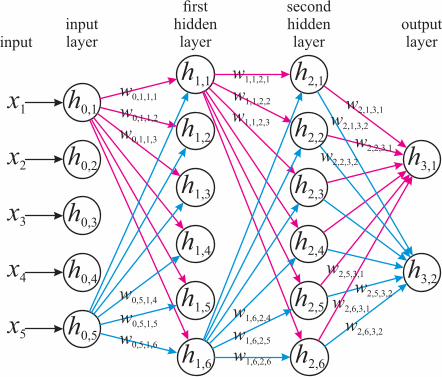
h1,1
h1,2
h1,3
h1,4
h1,5
h0,1
h0,2
h0,3
h0,4
h0,5
h1,6
h2,1
h2,2
h2,3
h2,4
h2,5
h2,6
w1,1,2,1
w1,1,2,2
w1,1,2,3
w1,6,2,4
w1,6,2,5
w1,6,2,6
w0,1,1,1
w0,1,1,2
w0,1,1,3
w0,5,1,6
w0,5,1,5
w0,5,1,4
h3,1
h3,2
w2,1,3,1
w2,1,3,2
w2,2,3,1
w2,6,3,2
w2,6,3,1
w2,5,3,2
inputlayer
firsthiddenlayer
secondhiddenlayer
outputlayer
x1
x2
x3
x4
x5
input
w2,2,3,2
w2,5,3,1

output layer
embedding
embedding
segm
ent le
vel
fram
e level
statistics pooling μ σ
t +2t +1 +3 +4 +5 +6 +7-1-2-3-4-5-6-7

0
0.1
0.2
0.3
0.4
prob
abili
ty d
ensi
ty
-4
-2
0
2
4
log(
LR)
-4 -3 -2 -1 0 1 2 3 4
score
0
0.2
0.4
0.6
0.8
1
prob
abili
ty

Log Likelihood Ratio10
penalty v
alu
e
-3 -2 -1 0 1 2
1
2
3
4
5
6
7
8
9
3
same-speaker function
diffe
rent
-spe
aker
func
tion

0
0.1
0.2
0.3
0.4
0.5
0.6
0.7
0.8
0.9
1C
um
ula
tive P
roport
ion
0
0.1
0.2
0.3
0.4
0.5
0.6
0.7
0.8
0.9
1
Cum
ula
tive P
roport
ion
-4 -3 -2 -1 0 1 2 3 4
Log10 Likelihood Ratio
0
0.1
0.2
0.3
0.4
0.5
0.6
0.7
0.8
0.9
1
Cum
ula
tive P
roport
ion