Statistical Modeling of Carbon Dioxide and Cluster ...
107
University of South Florida Scholar Commons Graduate eses and Dissertations Graduate School 6-2-2016 Statistical Modeling of Carbon Dioxide and Cluster Analysis of Time Dependent Information: Lag Target Time Series Clustering, Multi-Factor Time Series Clustering, and Multi-Level Time Series Clustering Doo Young Kim University of South Florida, [email protected] Follow this and additional works at: hp://scholarcommons.usf.edu/etd Part of the Environmental Sciences Commons , Medicine and Health Sciences Commons , and the Statistics and Probability Commons is esis is brought to you for free and open access by the Graduate School at Scholar Commons. It has been accepted for inclusion in Graduate eses and Dissertations by an authorized administrator of Scholar Commons. For more information, please contact [email protected]. Scholar Commons Citation Kim, Doo Young, "Statistical Modeling of Carbon Dioxide and Cluster Analysis of Time Dependent Information: Lag Target Time Series Clustering, Multi-Factor Time Series Clustering, and Multi-Level Time Series Clustering" (2016). Graduate eses and Dissertations. hp://scholarcommons.usf.edu/etd/6277
Transcript of Statistical Modeling of Carbon Dioxide and Cluster ...

University of South FloridaScholar Commons
Graduate Theses and Dissertations Graduate School
6-2-2016
Statistical Modeling of Carbon Dioxide and ClusterAnalysis of Time Dependent Information: LagTarget Time Series Clustering, Multi-Factor TimeSeries Clustering, and Multi-Level Time SeriesClusteringDoo Young KimUniversity of South Florida, [email protected]
Follow this and additional works at: http://scholarcommons.usf.edu/etd
Part of the Environmental Sciences Commons, Medicine and Health Sciences Commons, andthe Statistics and Probability Commons
This Thesis is brought to you for free and open access by the Graduate School at Scholar Commons. It has been accepted for inclusion in GraduateTheses and Dissertations by an authorized administrator of Scholar Commons. For more information, please contact [email protected].
Scholar Commons CitationKim, Doo Young, "Statistical Modeling of Carbon Dioxide and Cluster Analysis of Time Dependent Information: Lag Target TimeSeries Clustering, Multi-Factor Time Series Clustering, and Multi-Level Time Series Clustering" (2016). Graduate Theses andDissertations.http://scholarcommons.usf.edu/etd/6277

Statistical Modeling of Carbon Dioxide and Cluster Analysis of Time Dependent Information:
Lag Target Time Series Clustering, Multi-Factor Time Series Clustering,
and Multi-Level Time Series Clustering
by
Doo Young Kim
A dissertation submitted in partial fulfillment of the requirements for the degree of
Doctor of Philosophy Department of Mathematics & Statistics
College of Arts and Sciences University of South Florida
Major Professor: Chris P. Tsokos, Ph.D. Kandethody Ramachandran, Ph.D.
Lu Lu, Ph.D.��Sanghoon Park, Ph.D
Date of Approval: May 31, 2016
Keywords: Global Warming, Transitional Modeling, Clustering, Time Dependent Information, Cancer Mortality Rates
Copyright ©2016, Doo Young Kim

Dedication
This doctoral dissertation is dedicated to my parents (Se-ung Joo Kim and Dong Ok Bae), parents-in-law (ChangBeom Shin and Young Sook Ahn), my wife (Juhee Shin),my daughters (Minji Kim and Sage H. Kim), and mybrother-in-law (Yongwoo Shin).

Acknowledgments
I would like to express my deepest appreciation to my major professor, Dr. Chris P. Tsokos,
for being a big tree for me. He has protected me from heavy rains and allowed me to take
academic nutritions in his arms which motivated me to find the right way to proceed during my
graduate study at the University of South Florida. Following his life is now the goal of my life
and I believe it is the only way to return all his mentoring.
I would like to thank to Dr. Kandethody Ramachandran for being a good example of a professor
and supporting me as a member of my Ph.D. committee for my whole candidacy period. Also,
I would like to thank to Dr. Rebecca Wooten for serving as a former member of my Ph.D.
committee and supporting me for a long time. Lastly, I am also thankful to Dr. Lu Lu and Dr.
Sanghoon Park for being members of my Ph.D. committee.
Furthermore, many thanks to all my friends who have always encouraged me to study hard
and gave me self-confidence: Dr. Ram Kafle, Dr. Bong-Jin Choi, Bhikhari Tharu, A. K. M. R
Bashar, and all my other friends that are not listed.
Finally, I was not able to reach this point without the endless support of my beloved wife, Juhee
Shin. She has always supported and encouraged me to do my best without any complaint in
any situation. My great thanks to Juhee for being the best wife and the best mom for our lovely
children, Minji and Sage.

Table of Contents
List of Tables . . . . . . . . . . . . . . . . . . . . . . . . . . . . . . . . . . . . . . . . . . . iii
List of Figures . . . . . . . . . . . . . . . . . . . . . . . . . . . . . . . . . . . . . . . . . . . v
Abstract . . . . . . . . . . . . . . . . . . . . . . . . . . . . . . . . . . . . . . . . . . . . . . vii
Chapter 1 Introduction . . . . . . . . . . . . . . . . . . . . . . . . . . . . . . . . . . . . . 11.1 Statistical Modeling of the Carbon Dioxide in the Atmosphere . . . . . . . . . . . . 1
1.1.1 Components in Statistical Modeling . . . . . . . . . . . . . . . . . . . . . . 11.1.2 Atmospheric CO2 in South Korea, United States, and European Union . . . . 3
1.2 Regional Analysis of the Atmospheric Carbon Dioxide in the United States . . . . . 41.2.1 Statistical Modeling . . . . . . . . . . . . . . . . . . . . . . . . . . . . . . 4
1.3 New Methods to Cluster Time Dependent Information . . . . . . . . . . . . . . . . 51.3.1 Lag Target Time Series Clustering (LTTC) and Multi-Factor Time Series
Clustering (MFTC) Methods . . . . . . . . . . . . . . . . . . . . . . . . . . 51.3.2 Multi-Level Time Series Clustering (MLTC) Method . . . . . . . . . . . . . 6
Chapter 2 Statistical Significance of Fossil Fuels Contributing to Atmospheric Carbon Dioxidein South Korea and Comparisons with USA and EU . . . . . . . . . . . . . . . . . . . . . 72.1 Introduction . . . . . . . . . . . . . . . . . . . . . . . . . . . . . . . . . . . . . . . 72.2 Materials and Methods . . . . . . . . . . . . . . . . . . . . . . . . . . . . . . . . . 10
2.2.1 Data . . . . . . . . . . . . . . . . . . . . . . . . . . . . . . . . . . . . . . . 102.2.2 Statistical Modeling . . . . . . . . . . . . . . . . . . . . . . . . . . . . . . 11
2.3 Results and Discussion . . . . . . . . . . . . . . . . . . . . . . . . . . . . . . . . . 152.3.1 Ranking of the Contributing Variables - South Korea . . . . . . . . . . . . . 152.3.2 Ranking of the Contributing Variables - United States . . . . . . . . . . . . . 152.3.3 Ranking of the Contributing Variables - European Union . . . . . . . . . . . 162.3.4 Comparison: U.S., EU, and South Korea . . . . . . . . . . . . . . . . . . . 17
2.4 Conclusion / Contributions . . . . . . . . . . . . . . . . . . . . . . . . . . . . . . . 18
Chapter 3 Transitional Modeling of the Carbon Dioxide in the Atmosphere by Climate Re-gions in the United States . . . . . . . . . . . . . . . . . . . . . . . . . . . . . . . . . . . 203.1 Introduction . . . . . . . . . . . . . . . . . . . . . . . . . . . . . . . . . . . . . . . 203.2 Statistical Modeling . . . . . . . . . . . . . . . . . . . . . . . . . . . . . . . . . . . 21
3.2.1 The Data . . . . . . . . . . . . . . . . . . . . . . . . . . . . . . . . . . . . 213.2.2 Transitional Modeling . . . . . . . . . . . . . . . . . . . . . . . . . . . . . 22
3.3 Cluster Analysis . . . . . . . . . . . . . . . . . . . . . . . . . . . . . . . . . . . . . 253.3.1 Clustering Based on the Effect of the Total CO2 Emissions . . . . . . . . . . 263.3.2 Clustering Based on the Effect of the Commercial Sector . . . . . . . . . . . 27
i

3.3.3 Clustering Based on the Effect of the Electric Power Sector . . . . . . . . . 293.3.4 Clustering Based on the Effect of the Industrial Sector . . . . . . . . . . . . 303.3.5 Clustering Based on the Effect of the Residential Sector . . . . . . . . . . . 313.3.6 Clustering Based on the Effect of the Transportation Sector . . . . . . . . . . 33
3.4 Conclusion / Contributions . . . . . . . . . . . . . . . . . . . . . . . . . . . . . . . 34
Chapter 4 Active and Dynamic Approaches for Clustering Time Dependent Information . . 364.1 Introduction . . . . . . . . . . . . . . . . . . . . . . . . . . . . . . . . . . . . . . . 364.2 Motivation . . . . . . . . . . . . . . . . . . . . . . . . . . . . . . . . . . . . . . . . 37
4.2.1 Lag Target Time Series Clustering . . . . . . . . . . . . . . . . . . . . . . . 374.2.2 Multi-Factor Time Series Clustering . . . . . . . . . . . . . . . . . . . . . . 39
4.3 An Application of LTTC and MFTC: Brain Cancer Mortality Rates in the United States414.3.1 Objective of the Study . . . . . . . . . . . . . . . . . . . . . . . . . . . . . 414.3.2 Structure of the Data . . . . . . . . . . . . . . . . . . . . . . . . . . . . . . 41
4.4 Construction of the Dissimilarity Matrix . . . . . . . . . . . . . . . . . . . . . . . . 434.4.1 Distance at the Cross Lag Zero . . . . . . . . . . . . . . . . . . . . . . . . . 434.4.2 Distance at the Cross Lag k (k � 1) . . . . . . . . . . . . . . . . . . . . . . 444.4.3 The Dissimilarity Matrix for Clustering . . . . . . . . . . . . . . . . . . . . 47
4.5 Clustering Procedure . . . . . . . . . . . . . . . . . . . . . . . . . . . . . . . . . . 494.5.1 Clusters Based on Euclidean Distance vs. Mahalanobis Distance . . . . . . . 494.5.2 Passive Deterministic Clustering vs. Active Dynamic Clustering . . . . . . . 504.5.3 Applying the Proposed Method . . . . . . . . . . . . . . . . . . . . . . . . 50
4.6 Conclusion / Contributions . . . . . . . . . . . . . . . . . . . . . . . . . . . . . . . 52
Chapter 5 Multi-Level Time Series Clustering Based on Lag Distances:Application to Finance . . . . . . . . . . . . . . . . . . . . . . . . . . . . . . . . . . . . 545.1 Introduction . . . . . . . . . . . . . . . . . . . . . . . . . . . . . . . . . . . . . . . 545.2 Data of Interest . . . . . . . . . . . . . . . . . . . . . . . . . . . . . . . . . . . . . 545.3 Multi-Level Clustering . . . . . . . . . . . . . . . . . . . . . . . . . . . . . . . . . 56
5.3.1 Clustering Procedure . . . . . . . . . . . . . . . . . . . . . . . . . . . . . . 565.3.2 The Dissimilarity Matrix at the Cross Lag Zero . . . . . . . . . . . . . . . . 575.3.3 The Dissimilarity Matrix at the Cross Lag k (k � 1) . . . . . . . . . . . . . 595.3.4 Portfolio Selection Process . . . . . . . . . . . . . . . . . . . . . . . . . . . 615.3.5 Applicability of MFTC . . . . . . . . . . . . . . . . . . . . . . . . . . . . . 625.3.6 Multi-Level Clustering Result: S&P 500 Stocks - Ten Sectors . . . . . . . . 63
5.4 Structuring a Portfolio . . . . . . . . . . . . . . . . . . . . . . . . . . . . . . . . . 855.5 Conclusion / Contributions . . . . . . . . . . . . . . . . . . . . . . . . . . . . . . . 86
Chapter 6 Future Research . . . . . . . . . . . . . . . . . . . . . . . . . . . . . . . . . . . 886.1 Solutions to the Global Warming Problem in South Korea . . . . . . . . . . . . . . . 886.2 Extension of LTTC, MFTC, and MLTC Methods . . . . . . . . . . . . . . . . . . . 886.3 Applications . . . . . . . . . . . . . . . . . . . . . . . . . . . . . . . . . . . . . . . 89
References . . . . . . . . . . . . . . . . . . . . . . . . . . . . . . . . . . . . . . . . . . . . . 90
ii

List of Tables
1 Ranking of Risk Factors. . . . . . . . . . . . . . . . . . . . . . . . . . . . . . . . . . . 3
2 The Rank of Attributing Variables (South Korea). . . . . . . . . . . . . . . . . . . . . . 15
3 The Rank of Attributing Variables (USA). . . . . . . . . . . . . . . . . . . . . . . . . . 16
4 The Rank of Attributing Variables (EU). . . . . . . . . . . . . . . . . . . . . . . . . . . 16
5 The Rank Comparison. . . . . . . . . . . . . . . . . . . . . . . . . . . . . . . . . . . . 17
6 Estimated Coefficients in the Equations (3.2). . . . . . . . . . . . . . . . . . . . . . . . 23
7 Probabilities for All Possible Cases . . . . . . . . . . . . . . . . . . . . . . . . . . . . . 24
7 Probabilities for All Possible Cases . . . . . . . . . . . . . . . . . . . . . . . . . . . . . 25
8 Clustering Based on Different Factors. . . . . . . . . . . . . . . . . . . . . . . . . . . . 26
9 Ranks of Sectors with Maximum Probabilities in Each Region. . . . . . . . . . . . . . . 34
10 Comparison Between Male and Female Brain Cancer Mortality Rates . . . . . . . . . . 42
11 Summary of S&P 500 Companies . . . . . . . . . . . . . . . . . . . . . . . . . . . . . 55
11 Summary of S&P 500 Companies . . . . . . . . . . . . . . . . . . . . . . . . . . . . . 56
12 p-values from the Kruskal-Wallis Test: Maximum Price vs. Minimum Price . . . . . . . 62
13 Clustering Result for Sector 1 Companies . . . . . . . . . . . . . . . . . . . . . . . . . 63
13 Clustering Result for Sector 1 Companies . . . . . . . . . . . . . . . . . . . . . . . . . 64
13 Clustering Result for Sector 1 Companies . . . . . . . . . . . . . . . . . . . . . . . . . 65
13 Clustering Result for Sector 1 Companies . . . . . . . . . . . . . . . . . . . . . . . . . 66
14 Clustering Result for Sector 2 Companies. . . . . . . . . . . . . . . . . . . . . . . . . . 67
14 Clustering Result for Sector 2 Companies. . . . . . . . . . . . . . . . . . . . . . . . . . 68
15 Clustering Result for Sector 3 Companies. . . . . . . . . . . . . . . . . . . . . . . . . . 68
15 Clustering Result for Sector 3 Companies. . . . . . . . . . . . . . . . . . . . . . . . . . 69
15 Clustering Result for Sector 3 Companies. . . . . . . . . . . . . . . . . . . . . . . . . . 70
16 Clustering Result for Sector 4 Companies. . . . . . . . . . . . . . . . . . . . . . . . . . 70
16 Clustering Result for Sector 4 Companies. . . . . . . . . . . . . . . . . . . . . . . . . . 71
16 Clustering Result for Sector 4 Companies. . . . . . . . . . . . . . . . . . . . . . . . . . 72
iii

16 Clustering Result for Sector 4 Companies. . . . . . . . . . . . . . . . . . . . . . . . . . 73
17 Clustering Result for Sector 5 Companies. . . . . . . . . . . . . . . . . . . . . . . . . . 74
17 Clustering Result for Sector 5 Companies. . . . . . . . . . . . . . . . . . . . . . . . . . 75
17 Clustering Result for Sector 5 Companies. . . . . . . . . . . . . . . . . . . . . . . . . . 76
18 Clustering Result for Sector 6 Companies. . . . . . . . . . . . . . . . . . . . . . . . . . 76
18 Clustering Result for Sector 6 Companies. . . . . . . . . . . . . . . . . . . . . . . . . . 77
18 Clustering Result for Sector 6 Companies. . . . . . . . . . . . . . . . . . . . . . . . . . 78
18 Clustering Result for Sector 6 Companies. . . . . . . . . . . . . . . . . . . . . . . . . . 79
19 Clustering Result for Sector 7 Companies. . . . . . . . . . . . . . . . . . . . . . . . . . 79
19 Clustering Result for Sector 7 Companies. . . . . . . . . . . . . . . . . . . . . . . . . . 80
19 Clustering Result for Sector 7 Companies. . . . . . . . . . . . . . . . . . . . . . . . . . 81
20 Clustering Result for Sector 8 Companies. . . . . . . . . . . . . . . . . . . . . . . . . . 82
21 Clustering Result for Sector 9 Companies. . . . . . . . . . . . . . . . . . . . . . . . . . 83
22 Clustering Result for Sector 10 Companies. . . . . . . . . . . . . . . . . . . . . . . . . 83
22 Clustering Result for Sector 10 Companies. . . . . . . . . . . . . . . . . . . . . . . . . 84
23 Portfolio Selection. . . . . . . . . . . . . . . . . . . . . . . . . . . . . . . . . . . . . . 85
iv

List of Figures
1 Graphical Explanation of the Semipartial Correlation. . . . . . . . . . . . . . . . . . . . 2
2 A Schematic View of CO2 in the Atmosphere in South Korea. . . . . . . . . . . . . . . 8
3 Annual Carbon Dioxide Emission in South Korea in Metric Tons from 1971 to 2008. . . 10
4 Q-Q Plot for the Dependent Variable CO2. . . . . . . . . . . . . . . . . . . . . . . . . . 11
5 Residual Plot. . . . . . . . . . . . . . . . . . . . . . . . . . . . . . . . . . . . . . . . . 14
6 Top Attributing Variables by Country. . . . . . . . . . . . . . . . . . . . . . . . . . . . 18
7 Structure of Data with Sample Size in Each Level. . . . . . . . . . . . . . . . . . . . . . 21
8 Illustration of US Climate Regions with CO2 Emission Sectors. . . . . . . . . . . . . . . 22
9 Dendrogram and Cluster Map Based on the Effect of the Total CO2 Emission. . . . . . . 27
10 Dendrogram and Cluster Map Based on the Effect of the Commercial Sector. . . . . . . 28
11 Dendrogram and Cluster Map Based on the Effect of the Electric Power Sector. . . . . . 29
12 A Breakdown of the Major Power Plants in the United States, by Type. . . . . . . . . . . 30
13 Dendrogram and Cluster Map Based on the Effect of the Industrial Sector. . . . . . . . . 31
14 Dendrogram and Cluster Map Based on the Effect of the Residential Sector. . . . . . . . 32
15 Dendrogram and Cluster Map based on the Effect of the Transportation Sector. . . . . . 33
16 Summary of Time Dependent Information in Statistics. . . . . . . . . . . . . . . . . . . 37
17 Illustration of the Importance of the Cross Lag Distance. . . . . . . . . . . . . . . . . . 38
18 Two-Factor Distance Measurement at the Cross Lag zero. . . . . . . . . . . . . . . . . . 40
19 Two-Factor Distance Measurement at the Cross Lag One. . . . . . . . . . . . . . . . . . 40
20 Structure of the Data. . . . . . . . . . . . . . . . . . . . . . . . . . . . . . . . . . . . . 41
21 Structure of Distance Matrices. . . . . . . . . . . . . . . . . . . . . . . . . . . . . . . . 47
22 Structure of Weight Matrices. . . . . . . . . . . . . . . . . . . . . . . . . . . . . . . . . 48
23 Final Dissimilarity Matrix. . . . . . . . . . . . . . . . . . . . . . . . . . . . . . . . . . 49
24 Euclidean Distance vs. Mahalanobis Distance. . . . . . . . . . . . . . . . . . . . . . . . 51
25 Lag Target Time Series Clustering Algorithm. . . . . . . . . . . . . . . . . . . . . . . . 52
26 An Example of LTTC Solution. . . . . . . . . . . . . . . . . . . . . . . . . . . . . . . . 53
v

27 R code to download stock prices from Yahoo Finance. . . . . . . . . . . . . . . . . . . . 55
28 Structure of S&P 500 Data. . . . . . . . . . . . . . . . . . . . . . . . . . . . . . . . . . 55
29 Summary of the Multi-Level Time Series Clustering Procedure. . . . . . . . . . . . . . 57
30 Structure of the Selected Portfolio. . . . . . . . . . . . . . . . . . . . . . . . . . . . . . 86
vi

Abstract
The current study consists of three major parts. Statistical modeling, the connection between statis-
tical modeling and cluster analysis, and proposing new methods to cluster time dependent informa-
tion.
First, we perform a statistical modeling of the Carbon Dioxide (CO2) emission in South Korea
in order to identify the attributable variables including interaction effects. One of the hot issues in
the earth in 21st century is Global warming which is caused by the marriage between atmospheric
temperature and CO2 in the atmosphere. When we confront this global problem, we first need to
verify what causes the problem then we can find out how to solve the problem. Thereby, we find
and rank the attributable variables and their interactions based on their semipartial correlation and
compare our findings with the results from the United States and European Union. This comparison
shows that the number one contributing variable in South Korea and the United States is Liquid
Fuels while it is the number 8 ranked in EU. This comparison provides the evidence to support
regional policies and not global, to control CO2 in an optimal level in our atmosphere.
Second, we study regional behavior of the atmospheric CO2 in the United States. Utilizing the
longitudinal transitional modeling scheme, we calculate transitional probabilities based on effects
from five end-use sectors that produce most of the CO2 in our atmosphere, that is, the commercial
sector, electric power sector, industrial sector, residential sector, and the transportation sector. Then,
using those transitional probabilities we perform a hierarchical clustering procedure to classify the
regions with similar characteristics based on nine US climate regions. This study suggests that our
elected officials can proceed to legislate regional policies by end-use sectors in order to maintain
the optimal level of the atmospheric CO2 which is required by global consensus.
Third, we propose new methods to cluster time dependent information. It is almost impossible
to find data that are not time dependent among floods of information that we have nowadays, and
vii

it needs not to emphasize the importance of data mining of the time dependent information. The
first method we propose is called “Lag Target Time Series Clustering (LTTC)” which identifies
actual level of time dependencies among clustering objects. The second method we propose is the
“Multi-Factor Time Series Clustering (MFTC)” which allows us to consider the distance in multi-
dimensional space by including multiple information at a time. The last method we propose is the
“Multi-Level Time Series Clustering (MLTC)” which is especially important when you have short
term varying time series responses to cluster. That is, we extract only pure lag effect from LTTC.
The new methods that we propose give excellent results when applied to time dependent clustering.
Finally, we develop appropriate algorithm driven by the analytical structure of the proposed
methods to cluster financial information of the ten business sectors of the N.Y. Stock Exchange. We
used in our clustering scheme 497 stocks that constitute the S&P 500 stocks. We illustrated the
usefulness of the subject study by structuring diversified financial portfolio.
viii

Chapter 1
Introduction
1.1 Statistical Modeling of the Carbon Dioxide in the Atmosphere
Global warming is a function of two main contributable entities in the atmosphere, carbon dioxide,
CO2 and atmospheric temperature. The objective of the study in Chapter 2 is to develop a non-
linear statistical model using actual CO2 data from South Korea to identify the actual significant
attributable variables and their interactions that produce the CO2 emissions. The different types of
fossil fuels and their interactions have been identified and ranked in accordance with their contribu-
tion to CO2 in the atmosphere. The results of the South Korea findings are compared with the risk
variables that have been identified for the United States and European Union. The resulting model
is useful to elected officials to proceed in structuring legal policies to maintain CO2 levels in the
atmosphere at an optimal level.
In this study, we consider all six risk factors that may contribute to the atmospheric CO2 con-
centrations in South Korea with all possible interactions, and those risk factors are Gas-Fuels (Ga),
Solid-Fuels (So), Liquid-Fuels (Li), Gas-Flares (Fl), Bunker (Bu), and Cement (Ce).
1.1.1 Components in Statistical Modeling
In the statistical modeling process of the atmospheric carbon dioxide, we choose the model that is
having the maximum value of R2, the coefficient of determination, and we rank the contribution of
risk factors based on semipartial correlation. Semipartial Correlation provides us an additional indi-
cation of assessing the relative significance of the risk factors in determining the response variable,
[1].
Squared partial correlation and squared semipartial correlation are given below, by equation (1.1)
and equation (1.2), respectively.
1

r2Y 1.2 =R2
Y.12 �R2Y.2
1�R2Y.2
(1.1)
and
r2Y (1.2) = R2Y.12 �R2
Y.2 , (1.2)
where R2Y.12 denotes the R2 from the regression in which Y is the response variable, and X1 and
X2 are explanatory variables.
With the partial correlation in equation (1.1), we obtain the correlation between X1 and Y con-
trolling X2 as a constant for both X1 and Y . From this partial correlation equation, we obtain the
semipartial correlation by holding X2 as a constant for only one variable instead of holding for both
X1 and Y as given by equation (1.2).
Figure 1.: Graphical Explanation of the Semipartial Correlation.
2

Figure 1 depicts the meaning of the semipartial correlation using a Venn-diagram. In Figure 1,P4
i=1 ei is the variance in Y ,P3
i=1 ei is R2 which is the total amount of variation explained by our
model, e3 is non-uniquely explained part of the variance in Y , andP2
i=1 ei is the variance explained
uniquely by each independent variable. We now define squared semipartial correlations for Figure
1. The first semipartial correlation we find is e1 which is the pure contribution of X1 to the total
amount of explained variations, R2. Similarly, we also find the second semipartial correlation e2
which represents the pure contribution of X2 to the total amount of explained variations by the fitted
model.
1.1.2 Atmospheric CO2 in South Korea, United States, and European Union
Below, Table 1 displays the ranking of risk factors in the US, South Korea, and EU. The most
remarkable feature in this table is that the contribution of Li (Liquid-Fuels) to the atmospheric CO2
in the United States is 17.59% and in South Korea is 75.37% with rank 1, whereas its contribution in
EU is 2.86% with rank 8. Also, we find that the contribution of Ga (Gas-Fuels) to the atmospheric
CO2 in the United States is 6.82% and in South Korea is 0.224% with rank 7, while its contribution
in EU is 48.72% with rank 1.
Table 1: Ranking of Risk Factors.
Factors US S. Korea EU
Pure Effect
Li 1 1 8Ga 7 7 1So - 2 -Bu 4 6 -Ce 5 - -Fl 6 - 5
2nd Order Effect
Li&Ce 2 - -Ce&Bu 3 - -Ga&Fl 8 - -Li&Ga 9 9 -Li&Bu 10 5 2So&Bu - 3 -Ga&Bu - 4 -Li&So - 8 -Li&Fl - - 6
Li2 - - 3Bu2 - - 4
3rd Order Effect Li&So&Bu - 10 -
3

Table 1 convey to us that to control CO2 in the atmosphere can not be alone with global policies,
but each country should initiate their own policies.
1.2 Regional Analysis of the Atmospheric Carbon Dioxide in the United States
The importance of having a regional policy to control the optimal level of the atmospheric CO2 will
be studied in Chapter 3. It is important to understand the impost CO2 has in United States on the
regional basis. Thus, we studied CO2 results on different regions in the United States.
The United States is the world’s second CO2 polluter and has promised to cut CO2 emission by
at least 26% by the year 2025 after reaching its peak in 2010. In order to carry out this promise,
we need in-depth studies on the regional behavior of the CO2 emission. Thus, we construct sta-
tistical models for nine US climate regions that are based on their probabilistic behaviors of CO2
emissions by sector which produces CO2 in our atmosphere. We consider 5 CO2 emission sec-
tors in the United States and they are commercial sector, industrial sector, residential sector,
transportation sector, and electric power sector.
1.2.1 Statistical Modeling
The main part of the present study is the prediction of the probability of the CO2 emission in
a specific region is higher than the other regions. We applied the indirect transitional modeling
scheme to calculate
Pr(Iij = 1 | Sk i j�1 , where k = 1, 2, ..., 5.),
where Iij = 1 indicates having a higher than average value of increasing rate of CO2 emissions in
state i at time j and Sk i j�1 denotes the increasing rate of CO2 in state i at time j due to the sector
k.
Longitudinal logistic transition model gives us the subject probabilities of all possible cases in
Table 7 in Chapter 3. Based on this probability table, we perform clustering analyses using the effect
of each sector and total effect. Consequently, 9 US climate regions are clustered into 3 CO2 clusters
in each clustering procedure. Firstly, the clustering output from the total CO2 emission is very
similar to the neighborhood climate regions and this implies that the CO2 emissions are very closely
related to the climate conditions such as the atmospheric temperature. Secondly, the clustering result
based on the commercial sector coincide with the main type of business in each region. Thirdly, the
4

clustering map based on the electric power sector highlights the sources of electricity in each region
such as gas, coal, oil, hydroelectric, and nuclear. Fourthly, the clustering output in the industrial
sector suggest us to re-locate chemical plants that also cause severe interaction effects in producing
CO2. Fifthly, residential sector based clustering map identifies the similarity in human lifestyle
based on the geographic characteristics. Lastly, we also have the 3-cluster solution based on the
transportation sector. All these clustering outputs would be a good background of establishing
regional CO2 policies that will be more appropriate than policies for the whole United States. These
findings will be helpful in comparing healthy mortality rates of different diseases on regional basis.
1.3 New Methods to Cluster Time Dependent Information
In Chapter 4 and Chapter 5, we propose new methods to cluster time dependent information. Clas-
sical clustering approaches do not properly cluster time dependent information such as time series
data and longitudinal data. Thereby, many statisticians are applying Dynamic Time Wraping (DTW)
method nowadays to cluster time dependent information that will lead in misleading or incorrect re-
sults. That is, DTW is basically finding similar patterns among the objects we are interested to
cluster, and does not identify their exact level of time dependencies.
1.3.1 Lag Target Time Series Clustering (LTTC) and Multi-Factor Time Series Clustering
(MFTC) Methods
The first method we developed is “Lag Target Time Series Clustering (LTTC)”. This method
allows us to study the exact level of the cross lag time dependencies among time dependent in-
formation by taking their cross lag distances into our final form of the dissimilarity matrix. The
second method we propose is called “Multi-Factor Time Series Clustering (MFTC)”. This is an
add-on method to the LTTC, and this method allows us to proceed with measuring distances in
multi-dimension by taking underneath multiple information within one stream of information.
We use the weighted Mahalanobis distance when we measure the pairwise distance among time
dependent information that we are investigating. Original Mahalanobis distance stabilizes the Eu-
clidean distance by multiplying the inverse covariance structure so that we can easily detect outliers,
and we apply the ratio of the absolute value of the sample autocorrelation as another weight fac-
tor in order to apply their level of importance in each lag distance. In addition, we define another
5

weight factor, that is, the ratio of the absolute value of the sample cross correlation to obtain our
dissimilarity matrix by cumulating all determined lag distances.
In this study, we use brain cancer mortality rates in the United States from 1969 to 2012 to
demonstrate the importance and usefulness of the proposed methods.
1.3.2 Multi-Level Time Series Clustering (MLTC) Method
In Chapter 5, we improve the Lag Target Time Series Clustering (LTTC) method in order to
properly apply LTTC to the case of daily fluctuating time dependent information. We gathered
information of daily stock prices in 2015 from the S&P 500 companies, and take the maximum
and minimum daily prices to cluster the given information. The clustering includes 10 business
segments that driven the N.Y. Stock Exchange.
If the information changes in a small time interval such as daily, hourly, etc., we need to investi-
gate its net lag dependency, not cumulative effects of lag dependencies, because it is very important
to find pure lag dependency to determine the optimal trading point. The usefulness and impor-
tance of the developed algorithms are illustrated in the structuring different and diversified financial
portfolios.
6

Chapter 2
Statistical Significance of Fossil Fuels Contributing to Atmospheric Carbon Dioxide
in South Korea and Comparisons with USA and EU
2.1 Introduction
Global warming is considered to be the interaction of atmospheric temperature and carbon dioxide,
CO2, in our atmosphere. There are a significant number of publications, pros and cons on the subject
area, especially the media. Tsokos, et al. [5][9][10][11][12][13][14][15][16][17][21][22][23][24]
have done extensive research on Global warming that is actual data driven.
Scientists believe that as the temperature rises it causes CO2 to increase in the atmosphere. How-
ever, the Economist [8] reports that “Over the past fifteen years air temperature at the Earth’s surface
have been flat while greenhouse gas emissions have continued to soar. The world added roughly
100 billion tons of carbon to the atmosphere between 2000 and 2010. That is, about a quarter of
all CO2 they claim is caused by humanity since 1750.” See also Mackinnon, D. [6] on the subject
matter.
The aim of this chapter is to develop a data driven statistical model to identify what actually
causes CO2 emissions in the atmosphere in South Korea. Knowing such causes you can proceed to
develop strategic policies and planning to control CO2 in the atmosphere.
South Korea has been ranked as the eighth largest Carbon Dioxide (CO2) emitter among all
the countries in the world in 2010 based on the record of fossil-fuel consumptions and cement
productions with 155 million metric tons of CO2 emissions. A phenomenal growth of CO2 emission
has been recorded after the Korean War (1950-1953) with 11.5% of the average growth rate between
1946 and 1997 in South Korea. Initially the remarkable increment of the coal consumption was the
major factor of the growth of CO2 emissions in the 1950s, and then the major resource that increased
CO2 emission has shifted to the oil consumption, as South Korea became the world’s fifth largest
importer of crude oil in the 1960s. CO2 emissions in South Korea fell to 14% between 1997 and
7
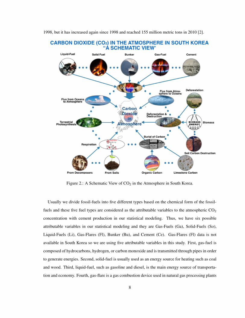
1998, but it has increased again since 1998 and reached 155 million metric tons in 2010 [2].
Figure 2.: A Schematic View of CO2 in the Atmosphere in South Korea.
Usually we divide fossil-fuels into five different types based on the chemical form of the fossil-
fuels and these five fuel types are considered as the attributable variables to the atmospheric CO2
concentration with cement production in our statistical modeling. Thus, we have six possible
attributable variables in our statistical modeling and they are Gas-Fuels (Ga), Solid-Fuels (So),
Liquid-Fuels (Li), Gas-Flares (Fl), Bunker (Bu), and Cement (Ce). Gas-Flares (Fl) data is not
available in South Korea so we are using five attributable variables in this study. First, gas-fuel is
composed of hydrocarbons, hydrogen, or carbon monoxide and is transmitted through pipes in order
to generate energies. Second, solid-fuel is usually used as an energy source for heating such as coal
and wood. Third, liquid-fuel, such as gasoline and diesel, is the main energy source of transporta-
tion and economy. Fourth, gas-flare is a gas combustion device used in natural gas processing plants
8

as well as oil or gas production sites having oil wells, gas wells, etc. Fifth, bunker is any type of oil
fuel used in ships. Lastly, we include cement as an attributable variable since a cement plant emits
CO2 during its process of production and most importantly the significant interactions of these risk
factors [18]. A schematic diagram of the attributable variables of CO2 emissions in the atmosphere
in South Korea in which data is available is given in Figure 2.
Tsokos and Xu (2013) analyzed carbon dioxide emission data for the United States and ranked the
attributable variables based on their percentage of contribution to atmospheric CO2 concentration
including all possible interactions among all six contributing variables. The number one contributor
to CO2 in the atmosphere is ‘liquid-fuel’, which contributes 17.59% of the total fossil-fuel CO2
emission. The second largest contributor to CO2 is ‘the interaction between liquid-fuel and cement’
with a 16.36% contribution rate. ‘The interaction between cement and bunker’ is ranked number
three with 15.73% contribution rate and ‘bunker’, ‘cement’, ‘gas-flare’, ‘gas-fuel’, ‘the interaction
between gas-fuel and gas-flare’, ‘the interaction between liquid-fuel and gas-flare’, and ‘the inter-
action between liquid-fuel and bunker’ are following next in the ranking [20].
Teodorescu, I and Tsokos, C (2013), have recently developed a data driven statistical model that
identified the attributable variables (risk factors) that contribute CO2 emissions in the European
Union (EU). The results are significantly different than those of the United States. The number
one contributor to CO2 is ‘gas-fuel’ with a 48.72% contribution rate followed by ‘the interaction
between gas-fuel and bunker-fuel’ with a 12.41% contribution rate. Six other variables and interac-
tions follow in the ranking of contributable variables to CO2 emissions [11].
In the present chapter we have yearly CO2 emissions data for each of the fossil-fuels in metric
tons for South Korea that was obtained from Carbon Dioxide Information Analysis Center (CDIAC)
from 1971 to 2008. Using the subject data we develop a statistical model that contains the signif-
icant contributable variables, as shown in the Schematic Diagram, Figure 2, along with important
interactions. These significantly contributing variables to CO2 emissions are ranked and compared
with those of the United States and European Union. The validation and quality of the proposed
statistical model has been established along with the usefulness of the developed model.
9
2.2 Materials and Methods
2.2.1 Data
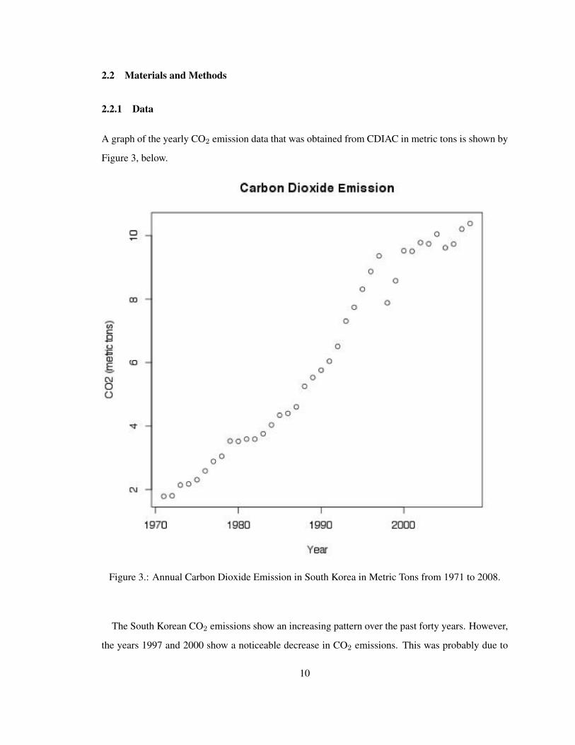
A graph of the yearly CO2 emission data that was obtained from CDIAC in metric tons is shown by
Figure 3, below.
Figure 3.: Annual Carbon Dioxide Emission in South Korea in Metric Tons from 1971 to 2008.
The South Korean CO2 emissions show an increasing pattern over the past forty years. However,
the years 1997 and 2000 show a noticeable decrease in CO2 emissions. This was probably due to
10

the economic crisis that South Korea was experiencing during this period.
2.2.2 Statistical Modeling
In developing the statistical model for CO2 emissions as a function of the attributable variables, we
require the data to follow the Gaussian probability distribution. We have shown through goodness-
of-fit testing that the subject data does not follow the normal probability distribution. The Q-Q plot
of the CO2 emission data, shown in Figure 4, supports this fact.
Figure 4.: Q-Q Plot for the Dependent Variable CO2.
11

To overcome this important assumption we applied the Johnson Transformation [4], to the data
and it transforms it to justify the basic assumption to proceed with developing the statistical model.
In the modeling process the CO2 emissions will be the response variable and Gas-Fuels (Ga),
Solid-Fuels (So), Liquid-Fuels (Li), Bunker-Fuels (Bu), and Cement (Ce) will be the attributable
variables along with the significantly contributing interactions. The theoretical form of the statistical
model is of the form given by
CO2 = ↵+
X
i
�ixi +X
j
�jtj + ✏ , (2.1)
where ↵ is the intercept of the model, �i is the coefficient of ith individual attributable variable
xi, �j is the coefficient of jth interactions term tj , and ✏ is the error term of the model.
Since the dependent variable CO2 emission does not follow the Gaussian probability distribution,
as we mentioned above, we shall apply the Johnson Transformation [4] to the subject data, which
results in the following equation.
TCO2 = �0.1653 + 0.4290 · log✓
CO2 � 1.7197
10.4122� CO2
◆, (2.2)
where TCO2 is the dependent variable after the Johnson transformation.
The transformed dependent variable TCO2 satisfies the normality condition and now we proceed
to build the statistical model with all five individual attributable variables and all possible interaction
terms among the individual attributable variables. The best statistical model with all significant in-
dividual variables and interactions that estimates almost all of the CO2 emissions in the atmosphere
in South Korea is given by
ˆTCO2 = �2.9435 + 0.9828⇥ 10
�4Li+ 1.0704⇥ 10
�4So
�0.0427⇥ 10
�4Ga� 8.1591⇥ 10
�4Bu
�4.2632⇥ 10
�9LI · So+ 8.4286⇥ 10
�9LI ·Ga
+7.0671⇥ 10
�9LI ·Bu+ 2.8014⇥ 10
�8So ·Bu
�4.3137⇥ 10
�8Ga ·Bu� 1.9501⇥ 10
�13Li · So ·Bu .
(2.3)
12

The TCO2 estimate obtained from equation (2.3) is based on the transformed version of the data.
Thus, we can estimate the actual CO2 emissions using the transformed version of equation (2.3),
that is,
ˆCO2 =�1.1698� 10.4122 · e2.331· ˆTCO2
�0.680237� e2.331· ˆTCO2. (2.4)
Thus, for a set of given values of the attributable variables we can use the proposed statistical
model to obtain estimates of the CO2 emissions in the atmosphere.
To attest to the quality of the proposed statistical model we use the coefficient of determination,
R2 and adjusted R2 criteria that attest to the fitting quality of the subject model. The regression sum
of squares (SSR), also referred to as the explained sum of squares, is the variation that is explained
by the proposed model. The sum of squared errors (SSE), also called the residual sum of squares, is
the variation that is left unexplained. The total sum of squares (SST) is proportional to the sample
variance and equals the sum of SSR and SSE. The coefficient of determination R2 is defined as the
proportion of the total response variation that is explained by the proposed model. It provides an
overall measure of how well the model fits the given data. Thus, R2 is given by
R2= 1� SSE
SST.
The R2 adjusted will adjust for degrees of freedom of the model and it is preferred when we are
working with several parameters and is given by
R2adj = 1� SSE/dferror
SST/dftotal.
For our proposed statistical model both R2 and R2 adjusted are approximately the same, 0.9941.
That is, the proposed statistical model explains 99.41% of the variation in the response variable, a
very high quality model. Equivalently, the attributable variables that we included in the model along
with the relevant interactions estimate 99% of the CO2 emissions in the atmosphere.
13

We also performed residual analysis, that is, the actual annual CO2 emission minus the model
estimate of CO2 emission. A plot of the results is given in Figure 5.
Figure 5.: Residual Plot.
The residual analysis also attests to the excellent quality of the developed model, where the mean
residual is very small, that is,
r̄ =
1
n
Xri = 6.8⇥ 10
�19 .
14

2.3 Results and Discussion
2.3.1 Ranking of the Contributing Variables - South Korea
We utilize the R2 criteria to rank the attributable variables along with the significant interactions
with respect to the percent of contribution of CO2 emissions in the atmosphere. Table 2 below
shows the rankings of these risk factors along with their percent of the overall contribution.
Table 2: The Rank of Attributing Variables (South Korea).
Rank Variables Contribution (%)
1 Liquid-Fuels (Li) 75.37
2 Solid-Fuels (So) 18.61
3 So & Bu 2.008
4 Ga & Bu 1.534
5 Li & Bu 0.912
6 Bunker-Fuels (Bu) 0.47
7 Gas-Fuels (Ga) 0.224
8 Li & So 0.207
9 Li & Ga 0.062
10 Li & So & Bu 0.004
The risk variable that has the biggest contribution to the CO2 emission in South Korea is Liquid-
Fuels, which contributes 75% of the CO2 emission. The next largest contribution is Solid-Fuels
with 18.61% of contribution. Note that numbers (rankings) 3, 4, and 5 are interactions of So & Bu,
Ga & Bu, and Li & Bu, respectively.
2.3.2 Ranking of the Contributing Variables - United States
Xu, Y and C. P. Tsokos [20] developed a data driven statistical model that identified the individual
attributable variables along with the significant interactions that contribute almost all the carbon
dioxide, CO2, emissions in the continental United States. These contributing entities are defined
and ranked along with the rate of contribution of CO2 in the atmosphere in Table 3 below.
Thus, these variables and interactions contribute 98.98% of CO2 emissions in the United States.
15

Table 3: The Rank of Attributing Variables (USA).
Rank Variables Contribution (%)
1 Liquid-Fuels (Li) 17.59
2 Li & Ce 16.36
3 Ce & Bu 15.73
4 Bunker-Fuels (Bu) 15.06
5 Cement (Ce) 10.77
6 Gas-Flares (Fl) 8.95
7 Gas-Fuels (Ga) 6.82
8 Ga & Fl 5.43
9 Li & Ga 2.25
10 Li & Bu 0.02
2.3.3 Ranking of the Contributing Variables - European Union
Recently, Teodorescu, I and C. P. Tsokos [11, 12] structured a nonlinear statistical model using CO2
emissions data for the European Union Countries (EU). They identified that Gas-Fuels contributes
48.72% of the overall CO2 emissions. The Table 4 below includes the other individual contributions
of CO2 emission along with the significant contributing interactions for EU.
Table 4: The Rank of Attributing Variables (EU).
Rank Variables Contribution (%)
1 Gas-Fuels (Ga) 48.72
2 Li & Bu 12.41
3 Li2 11.79
4 Bu2 7.78
5 Gas-Flares (Fl) 6.66
6 Li & Fl 5.06
7 Li & Bu 4.71
8 Liquid-Fuels (Li) 2.86
16

2.3.4 Comparison: U.S., EU, and South Korea
The Table 5 below gives an interesting comparison of what contributes to the CO2 emissions in the
atmosphere in the United States, European Union, and South Korea. There seems to be significant
non-uniformity among the three countries that we have studied.
Table 5: The Rank Comparison.
Rank USA S. Korea EU
1 Li Li Ga
2 Li & Ce So Li & Bu
3 Ce & Bu So & Bu Li2
4 Bu Ga & Bu Bu2
5 Ce Li & Bu Fl
6 Fl Bu Li & Fl
7 Ga Ga Li & Bu
8 Ga & Fl Li & So Li
9 Li & Ga Li & Ga -
10 Li & Bu Li & So & Bu -
Of significant importance is that 75% of the CO2 emissions in South Korea is caused by Liquid-
Fuels, whereas in the US this attributable variable contributes only 17%. The EU had almost 50%
of its CO2 emissions contributed by Gas-Fuels alone.
Furthermore, the number one attributable variable in the US and South Korea is Liquid-Fuels. It
is the last in EU with only 2.86% contribution to CO2 emissions.
It is also interesting to note that the US and South Korea had five significant contributing interac-
tions of the risk factors while EU had only three contributing to CO2 emissions. This information
is clearly displayed in Figure 6.
It is interesting to note that in South Korea “Li+So” contribute 94% of the CO2 emissions in the
atmosphere whereas “Li+Bu+Ce” contribute 76% in the United States and “Ga+Li+Bu” contribute
88% in the European Union countries.
17

Figure 6.: Top Attributing Variables by Country.
2.4 Conclusion / Contributions
We have developed a data driven statistical model that identifies the risk variables and their interac-
tions that cause the carbon dioxide emissions in the atmosphere in South Korea. South Korea ranks
eighth in the world in total CO2 emissions from fossil-fuels burning, cement production, and gas
flaring, with mainland China being the number one with 2,259 millions metric tons of CO2. We
have identified that almost all of the CO2 emissions in South Korea are caused by liquid-fuels (Li),
solid-fuels (So), bunker-fuels (Bu), and the interactions of So and Bu, Ga and Bu, and Li and Bu.
The developed model offers several significant uses in the subject area. First, for a given set
of the risk factors (attributable entities) you can obtain good estimates / predictions of the CO2
emissions in the atmosphere. Second, it can identify the important interactions of the contributing
entities. Third, it can rank the attributable variables as a function of the percent of contribution to
18

CO2 emissions in the atmosphere. Fourth, one can perform surface response analysis to identify
the amounts that each attributable variable should contribute so that you can control (minimize) the
CO2 emissions in the atmosphere. Lastly, we can calculate confidence limit with a desirable specific
degrees of confidence that will be useful in controlling the CO2 emissions.
The above information that can be obtained from the proposed statistical model is essential in
developing strategic polices to control CO2 emissions in the South Korean atmosphere.
In addition, we have compared the attributable variables of the CO2 emissions of South Korea
with those of the United States and European Union countries. Some of the interesting comparisons
are: Liquid-Fuels are the number one contributors to the CO2 emissions in South Korea and the
United States, whereas they are the least (last) contributors in the European Union, in South Korea
75.37% of the CO2 emissions are caused by Liquid-Fuels and only 17.59% in the United States
and only 2.86% in the European Union countries, and in the United States there are five significant
interactions of the attributable variables that contribute to the CO2 emissions, while there are six in
South Korea and only three in European Union countries.
19
Chapter 3
Transitional Modeling of the Carbon Dioxide in the Atmosphere by Climate Regions in the
United States
3.1 Introduction
One of the main issues in our planet is the climate change problem; rising atmospheric temperature,
the shifted patterns of snow and rainfall, and much more extreme climate changes are daily features
in our media. Scientists speak with confidence that all these problems are related to climbing levels
of the atmospheric carbon dioxide (CO2) emission along with other growing greenhouse gases such
as methane (CH4), nitrous oxide (N2O), and fluorinated gases in the atmosphere. These greenhouse
gases absorb the thermal radiation from the surface of the earth and radiate again to the surface, and
this repeating process elevates the atmospheric temperature.[25][26]
The CO2 in our atmosphere has increased dramatically after the industrial revolution (1760). The
risk of increasing CO2 emission is not only on the amount of the CO2 in the atmosphere but also on
the survival time of the CO2 in the atmosphere; it remains in our atmosphere for thousands of years.
Before the industrial revolution, the CO2 level never increased more than 30 ppm in any period;
however, it has increased more than 30 ppm within the past two decades alone. Also the proportion
of the CO2 among all greenhouse gases emission in the United States reached 82% in 2012, and
this speaks of the importance of controlling the CO2 emission and, in fact, we are able to reduce the
level of the CO2 emission by controlling related human activities.[27]
The world’s top polluter of CO2, China, pledged to peak the CO2 emissions around 2030 after a
remarkably rapid increase of the CO2 emission in the 21st century, whereas the world’s second CO2
polluter, the United States, already reached the peak prior to 2010 and promised to try to cut the
CO2 emission by at least 26% from 2005 levels by 2025.[28] In order for the United States to carry
out this promise, more efficient regulations must be established. The present study provides a rough
sketch of the CO2 problem in the US and recommends that regional policies based on our findings
20

will be more effective. Also, additional interesting research on the subject area can be found in the
references,[5], [9], [10], [11], [12], [13], [14], [15], [16], [17], [19], and [20].
3.2 Statistical Modeling
3.2.1 The Data
Figure 7.: Structure of Data with Sample Size in Each Level.
The original data used in the present study is obtained from the United States Environmental
Protection Agency (EPA) and contains state CO2 emission inventories from fossil fuel combustion
by end-use sectors; the commercial, electric power, industrial, residential, and transportation sector,
in million metric tons of CO2 from 1992 through 2012 for all 50 states in the United States. The
structure of the data with sample size in each level is displayed in Figure 7.
Figure 8 shows the the data structure based on 9 US climate regions with 5 end-use sectors, and
the following data modification enables us to perform a transitional modeling of the data.
Iij =
8><
>:
0, if ryij ryj
1, otherwiseand Skij =
8><
>:
0, if rxkij rxkj
1, otherwise,
21

where i(= 1, 2, ..., 51) is a state index, j(= 1993, 1994, ..., 2012) is a year index, k(= 1, 2, ..., 5)
is a sector index (1: commercial sector, 2: electric power sector, 3: industrial sector, 4: residential
sector, 5: transportation sector), yij is the CO2 emission for the state i in year j, ryij =
yij�yi,j�1
yi,j�1
for all i and j, xkij is the CO2 emission due to the sector k for the state i in year j, and rxkij =
xkij�xki,j�1
xki,j�1for all j in each k.
Figure 8.: Illustration of US Climate Regions with CO2 Emission Sectors.
3.2.2 Transitional Modeling
The key idea of the present study is predicting the probability that the changing rate of the CO2
emission in a specific region is higher than the average changing rate based on values of attributable
variables in the past over all climate regions. While we use the past response values as independent
variables in direct transitions for the ordinary transitional modeling[29][30], the indirect transition
method has been applied in the present study. In other words, our interest in this modeling procedure
22

is on the statistical modeling of
Pr(Iij = 1 | Sk i j�1 , where k = 1, 2, ..., 5.).
The equation (3.1) below represents the theoretical indirect transition model of the regional data,
and equation (3.2) shows the fitted probability models for all 9 US climate regions along with the
table of the estimated coefficients.
logit(E[Iij ]) = �0 +9X
r=1
"�r(tij · gir) +
5X
k=1
�9k+r(Sk i j�1 · gir)#, (3.1)
where r is a categorical variable indicating below regions:
r 1 2 3 4 5 6 7 8 9
Region C ENC NE NW S SE SW W WNC
,and where tij = j � 1990 for all 50 states, and gir = 1, if state i belongs to region r, gir = 0,
otherwise.
⇡̂r =exp( ˆ�0 + ˆ�1tij +
P5k=1
ˆ�k+1Sk i j�1)
1 + exp( ˆ�0 + ˆ�1tij +P5
k=1ˆ�k+1Sk i j�1)
(3.2)
Table 6: Estimated Coefficients in the Equations (3.2).
Region ˆ�0 ˆ�1 ˆ�2 ˆ�3 ˆ�4 ˆ�5 ˆ�6
C -0.3848 0.0317 0.1005 -0.9000 0.6631 -0.2748 0.5202
ENC -0.3848 0.0774 -0.5266 -1.8590 0.3162 1.6961 -0.5375
NE -0.3848 0.0593 0.1332 -1.2377 0.4604 1.0280 0.0271
NW -0.3848 0.0092 -0.3751 -0.3450 0.6133 0.4202 -0.4589
S -0.3848 0.0199 -0.2813 -0.4035 0.9975 -0.4903 -0.5316
SE -0.3848 0.0421 -0.5519 -0.9326 0.2614 0.2175 0.2121
SW -0.3848 -0.0296 -0.3225 -0.6208 0.3235 1.0365 -0.3863
W -0.3848 0.0361 -0.5263 -0.5422 -0.4334 0.5534 0.5709
WNC -0.3848 -0.0326 0.2560 1.3760 -0.2732 -0.4342 -0.0973
23

Probabilities that the CO2 emission in each region is more than the average US CO2 emission at
tij based on all possible combinations of Sk i j�1, k = 1, 2, 3, 4, 5, are displayed in Table 7. For
example,
1� Pr(Iij = 1 | S1 i j�1 = S3 i j�1 = S5 i j�1 = 1) = 0.8359
, and
2� Pr(Iij = 1 | S3 i j�1 = S5 i j�1 = 1) = 0.8217
in the central region, and this implies that the contributions of the sector 3 and the sector 5 to the
regional CO2 emissions are statistically significant in the central region. Accordingly, the main key
factors causing CO2 emission in the central region are the industrial sector and the transportation
sector. Although the sector 1, the commercial sector, also contributes to the highest probability, the
marginal contribution to the highest probability is only 0.0142 (0.8359 � 0.8217) and it is not as
significant as two other sectors; the industrial and transportation sector. When we look into the east
north central region, the contribution of the sector 4, the residential sector, to the atmospheric CO2
emission in this region is remarkably obvious while the sector 3, the industrial sector, has merely
small effects on the CO2 emission compare to the residential sector, because
Pr(Iij = 1 | S3 i j�1 = S4 i j�1 = 1) = 0.9679
and
Pr(Iij = 1 | S4 i j�1 = 1) = 0.9565
with 0.0114 (0.9679� 0.9565) as a marginal contribution of the industrial sector.
Table 7: Probabilities for All Possible Cases.
S1 S2 S3 S4 S5 C ENC NE NW S SE SW W WNC
0 0 0 0 0 0.5852 0.8015 0.7269 0.4568 0.5182 0.6419 0.2562 0.6096 0.2433
1 0 0 0 0 0.6094 0.7045 0.7526 0.3663 0.4481 0.5079 0.1997 0.4798 0.2935
0 1 0 0 0 0.3645 0.3861 0.4357 0.3733 0.4181 0.4136 0.1562 0.4758 0.5601
0 0 1 0 0 0.7325 0.8470 0.8084 0.6083 0.7447 0.6995 0.3225 0.5030 0.1966
0 0 0 1 0 0.5174 0.9565 0.8815 0.5614 0.3971 0.6902 0.4927 0.7308 0.1724
0 0 0 0 1 0.7036 0.7022 0.7323 0.3470 0.3873 0.6890 0.1897 0.7343 0.2258
1 1 0 0 0 0.3881 0.2709 0.4687 0.2904 0.3516 0.2888 0.1183 0.3491 0.6218
1 0 1 0 0 0.7517 0.7658 0.8282 0.5162 0.6876 0.5727 0.2564 0.3742 0.2402
1 0 0 1 0 0.5424 0.9286 0.8948 0.4680 0.3321 0.5620 0.4130 0.6160 0.2120
1 0 0 0 1 0.7241 0.5821 0.7576 0.2675 0.3230 0.5606 0.1450 0.6201 0.2737
0 1 1 0 0 0.5268 0.4632 0.5503 0.5238 0.6608 0.4781 0.2038 0.3705 0.4921
0 1 0 1 0 0.3035 0.7743 0.6834 0.4755 0.3056 0.4671 0.3430 0.6122 0.4519
0 1 0 0 1 0.4911 0.2687 0.4424 0.2735 0.2969 0.4658 0.1118 0.6164 0.5360
0 0 1 1 0 0.6754 0.9679 0.9218 0.7027 0.6411 0.7431 0.5731 0.6377 0.1368
24

Table 7: Probabilities for All Possible Cases.
S1 S2 S3 S4 S5 C ENC NE NW S SE SW W WNC
0 0 1 0 1 0.8217 0.7639 0.8125 0.4953 0.6315 0.7421 0.2445 0.6418 0.1817
0 0 0 1 1 0.6433 0.9278 0.8843 0.4472 0.2791 0.7336 0.3976 0.8278 0.1589
1 1 1 0 0 0.5518 0.3376 0.5830 0.4305 0.5952 0.3453 0.1564 0.2580 0.5558
1 1 0 1 0 0.3252 0.6695 0.7115 0.3839 0.2493 0.3355 0.2744 0.4826 0.5158
1 1 0 0 1 0.5162 0.1783 0.4754 0.2055 0.2417 0.3343 0.0835 0.4870 0.5987
1 0 1 1 0 0.6970 0.9469 0.9309 0.6190 0.5741 0.6249 0.4930 0.5098 0.1699
1 0 1 0 1 0.8359 0.6564 0.8320 0.4028 0.5640 0.6237 0.1899 0.5142 0.2229
1 0 0 1 1 0.6660 0.8836 0.8973 0.3573 0.2261 0.6133 0.3235 0.7395 0.1962
0 1 1 1 0 0.4582 0.8247 0.7738 0.6260 0.5440 0.5324 0.4191 0.5058 0.3856
0 1 1 0 1 0.6519 0.3352 0.5570 0.4100 0.5338 0.5311 0.1481 0.5102 0.4678
0 1 0 1 1 0.4230 0.6671 0.6892 0.3643 0.2055 0.5201 0.2619 0.7365 0.4280
0 0 1 1 1 0.7778 0.9464 0.9238 0.5990 0.5121 0.7815 0.4770 0.7570 0.1257
1 1 1 1 0 0.4833 0.7354 0.7962 0.5350 0.4738 0.3960 0.3432 0.3768 0.4477
1 1 1 0 1 0.6744 0.2294 0.5895 0.3232 0.4636 0.3947 0.1119 0.3810 0.5317
1 1 0 1 1 0.4477 0.5420 0.7170 0.2825 0.1633 0.3843 0.2045 0.6228 0.4915
1 0 1 1 1 0.7947 0.9124 0.9326 0.5066 0.4421 0.6732 0.3979 0.6480 0.1567
0 1 1 1 1 0.5873 0.7333 0.7785 0.5141 0.4122 0.5847 0.3290 0.6443 0.3628
1 1 1 1 1 0.6114 0.6188 0.8006 0.4210 0.3461 0.4477 0.2621 0.5170 0.4238
3.3 Cluster Analysis
We develop six cluster-maps showing the atmospheric CO2 emission regions in the United States
based on effects of the total CO2 emission and all five end-use sectors; the commercial, electric
power, industrial, residential, and transportation sector. After normalizing the probability data in
Table 7 using Johnson’s transformation, [31] and [32], the hierarchical clustering procedure has
been performed using Ward’s method, in which we consider a clustering problem as a problem of
minimizing within-cluster sum of squares in each cluster rather than a distance problem[33][34][35].
In Ward’s method, we begin with 9 clusters of size 1 and combine two clusters that render the min-
imum error sum of squares in equation (3.3), or yield maximum R2 in equation (3.4) equivalently,
repeating this procedure until we reach the optimal R2 value with the number of clusters we desired.
1� SSE =
X
l
X
r
X
m
�Plrm � ¯Pl·m
�2, (3.3)
2� R2=
SST � SSE
SST, (3.4)
, and
25
(Continued)

3� SST =
X
l
X
r
X
m
�Plrm � ¯P··m
�2, (3.5)
where Plrm denotes the probability after Johnson’s transformation for the mth combination of
Sk i j�1 (k = 1, 2, 3, 4, 5) in region r belonging to the cluster l.
Table 8 illustrates the results of the hierarchical clustering using Ward’s method based on effects
of total CO2 emission, the commercial, electric power, industrial, residential, and transportation
sector denoted by Total, S1, S2, S3, S4, S5, respectively along with R2 values for all clustering
criteria.
Table 8: Clustering Based on Different Factors.
RegionClustering Based on
Total S1 S2 S3 S4 S5
C C 1 C 1 C 2 C 2 C 2 C 2
ENC C 2 C 2 C 2 C 1 C 3 C 3
NE C 2 C 1 C 2 C 1 C 1 C 1
NW C 1 C 2 C 1 C 2 C 1 C 3
S C 1 C 2 C 1 C 2 C 2 C 3
SE C 1 C 3 C 2 C 1 C 1 C 1
SW C 3 C 2 C 1 C 1 C 3 C 3
W C 1 C 3 C 1 C 3 C 1 C 2
WNC C 3 C 1 C 3 C 3 C 2 C 1
R2 0.566 0.869 0.838 0.898 0.853 0.822
3.3.1 Clustering Based on the Effect of the Total CO2 Emissions
In Figure 9, we see that nine US climate regions are combined into three CO2 emission clusters
based on the effect of the total CO2 emission.
The cluster 1 consists of five US climate regions; the central, northwest, south, southeast, and west
regions, and the cluster 2 is composed of the east north central and northeast regions. Finally the
remaining two regions; the west north central and southwest regions, build the cluster 3. Regions
26
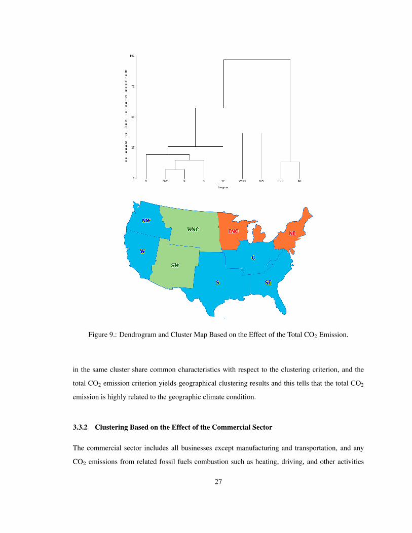
Figure 9.: Dendrogram and Cluster Map Based on the Effect of the Total CO2 Emission.
in the same cluster share common characteristics with respect to the clustering criterion, and the
total CO2 emission criterion yields geographical clustering results and this tells that the total CO2
emission is highly related to the geographic climate condition.
3.3.2 Clustering Based on the Effect of the Commercial Sector
The commercial sector includes all businesses except manufacturing and transportation, and any
CO2 emissions from related fossil fuels combustion such as heating, driving, and other activities
27
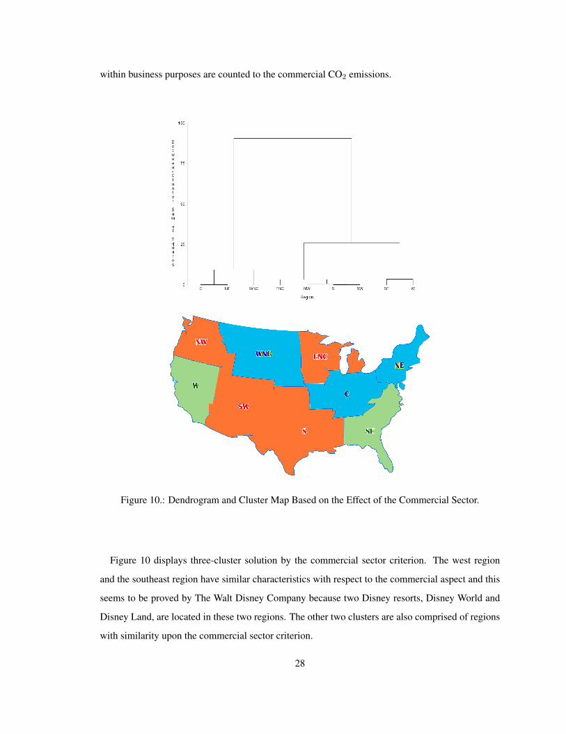
within business purposes are counted to the commercial CO2 emissions.
Figure 10.: Dendrogram and Cluster Map Based on the Effect of the Commercial Sector.
Figure 10 displays three-cluster solution by the commercial sector criterion. The west region
and the southeast region have similar characteristics with respect to the commercial aspect and this
seems to be proved by The Walt Disney Company because two Disney resorts, Disney World and
Disney Land, are located in these two regions. The other two clusters are also comprised of regions
with similarity upon the commercial sector criterion.
28

3.3.3 Clustering Based on the Effect of the Electric Power Sector
Figure 11.: Dendrogram and Cluster Map Based on the Effect of the Electric Power Sector.
The electric power sector not only involves the generation of the electricity but also includes
transmission and distribution of the electricity. The CO2 emission from the electric power sector
makes up about 32% of the total amount of CO2 emission in the United States and this is the top
contributing sector among all five sectors to the CO2 emission in the United States.
The electric power sector criterion also highlights three-cluster solution with reasonably well
combined cluster map in Figure 11. The relationship between the electric power sector and the CO2
29

emission can be found in the source of the electric power and the amount of the electric usage. The
geographical distribution of the type of the major power plants in Figure 12 proves such a rela-
tionship. Most of the steam and nuclear power plants are located in the cluster with the southeast,
central, east north central, and northeast regions, whereas we find major hydroelectric power plants
in the cluster with the northwest, west, southwest, and south regions.
Figure 12.: A Breakdown of the Major Power Plants in the United States, by Type.
3.3.4 Clustering Based on the Effect of the Industrial Sector
The industrial sector emits the CO2 directly and indirectly to our atmosphere. The direct way of
emissions involves burning fossil fuels to produce commercial goods, and the CO2 emission at a
power plant to generate electricity to use in industrial facilities is categorized to the indirect way of
emissions. The industrial sector occupies around 20% of total CO2 emissions in the United States.
Figure 13 shows similarities between the west and west north central regions, among the north-
west, south, and central regions, and among the other four regions. In order to control the CO2
emission from the industrial aspect in each cluster, we need further scientific research, which may
suggest re-location of chemical plants that may have significant interaction effects, as a solution of
reducing CO2 emission nationwide.
30

Figure 13.: Dendrogram and Cluster Map Based on the Effect of the Industrial Sector.
3.3.5 Clustering Based on the Effect of the Residential Sector
The residential sector increases the atmospheric CO2 concentration through heating, cooking, and
other home maintaining activities. Although the contribution of the residential sector to the total
CO2 emission is less than 10% in the United States, it is very important to control the emission due
to the residential sector because every individual is a member of this residential sector and the effect
of a campaign against the CO2 emission may reach all other sectors.
Clustering based on the residential sector criterion also provides three-cluster solution in Figure
31

Figure 14.: Dendrogram and Cluster Map Based on the Effect of the Residential Sector.
14. One remarkable feature of this clustering is that the cluster, comprised of the northwest, west,
northeast, and southeast regions, includes all the Pacific and Atlantic seaside regions, while other in-
land regions form the other two clusters. It is very interesting that the effect of the residential aspect
to the CO2 emission is related to the human lifestyle founded on the geographic characteristics.
32

Figure 15.: Dendrogram and Cluster Map based on the Effect of the Transportation Sector.
3.3.6 Clustering Based on the Effect of the Transportation Sector
The transportation sector produces the atmospheric CO2 through the movement of merchandise and
people by the combustion of petroleum-based products such as gasoline, diesel, and bunker fuels.
This sector has the second greatest contribution to the total CO2 emissions, about 28%, in the United
States.
Figure 15 shows similarities between the west and central regions, among the southeast, north-
east, and west north central regions, and all remaining regions. This three-cluster solution provides
33

reasonable evidence to share regulations to reduce the CO2 emission in a transportation aspect for
regions within the same cluster.
3.4 Conclusion / Contributions
The present study provides several guidelines, for policy makers, to effectively control the level of
the carbon dioxide emissions in each US climate region. Firstly, fitted regional probability models
driven by equation (3.2), derived from transitional models in equation (3.1), that allow us to calculate
the probabilities of the CO2 emission at risk in each region based on all possible combinations of
by-sector CO2 emission behaviors in the previous year. Ranks of the effect of by-sector behaviors
to the level of the CO2 emissions in each climate region are displayed in Table 9, below.
Table 9: Ranks of Sectors with Maximum Probabilities in Each Region.
RegionRanks with Maximum Probability
Rank 1 Rank 2 Rank 3 Max. Prob.
C S3 S5 S1 0.8359
ENC S4 S3 S1 0.9679
NE S4 S3 S1 0.9326
NW S3 S4 S2 0.7027
S S3 S1 S2 0.7447
SE S3 S4 S5 0.7815
SW S4 S3 S1 0.5731
W S5 S4 S3 0.8278
WNC S2 S1 S5 0.6218
We can conclude that the number one risk sector in the central region is S3, the industrial sec-
tor, the number two risk sector is S5, the transportation sector, and the rank three sector is S1, the
commercial sector. Accordingly, the industrial sector CO2 emission has a role of a preceding in-
dex when we predict how the CO2 emission changes in the following year for the central region.
Similarly, we consider the residential sector CO2 emission as a preceding index for the east north
central region, the transportation sector CO2 emission as a leading index for the west region, and
34

so on. Moreover, ranks in Table 9 are assigned under consideration of interaction effects among all
possible combinations of five sectors. Secondly, we can effectively control the total CO2 emission
using CO2 clusters by the effect of each sector shown in Table 8. For instance, we may apply the
same policy regarding the residential sector to all west and east coastal regions because they share
similar properties within residential related problems as shown in Figure 14.
Providing a solution to an environmental problem is not so simple because most environmental
problems are due to human activities that are not predictable. However, these statistical models
would be a strong background for our government to legislate more effective regulations to control
the optimal level of the CO2 emission in the United States on regional basis.
35

Chapter 4
Active and Dynamic Approaches for Clustering Time Dependent Information
4.1 Introduction
We are living in the world with a flood of information which changes over time, and this time depen-
dent information occupies the main part of BIG DATA that is the current prime topic in data science.
There have been several statistical approaches [36][37][38][44][45][46][47][48][49][50][51] to ex-
tract the significant core from time dependent information, and in the present study, we propose
new methods to obtain the important essence from the time dependent information by clustering
time dependent responses such as time series data and longitudinal data we are commonly faced
with to analyze. Figure 16, below describes time dependent information we deal with in Statistics
and we focus on time series data and a part of longitudinal data in the present study.
Classical methods in clustering time dependent information were a sort of a passive approach
from a data scientist’s viewpoint, because resulting clusters followed by these methods are deter-
ministic based on the measure of dissimilarity no matter what distance measurements we applied to
the data. However, the new methods we are proposing in the present study are active processes to
deliver the core information from the massive information we are facing to be analyzed based on
our objective of the present study.
In general, we have three different clustering approaches for time dependent information as shown
in Figure 16, that is,
1� Temporal-Proximity-Based Clustering Approach.
2� Representation-Based Clustering Approach.
3� Model-Based Clustering Approach.
Our proposed methods are developed in order to accommodate and improve problems inherited from
imposing several assumptions in temporal-proximity-based clustering approach. In temporal-
36

Figure 16.: Summary of Time Dependent Information in Statistics.
proximity-based approach, we assume that there is plenty of information available in each time
series object, and only one stream of information is given as a function of time.
But, what if we do not have enough number of observations to use classical time series clus-
tering methods, and what if there exist several significant streams of information in each time
series object? Thus, we proceed to introduce two new clustering methods to cover these important
cases in temporal-proximity-based approach. Moreover, those classical time series clustering
methods do not count actual time dependencies among time series objects and the resulting clusters
are usually based on trends and patterns. Hence, we are not able to investigate their actual degree
of time dependencies if we use classical time series clustering methods.
4.2 Motivation
In what follows we discuss the new methods we propose.
4.2.1 Lag Target Time Series Clustering
The first approach we propose in the current study is “Lag Target Time Series Clustering (LTTC)”.
In time series analysis, we usually consider more than 50 observations in each time series objects
37

(responses) as possibly enough information, but this condition is not always satisfied in the real
world problem. However, if we take cross lag distances into consideration, we can increase the
number of distance measurements considerably.
Figure 17.: Illustration of the Importance of the Cross Lag Distance.
In Figure 17, below, Xt is the baseline time series object, Yt is a vertical shifted time series object
of Xt, and Zt is a preceding index of Xt. Now, which information is more closely related to
the baseline time series object, Xt? If we ignore lag-time-dependency between two time series
objects, we have
d(Xt, Yt) <<< d(Xt, Zt) ,
no matter what distance measure method we use. However, if we measure cross lag-one distance
between two time series objects, we obtain
38

d(Xt�1, Yt) >>> d(Xt�1, Zt) .
Now, suppose we have two different clusters, one with Yt and the other with Zt, then, does Xt
go with the cluster with Yt? or Zt? We definitely need to include all three time series objects in
the same cluster and we will be able to obtain this desirable resulting cluster using our proposed
method, LTTC.
4.2.2 Multi-Factor Time Series Clustering
The second method we propose in the present study is “Multi-Factor Time Series Clustering
(MFTC)”. This method (MFTC) is more meaningful as a more realistic approach to our previously
proposed method, LTTC. As we already mentioned in the introduction, one of the general assump-
tions in classical temporal-proximity-based time series clustering is that there exists only one stream
of information in each time series objects. However, usually each time series response consists of
several sub-information. For example, daily stock price consists of several sub-information such
as opening price, closing price, maximum price, and minimum price, etc. If each sub-information
shows different behavior and has a significant impact on the original information, we should take
these differences in consideration (sub-information) into our modeling. Also, in health science, sur-
vival analysis of patients is a function of time and death is caused by several factors, for example
in lung cancer, death was due to smoking, overweight, age, drinking, etc. Thus, we must take these
risk factors into consideration in modeling survival analysis. Therefore, when we measure the dis-
tance between two time series objects, we now put our ruler in the multi-dimensional space and the
degree of dimension is always “the number of factors considered in the study plus one”, because
of the time factor. If we just measure cross lag zero distance, it is very trivial as shown in Figure 18.
However, when we measure cross lag distances as shown in Figure 19, we have to consider the unit
difference between time and other factors and a weight factor which presented in the later section
replaces time unit.
39

Figure 18.: Two-Factor Distance Measurement at the Cross Lag zero.
Figure 19.: Two-Factor Distance Measurement at the Cross Lag One.
40

4.3 An Application of LTTC and MFTC: Brain Cancer Mortality Rates in the United States
In what follows we will apply our methods in some important real data.
4.3.1 Objective of the Study
There have been various mortality rates statistical models of brain cancer for the entire United States,
[39], [40], and [41]. However, we do not have any study done for various regional differences of
the brain cancer mortality rates in the United States. We strongly believe that there are significant
regional differences, primarily due to environmental issues such as carbon dioxide emission, the
quality of drinking water, etc. that cause death of brain cancer. Thus, our proposed method of
analytic clustering procedure based on regional brain cancer mortality rates in the United States is
very important.
4.3.2 Structure of the Data
Figure 20.: Structure of the Data.
The data that we are using was collected by the Surveillance, Epidemiology, and End Results
(SEER) database which is one of the biggest epidemiological databases in the U.S. and contain
U.S. state level mortality rates due to brain cancer from 1969 to 2012. Figure 20, above, shows the
structure of the data, with 9 climate regions, 51 states including D.C., and calculated mortality rates
for males and females separately. In each state, mt and ft represent the the number of deaths per
41

100,000 population due to brain cancer at time t(= 1, 2, ..., 43) for males and females, respectively.
Table 10, below, displays p-values from nonparametric Kruskal-Wallis tests for the hypothesis
that the median level of the brain cancer mortality rates of male and female are same in each state
of the United States, and calculated p-values in Table 10 suggest for us to consider MFTC method
to achieve the objective of the study.[42][52][53] For example, the largest p-value we have found
in Table 10 is 0.034 for the state of North Dakota and still this p-value is reasonably small enough
to decide that the differences between male brain cancer mortality rates and female brain cancer
mortality rates are statistically significant, when we set the level of significance, ↵, at 0.05.
Table 10: Comparison Between Male and Female Brain Cancer Mortality Rates.
State p-value State p-value State p-value
IL 1.56E-14 NH 6.40E-06 FL 4.85E-14
IN 1.30E-09 NJ 9.38E-14 GA 4.42E-13
KY 1.83E-08 NY 1.73E-15 NC 9.19E-08
MO 6.05E-11 PA 2.60E-08 SC 1.36E-08
OH 6.45E-15 RI 1.32E-05 VA 3.01E-11
TN 7.21E-12 VT 2.10E-05 AZ 7.56E-10
WV 1.94E-04 AK 6.78E-03 CO 5.40E-09
IA 2.14E-07 ID 2.27E-05 NM 4.92E-08
MI 3.59E-11 OR 7.62E-11 UT 3.74E-06
MN 2.82E-13 WA 7.21E-14 CA 1.41E-15
WI 6.79E-12 AR 5.21E-06 HI 4.48E-05
CT 1.24E-11 KS 1.60E-10 NV 3.56E-09
DE 7.92E-04 LA 7.97E-08 MT 3.10E-07
DC 7.14E-03 MS 1.28E-04 NE 1.34E-07
ME 5.58E-07 OK 3.70E-10 ND 3.40E-02
MD 2.24E-10 TX 7.62E-11 SD 6.78E-03
MA 6.79E-11 AL 2.65E-10 WY 7.32E-03
42

4.4 Construction of the Dissimilarity Matrix
Statistical clustering procedures are performed based on the dissimilarity matrix, which is a set
of pairwise distances among time series responses. Based on the structure of the data as shown
by Figure 20 and using the proposed method MFTC as presented in Table 10, we define pairwise
distances as follows.
4.4.1 Distance at the Cross Lag Zero
First, we define pairwise distances among mortality rates in all U.S. at the cross lag zero. Let
Ri =
2
6666664
mi1 fi1
mi2 fi2...
...
miT fiT
3
7777775
and
Rj =
2
6666664
mj1 fj1
mj2 fj2...
...
mjT fjT
3
7777775
be the brain cancer mortality rates in state i and state j, respectively, and define a difference matrix,
D = Ri �Rj =
2
6666664
mi1 �mj1 fi1 � fj1
mi2 �mj2 fi2 � fj2...
...
miT �mjT fiT � fjT
3
7777775
=
2
6666664
dm1 df1
dm2 df2...
...
dmT dfT
3
7777775.
43

Then the distance between state i and state j at cross lag zero is given by
dij =TX
t=1
qDtS�1D
0t ·Wt , (4.1)
where Dt is tth row of the difference matrix D, S is COV (Dm, Df ), and Wt is a weight factor,
which is the ratio of the absolute value of the sample autocorrelation, and is defined as,
Wt =
12T (|M |+ |F |)
PTt=1(|M |+ |F |)
,
where
M =
tX
⌧=1
(dm,⌧+T�t � ¯dm)(dm,⌧ � ¯dm)
and
F =
tX
⌧=1
(df,⌧+T�t � ¯df )(df,⌧ � ¯df ).
Equation (4.1) is basically a weighted Mahalanobis distance, and our distance measures are built
upon the Mahalanobis distance because the inverse covariance factor stabilizes the overall distance
matrix, thus, the effect of the weight factor is minimized and not over-counted, [43] [54] [55].
4.4.2 Distance at the Cross Lag k (k � 1)
We now define kRi, the brain cancer mortality rates in state i after eliminating k rows from the
front, and Rj,k, the brain cancer mortality rates in state j after removing k rows from the tail.
kRi =
2
6666664
mi,k+1 fi,k+1
mi,k+2 fi,k+2
......
mi,T fi,T
3
7777775
44
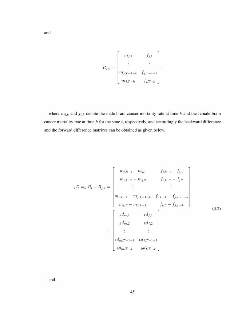
and
Rj,k =
2
6666664
mj,1 fj,1...
...
mj,T�1�k fj,T�1�k
mj,T�k fj,T�k
3
7777775,
where mi,k and fi,k denote the male brain cancer mortality rate at time k and the female brain
cancer mortality rate at time k for the state i, respectively, and accordingly the backward difference
and the forward difference matrices can be obtained as given below.
kD =k Ri �Rj,k =
2
6666666664
mi,k+1 �mj,1 fi,k+1 � fj,1
mi,k+2 �mj,2 fi,k+2 � fj,2...
...
mi,T�1 �mj,T�1�k fi,T�1 � fj,T�1�k
mi,T �mj,T�k fi,T � fj,T�k
3
7777777775
=
2
6666666664
kdm,1 kdf,1
kdm,2 kdf,2...
...
kdm,T�1�k kdf,T�1�k
kdm,T�k kdf,T�k
3
7777777775
(4.2)
and
45

Dk = Ri,k �k Rj =
2
6666666664
mi,1 �mj,k+1 fi,1 � fj,k+1
mi,2 �mj,k+2 fi,2 � fj,k+2
......
mi,T�1�k �mj,T�1 fi,T�1�k � fj,T�1
mi,T�k �mj,T fi,T�k � fj,T
3
7777777775
=
2
6666666664
dm,k,1 df,k,1
dm,k,2 df,k,2...
...
dm,k,T�1�k df,k,T�1�k
dm,k,T�k df,k,T�k
3
7777777775
(4.3)
Based on equation (4.2) and (4.3), we can establish the cross lag k distance between state i and
state j as a mean of weighted backward Mahalanobis distance and weighted forward Mahalanobis
distance as given by the equation (4.4), below.
dij,k =
1
2
(
T�kX
t=1
qkDt kS�1
kD0t ·k Wt +
T�kX
t=1
qDt,k S
�1k D
0t,k ·Wt,k), (4.4)
where two weight factors, kWt and Wt,k, are defined below for k = 0, 1, 2, ..., T � 3.
kWt =
12(T�k)(|M1|+ |F1|)PT�k
t=1 (|M1|+ |F1|),
where
M1 =
tX
⌧=1
(kdm,⌧+T�k�t �k¯dm)(kdm,⌧ �k
¯dm)
and
F1 =
tX
⌧=1
(kdf,⌧+T�k�t �k¯df )(kdf,⌧ �k
¯df ),
and
Wt,k =
12(T�k)(|M2|+ |F2|)PT�k
t=1 (|M2|+ |F2|),
46

where
M2 =
tX
⌧=1
(dm,k,⌧+T�k�t � ¯dm,k)(dm,k,⌧ � ¯dm,k)
and
F2 =
tX
⌧=1
(df,k,⌧+T�k�t � ¯df,k)(df,k,⌧ � ¯df,k).
4.4.3 The Dissimilarity Matrix for Clustering
Using the distances we have defined above, we proceed to obtain l layers of the distance matrices
as shown in Figure 21, below. In each cross lag distance matrix in Figure 21, dij,k represents the
weighted mahalanobis distance between state i and state j at cross lag k.
Figure 21.: Structure of Distance Matrices.
In order to complete our final dissimilarity matrix for the clustering procedure, we define a weight
factor for each layer, which is the ratio of the absolute value of the sample cross-correlation as shown
by equation (4.5), and the resulting structure of the weight matrices as displayed in Figure 22. These
weight factors take the difference between genders and time dependency between two objects into
consideration at the same time properly. That is,
47

Figure 22.: Structure of Weight Matrices.
�ij,k =
12T (|M3|+ |F3|)
PT�3k=0 (|M3|+ |F3|)
(4.5)
where
M3 =
T�kX
⌧=1
(mi,⌧+k � m̄i)(mj,⌧ � m̄j)
and
F3 =
T�kX
⌧=1
(fi,⌧+k � ¯fi)(fi,⌧ � ¯fj).
In each layer in Figure 22, �ij,k denotes the weight for dij,k in Figure 21, that is the weight factor
applying to the distance between state i and state j at cross lag k.
Now, we proceed to multiply the distance layers in Figure 21 with the weight layers in Figure
22, and add all the resulting layers to build our final dissimilarity matrix presented in Figure 23 to
perform the statistical clustering procedure. At this stage, our main interest lies on the selection of
48

the optimal level of lag distance, and our final dissimilarity matrix is very sensitive to the choice of
the optimal level of lag, k.
Figure 23.: Final Dissimilarity Matrix.
In Figure 23, dij is the final similarity or dissimilarity index between state i and state j. In other
words, the sum of weighted cross lag distances between state i and state j.
4.5 Clustering Procedure
We utilize Ward’s Clustering Method in this section to achieve our resulting clusters. Joe H. Ward,
Jr.,[35][56][57], proposed a general agglomerative hierarchical clustering procedure which is based
on minimum variance criterion and it is also called ”Ward’s Minimum Variance Method”. In other
words, our final clusters are obtained by minimizing within-cluster variance which is defined by the
squared Euclidean distances among clustering objects as shown in equation (4.6), below.
dij = d({Xi}, {Xj}) = kXi �Xjk2 . (4.6)
4.5.1 Clusters Based on Euclidean Distance vs. Mahalanobis Distance
Before we move into our main clustering problem of the brain cancer mortality rates in the U.S.,
we want to compare the clustering results between Euclidean distance and Mahalanobis distance.
49

Figure 24, presents clustering maps based on Euclidean distance and Mahalanobis distance with the
same weight factors described in previous sections. We have four-cluster solution in both clustering
maps, and they are almost identical. Only two states stay in different clusters in both maps, and they
are Washington state and New Hampshire state. This implies that the covariance between males
and females are not significantly large, but this is still statistically significant because the covariance
stabilizes the pairwise distances so that we have appropriate level of the effect from using weight
factors.
4.5.2 Passive Deterministic Clustering vs. Active Dynamic Clustering
The map on the right side in Figure 24 delivers the resulting clusters based on our definition of
distances from equation (4.1). States in the green cluster are mostly located in the south region of
the U.S., and other colored clusters are also determined by the dissimilarity matrix with lag zero
which we obtained from the previous sections. With this approach, once we have a dissimilarity
matrix where the clustering solution is only determined by the clustering method we want to choose.
We refer to this classical approach as “Passive Deterministic Clustering” in this sense.
The algorithm of LTTC is presented in Figure 25, and this procedure is an active and dynamic
way to cluster time series responses, because the final cluster solution is the end objective of the
present study. Using this method, we first choose our target cluster which consists of time series
objects that have similar characteristics, then perform a clustering procedure iteratively by including
one more cross lag distance each time until we achieve our target cluster. When we obtain our target
cluster, we continue using this procedure again until our target cluster breaks up. If our target cluster
breaks up with a dissimilarity matrix with cross lag k distance, our solution to the subject problem
is k � 1 lag clustering solution. From this solution, we can see the maximum degree of lag time
dependency among time series objects in our target cluster, and minimum lag time dependency in
other clusters.
4.5.3 Applying the Proposed Method
Now, we consider that the state of Texas and Florida have similar population characteristics and cli-
mate conditions; accordingly our objective of the study is finding the degree of lag time dependency
between the two states. As shown in Figure 24, the two states are not in the same cluster when we
50

Figure 24.: Euclidean Distance vs. Mahalanobis Distance.
ignore lag dependency among all of the U.S. states. Therefore, we add lag one distance each time
before performing iterative clustering procedures, and then we obtain “Lag 3 Clusters” as our final
solution of the subject problem as shown in Figure 26. This implies that brain cancer mortality rates
between Florida and Texas have lag 3 time dependency and also we can find other states that have
51

Figure 25.: Lag Target Time Series Clustering Algorithm.
the same lag time dependency with two states as shown in Figure 26.
4.6 Conclusion / Contributions
In the present study, we propose an active and dynamic method to cluster time dependent infor-
mation. The application of MFTC and LTTC, is not confined to cluster ones the same kind of
information but also to be able to investigate time dependent relationships among the information
from various research areas.
We illustrated the usefulness of the proposed method by clustering an open problem of brain
cancer mortality rates in USA. This information is quite important in investigating other risk factors
on a regional bases, such as environmental issues that may influence brain cancer deaths.
The proposed active and dynamic procedure is applicable to cluster many important problems in
finance, ecology, health sciences, among others. In the present study, we illustrated the effectiveness
of the proposed method (procedure) in clustering the brain cancer mortality rates in the USA. Having
this information, one can investigate what other effects such as CO2 in the atmosphere, quality of
52

Figure 26.: An Example of LTTC Solution.
water, etc., may contribute to brain cancer mortality. This procedure can also be applied to cluster
breast cancer, lung cancer, prostate cancer, etc.
In finance, clustering the signals (price of a given stock as a function of time) for a given business
segment, such as the health industry that consists of a member of stocks is quite important for
investing effectively in the subject sector. Using the LTTC and MFTC methods can obtain very
important information to portfolio managers for strategic changes in their investment objectives.
53
Chapter 5
Multi-Level Time Series Clustering Based on Lag Distances:
Application to Finance
5.1 Introduction
In the previous chapter, we have proposed new methods to cluster time dependent information, that
is, the LTTC (Lag Target Time Series Clustering) and MFTC (Multi-Factor Time Series Cluster-
ing). The main approach to cluster time dependent information in the previous study was LTTC
that identifies the lag time relationship among time series responses that we are interested to ana-
lyze, and be able to extend the measurement space in higher dimensions using MFTC when we find
multiple information in each time series responses.
In the present study, we improve previously proposed methods, LTTC and MFTC, by focusing
on pure lag effects rather than combine all the lag distances using appropriate weight factors. Es-
pecially, when we are considering a situation of investing on the stock market, verifying a pure lag
time dependency is much more important than finding a cumulative time dependency.
5.2 Data of Interest
The most applicable data for our new method, MLTC (Multi-Level Time Series Clustering), is
the daily stock prices data that is accessible through several online routes. In the present study, we
obtained daily stock prices of 2015 for all the companies listed in S&P 500 from Yahoo Finance after
eliminating companies that complete data was not available. We have 497 time series responses that
are from one of ten GICS (Global Industry Classification Standard) sectors. The R code in Figure
27 helps us to collect all the information of S&P 500 stocks in a convenient manner. Table 11 and
Figure 28 summarize the structure of the data we are going to use in the present study. In Figure 28,
we have all 10 sectors as mentioned before, and daily stock prices for each company are assumed
54

to consist of two streams of information that are high price (hi: maximum price) and low price (li:
minimum price) in a given day i.
Figure 27.: R code to download stock prices from Yahoo Finance.
Figure 28.: Structure of S&P 500 Data.
Table 11: Summary of S&P 500 Companies
Sector Number GICI Num. of Companies Tickers
Sector 1 Consumer Discretionary 86 AAP, AMZN, AN, etc.
Sector 2 Consumer Staples 36 MO, ADM, BF-B, etc.
Sector 3 Energy 37 APC, APA, BHI, etc.
Sector 4 Financials 90 AFL, AMG, ALL, etc.
55

Table 11: Summary of S&P 500 Companies
Sector Number GICI Num. of Companies Tickers
Sector 5 Health Care 57 ABT, ABBV, AET, etc.
Sector 6 Industrials 67 MMM, ADT, ALLE, etc.
Sector 7 Information Technology 64 ACN, ATVI, ADBE, etc.
Sector 8 Materials 26 APD, ARG, AA, etc.
Sector 9 Telecommunications Services 5 T, CLT, FTR, etc.
Sector 10 Utilities 29 AES, GAS, AEE, etc.
Clustering the time series of the stock prices in each sector gives us important information in iden-
tifying important investment strategies.
5.3 Multi-Level Clustering
As we have seen in the previous study, identifying the level of time dependencies among time series
responses of our interest would allow us to have active and dynamic clustering solutions that are
based on our initial choice of the target cluster. However, it is not quite proper to apply to the time
dependent information with daily fluctuation because we take all weighted lag distances into one
structure, dissimilarity matrix, in LTTC while we need a deep investigation on each level of lag
dependency in the case of daily fluctuating time dependent information. The overall steps in both
clustering and portfolio selection procedures are presented in Figure 29.
5.3.1 Clustering Procedure
As shown by Figure 29, we need to construct the dissimilarity matrices in each of cross lag distances
in order to perform a statistical clustering procedure. Now, we proceed to define a pairwise distance
among the time dependent responses as follows.
56
(Continued)

Figure 29.: Summary of the Multi-Level Time Series Clustering Procedure.
5.3.2 The Dissimilarity Matrix at the Cross Lag Zero
First, we define pairwise distances among daily stock prices collected from S&P 500 companies at
the cross lag zero. Let
Pi =
2
6666664
hi1 li1
hi2 li2...
...
hiT liT
3
7777775
57

and
Pj =
2
6666664
hj1 lj1
hj2 lj2...
...
hjT ljT
3
7777775
be the daily stock prices of company i and company j, respectively, and define a difference matrix,
by
D = Pi � Pj =
2
6666664
hi1 � hj1 li1 � lj1
hi2 � hj2 li2 � lj2...
...
hiT � hjT liT � ljT
3
7777775
=
2
6666664
dh1 dl1
dh2 dl2...
...
dhT dlT
3
7777775.
Then the distance between company i and company j at cross lag zero is given by
dij =TX
t=1
qDtS�1D
0t ·Wt , (5.1)
where Dt is tth row of the difference matrix D, S is COV (Dh, Dl), and Wt is a weight factor,
which is the ratio of the absolute value of the sample autocorrelation, and is defined as,
Wt =
12T (|H|+ |L|)
PTt=1(|H|+ |L|)
,
where
H =
tX
⌧=1
(dh,⌧+T�t � ¯dh)(dh,⌧ � ¯dh)
and
L =
tX
⌧=1
(dl,⌧+T�t � ¯dl)(dl,⌧ � ¯dl).
58

Equation (5.1) is basically a weighted Mahalanobis distance, and our distance measures are built
upon the Mahalanobis distance because the inverse covariance factor stabilizes the overall distance
matrix, thus, the effect of the weight factor is minimized and not over-counted, [43] [54] [55].
After calculating all pairwise dij’s for i = 1, 2, ..., 497, and j = 1, 2, ..., 497, (i 6= j), at the cross
lag zero, we can build the dissimilarity matrix at cross lag zero by combining all the distances into
a 497 by 497 matrix.
5.3.3 The Dissimilarity Matrix at the Cross Lag k (k � 1)
We now define kPi, the daily stock prices of company i after eliminating k rows from the front, and
Pj,k, the daily stock prices of company j after removing k rows from the tail. That is,
kPi =
2
6666664
hi,k+1 li,k+1
hi,k+2 li,k+2
......
hi,T li,T
3
7777775
and
Pj,k =
2
6666664
hj,1 lj,1...
...
hj,T�1�k lj,T�1�k
hj,T�k lj,T�k
3
7777775,
where hi,k and li,k denote the maximum stock price at day k and the minimum stock price at day
k for company i, respectively, and accordingly, the backward difference and the forward difference
matrices can be obtained by,
59

kD =k Pi � Pj,k =
2
6666666664
hi,k+1 � hj,1 li,k+1 � lj,1
hi,k+2 � hj,2 li,k+2 � lj,2...
...
hi,T�1 � hj,T�1�k li,T�1 � lj,T�1�k
hi,T � hj,T�k li,T � lj,T�k
3
7777777775
=
2
6666666664
kdh,1 kdl,1
kdh,2 kdl,2...
...
kdh,T�1�k kdl,T�1�k
kdh,T�k kdl,T�k
3
7777777775
(5.2)
and
Dk = Pi,k �k Pj =
2
6666666664
hi,1 � hj,k+1 li,1 � lj,k+1
hi,2 � hj,k+2 li,2 � lj,k+2
......
hi,T�1�k � hj,T�1 li,T�1�k � lj,T�1
hi,T�k � hj,T li,T�k � lj,T
3
7777777775
=
2
6666666664
dh,k,1 dl,k,1
dh,k,2 dl,k,2...
...
dh,k,T�1�k dl,k,T�1�k
dh,k,T�k dl,k,T�k
3
7777777775
.
(5.3)
Based on equation (5.2) and (5.3), we can establish the cross lag k distance between the company
i and the company j as a mean of weighted backward Mahalanobis distance and weighted forward
Mahalanobis distance as given by the equation (5.4), below.
dij,k =
1
2
(
T�kX
t=1
qkDt kS�1
kD0t ·k Wt +
T�kX
t=1
qDt,k S
�1k D
0t,k ·Wt,k), (5.4)
60

where the two weight factors, kWt and Wt,k, are defined below for k = 0, 1, 2, ..., T � 3.
kWt =
12(T�k)(|H1|+ |L1|)PT�k
t=1 (|H1|+ |L1|),
where
H1 =
tX
⌧=1
(kdh,⌧+T�k�t �k¯dh)(kdh,⌧ �k
¯dh)
and
L1 =
tX
⌧=1
(kdl,⌧+T�k�t �k¯dl)(kdl,⌧ �k
¯dl),
and
Wt,k =
12(T�k)(|H2|+ |L2|)PT�k
t=1 (|H2|+ |L2|),
where
H2 =
tX
⌧=1
(dh,k,⌧+T�k�t � ¯dh,k)(dh,k,⌧ � ¯dh,k)
and
L2 =
tX
⌧=1
(dl,k,⌧+T�k�t � ¯dl,k)(dl,k,⌧ � ¯dl,k).
Using the equation (5.4), we construct the dissimilarity matrix in each level of the cross lag k by
collecting all the distances into a 497 by 497 matrix at each level of k. The choice of the maximum
value of k is related to investor’s normal trading cycle, and it is usually not bigger than 30 days. We
assume that the trading cycle to be no more than 10 days in the present study.
Based on k of cross lag dissimilarity matrices, we have k different clustering solutions after
classical clustering procedures such as the Ward’s Method. Now, we proceed to choose the best
profitable portfolio of stocks.
5.3.4 Portfolio Selection Process
In the procedure of the portfolio selection process, we may have various strategies among investors
with different objectives or interests. We now propose a possible strategy to build a profitable
portfolio of stocks.
61
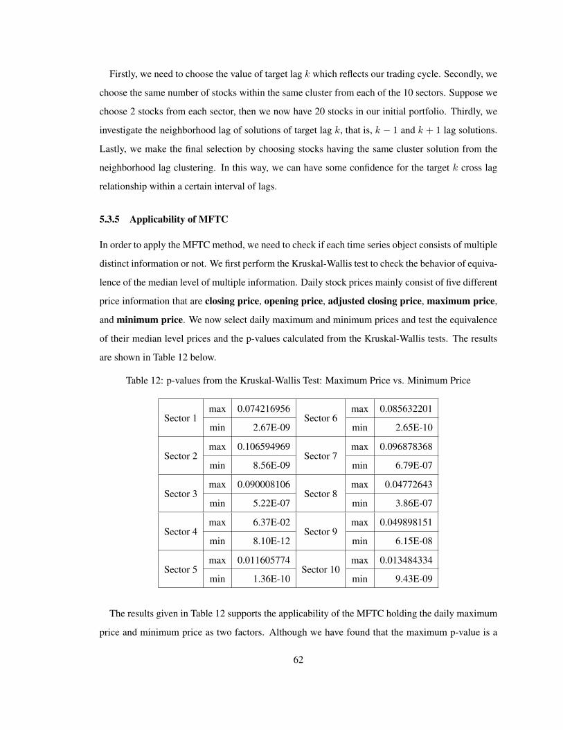
Firstly, we need to choose the value of target lag k which reflects our trading cycle. Secondly, we
choose the same number of stocks within the same cluster from each of the 10 sectors. Suppose we
choose 2 stocks from each sector, then we now have 20 stocks in our initial portfolio. Thirdly, we
investigate the neighborhood lag of solutions of target lag k, that is, k � 1 and k + 1 lag solutions.
Lastly, we make the final selection by choosing stocks having the same cluster solution from the
neighborhood lag clustering. In this way, we can have some confidence for the target k cross lag
relationship within a certain interval of lags.
5.3.5 Applicability of MFTC
In order to apply the MFTC method, we need to check if each time series object consists of multiple
distinct information or not. We first perform the Kruskal-Wallis test to check the behavior of equiva-
lence of the median level of multiple information. Daily stock prices mainly consist of five different
price information that are closing price, opening price, adjusted closing price, maximum price,
and minimum price. We now select daily maximum and minimum prices and test the equivalence
of their median level prices and the p-values calculated from the Kruskal-Wallis tests. The results
are shown in Table 12 below.
Table 12: p-values from the Kruskal-Wallis Test: Maximum Price vs. Minimum Price
Sector 1max 0.074216956
Sector 6max 0.085632201
min 2.67E-09 min 2.65E-10
Sector 2max 0.106594969
Sector 7max 0.096878368
min 8.56E-09 min 6.79E-07
Sector 3max 0.090008106
Sector 8max 0.04772643
min 5.22E-07 min 3.86E-07
Sector 4max 6.37E-02
Sector 9max 0.049898151
min 8.10E-12 min 6.15E-08
Sector 5max 0.011605774
Sector 10max 0.013484334
min 1.36E-10 min 9.43E-09
The results given in Table 12 supports the applicability of the MFTC holding the daily maximum
price and minimum price as two factors. Although we have found that the maximum p-value is a
62

little bigger than 0.1 in sector 2, which is 0.1066. If we set the level of significance, ↵, at 0.1, we can
proceed to apply MFTC method. From a stream of time dependent information, extracting multiple
distinct information is usually a very difficult process, thus, we can apply the MFTC method in the
case of selecting a p-value such as 0.1.
5.3.6 Multi-Level Clustering Result: S&P 500 Stocks - Ten Sectors
We define dissimilarity matrices at each level of the cross lag k, as we have previously discussed,
and the clustering results, using the hierarchical Ward’s clustering method, are presented below.
Table 13 presents the result of clustering based on cross lag distances. For example, the first com-
pany in sector 1, Consumer Discretionary, is “Advanced Auto Parts (AAP)” and this company
remains cluster 1 for all the cross lag distances, L0 through L10. The second company in sector 1
is “Amazon.com Inc” and this company moves between cluster 1 and cluster 2 based on the level
of lag distances. The main question at this point is how we can choose the best combination of
stocks to make profits. If you are weekly trader, you would be better to select companies based on
L7 clustering result. That is, choose companies that are in the same cluster based on L7 clustering
result. Then, we can easily find a trading point of one stock by investigating a trend of the other
stocks because they have cross lag 7 relationship. In order to find out which one proceeds the others,
we need to use one way lag distance that we are going to see in chapter 6 for the future study. In the
Table 13 below across the top are the 10 lag distance solutions, L0 to L10. The ticker is a list of all
497 companies that we are clustering with their stock market abbreviated name. Because we have
497 clustering objects, we separate the outputs by each sector and try to find the best way to build a
profitable portfolio of stocks as illustrated in previous section.
Table 13: Clustering Result for Sector 1 Companies.
Ticker L0 L1 L2 L3 L4 L5 L6 L7 L8 L9 L10
AAP 1 1 1 1 1 1 1 1 1 1 1
AMZN 1 2 2 2 2 2 1 2 2 2 2
AN 2 3 3 3 2 2 2 3 2 3 3
AZO 1 3 1 1 1 2 2 3 3 3 3
BBBY 2 4 3 4 1 3 3 4 2 1 4
63

Table 13: Clustering Result for Sector 1 Companies.
Ticker L0 L1 L2 L3 L4 L5 L6 L7 L8 L9 L10
BBY 3 3 2 2 1 2 1 3 4 4 5
BWA 1 3 1 1 1 4 4 5 2 3 3
CBS 4 5 1 2 3 2 4 3 5 1 3
CCL 1 5 3 3 1 2 2 3 2 3 2
CMCSA 1 3 3 2 2 2 4 2 4 1 5
CMG 2 2 4 5 4 5 4 1 1 3 4
COH 1 3 5 1 1 5 1 3 4 4 1
CVC 4 2 1 1 2 2 1 2 5 4 2
DG 3 6 1 1 1 2 1 3 4 4 5
DHI 1 3 3 3 3 2 1 2 4 1 2
DIS 2 3 1 1 3 1 4 3 6 2 5
DISCA 1 6 3 6 3 5 5 4 1 1 4
DISCK 4 6 3 2 1 3 5 3 1 1 4
DLPH 1 3 3 1 1 5 2 3 4 2 4
DLTR 4 3 3 1 1 2 1 2 2 4 5
DRI 1 3 6 1 1 2 3 4 3 4 4
EXPE 4 3 1 2 2 2 2 3 4 5 5
F 1 6 1 1 2 5 1 3 4 4 5
FL 4 6 1 1 5 3 3 2 4 4 1
FOX 1 6 2 3 2 2 2 3 4 4 5
FOXA 1 6 2 3 2 2 1 3 2 4 5
GM 1 6 1 3 1 2 2 3 4 1 2
GME 4 5 4 2 2 1 4 2 2 6 5
GPC 2 3 4 1 2 3 4 3 6 3 5
GPS 3 1 4 4 1 3 4 4 1 3 4
GRMN 4 3 3 1 1 5 6 2 2 2 3
GT 5 3 4 5 1 1 1 3 4 1 2
64
(Continued)

Table 13: Clustering Result for Sector 1 Companies.
Ticker L0 L1 L2 L3 L4 L5 L6 L7 L8 L9 L10
HAR 4 5 2 1 1 2 1 5 4 3 2
HAS 2 6 4 3 1 3 2 3 4 3 4
HBI 4 6 1 1 2 1 1 2 2 2 2
HD 1 6 1 3 2 2 2 2 2 4 5
HOG 4 6 1 2 2 2 1 1 5 2 4
HOT 4 2 1 1 1 5 3 3 2 2 5
IPG 5 3 3 5 3 2 4 5 2 1 2
JCI 1 5 3 3 3 5 1 1 4 3 2
JWN 2 6 1 3 1 2 1 3 4 1 5
KMX 4 3 5 1 1 2 5 5 3 2 3
KORS 3 5 4 2 1 1 5 3 4 1 4
KSS 1 1 6 1 1 5 1 1 1 6 3
LB 2 3 3 1 1 2 2 3 2 2 5
LEN 1 6 3 3 1 3 1 3 4 3 3
LOW 1 3 1 1 2 3 2 2 4 3 5
M 2 3 4 4 1 5 1 1 4 2 4
MAR 1 1 3 5 1 3 3 3 6 2 4
MAT 2 4 3 5 2 5 4 3 4 3 4
MCD 4 6 1 3 1 2 2 3 2 3 5
MHK 3 3 3 5 1 5 2 3 4 2 5
NKE 2 6 4 4 6 3 2 3 2 3 5
NWL 4 5 1 2 1 1 3 2 3 3 3
NWS 2 3 4 2 1 2 4 1 4 3 4
NWSA 2 3 3 4 3 1 4 3 1 5 4
OMC 5 6 4 5 1 2 3 1 2 3 4
ORLY 5 2 1 2 2 2 1 3 2 4 4
PCLN 1 3 3 2 1 2 4 1 2 3 2
65
(Continued)

Table 13: Clustering Result for Sector 1 Companies.
Ticker L0 L1 L2 L3 L4 L5 L6 L7 L8 L9 L10
PHM 1 3 4 5 1 1 3 3 4 6 1
PVH 4 6 1 1 2 2 5 2 2 2 3
RCL 1 2 1 3 2 1 1 2 2 2 3
RL 2 6 4 5 1 5 1 3 6 2 2
ROST 1 1 1 3 1 2 1 2 4 4 2
SBUX 5 6 1 3 2 2 1 3 6 4 5
SIG 6 3 5 6 1 6 3 6 5 3 3
SNA 1 2 1 3 1 2 1 3 2 4 2
SNI 4 5 3 1 3 1 3 1 1 3 4
SPLS 1 6 4 6 5 1 1 2 2 2 4
SWK 1 2 1 3 2 5 1 3 6 2 5
TGNA 2 3 6 5 1 2 4 3 4 5 4
TGT 2 6 1 1 1 2 4 3 4 1 5
TIF 1 5 1 5 1 5 3 6 3 1 1
TJX 1 6 1 1 3 2 5 3 4 1 5
TRIP 1 6 1 2 2 2 1 3 2 4 2
TSCO 1 6 5 1 2 2 1 2 4 2 2
TWC 1 5 1 1 2 2 1 1 2 2 5
TWX 4 6 1 2 3 2 1 1 5 3 3
UA 2 3 3 1 2 2 3 3 4 2 4
URBN 2 3 5 4 1 2 2 1 4 4 4
VFC 1 6 1 3 1 2 1 3 2 4 2
VIAB 1 5 1 1 3 2 3 3 4 3 2
WHR 1 6 1 3 3 5 1 3 3 1 1
WYN 4 2 1 1 2 5 1 1 4 2 3
WYNN 3 3 1 4 1 5 4 4 3 3 4
YUM 1 5 3 1 1 2 1 2 6 4 3
66
(Continued)

Table 14 below shows the summarized clustering output for sector 2, Consumer Staples, compa-
nies. For example, the first company in this sector is “Archer-Daniels-Midland Co (ADM)”, and
it moves dynamically from one cluster to the other clusters based on the level of cross lag distances.
If we consider a weekly trading, this company is classified to the fifth cluster. The second company
here is “ Brown-Forman Corporation (BF-B)”, and it is a member of the second cluster based on
L7 clustering.
Table 14: Clustering Result for Sector 2 Companies.
Ticker L0 L1 L2 L3 L4 L5 L6 L7 L8 L9 L10
ADM 1 3 1 2 1 5 3 5 2 3 4
BF-B 5 3 6 5 2 5 1 2 2 3 4
CAG 5 2 6 3 2 1 2 3 2 2 3
CCE 1 3 4 3 1 2 1 5 1 2 3
CHD 5 5 1 5 1 4 2 3 2 1 5
CL 1 6 1 3 2 2 2 3 2 2 5
CLX 1 6 1 3 2 2 2 3 2 2 4
COST 1 6 1 2 2 2 1 3 2 2 5
CPB 1 2 1 1 2 2 5 3 2 3 2
CVS 1 3 4 3 2 2 1 2 4 2 5
DPS 1 6 4 2 1 2 6 3 2 3 3
EL 1 2 1 3 2 2 2 2 2 4 5
GIS 5 2 1 3 1 2 2 3 2 2 5
HRL 2 2 4 1 3 2 2 3 4 2 5
HSY 5 3 6 5 3 5 2 5 4 2 4
K 5 5 1 5 1 5 2 3 2 3 5
KMB 4 3 3 2 1 2 5 3 2 3 2
KO 1 6 1 3 2 2 2 3 6 2 4
KR 1 6 1 3 1 2 1 3 6 2 2
67

Table 14: Clustering Result for Sector 2 Companies.
Ticker L0 L1 L2 L3 L4 L5 L6 L7 L8 L9 L10
MDLZ 5 3 1 5 1 5 1 5 6 2 5
MJN 4 3 1 5 3 2 1 5 2 2 4
MKC 1 6 2 3 1 2 5 2 4 2 2
MNST 1 6 1 1 2 2 2 3 5 2 5
MO 1 6 1 3 1 5 2 3 2 2 2
PEP 1 6 1 3 2 2 2 3 2 4 2
PG 1 6 6 3 3 2 2 3 2 2 4
PM 1 6 1 3 1 5 2 3 2 3 3
RAI 1 2 1 3 2 2 1 2 2 4 2
SJM 5 2 1 3 2 2 2 2 2 1 2
STZ 1 3 1 3 2 2 2 5 3 2 5
SYY 1 2 1 1 2 2 1 3 2 4 2
TAP 1 2 1 3 2 2 1 2 2 4 5
TSN 1 3 1 1 1 6 2 3 1 2 2
WBA 5 6 1 5 1 5 4 6 4 4 4
WFM 1 3 1 3 3 5 3 3 2 2 2
WMT 1 2 1 3 1 2 2 2 4 4 5
In Table 15 below, we find the clustering results for sector 3, Energy, companies. For exam-
ple, the first company in this sector is “Anadarko Petroleum Corp (APC)”, and we see that this
company belongs to the cluster 5 if we assume a weekly trading.
Table 15: Clustering Result for Sector 3 Companies.
Ticker L0 L1 L2 L3 L4 L5 L6 L7 L8 L9 L10
APA 3 4 3 4 3 2 4 5 4 3 1
68
(Continued)

Table 15: Clustering Result for Sector 3 Companies.
Ticker L0 L1 L2 L3 L4 L5 L6 L7 L8 L9 L10
APC 3 4 6 5 4 6 4 4 4 3 4
BHI 1 5 6 5 3 4 4 4 4 5 6
CHK 6 3 6 5 4 4 4 6 3 5 1
COG 3 4 6 5 2 5 6 6 3 3 4
COP 1 2 6 5 3 6 2 5 4 5 4
CVX 4 5 6 5 3 6 1 2 2 3 3
CXO 6 3 3 6 5 4 4 6 3 5 3
DO 3 6 5 6 3 6 4 3 2 2 1
DVN 3 4 2 5 4 6 4 5 1 3 6
EOG 3 4 1 5 3 6 4 5 3 3 3
EQT 3 1 4 4 4 5 4 1 3 3 1
FTI 3 4 6 4 3 5 4 3 1 4 1
HAL 3 4 1 5 3 5 4 3 1 5 1
HES 3 4 1 4 3 6 4 5 3 3 1
HP 3 3 3 5 3 6 4 5 4 3 3
KMI 1 1 6 4 1 5 4 1 1 3 4
MPC 2 5 4 3 2 1 1 3 4 3 2
MRO 3 4 4 5 4 6 4 4 1 5 3
MUR 4 4 6 5 3 6 4 3 3 3 3
NBL 3 4 6 5 4 6 3 5 1 3 4
NFX 3 5 3 1 3 5 4 2 1 6 4
NOV 2 3 1 5 5 2 4 1 4 4 2
OKE 6 1 6 2 3 4 3 6 1 3 3
OXY 1 3 1 5 4 6 4 3 3 3 1
PSX 2 6 4 5 3 5 2 5 4 3 4
PXD 6 6 6 3 3 6 4 5 3 5 1
RIG 3 1 4 6 3 5 4 4 1 5 1
69
(Continued)

Table 15: Clustering Result for Sector 3 Companies.
Ticker L0 L1 L2 L3 L4 L5 L6 L7 L8 L9 L10
RRC 6 1 6 2 3 4 6 5 3 3 4
SE 3 3 6 5 3 6 4 4 1 3 1
SLB 4 1 6 5 2 5 4 3 3 2 4
SWN 6 4 6 6 4 4 3 6 3 3 1
TSO 6 3 1 2 3 2 2 5 3 3 4
VLO 2 3 1 5 3 5 2 5 2 3 4
WMB 6 5 5 2 4 4 3 4 3 1 6
XEC 3 3 6 4 4 4 4 4 4 5 4
XOM 1 6 1 3 3 6 4 3 5 2 4
Table 16 below is the clustering output for sector 4, Financials, companies. For example, the
first company in this sector is “AFLAC Inc (AFL)”, and this company belongs to the third cluster
based on L7 cross lag distances.
Table 16: Clustering Result for Sector 4 Companies.
Ticker L0 L1 L2 L3 L4 L5 L6 L7 L8 L9 L10
AFL 1 2 1 3 2 2 1 3 6 2 4
AIG 1 2 5 3 1 2 1 3 6 4 3
AIV 1 6 2 1 2 2 1 2 5 2 2
AIZ 4 3 1 3 3 2 1 3 4 4 2
ALL 1 6 2 5 3 5 1 1 6 4 5
AMG 4 3 3 2 3 1 3 5 4 5 1
AMP 2 2 6 5 2 5 5 3 6 2 4
AMT 2 3 4 1 3 2 1 3 4 4 2
AON 1 6 1 3 1 2 1 3 6 6 2
70
(Continued)

Table 16: Clustering Result for Sector 4 Companies.
Ticker L0 L1 L2 L3 L4 L5 L6 L7 L8 L9 L10
AVB 4 6 1 1 2 1 6 2 5 4 2
AXP 1 2 1 3 2 2 1 3 6 2 2
BAC 1 2 1 5 3 2 6 3 6 2 4
BBT 1 2 1 3 3 2 6 3 6 4 4
BEN 1 3 6 1 3 2 5 5 4 1 2
BK 4 2 1 1 1 2 6 3 4 6 4
BLK 4 3 1 2 2 1 5 3 6 2 3
BRK-B 1 6 1 3 2 2 1 3 6 4 2
BXP 1 3 1 1 3 2 1 2 5 2 1
C 1 2 1 3 2 2 1 3 4 2 2
CB 2 2 1 1 1 2 4 3 6 4 4
CBG 1 2 6 3 3 2 1 3 2 4 4
CCI 1 6 2 1 2 2 6 2 5 4 5
CFG 4 3 1 1 1 2 1 3 4 4 4
CINF 5 2 1 1 2 5 1 3 2 4 3
CMA 4 5 1 1 3 2 1 5 4 4 4
CME 1 1 6 5 3 5 6 3 4 4 4
COF 4 6 1 1 2 2 1 3 6 2 4
DFS 1 6 1 3 2 1 1 3 2 2 4
EFX 1 6 1 1 3 2 1 3 2 2 3
EQR 4 2 2 1 2 2 2 2 2 4 2
ESS 4 2 2 1 2 1 1 2 5 4 3
ETFC 4 3 1 2 3 2 1 3 4 4 2
EXR 1 2 3 1 2 5 1 2 2 4 2
FITB 4 3 1 3 3 1 1 3 3 6 2
FRT 4 6 2 6 3 1 1 2 2 4 4
GGP 1 1 1 1 3 1 1 2 2 4 3
71
(Continued)
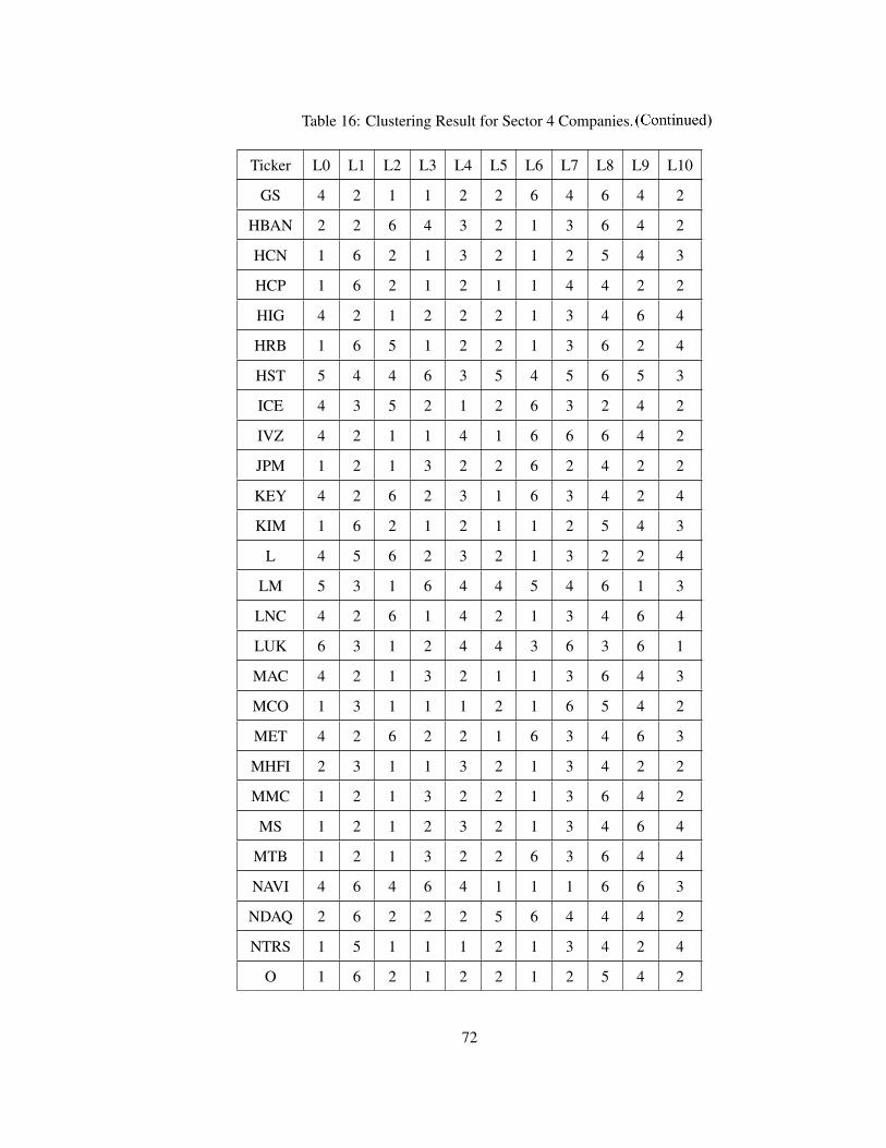
Table 16: Clustering Result for Sector 4 Companies.
Ticker L0 L1 L2 L3 L4 L5 L6 L7 L8 L9 L10
GS 4 2 1 1 2 2 6 4 6 4 2
HBAN 2 2 6 4 3 2 1 3 6 4 2
HCN 1 6 2 1 3 2 1 2 5 4 3
HCP 1 6 2 1 2 1 1 4 4 2 2
HIG 4 2 1 2 2 2 1 3 4 6 4
HRB 1 6 5 1 2 2 1 3 6 2 4
HST 5 4 4 6 3 5 4 5 6 5 3
ICE 4 3 5 2 1 2 6 3 2 4 2
IVZ 4 2 1 1 4 1 6 6 6 4 2
JPM 1 2 1 3 2 2 6 2 4 2 2
KEY 4 2 6 2 3 1 6 3 4 2 4
KIM 1 6 2 1 2 1 1 2 5 4 3
L 4 5 6 2 3 2 1 3 2 2 4
LM 5 3 1 6 4 4 5 4 6 1 3
LNC 4 2 6 1 4 2 1 3 4 6 4
LUK 6 3 1 2 4 4 3 6 3 6 1
MAC 4 2 1 3 2 1 1 3 6 4 3
MCO 1 3 1 1 1 2 1 6 5 4 2
MET 4 2 6 2 2 1 6 3 4 6 3
MHFI 2 3 1 1 3 2 1 3 4 2 2
MMC 1 2 1 3 2 2 1 3 6 4 2
MS 1 2 1 2 3 2 1 3 4 6 4
MTB 1 2 1 3 2 2 6 3 6 4 4
NAVI 4 6 4 6 4 1 1 1 6 6 3
NDAQ 2 6 2 2 2 5 6 4 4 4 2
NTRS 1 5 1 1 1 2 1 3 4 2 4
O 1 6 2 1 2 2 1 2 5 4 2
72
(Continued)

Table 16: Clustering Result for Sector 4 Companies.
Ticker L0 L1 L2 L3 L4 L5 L6 L7 L8 L9 L10
PBCT 1 2 1 1 3 2 6 4 2 4 5
PFG 4 5 6 3 2 2 3 3 6 6 3
PGR 5 3 6 3 2 5 6 3 6 2 4
PLD 1 2 2 3 2 2 1 2 2 4 2
PNC 1 2 1 3 2 2 1 2 2 2 2
PRU 1 2 1 3 3 2 6 3 4 6 2
PSA 1 6 2 6 2 5 1 2 5 4 5
RF 4 2 6 5 3 2 6 4 4 4 2
SCHW 4 2 1 1 3 1 6 3 4 4 2
SLG 2 6 4 4 3 1 4 3 4 4 5
SPG 4 6 1 1 3 1 1 2 2 4 5
STI 1 2 1 5 3 2 6 3 4 4 2
STT 4 2 1 2 3 1 5 1 6 6 1
SYF 4 6 2 3 3 1 6 3 4 2 4
TMK 4 2 1 1 3 2 3 3 2 1 2
TROW 2 6 3 3 3 6 1 3 4 4 2
TRV 1 6 1 3 2 2 1 3 6 4 2
TW 1 4 3 3 2 2 1 3 5 2 2
UDR 5 1 2 6 3 1 1 2 1 6 3
UNM 5 3 6 2 3 1 1 3 4 6 3
USB 1 6 1 1 2 2 1 3 4 2 2
VNO 1 2 2 1 2 1 1 2 2 3 3
VTR 4 6 2 3 1 1 2 2 2 4 3
WFC 1 2 1 3 2 2 1 3 2 4 2
WY 5 1 6 4 3 2 1 3 6 2 1
XL 1 2 1 3 2 1 1 3 6 4 2
ZION 4 3 5 3 3 2 6 4 4 4 4
73
(Continued)

Table 17 gives the clustering solutions for sector 5, Health Care, companies. For example, the
first company in this sector is “Agilent Technologies Inc (A)”, and this company belongs to the
second cluster based on L7 clustering.
Table 17: Clustering Result for Sector 5 Companies.
Ticker L0 L1 L2 L3 L4 L5 L6 L7 L8 L9 L10
A 4 3 1 1 3 2 6 2 4 4 3
ABBV 1 6 1 1 3 2 1 2 4 2 2
ABC 4 3 1 5 2 1 2 3 2 4 2
ABT 2 6 1 3 1 2 1 3 4 4 2
AET 2 4 1 5 2 2 1 1 5 2 3
AGN 1 3 2 1 1 1 1 3 5 4 1
ALXN 4 6 2 2 2 1 6 1 5 4 2
AMGN 4 3 6 2 1 2 4 2 5 6 6
ANTM 1 1 1 1 5 2 1 1 4 6 1
BAX 4 2 1 1 2 1 5 2 2 4 2
BCR 1 3 2 1 2 1 1 3 4 5 3
BDX 2 6 1 1 2 2 1 2 2 4 5
BIIB 1 3 1 6 5 1 1 3 5 4 2
BMY 4 6 1 1 2 1 1 2 6 4 2
BSX 1 6 1 3 2 2 2 1 6 4 2
CAH 1 2 1 1 2 2 1 2 2 4 2
CELG 4 6 1 2 3 4 2 2 5 4 2
CERN 2 6 4 4 3 2 5 3 6 4 2
CI 4 2 1 1 3 1 1 2 2 4 2
CNC 1 6 1 3 2 2 1 3 3 4 2
DGX 1 6 1 1 2 2 1 3 5 4 2
DVA 1 2 1 3 2 2 1 6 4 4 5
74

Table 17: Clustering Result for Sector 5 Companies.
Ticker L0 L1 L2 L3 L4 L5 L6 L7 L8 L9 L10
ENDP 4 6 6 6 3 5 6 2 4 4 4
ESRX 1 2 1 3 3 2 3 3 6 4 5
EW 1 6 1 3 2 2 1 3 2 2 2
GILD 1 6 1 5 2 1 1 3 6 2 2
HCA 4 6 1 3 2 2 1 2 6 2 2
HOLX 5 6 3 2 5 2 1 2 2 2 5
HSIC 4 6 1 1 2 2 1 3 2 4 5
HUM 1 2 1 1 1 1 5 2 6 4 3
ILMN 2 4 6 1 5 2 1 3 4 4 1
ISRG 4 6 6 2 3 2 1 2 2 2 4
JNJ 1 2 1 3 2 2 1 2 6 4 5
LH 1 6 1 3 2 1 1 2 5 4 3
LLY 5 4 1 4 5 6 1 5 2 4 2
MCK 4 6 1 1 2 2 1 3 3 2 2
MDT 1 2 1 3 2 2 2 2 2 4 2
MNK 3 3 4 6 4 6 4 4 1 5 1
MRK 1 3 5 3 1 1 1 2 2 4 2
MYL 2 6 5 5 3 2 1 3 1 6 2
PDCO 1 2 1 3 2 2 1 2 2 4 6
PFE 1 3 1 3 2 1 1 3 2 2 2
PKI 4 6 1 1 2 1 6 5 4 2 3
PRGO 2 6 4 1 3 2 1 3 4 2 2
REGN 4 3 3 2 5 6 4 1 4 2 2
STJ 4 6 6 1 2 1 1 1 2 4 3
SYK 2 6 2 1 2 2 1 3 6 4 2
THC 3 1 4 6 4 5 4 4 1 4 4
TMO 1 6 6 1 2 2 1 3 6 4 3
75
(Continued)

Table 17: Clustering Result for Sector 5 Companies.
Ticker L0 L1 L2 L3 L4 L5 L6 L7 L8 L9 L10
UHS 1 5 6 1 2 1 3 1 5 4 3
UNH 1 6 1 3 2 2 1 3 6 4 2
VAR 1 6 1 3 1 2 1 3 2 4 2
VRTX 4 4 3 6 3 6 6 1 6 6 2
WAT 1 6 5 5 2 6 1 2 4 4 2
XRAY 4 4 5 1 3 2 1 2 6 4 2
ZBH 4 2 1 3 2 2 6 2 2 4 3
ZTS 1 6 1 3 2 2 1 2 2 4 2
Table 18 below shows clustering solutions for sector 6, Industrials, companies. For example, the
first company in this sector is “American Airlines Group (AAL)”, and this company is a member
of cluster 4 based on L7 clustering output.
Table 18: Clustering Result for Sector 6 Companies.
Ticker L0 L1 L2 L3 L4 L5 L6 L7 L8 L9 L10
AAL 3 3 1 5 3 5 4 4 4 5 1
ADT 3 5 4 2 5 2 4 4 4 4 2
ALLE 5 3 2 1 5 1 5 3 6 6 2
AME 1 6 1 3 2 2 1 2 4 4 2
APH 1 6 1 1 2 2 1 3 2 2 2
BA 2 2 2 2 2 2 1 3 6 4 2
CAT 1 4 4 5 3 5 6 3 4 6 2
CHRW 2 6 1 4 2 6 1 3 6 4 1
CMI 4 3 4 2 3 1 5 3 4 4 2
COL 2 3 1 2 2 1 6 3 6 4 2
76
(Continued)

Table 18: Clustering Result for Sector 6 Companies.
Ticker L0 L1 L2 L3 L4 L5 L6 L7 L8 L9 L10
CSX 4 1 6 2 4 6 6 2 4 6 2
CTAS 1 6 6 3 2 5 6 3 2 1 2
DAL 2 3 2 2 3 1 4 5 4 4 2
DE 2 6 4 2 2 5 2 3 6 4 2
DHR 1 2 1 3 2 2 6 3 1 4 2
DNB 2 6 1 5 3 5 1 3 6 4 4
DOV 1 4 6 5 2 1 6 3 4 3 3
EMR 4 4 6 5 3 4 1 3 4 4 3
ETN 1 6 6 2 3 1 6 3 1 4 2
EXPD 1 6 5 1 3 2 1 3 6 2 2
FAST 5 6 6 5 5 1 6 3 6 4 2
FDX 4 2 1 2 5 2 1 3 4 4 2
FLIR 2 6 1 3 2 1 4 3 4 3 2
FLR 2 2 4 5 3 5 6 2 1 4 1
FLS 1 4 6 5 3 1 6 3 1 4 1
GD 5 2 4 3 2 2 1 1 6 2 2
GE 4 2 1 1 2 2 1 2 2 2 2
GLW 1 6 4 3 3 6 1 5 6 4 2
GWW 1 6 1 3 5 5 6 3 2 4 5
HON 2 2 1 3 2 2 2 5 6 4 2
IR 2 6 1 3 2 1 6 2 6 2 2
IRM 2 6 4 4 3 1 4 1 6 2 1
ITW 2 6 4 5 2 1 6 3 6 4 2
JBHT 4 1 5 2 3 1 6 6 5 4 2
JEC 1 6 4 5 4 4 6 3 1 6 2
KSU 4 6 1 2 4 6 1 6 5 6 3
LEG 2 2 1 3 1 2 1 3 6 4 2
77
(Continued)

Table 18: Clustering Result for Sector 6 Companies.
Ticker L0 L1 L2 L3 L4 L5 L6 L7 L8 L9 L10
LLL 1 1 1 3 2 1 1 1 4 1 2
LMT 5 6 1 3 2 1 6 2 6 2 2
LUV 2 1 4 5 1 5 1 1 4 1 2
MAS 5 2 1 3 1 1 1 1 5 6 2
MMM 2 6 4 3 3 2 1 3 2 4 4
NLSN 1 6 4 1 3 2 1 2 6 2 2
NOC 5 5 1 3 3 2 1 1 6 2 5
NSC 4 1 4 2 5 1 1 3 4 6 1
PBI 1 6 6 2 3 4 6 2 4 4 1
PCAR 2 3 4 3 2 5 6 5 6 4 2
PH 2 4 4 5 5 5 6 5 4 6 1
PNR 4 4 6 5 3 4 6 3 1 1 1
PWR 2 4 4 5 3 6 4 5 1 5 1
R 4 3 4 6 4 1 6 4 5 6 2
RHI 1 5 5 4 5 1 6 3 1 4 2
ROK 2 6 1 3 5 2 5 3 4 6 2
ROP 2 6 1 1 2 2 1 2 4 4 2
RSG 1 2 1 3 2 2 1 2 6 4 2
RTN 5 6 1 3 2 1 1 2 6 4 3
SRCL 1 6 1 3 2 2 1 3 2 4 2
TXT 1 2 1 3 3 2 1 3 1 4 1
TYC 2 5 5 2 5 5 6 3 4 4 2
UAL 3 4 4 4 4 5 3 1 1 5 6
UNP 4 6 1 2 1 1 6 2 2 6 2
UPS 1 6 1 2 2 2 1 3 6 6 2
URI 1 6 4 3 5 2 5 2 5 1 1
UTX 1 6 5 3 2 2 1 3 6 4 2
78
(Continued)

Table 18: Clustering Result for Sector 6 Companies.
Ticker L0 L1 L2 L3 L4 L5 L6 L7 L8 L9 L10
VRSK 1 6 1 3 3 5 1 3 4 2 2
WM 1 1 1 3 2 2 1 1 2 4 2
XYL 2 4 1 5 1 1 6 3 1 4 1
Table 19 below includes the lag clustering solutions for sector 7, Information Technology, com-
panies. For example, the first company shown in this table is “Apple Inc (AAPL)”, and this com-
pany belongs to the cluster 4 based on L7 lag distances.
Table 19: Clustering Result for Sector 7 Companies.
Ticker L0 L1 L2 L3 L4 L5 L6 L7 L8 L9 L10
AAPL 5 2 1 3 3 1 5 4 6 6 2
ACN 1 2 6 3 2 2 1 2 1 2 2
ADBE 4 2 6 2 2 2 1 3 6 2 2
ADI 1 2 6 2 2 5 6 3 6 6 6
ADP 5 2 1 2 2 2 5 3 6 6 2
ADS 1 2 1 2 3 2 6 2 5 4 2
ADSK 5 4 5 2 5 1 2 1 6 6 3
AKAM 4 2 5 1 3 2 1 2 6 4 2
AMAT 2 6 4 6 4 1 1 3 4 2 2
ATVI 5 6 5 5 1 2 1 2 6 2 3
AVGO 4 6 6 3 1 5 6 1 4 1 4
CA 5 2 6 5 2 1 6 1 6 6 2
CRM 1 1 1 3 2 1 1 3 2 4 2
CSCO 2 6 1 3 2 2 5 1 6 4 2
CTSH 5 6 1 3 3 2 2 3 6 2 3
79
(Continued)

Table 19: Clustering Result for Sector 7 Companies.
Ticker L0 L1 L2 L3 L4 L5 L6 L7 L8 L9 L10
CTXS 2 6 5 5 4 4 4 1 6 4 6
EA 2 1 1 4 1 1 1 1 6 4 2
EBAY 1 6 2 3 2 2 1 2 6 4 2
EMC 1 6 1 3 2 2 1 2 4 4 2
EQIX 4 5 1 2 5 1 2 1 2 6 3
FB 1 1 4 2 3 1 1 1 2 4 2
FFIV 2 5 1 4 1 2 1 3 1 4 1
FIS 1 1 2 1 3 2 1 2 1 1 2
FISV 5 2 1 2 2 2 1 3 6 2 3
FSLR 3 6 4 5 3 5 1 5 6 4 1
GOOG 1 6 6 2 2 2 6 5 2 2 5
GOOGL 1 6 4 2 2 1 6 5 6 2 5
HPQ 4 3 1 1 3 2 6 3 5 2 5
HRS 1 2 1 3 5 2 2 2 4 4 2
IBM 1 6 1 2 3 5 3 3 6 2 2
INTC 1 6 1 3 5 5 1 1 6 3 1
INTU 5 2 5 2 2 2 2 1 6 2 5
JNPR 1 6 4 1 1 2 1 3 2 2 2
KLAC 1 2 1 3 2 2 6 2 6 2 2
LLTC 5 6 6 2 5 1 4 1 6 6 2
LRCX 1 3 2 2 5 1 2 1 4 4 2
MA 1 2 5 3 2 2 1 3 6 2 2
MCHP 5 1 6 2 2 1 1 1 4 6 2
MSFT 1 6 1 2 2 5 2 3 6 4 3
MSI 1 2 1 3 2 2 1 3 6 2 2
MU 1 5 3 2 3 4 6 1 4 4 1
NFLX 5 2 1 3 2 2 1 1 6 2 3
80
(Continued)

Table 19: Clustering Result for Sector 7 Companies.
Ticker L0 L1 L2 L3 L4 L5 L6 L7 L8 L9 L10
NTAP 1 6 5 5 5 1 3 1 4 6 3
NVDA 1 6 1 2 2 2 1 2 4 6 2
ORCL 1 2 4 5 2 1 1 2 1 6 2
PAYX 5 2 1 3 3 5 5 3 6 6 3
QCOM 2 6 6 3 1 2 1 3 4 6 6
QRVO 5 4 6 6 4 1 3 1 6 5 2
RHT 1 6 5 1 5 1 4 1 5 4 2
SNDK 1 2 1 3 2 1 1 3 5 4 2
STX 1 1 4 5 3 5 5 4 4 6 1
SWKS 5 4 6 6 3 4 3 1 6 6 4
SYMC 2 1 1 2 2 2 1 1 4 4 3
TDC 2 5 4 5 1 5 1 2 1 6 4
TEL 1 2 1 3 2 2 1 3 6 4 3
TSS 2 2 1 3 1 5 1 3 1 2 2
TXN 5 4 6 5 4 1 6 1 4 6 6
V 4 2 1 3 2 2 2 3 6 4 5
VRSN 1 6 1 3 1 1 1 2 2 4 2
WDC 1 5 4 3 5 4 5 4 6 6 1
WU 5 5 1 3 5 1 1 1 6 2 2
XLNX 5 6 6 1 2 1 1 1 6 2 6
XRX 1 1 4 6 3 5 3 1 6 6 2
YHOO 2 2 6 4 2 2 5 3 6 4 4
Table 20 below shows the clustering solutions for sector 8, Materials, companies. For example,
the company listed first is “Alcoa Inc (AA)”, and the second cluster includes this company when
we consider L7 lag distances.
81
(Continued)

Table 20: Clustering Result for Sector 8 Companies.
Ticker L0 L1 L2 L3 L4 L5 L6 L7 L8 L9 L10
AA 4 1 3 5 2 4 6 2 5 4 3
APD 5 6 1 3 2 2 1 1 2 2 6
ARG 4 6 1 3 2 2 1 2 2 4 5
AVY 1 6 5 4 2 2 1 3 2 4 2
BLL 2 1 1 1 2 1 1 3 6 4 2
CF 3 1 4 3 3 5 4 3 4 4 6
DD 4 2 5 3 2 1 2 1 2 4 2
DOW 2 6 1 3 2 2 1 4 4 4 6
ECL 1 1 1 2 3 1 1 3 6 6 2
EMN 1 1 1 3 3 4 1 1 1 4 6
FCX 4 1 6 6 4 4 6 5 1 6 2
FMC 5 1 1 4 3 5 6 5 4 6 2
IFF 2 5 5 3 5 2 1 1 6 4 1
IP 2 6 4 4 4 5 5 3 4 4 2
LYB 1 6 1 4 1 1 6 3 1 4 2
MLM 1 5 1 4 2 1 1 3 1 4 6
MON 1 6 6 3 5 1 6 3 5 6 2
MOS 3 1 4 4 4 6 1 4 4 6 6
NEM 4 4 6 6 4 5 6 6 1 6 6
NUE 4 3 1 6 4 4 3 6 3 4 6
OI 1 3 4 4 4 1 4 4 1 4 3
PPG 1 2 1 3 2 2 1 3 5 4 2
PX 1 1 4 3 5 1 1 3 1 2 6
SEE 2 6 5 2 5 6 1 1 4 4 4
SHW 2 5 1 4 2 1 4 1 1 6 2
VMC 1 1 4 2 5 2 1 1 5 4 1
82

In Table 21, we present the clustering solutions for sector 9, Telecommunications Services,
companies. For example, we find the company “CenturyLink Inc (CTL)” at the first row in the
table, and this company belongs to the cluster 3 based on L7 lag distances.
Table 21: Clustering Result for Sector 9 Companies.
Ticker L0 L1 L2 L3 L4 L5 L6 L7 L8 L9 L10
CTL 3 1 6 4 3 5 1 2 2 4 1
FTR 3 5 4 4 4 5 4 4 1 4 1
LVLT 4 6 5 1 5 1 6 1 2 4 3
T 2 6 5 3 2 2 5 1 1 4 2
VZ 2 2 4 3 1 1 5 1 6 4 2
The last solution shown in Table 22 is the output for sector 10, Utilities, companies. For example,
the first listed company in this sector is “American Corp (AEE)”, and this company belongs to the
first cluster based on L7 lag distances.
Table 22: Clustering Result for Sector 10 Companies.
Ticker L0 L1 L2 L3 L4 L5 L6 L7 L8 L9 L10
AEE 5 1 6 2 1 5 5 1 1 6 6
AEP 5 5 5 2 4 4 2 1 6 6 1
AES 5 3 6 6 4 6 6 6 1 1 6
AWK 4 2 1 2 5 5 1 2 2 5 6
CMS 5 5 5 2 5 4 5 1 6 1 3
CNP 4 5 1 1 5 1 2 1 2 1 3
D 5 1 5 2 2 5 5 1 2 6 6
DTE 5 5 5 6 5 4 5 1 2 1 3
83

Table 22: Clustering Result for Sector 10 Companies.
Ticker L0 L1 L2 L3 L4 L5 L6 L7 L8 L9 L10
DUK 5 2 1 6 4 4 5 4 6 3 1
ED 5 1 1 2 1 4 1 1 6 1 3
EIX 5 5 5 2 5 5 5 1 6 6 3
ES 5 5 3 2 5 4 5 1 6 5 6
ETR 5 5 5 6 1 5 3 4 4 1 3
EXC 1 2 2 2 5 1 5 4 5 6 6
FE 5 5 1 6 5 4 3 1 6 1 6
GAS 1 2 1 3 2 2 2 2 2 4 5
NEE 4 2 5 3 1 4 5 1 6 6 1
NI 4 2 1 1 2 1 5 2 2 4 3
NRG 6 3 6 6 4 4 3 6 3 1 3
PCG 5 5 5 1 5 4 5 1 2 1 3
PEG 5 5 1 6 3 6 5 1 6 5 6
PNW 5 5 3 2 5 1 5 1 6 1 3
PPL 4 2 1 2 5 4 5 1 6 1 6
SCG 5 5 4 2 1 4 2 1 2 5 3
SO 5 5 1 2 5 4 5 1 2 1 3
SRE 2 5 4 2 4 4 1 2 6 5 6
TE 1 2 1 3 2 2 1 3 2 4 5
WEC 5 1 4 5 5 1 5 1 6 6 3
XEL 4 5 5 2 1 4 5 1 6 6 3
Thus, one can utilize the clustering results of our algorithm to make constructive decision with
respect to a diversified portfolio based on their objectives.
84
(Continued)

5.4 Structuring a Portfolio
Let us consider that a portfolio manger wants to structure a diversified portfolio by selecting one
stock from each of 10 business sectors among S&P 500 companies. In order to fulfill his strategy,
we can utilize the MLTC algorithm to structure such a diversified portfolio, and Table 23 below
displays an example of such a portfolio that is put together by utilizing the MLTC results presented
in Table 13 through Table 22.
Table 23: Portfolio Selection.
Sector Selected Ticker L6 L7 L8
Consumer Discretionary AMZN 1 2 2
Consumer Staples BF-B 1 2 2
Energy CVX 1 2 2
Financials EXR 1 2 2
Health Care BDX 1 2 2
Industrials GE 1 2 2
Information Technology VRSN 1 2 2
Materials ARG 1 2 2
Telecommunications Services CTL 1 2 2
Utilities AWK 1 2 2
The selected portfolio shown in Table 23 is based on Figure 29, the MLTC Procedure, and we
have applied k = 7, that is, we have assumed the trading interval as a week. The structured portfolio
in Table 23 also shows that all the selected stocks have the same lag solutions for the neighborhood
clustering results, L6 and L8.
The portfolio manger now have the structure of the portfolio based on his strategy as shown in
Figure 30. The equal angles for all 10 sectors in Figure 30 does not imply the equal number of
stocks, it indicates the equal amount of investment, and the portfolio manger is not restricted to
85

Figure 30.: Structure of the Selected Portfolio.
have the equal amount investment strategy. The portfolio manger will be able to modify the amount
of investment in each sector easily based on the behavior of the current stock market.
5.5 Conclusion / Contributions
We have developed an algorithm for clustering time series data of the prices of stocks using the
MLTC method. We have introduced a step-by-step procedure on implementing this MLTC driven
algorithm. We have shown how this procedure works by using 497 stocks from S&P 500 to cluster
them according to 10 business sectors. The clustering solutions based on L0 (lag 0 distances)
through L10 (lag 10 distances) for all 497 companies in 10 GICS sectors.
Now, we illustrate how an investor can combine solutions from all 10 business sectors. If an
individual is a weekly trader in the stock market, then first, he has to select the same number of
86

companies in each sector based on L7 solutions for quality and diversification. Now you have 20
companies that you are considering and if you consider two companies from each sector, and all of
them have cross lag 7 relationship, that is, all 20 companies’ stock prices tend to catch tails each
other in 7 days’ interval. After you choose stocks based on L7 solutions, you need to investigate
further on L6 and L8 solutions to see if they all are in the same cluster based on adjacent lag
distances. If you find stocks that are also in the same cluster based on adjacent lag distance solutions,
then those stocks may build the best portfolio because their price behaviors based on the level of lag
distances are similar over desired trading period and we have a wider confidence for those stocks.
87

Chapter 6
Future Research
6.1 Solutions to the Global Warming Problem in South Korea
We want to perform a surface response analysis to answer the following question. If South Korea
is interested in identifying the amount of each of the attributable variables so as to minimize CO2
in the atmosphere, or to be at a certain desirable level. We will be able to do this by performing
the surface response analysis on the developed nonlinear statistical model. That is, we want to be
at least 95% or 90% certain that if we confine the amount that each one of the attributable variables
contribute along with interactions, then we will be sure that CO2 meets a certain level that has
been identified by legal policies. Therefore, in order to do this, we use the methodology of surface
response analysis. Again, we want to meet a certain level of CO2 output so that want to be able
to identify the amount that each attributable variable is allowed to produce so as to be at least 95%
certain that CO2 in the atmosphere meets the standards.
In addition, we want to study the number one attributable variable which is Liquid Fuels and
structure a differential equation that characterizes the behavior of Liquid Fuels, and knowing that
at any particular time in the present or future, we can obtain the solution to the differential equa-
tion where we can put a specific time to see whether atmospheric CO2 decreases, stays the same,
or increases. This is important information to constantly monitoring the behavior of CO2 in the
atmosphere.
6.2 Extension of LTTC, MFTC, and MLTC Methods
In the present study, we have discussed the importance of clustering time dependent information
and proposed new methods to cluster time dependent information. The proposed methods produce
clustering solutions that are probabilistically determined based on our objective of the study. There-
fore, we believe that we will be able to introduce Bayesian Paradigm to the clustering procedure,
88

especially in the case of MLTC to improve its effectiveness. We also want to apply these methods
to data from various fields of studies.
6.3 Applications
We intend to apply the proposed active and dynamic methods that we have developed to other
interesting problems in finance, ecology, psychology, among others.
89

References
[1] W. F. Velicer, Suppressor Variables and the Semipartial Correlation Coefficient, Educational
and Psychological Measurement 38 (4) (1978), pp. 953-958.
[2] T. A. Boden, G. Marland and R. J. Andres, Global, regional, and national fossil-fuel CO2
emissions, CDIAC (2011).
[3] A. C. Davison and C. L. Tsai, Regression model diagnostics, International Statistical Review
60 (3) (1992), pp. 337-353.
[4] Nicholas R. Farnum, Using Johnson curves to describe non-normal process data, Quality
Engineering 9 (2) (1997), pp. 329-336.
[5] K. Hackett and C. P. Tsokos, A new method for obtaining a more effective estimation of atmo-
spheric temperature in the contiguous United States, Nonlinear Analysis: Theory, Methods &
Applications 71 (12) (2009), pp. e1153-e1159.
[6] Douglas MacKinnon, Global-warming zealots reap huge profits from peddling their phony
settled science, The Tampa Tribune (Aug 7, 2014).
[7] Richard Schmalensee, Thomas M. Stoker, and Ruth A. Judson, World carbon dioxide emis-
sions: 1950-2050, The Review of Economics and Statistics 80 (1) (1998), pp. 15-27.
[8] Science and Technology, Climate Science: A Sensitive Matter: The climate may be heating up
less in response to green-house-gas emissions than was once thought. But that does not mean
the problem is going away, The Economist (Mar 30, 2013).
[9] S. H. Shih and C. P. Tsokos, A temperature forecasting model for the continental United States,
J. Neural, Parallel & Scientific Computations 16 (1) (2008), pp. 59-72.
90

[10] S. H. Shih and C. P. Tsokos, Prediction model for carbon dioxide emission in the atmosphere,
J. Neural, Parallel & Scientific Computations 16 (1) (2008), pp. 165-178.
[11] I. Teodorescu and C. P. Tsokos, Contributors of carbon dioxide in the atmosphere in Europe,
arXiv:1312.7867v1 (2013) (stat.CO).
[12] I. Teodorescu and C. P. Tsokos, Contributors of carbon dioxide in the atmosphere in Europe:
The surface response analysis, arXiv:1401.0087v1 (2013) (stat.AP).
[13] C. P. Tsokos, Statistical modeling of global warming, The 5th International Conference on
Dynamic Systems and Applications 5 (1) (2008), pp. 461-466.
[14] C. P. Tsokos, Global warming: Myth and reality, Hellenic News of America 23 (3) (2009),
pp. 1-3.
[15] C. P. Tsokos and Y. Xu, Modeling carbon dioxide emission with a system of differential equa-
tions, International Encyclopedia of Statistical Science 71 (12) (2009), pp. e1182-e1197.
[16] C. P. Tsokos, Mathematical and statistical modeling of global warming, Hellenic News of
America (2011), pp. 781-786.
[17] R. Wooten and C. P. Tsokos, Parametric analysis of carbon dioxide in the atmosphere, Journal
of Applied Sciences 10 (6) (2010), pp. 440-450.
[18] Ernst Worrell et al., Carbon dioxide emissions from the global cement industry, Annual Review
of Energy and the Environment 26 (1) (2001), pp. 303-329.
[19] Y. Xu and C. P. Tsokos, Statistical models and analysis of carbon dioxide in the atmosphere,
Problems of Nonlinear Analysis in Engineering Systems 2 (36) (2011), pp. e1.
[20] Y. Xu and C. P. Tsokos, Attributable variables with interactions that contribute to carbon
dioxide in the atmosphere, Frontiers in Science 2 (1) (2013), pp. 6-13.
[21] C. P. Tsokos, Statistical Modeling of Global Warming, Fifth International Conference on Dy-
namical Systems and Applications, Morehouse College, Atlanta, GA, May 30, 2008
91

[22] C. P. Tsokos, Global Warming: Myth, Reality, Copenhagen and Developments, The Fourth
International Conference on Neural, Parallel and Scientific Computations, CAU ? Center for
Theoretical Studies of Physical Systems, Atlanta, GA, August 11, 2010
[23] C. P. Tsokos, Global Warming: Myth and Reality, The University of Connecticut, Storrs,
Connecticut, April 4, 2010
[24] C. P. Tsokos, Global Warming: Myth and Reality, Sixth World Congress of IFNA 2012,
Athens, Greece, June 25, 2012
[25] P. M. Cox, R. A. Betts, C. D. Jones, S. A. Spall, and I. J. Totterdell, Acceleration of global
warming due to carbon-cycle feedbacks in a coupled climate model, Nature 408 (2000) pp.
184-187.
[26] I. C. Mercy, Statistical modeling of global warming, Journal of Modern Mathematics and
Statistics 7 (4) (2013) pp. 41-46.
[27] EPA website, http://www.epa.gov/climatechange/ghgemissions/gases.html.
[28] Tampa Bay Times, http://www.tampabay.com/news/perspective/perspective-a-change-in-
climate/2206558, 16 November 2014.
[29] P. J. Diggle, P. J. Heagerty, K. Y. Liang, and S. L. Zeger, Analysis of Longitudinal Data, Oxford
University Press (2002).
[30] P. S. Albert, A transitional model for longitudinal binary data subject to nonignorable missing
data, Biometrics, 56 (2000) pp. 602-608.
[31] N. Johnson, Modified t tests and confidence intervals for asymmetrical populations, Journal of
the American Statistical Association, 73 (1978) pp. 536-544.
[32] W. M. Luh and J. H. Guo, Using Johnson’s transformation and robust estimators with het-
eroscedastic test statistics: An examination of the effects of non-normality and heterogeneity
in the non-orthogonal two-way anova design, British Journal of Mathematical and Statistical
Psychology, 54 (2001) pp. 79-94.
92

[33] F. Murtagh and P. Legendre, Ward’s hierarchical agglomerative clustering method: Which
algorithms implement Ward’s criterion?, Journal of Classification, 31 (3) (2014) pp. 274-295.
[34] D. Wishart, An algorithm for hierarchical classifications, Biometrics, 25 (1) (1969) pp. 165-
170.
[35] G. J. Szekely, Hierarchical clustering via joint between-within distances: Extending ward’s
minimum variance method, Journal of Classification, 22 (2005) pp. 151-183.
[36] T. Warren Liao, Clustering of time series data: A survey, Pattern Recognition, 38 (11) (2005)
pp. 1857-1874.
[37] Y. Xiong, Mixtures of ARMA models for model-based time series clustering, Data Mining,
ICDM proceedings, (2002) pp. 717-720.
[38] X. Wang and R. Hyndman, Characteristic-Based Clustering for Time Series Data, Data Min-
ing and Knowledge Discovery, 13 (2006) pp. 335-364.
[39] S. Deorah, C. F. Lynch, Z. A. Sibenaller, and T. C. Ryken, Trends in brain cancer incidence
and survival in the United States: Surveillance, Epidemiology, and End Results Program, 1973
to 2001, Neurosurgical Focus, 20 (4) (2006) pp. E1.
[40] T. A. Dolecek, J. M. Propp, N. E. Stroup, and C. Kruchko, CBTRUS Statistical Report: Pri-
mary Brain and Central Nervous System Tumors Diagnosed in the United States in 2005?2009,
Neuro-Oncology, 14 (5) (2012) pp. v1-v49.
[41] M. A. Smith, B. Freidlin, L. A. G. Ries, and R. Simon, Trends in Reported Incidence of
Primary Malignant Brain Tumors in Children in the United States, Journal of the National
Cancer Institute, 90 (17) (1998) pp. 1269-1277.
[42] W. H. Kruskal and W. A. Wallis, Use of ranks in one-criterion variance analysis, Journal of
the American Statistical Association, 47 (260) (1952) pp. 583-621.
[43] P. C. Mahalanobis, On the generalized distance in statistics, Proceedings of the National In-
stitute of Sciences (Calcutta), 2 (1936) pp. 49-55.
93

[44] C. Goutte, P. Toft, E. Rostrup, F. Nielsen, and L. Hansen, On Clustering fMRI Time Series,
NeuroImage, 9 (3) (1999) pp. 298-310.
[45] E. J. Keogh and M. J. Pazzani, An enhanced Representation of Time Series which Allows
Fast and Accurate Classification, Clustering and Relevance Feedback, KDD-98 Proceedings,
(1998) pp. 239-278.
[46] M. Corduas and D. Piccolo, Time Series Clustering and Classification by the Autoregressive
Metric, Computational Statistics & Data Analysis, 52 (4) (2008) pp. 1860-1872.
[47] Y. Xiong and D. Yeung, Time Series Clustering with ARMA Mixtures, Pattern Recognition, 37
(8) (2004) pp. 1675-1689.
[48] K. Kalpakis, D. Gada, and V. Puttagunta, Distance Measures for Effective Clustering of
ARIMA Time Series, Data Mining, (ICDM2001) (2001) pp. 273-280.
[49] A. M. Alonso, J.R. Berrendero, A. Hernandez, and A. Justel, Time Series Clustering Based on
Forecast Densities, Computational Statistics & Data Analysis, 51 (2) (2006) pp. 762-776.
[50] Y. Kakizawa, R. H. Shumway, and M. Taniguchi, Discrimination and Clustering for Mul-
tivariate Time Series, Journal of the American Statistical Association, 93 (441) (1998) pp.
328-340.
[51] D. Jiang, J, Pei, and A. Zhang, DHC: A Density-based Hierarchical Clustering Method for
Time Series Gene Expression Data, Bioinformatics and Bioengineering, Proceedings, (2003)
pp. 393-400.
[52] N. Breslow, A generalized Kruskal-Wallis test for comparing K samples subject to unequal
patterns of censorship, Biometrika, 57 (3) (1970) pp. 579-594.
[53] E.Theodorsson-Norheim, Kruskal-Wallis Test: BASIC Computer Program to Perform Non-
parametric One-way Analysis of Variance and Multiple Comparisons on Ranks of Several
Independent Samples, Computer Methods and Programs in Biomedicine, 23 (1) (1986) pp.
57-62.
[54] R. De Maesschalck, D. Jouan-Rimbaud, and D. L. Massart, The Mahalanobis Distance,
Chemometrics and Intelligent Laboratory Systems, 50 (1) (2000) pp. 1-18.
94
[55] S. Hayashi, Y. Tanaka, and E. Kodama, A New Manufacturing Control System Using Ma-
halanobis Distance for Maximising Productivity, Semiconductor Manufacturing Symposium
(2001) pp. 59-62.
[56] A. El-Hamdouchi and P. Willett, Hierarchic Document Classification Using Ward’s Clustering
Method, Proceedings of the 9th annual international ACM SIGIR conference on Research and
development in information retrieval (1986) pp. 149-156.
[57] C. Hervada-Sala and E. Jarauta-Bragulat, A Program to Perform Ward’s Clustering Method on
Several Regionalized Variables, Computers & Geosciences, 30 (8) (2004) pp. 881-886.
95


![Concept, characteristics and implications of cluster ......are advantages and disadvantages to each [13]. Data from cluster randomized trials must be ana-lyzed using statistical methods](https://static.fdocuments.us/doc/165x107/5fa3e9ad77679f52891a1cb6/concept-characteristics-and-implications-of-cluster-are-advantages-and.jpg)


![Statistical Clustering Applied to Adaptive Matched Field ... · Statistical clustering methods [3] enable identication of re-gions of similar response on the ambiguity surface. Cluster-ing](https://static.fdocuments.us/doc/165x107/5f9e5cefa8eecc591c72357b/statistical-clustering-applied-to-adaptive-matched-field-statistical-clustering.jpg)