Statistical Methods in Particle Physicsreygers/... · Statistical Methods in Particle Physics WS...

Statistical Methods in Particle Physics3. Uncertainties

Prof. Dr. Klaus Reygers (lectures) Dr. Sebastian Neubert (tutorials)

Heidelberg University WS 2017/18

Statistical Methods in Particle Physics WS 2017/18 | K. Reygers | 1. Basic Concepts 2

Statistical and Systematic Uncertainties

Statistical Methods in Particle Physics WS 2017/18 | K. Reygers | 3. Uncertainties

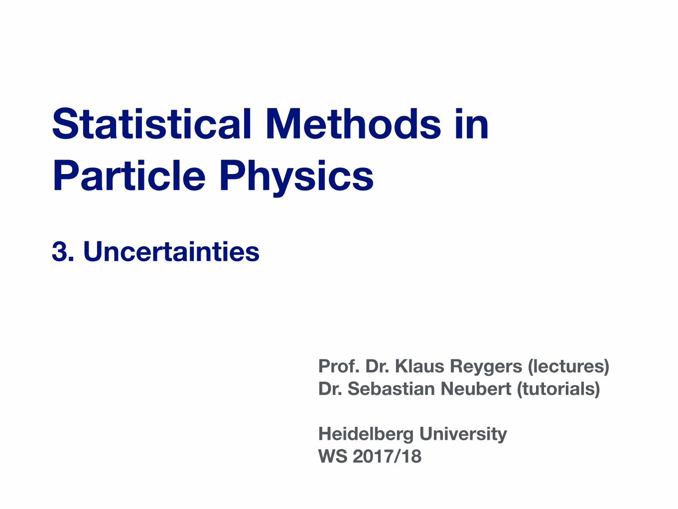
Precision and Accuracy

3


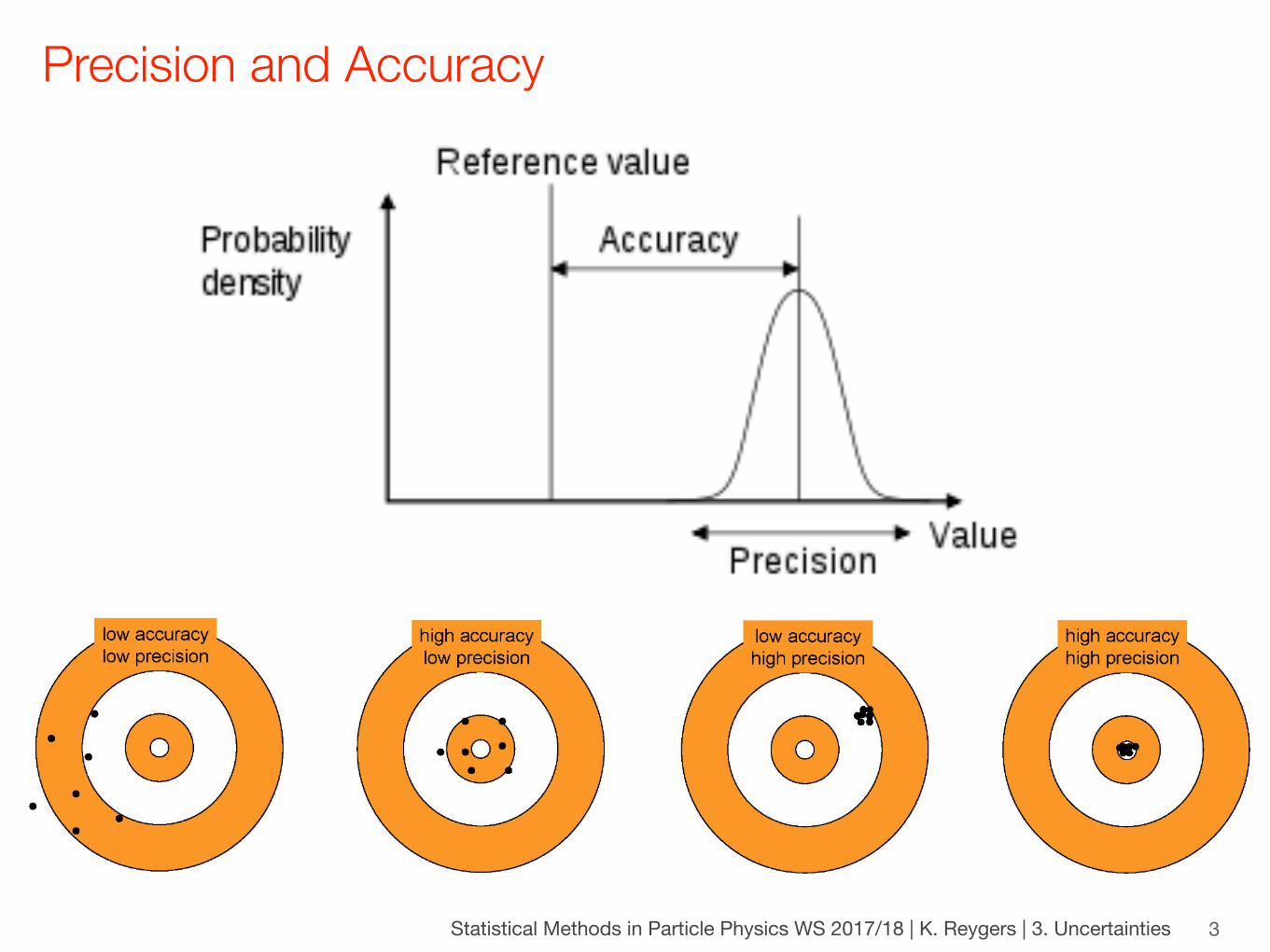
Ways to Quote Uncertainties

4

An uncertainty σ represents some kind of probability distribution(often a Gaussian, if not stated otherwise)

If no further information is given the interval x ± σ corresponds to a a probability of 68% ("1σ errors")


Statistical and Systematic Uncertainties

5

Statistical or random uncertainties ‣ Uncertainties that can be reliably estimated by repeating measurements ‣ They follow a known distribution like a Poisson rate or are determined empirically from

the distribution of an unbiased, sufficiently large sample. ‣ Relative uncertainty reduces as 1/√N where N is the sample size

Systematic uncertainties ‣ Cannot be calculated solely from sampling fluctuations ‣ In most cases don't reduce as 1/√N (but often also become smaller with larger N) ‣ Difficult to determine, in general less well known than the statistical uncertainty ‣ Systematic uncertainties ≠ mistakes

(a bug in your computer code is not a systematic uncertainty)

x = 2.34± 0.05 (stat.)± 0.03 (syst.)quoting stat. and syst. uncertainty separately gives us an idea whether taking more data would be helpful


Statistical Uncertainties: Examples

6

Radioactive decays (→ Poisson distribution) ‣ You measure N = 150 decays. ‣ The result is reports as N ± √N ≈ 150 ± 12

Efficiency of a detector (→ Binomial distribution) ‣ From N0 = 60 particles which traverse a detector, 45 are measured

‣ " = N/N0 = 0.75

�2N = N0"(1� ") �" =

s"(1� ")

N0=

r0.75 · 0.25

60= 0.06


Systematic Uncertainties: Examples

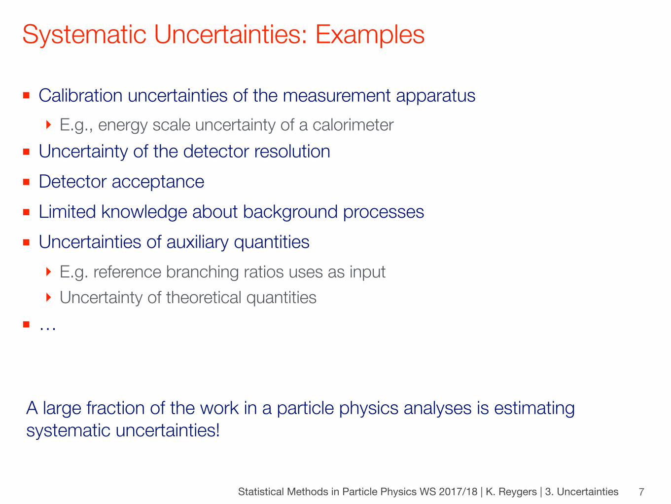
■ Calibration uncertainties of the measurement apparatus ‣ E.g., energy scale uncertainty of a calorimeter

■ Uncertainty of the detector resolution ■ Detector acceptance ■ Limited knowledge about background processes ■ Uncertainties of auxiliary quantities ‣ E.g. reference branching ratios uses as input ‣ Uncertainty of theoretical quantities

■ …

7

A large fraction of the work in a particle physics analyses is estimating systematic uncertainties!


How to Deal with Systematic Uncertainties?

8

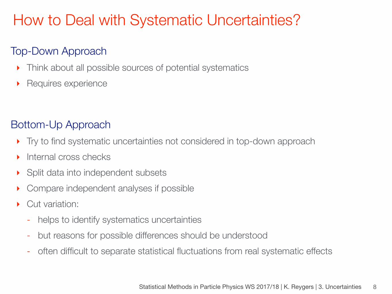
Top-Down Approach ‣ Think about all possible sources of potential systematics ‣ Requires experience

Bottom-Up Approach ‣ Try to find systematic uncertainties not considered in top-down approach ‣ Internal cross checks ‣ Split data into independent subsets ‣ Compare independent analyses if possible ‣ Cut variation:

- helps to identify systematics uncertainties - but reasons for possible differences should be understood - often difficult to separate statistical fluctuations from real systematic effects


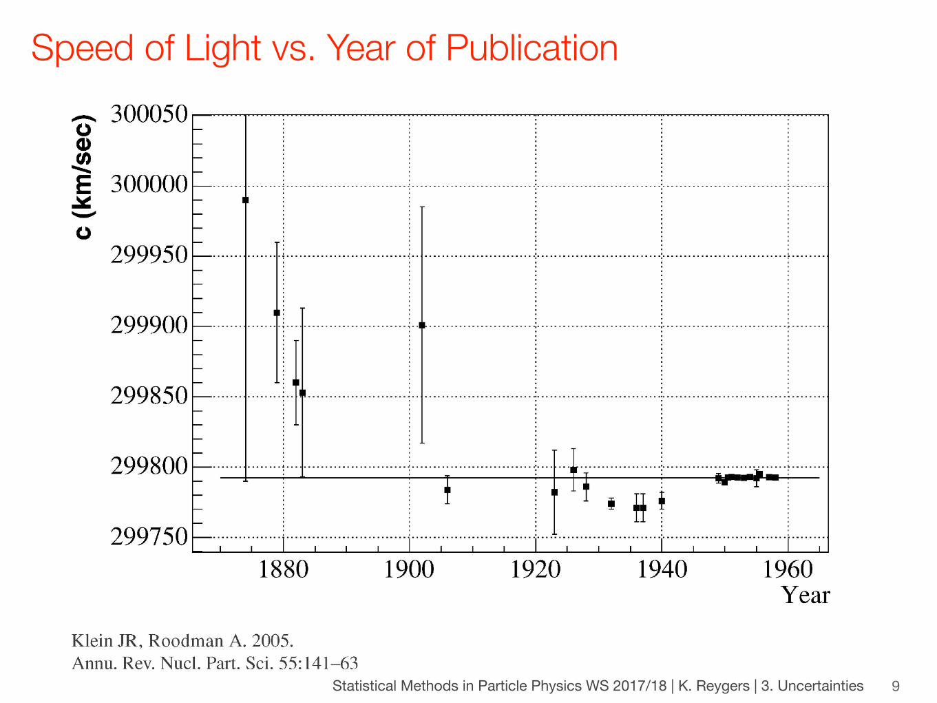
Speed of Light vs. Year of Publication

9


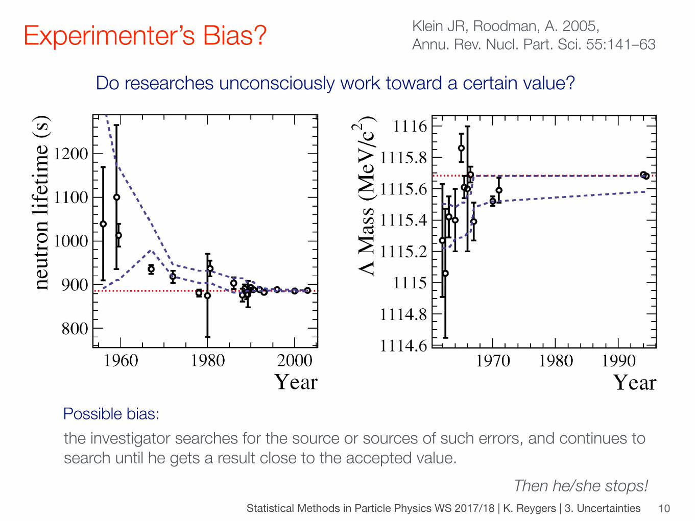
Experimenter’s Bias?

10

the investigator searches for the source or sources of such errors, and continues to search until he gets a result close to the accepted value.

Then he/she stops!

Klein JR, Roodman, A. 2005, Annu. Rev. Nucl. Part. Sci. 55:141–63

Possible bias:

Do researches unconsciously work toward a certain value?


Blind Analyses

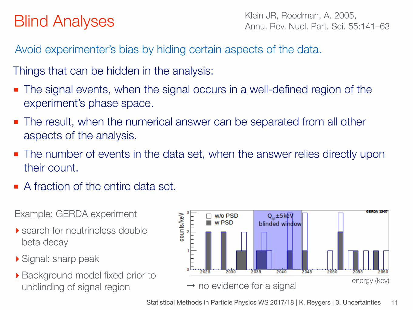
■ The signal events, when the signal occurs in a well-defined region of the experiment’s phase space.

■ The result, when the numerical answer can be separated from all other aspects of the analysis.

■ The number of events in the data set, when the answer relies directly upon their count.

■ A fraction of the entire data set.

11

Avoid experimenter’s bias by hiding certain aspects of the data.

Things that can be hidden in the analysis:

Unblinded spectrum

Cts in Qββ±5 keV golden silver BEGe totalexpected, w/o PSD 3.3 0.8 1.0 5.1observed, w/o PSD 5 1 1 7expected, w PSD 2.0 0.4 0.1 2.5observed, w PSD 2 1 0 3

Spectrum agrees with flat background expectation, no hint for gamma-line at Qββ !

W. Maneschg (MPI-K) GERDA: Results Phase I - Outlook Phase II Mainz, March 25, 2014 12 / 1

Example: GERDA experiment ‣ search for neutrinoless double

beta decay ‣ Signal: sharp peak ‣ Background model fixed prior to

unblinding of signal regionenergy (kev)→ no evidence for a signal

Klein JR, Roodman, A. 2005, Annu. Rev. Nucl. Part. Sci. 55:141–63


Combination of Systematic Uncertainties

12

In most cases one tries to find independent sources of systematic uncertainties. These independent uncertainties are therefore added in quadrature:

�2tot = �2

1 + �22 + ... + �2

n

Often a few source dominate the systematic uncertainty → No need to work to hard on correctly estimating the small uncertainties


Example: Neutral Pions Yields from Converted Photons in ALICE

13

photon conversion

e+

e-

e-

e+

γ1γ2

In this measurement the material budget uncertainty dominates the systematic uncertainty

⇡0 ! � + �, � +material ! e+ + e�


Describing Correlated Systematic Uncertainties (I)

14

Consider two measurement x1 and x2 with with individual random uncertainties σ1,r and σ2,r and a common systematic uncertainty σs:

xi = xtrue +�xi ,r +�xs

V [x2i ] = hx2i i � hxi i2

= h(xtrue +�xi ,r +�xs)2i � hxtrue +�xi ,r +�xsi2

= h(�xi ,r +�xs)2i

= �2i ,r + �2

s

Variance:

Covariance: cov[x1, x2] = hx1x2i � hx1ihx2i= ...

= �2s

h�xi ,ri = 0, h�xsi = 0,

h(�xi ,r)2i = �2

i ,r, h(�xs)2i = �2

s


Describing Correlated Systematic Uncertainties (II)

15

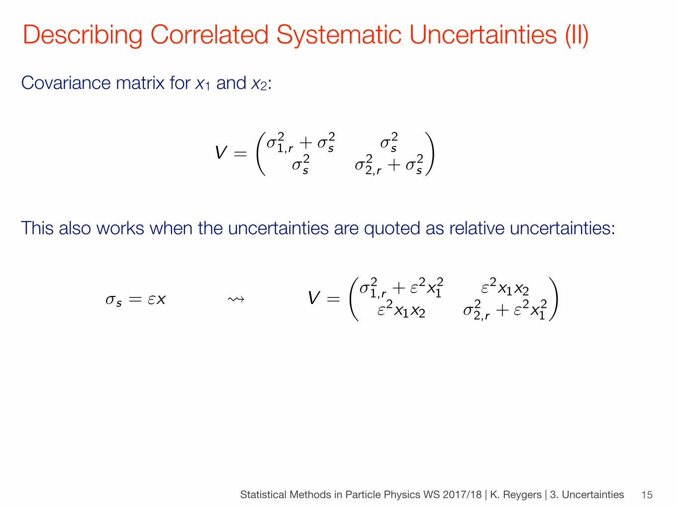
Covariance matrix for x1 and x2:

V =

✓�21,r + �2

s �2s

�2s �2

2,r + �2s

◆

This also works when the uncertainties are quoted as relative uncertainties:

�s = "x V =

✓�21,r + "2x21 "2x1x2"2x1x2 �2

2,r + "2x21

◆


Example:Transverse Momentum Spectrum of the Higgs-Boson

16

14 9 Results

[fb

/Ge

V]

H T/d

pfid

σd

0

0.2

0.4

0.6

0.8

1Data

Statistical uncertainty

Systematic uncertainty

Model dependence

ggH (POWHEGV2+JHUGen) + XH

ggH (HRes) + XH

XH = VBF + VH

(8 TeV)-119.4 fbCMS

[GeV]H

Tp

0 20 40 60 80 100 120 140 160 180 200Ra

tio t

o H

Re

s+X

H

0

1

2

3

Figure 4: Higgs boson production cross section as a function of pHT , after applying the unfold-

ing procedure. Data points are shown, together with statistical and systematic uncertainties.The vertical bars on the data points correspond to the sum in quadrature of the statistical andsystematic uncertainties. The model dependence uncertainty is also shown. The pink (andback-slashed filling) and green (and slashed filling) lines and areas represent the SM theo-retical estimates in which the acceptance of the dominant ggH contribution is modelled byHRES and POWHEG V2, respectively. The subdominant component of the signal is denoted asXH=VBF+VH and it is shown with the cross filled area separately. The bottom panel shows theratio of data and POWHEG V2 theoretical estimate to the HRES theoretical prediction.

To measure the inclusive cross section in the fiducial phase space, the differential measuredspectrum is integrated over p

HT . In order to compute the contributions of the bin uncertain-

ties of the differential spectrum to the inclusive uncertainty, error propagation is performedtaking into account the covariance matrix of the six signal strengths. For the extrapolation ofthis result to the fiducial phase space, the unfolding procedure is not needed, and the inclu-sive measurement has only to be corrected for the fiducial phase space selection efficiency efid.Dividing the measured number of events by the integrated luminosity and correcting for theoverall selection efficiency, which is estimated in simulation to be efid = 36.2%, the inclusivefiducial sB, sfid, is computed to be:

sfid = 39 ± 8 (stat) ± 9 (syst) fb, (4)

in agreement within the uncertainties with the theoretical estimate of 48 ± 8 fb, computed inte-grating the spectrum obtained with the POWHEG V2 program for the ggH process and includ-ing the XH contribution.

15

1.0 0.7 -0.2 -0.3 -0.2 -0.1

0.7 1.0 0.5 0.2 -0.0 -0.1

-0.2 0.5 1.0 0.8 0.4 0.2

-0.3 0.2 0.8 1.0 0.8 0.6

-0.2 -0.0 0.4 0.8 1.0 0.9

-0.1 -0.1 0.2 0.6 0.9 1.0

[GeV]H

Tp

[G

eV

]H T

p

Co

rre

latio

n

-1

-0.8

-0.6

-0.4

-0.2

0

0.2

0.4

0.6

0.8

1 (8 TeV)-119.4 fbCMS

[0,15] [15,45] [45,85] [85,125] [125,165] ]∞[165,[0

,15

][1

5,4

5]

[45

,85

][8

5,1

25

][1

25

,16

5]

]∞

[16

5,

Figure 5: Correlation matrix among the pHT bins of the differential spectrum.

10 SummaryThe cross section for Higgs boson production in pp collisions has been studied using theH ! W+W� decay mode, followed by leptonic decays of the W bosons to an oppositely chargedelectron-muon pair in the final state. Measurements have been performed using data from ppcollisions at a centre-of-mass energy of 8 TeV collected by the CMS experiment at the LHC andcorresponding to an integrated luminosity of 19.4 fb�1. The differential cross section has beenmeasured as a function of the Higgs boson transverse momentum in a fiducial phase space,defined to match the experimental kinematic acceptance. An unfolding procedure has beenused to extrapolate the measured results to the fiducial phase space and to correct for the de-tector effects. The measurements have been compared to SM theoretical estimations providedby the HRES and POWHEG V2 generators, showing good agreement within the experimentaluncertainties. The inclusive production sB in the fiducial phase space has been measured to be39 ± 8 (stat) ± 9 (syst) fb, consistent with the SM expectation.

AcknowledgmentsWe congratulate our colleagues in the CERN accelerator departments for the excellent perfor-mance of the LHC and thank the technical and administrative staffs at CERN and at other CMSinstitutes for their contributions to the success of the CMS effort. In addition, we gratefullyacknowledge the computing centres and personnel of the Worldwide LHC Computing Gridfor delivering so effectively the computing infrastructure essential to our analyses. Finally,we acknowledge the enduring support for the construction and operation of the LHC and theCMS detector provided by the following funding agencies: BMWFW and FWF (Austria); FNRSand FWO (Belgium); CNPq, CAPES, FAPERJ, and FAPESP (Brazil); MES (Bulgaria); CERN;CAS, MoST, and NSFC (China); COLCIENCIAS (Colombia); MSES and CSF (Croatia); RPF(Cyprus); SENESCYT (Ecuador); MoER, ERC IUT and ERDF (Estonia); Academy of Finland,MEC, and HIP (Finland); CEA and CNRS/IN2P3 (France); BMBF, DFG, and HGF (Germany);GSRT (Greece); OTKA and NIH (Hungary); DAE and DST (India); IPM (Iran); SFI (Ireland);INFN (Italy); MSIP and NRF (Republic of Korea); LAS (Lithuania); MOE and UM (Malaysia);

Correlation matrix of the pT bins:

⇢i ,j =Vi ,j

�i�j, V = covariance matrix

arXiv:1606.01522v1

Statistical Methods in Particle Physics WS 2017/18 | K. Reygers | 1. Basic Concepts 17

Error Propagation


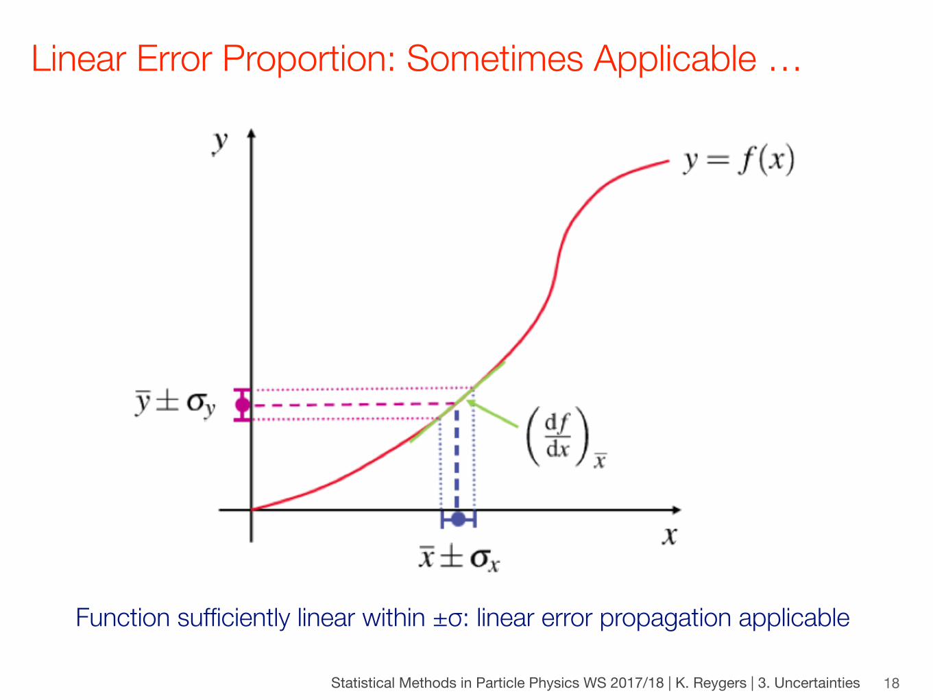
Linear Error Proportion: Sometimes Applicable …

18

Function sufficiently linear within ±σ: linear error propagation applicable


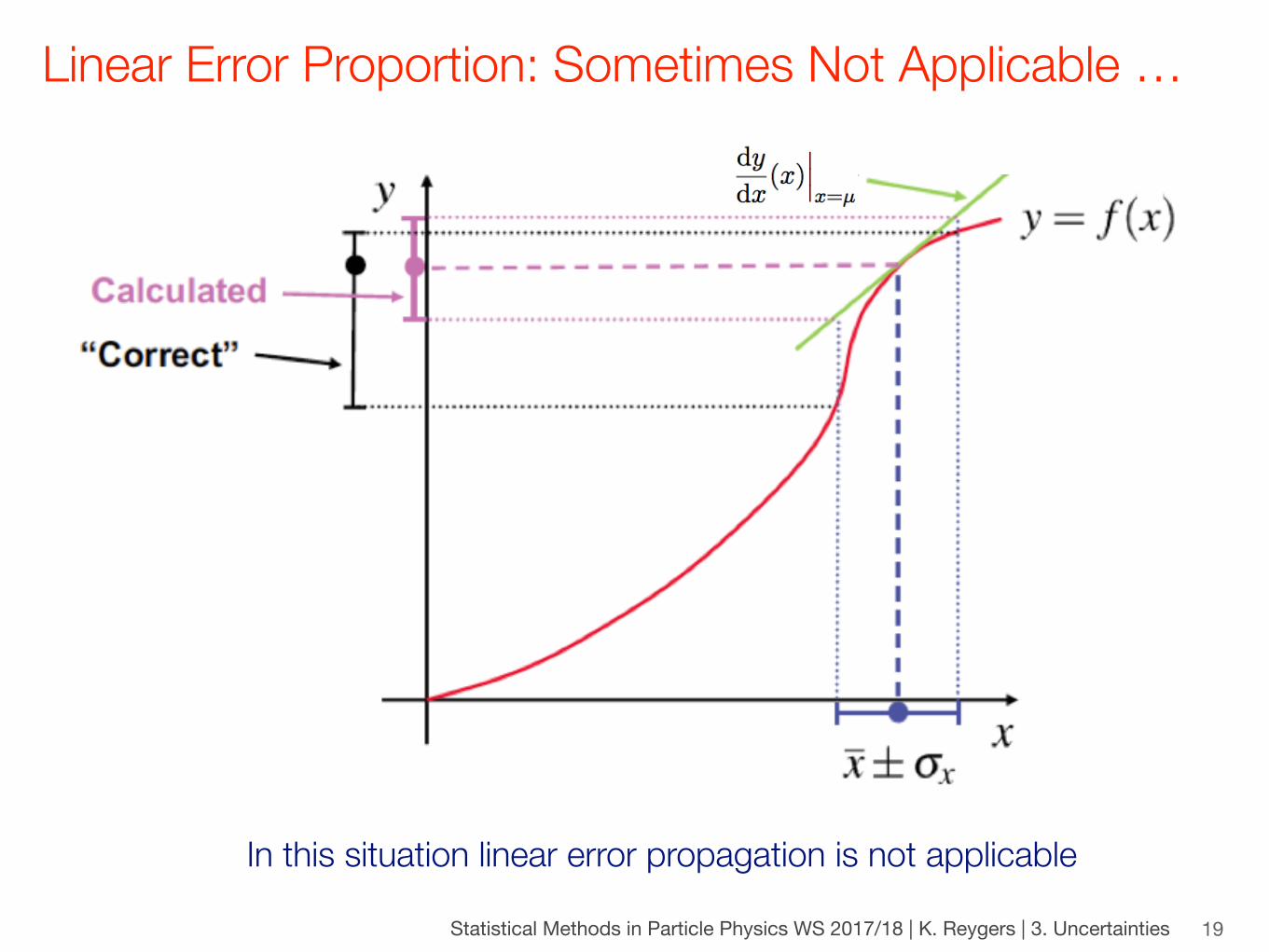
Linear Error Proportion: Sometimes Not Applicable …

19

In this situation linear error propagation is not applicable


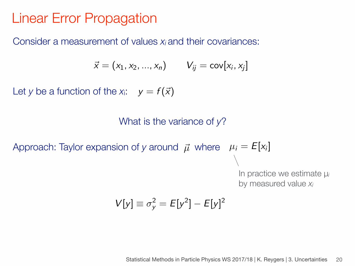
Linear Error Propagation

20

Consider a measurement of values xi and their covariances:

~x = (x1, x2, ..., xn) Vij = cov[xi , xj ]

Let y be a function of the xi: y = f (~x)

What is the variance of y?

Approach: Taylor expansion of y around where ~µ µi = E [xi ]

In practice we estimate μi by measured value xi

V [y ] ⌘ �2y = E [y2]� E [y ]2


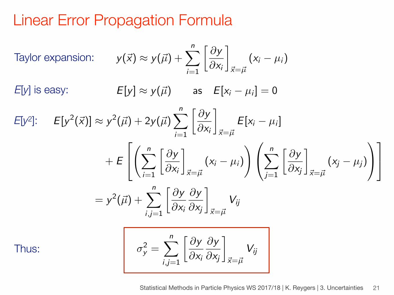
Linear Error Propagation Formula

21

y(~x) ⇡ y(~µ) +nX

i=1

@y

@xi

�

~x=~µ

(xi � µi )Taylor expansion:

E[y] is easy: E [y ] ⇡ y(~µ) as E [xi � µi ] = 0

E [y2(~x)] ⇡ y2(~µ) + 2y(~µ)nX

i=1

@y

@xi

�

~x=~µ

E [xi � µi ]

+ E

2

4

nX

i=1

@y

@xi

�

~x=~µ

(xi � µi )

!0

@nX

j=1

@y

@xj

�

~x=~µ

(xj � µj)

1

A

3

5

= y2(~µ) +nX

i ,j=1

@y

@xi

@y

@xj

�

~x=~µ

Vij

E[y2]:

Thus: �2y =

nX

i ,j=1

@y

@xi

@y

@xj

�

~x=~µ

Vij


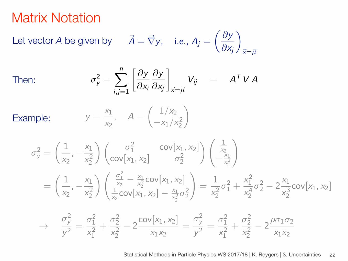
Matrix Notation

22

Let vector A be given by ~A = ~ry , i.e., Aj =

✓@y

@xj

◆

~x=~µ

�2y =

nX

i ,j=1

@y

@xi

@y

@xj

�

~x=~µ

Vij = ATV AThen:

y =x1x2

, A =

✓1/x2

�x1/x22

◆Example:

�2y =

✓1

x2,� x1

x22

◆✓�21 cov[x1, x2]

cov[x1, x2] �22

◆ 1x2

� x1x22

!

=

✓1

x2,� x1

x22

◆ �21

x2� x1

x22cov[x1, x2]

1x2cov[x1, x2]� x1

x22�22

!=

1

x22�21 +

x21x42

�22 � 2

x1x32

cov[x1, x2]

!�2y

y2=

�21

x21+

�22

x22� 2

cov[x1, x2]

x1x2=

�2y

y2=

�21

x21+

�22

x22� 2

⇢�1�2

x1x2


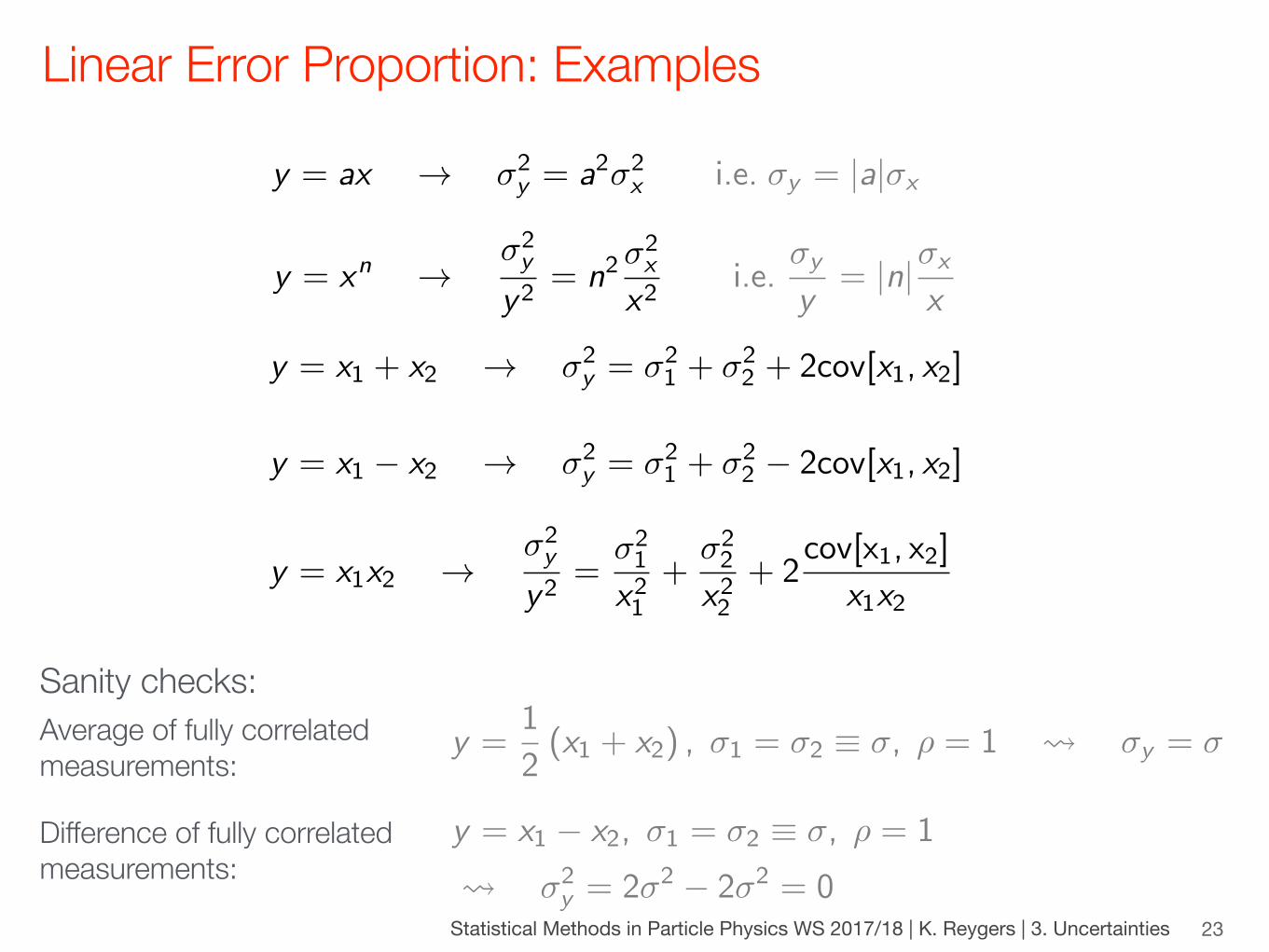
Linear Error Proportion: Examples

23

y = x1 + x2 ! �2y = �2

1 + �22 + 2cov[x1, x2]

y = x1x2 !�2y

y2=

�21

x21+

�22

x22+ 2

cov[x1, x2]

x1x2

y = xn !�2y

y2= n2

�2x

x2i.e.

�y

y= |n|�x

x

y = ax ! �2y = a2�2

x i.e. �y = |a|�x

Sanity checks:Average of fully correlated measurements:

y =1

2(x1 + x2) , �1 = �2 ⌘ �, ⇢ = 1 �y = �

Difference of fully correlated measurements:

y = x1 � x2, �1 = �2 ⌘ �, ⇢ = 1

�2y = 2�2 � 2�2 = 0

y = x1 � x2 ! �2y = �2

1 + �22 � 2cov[x1, x2]


Concrete Example: Momentum Resolution in Tracking

24

20

Momentum resolution

L

generally in experiment measure pt

multiple scattering term conts. in pt

track uncertainty ≈ pt

Charged particle moving in constant magnetic field:

pT/GeV = 0.3⇥ B/Tesla⇥ R/m

Measurements of space points yields Gaussian uncertainty for sagitta s which is related to pT as

R =L2

8s, pT = 0.3B

L2

8s

Momentum resolution:�pT

pT=

�s

s=

pT0.3BL2

�s

Important features: ‣ Relative momentum uncertainty

proportional to momentum ‣ Relative uncertainty prop. to uncertainty

of coordinate measurement

✓�pT

pT

◆2

= 0.0012 + (0.0005pT )2

Example:ATLAS nominal resolution

track uncertaintymultiple scattering


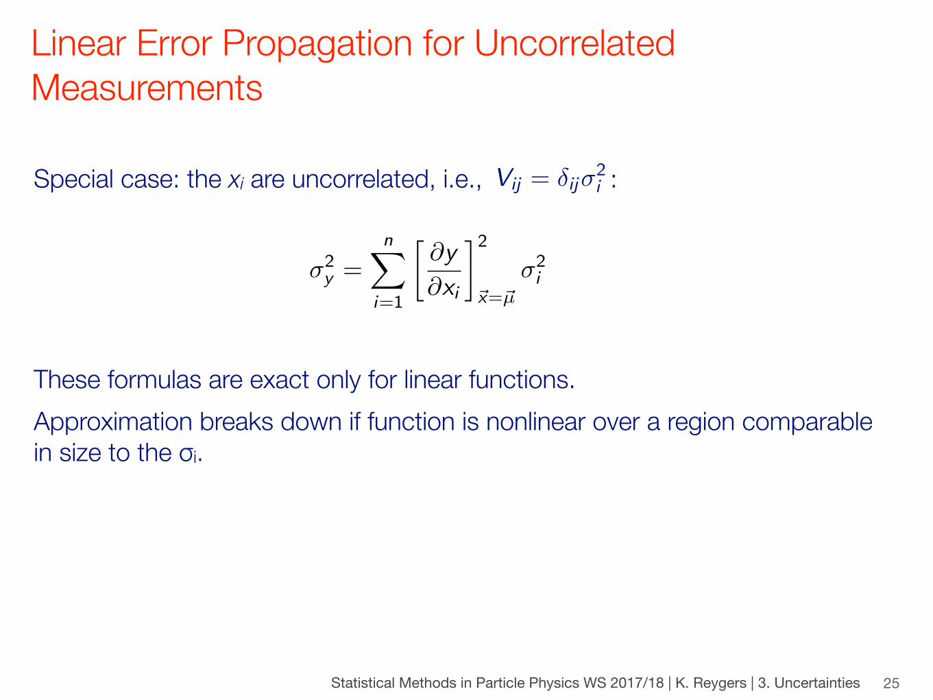
Linear Error Propagation for Uncorrelated Measurements

25

Special case: the xi are uncorrelated, i.e., : Vij = �ij�2i

�2y =

nX

i=1

@y

@xi

�2

~x=~µ

�2i

These formulas are exact only for linear functions. Approximation breaks down if function is nonlinear over a region comparable in size to the σi.


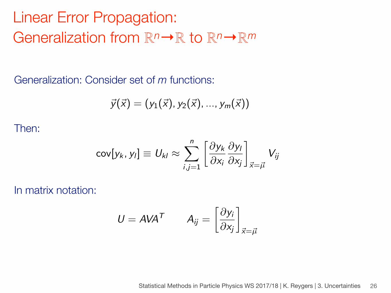
Linear Error Propagation: Generalization from ℝn→ℝ to ℝn→ℝm

26

Generalization: Consider set of m functions:

~y(~x) = (y1(~x), y2(~x), ..., ym(~x))

cov[yk , yl ] ⌘ Ukl ⇡nX

i ,j=1

@yk@xi

@yl@xj

�

~x=~µ

Vij

Then:

In matrix notation:

U = AVAT Aij =

@yi@xj

�

~x=~µ


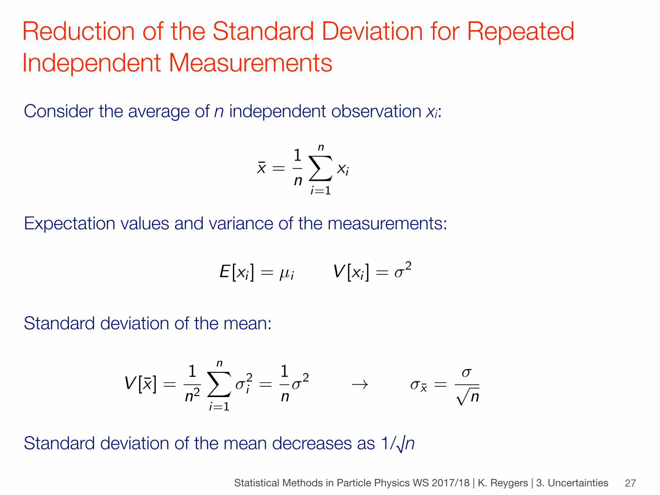
Reduction of the Standard Deviation for Repeated Independent Measurements

27

Consider the average of n independent observation xi:

x̄ =1

n

nX

i=1

xi

Expectation values and variance of the measurements:

E [xi ] = µi V [xi ] = �2

Standard deviation of the mean:

V [x̄ ] =1

n2

nX

i=1

�2i =

1

n�2 ! �x̄ =

�pn

Standard deviation of the mean decreases as 1/√n


Example: Photon Energy Measurements

28

The energy resolution of a γ-ray detector used to investigate a decaying nuclear isotope is 50 keV. ‣ If only one photon is detected the energy of the decay is known to 50 keV ‣ 100 collected decays: energy of the decay known to 5 keV ‣ To reach 1 keV one needs to observe 2500 decays


Averaging Uncorrelated Measurements

29

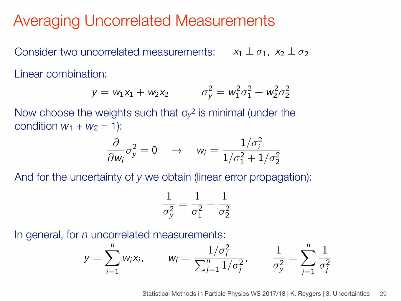
Consider two uncorrelated measurements:

Linear combination:

x1 ± �1, x2 ± �2

Now choose the weights such that σy2 is minimal (under the condition w1 + w2 = 1):

y = w1x1 + w2x2 �2y = w2

1�21 + w2

2�22

And for the uncertainty of y we obtain (linear error propagation):1

�2y=

1

�21

+1

�22

In general, for n uncorrelated measurements:

y =nX

i=1

wixi , wi =1/�2

iPnj=1 1/�

2j

,1

�2y=

nX

j=1

1

�2j

@

@wi�2y = 0 ! wi =

1/�2i

1/�21 + 1/�2

2


Example: Averaging Uncorrelated Measurements

30

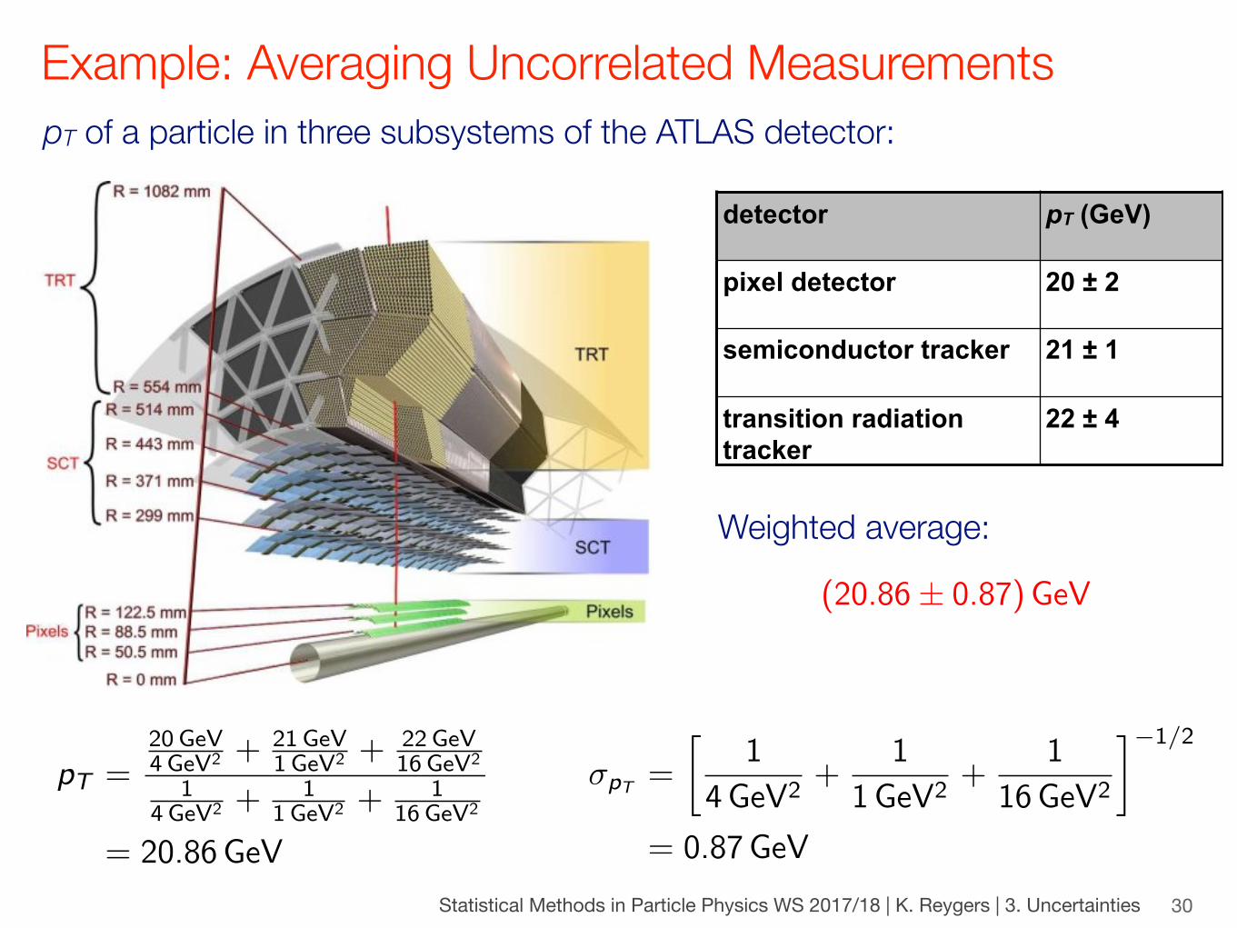
pT of a particle in three subsystems of the ATLAS detector:

detector pT (GeV)

pixel detector 20 ± 2

semiconductor tracker 21 ± 1

transition radiation tracker

22 ± 4

�pT =

1

4GeV2+

1

1GeV2+

1

16GeV2

��1/2

= 0.87GeV

pT =20 GeV4 GeV2 +

21 GeV1 GeV2 +

22 GeV16 GeV2

14 GeV2 +

11 GeV2 +

116 GeV2

= 20.86GeV

Weighted average:

(20.86± 0.87) GeV


Weighted Average from Bayesian Approach

31

Consider two measurements µ1 and µ2 with Gaussian uncertainties �1 and �2. In aBayesian approach the probability distribution for the true value x is given by

p(x) / L(µ1,µ2|x)⇡(x)

Assuming a flat prior ⇡(x) ⌘ 1 and independence of the two measurements oneobtains

p(x) / L(µ1|x)L(µ2|x)= G (µ1; x ,�1)G (µ2; x ,�2)

/ exp

�1

2

✓(x � µ1)2

�21

+(x � µ2)2

�22

◆�

The product of the two Gaussians gives a Gaussian with mean

µ = w1µ1 + w2µ2 where wi =1/�2

i

1/�21 + 1/�2

2

and standard deviation1

�2=

1

�21

+1

�22

→ same result as before


Monte Carlo Error Propagation

32

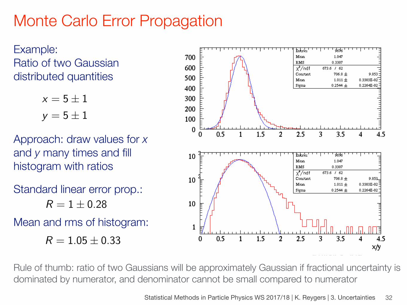
Example: Ratio of two Gaussian distributed quantities

Physics 509 25

Ratio of two Gaussians IVx = 5 ± 1 and y = 5 ± 1

Error propagation:R = 1 ± 0.28

Mean and RMS of R:1.05 ± 0.33

Gaussian fit to peak:1.01 ± 0.25

More non-Gaussian than first case, much better than second.

Rule of thumb: ratio of two Gaussians will be approximately Gaussian if fractional uncertainty is dominated by numerator, and denominator cannot be small compared to numerator.

x = 5± 1

y = 5± 1

Approach: draw values for x and y many times and fill histogram with ratios

Standard linear error prop.:R = 1± 0.28

Mean and rms of histogram:R = 1.05± 0.33

Rule of thumb: ratio of two Gaussians will be approximately Gaussian if fractional uncertainty is dominated by numerator, and denominator cannot be small compared to numerator

Statistical Methods in Particle Physicsreygers/... · Statistical Methods in Particle Physics WS...

Documents

Transcript of Statistical Methods in Particle Physicsreygers/... · Statistical Methods in Particle Physics WS...