Statistical Mechanics & Thermodynamics 2:Physical KineticsCompiled by Inon SharonySpring 2006-2008-2009

Class notes from the course by Professor Roman Mints1.1Prof. Mints's Homepagemints@post.tau.ac.ilO�ce adress: Shenkar (Physics) Building, Room 414O�ce phone: 9165

1

Contents1 Brownian Motion 51.1 Drunken Walk � The Random Walk as a Stochastic Process . . . . . . . . . . . . . . . . . . . . . 51.2 Probability Distribution . . . . . . . . . . . . . . . . . . . . . . . . . . . . . . . . . . . . . . . . . 51.3 Probability Distribution for Many Steps (Large N) on a Lattice . . . . . . . . . . . . . . . . . . . 51.4 Di�usion Equation . . . . . . . . . . . . . . . . . . . . . . . . . . . . . . . . . . . . . . . . . . . . 61.5 Di�usion Equation as a Continuity Equation . . . . . . . . . . . . . . . . . . . . . . . . . . . . . 62 Langevin Equation 92.1 One-Dimensional Ballistic Motion and Di�usion . . . . . . . . . . . . . . . . . . . . . . . . . . . . 92.2 Classical and Quantum Einstein Relations . . . . . . . . . . . . . . . . . . . . . . . . . . . . . . . 102.2.1 Ideal Classical Gas . . . . . . . . . . . . . . . . . . . . . . . . . . . . . . . . . . . . . . . . 112.2.2 Degenerate Fermion Gas (DEG) . . . . . . . . . . . . . . . . . . . . . . . . . . . . . . . . 112.3 Poiseuille Flow . . . . . . . . . . . . . . . . . . . . . . . . . . . . . . . . . . . . . . . . . . . . . . 152.4 Di�usion in Ambipolar Plasma . . . . . . . . . . . . . . . . . . . . . . . . . . . . . . . . . . . . . 162.5 Debye-Hückel Screening (1923) . . . . . . . . . . . . . . . . . . . . . . . . . . . . . . . . . . . . . 172.5.1 The Screening Length ��1 in Di�erent Materials . . . . . . . . . . . . . . . . . . . . . . . 173 Self Heating Phenomena 193.1 Heat Di�usion Equation . . . . . . . . . . . . . . . . . . . . . . . . . . . . . . . . . . . . . . . . . 193.2 Nonlinear Stationary States . . . . . . . . . . . . . . . . . . . . . . . . . . . . . . . . . . . . . . . 243.2.1 Current Carrying Superconducting Wire . . . . . . . . . . . . . . . . . . . . . . . . . . . . 243.2.2 Chemical Reactions on the Surface of a Catalyst . . . . . . . . . . . . . . . . . . . . . . . 273.2.3 Metal - Dielectric Phase Transition . . . . . . . . . . . . . . . . . . . . . . . . . . . . . . . 273.3 Linear Stability of Nonlinear Stationary States . . . . . . . . . . . . . . . . . . . . . . . . . . . . 283.4 Propagation of Single Nonlinear �Switching� Waves . . . . . . . . . . . . . . . . . . . . . . . . . 314 Di�usion in Momentum-Space 364.1 Electron-Phonon Collisions in Metals at Low Temperatures . . . . . . . . . . . . . . . . . . . . . 364.2 Relaxation of Heavy Particles in a Gas of Light Particles . . . . . . . . . . . . . . . . . . . . . . . 374.3 Fokker-Planck Equation . . . . . . . . . . . . . . . . . . . . . . . . . . . . . . . . . . . . . . . . . 375 Boltzmann Equation 415.1 Liouville's theorem . . . . . . . . . . . . . . . . . . . . . . . . . . . . . . . . . . . . . . . . . . . . 415.2 Boltzmann equation . . . . . . . . . . . . . . . . . . . . . . . . . . . . . . . . . . . . . . . . . . . 425.3 collision integral . . . . . . . . . . . . . . . . . . . . . . . . . . . . . . . . . . . . . . . . . . . . . 425.4 � -approximation . . . . . . . . . . . . . . . . . . . . . . . . . . . . . . . . . . . . . . . . . . . . . 425.5 heat conductivity and viscosity of gases . . . . . . . . . . . . . . . . . . . . . . . . . . . . . . . . 436 Kinetics of a Degenerate Electron Gas 496.1 Electrical and thermal conductivities . . . . . . . . . . . . . . . . . . . . . . . . . . . . . . . . . . 496.2 Wiedemann-Franz law . . . . . . . . . . . . . . . . . . . . . . . . . . . . . . . . . . . . . . . . 516.3 Skin-e�ect . . . . . . . . . . . . . . . . . . . . . . . . . . . . . . . . . . . . . . . . . . . . . . . . . 526.4 Electrical Conductivity in a Magnetic Field . . . . . . . . . . . . . . . . . . . . . . . . . . . . . . 566.5 Onsager relations . . . . . . . . . . . . . . . . . . . . . . . . . . . . . . . . . . . . . . . . . . . . 626.6 Thermo-Electrical Phenomena . . . . . . . . . . . . . . . . . . . . . . . . . . . . . . . . . . . . . . 637 Master Equation 667.1 Magnetic resonance . . . . . . . . . . . . . . . . . . . . . . . . . . . . . . . . . . . . . . . . . . . . 687.2 Överhauser e�ect . . . . . . . . . . . . . . . . . . . . . . . . . . . . . . . . . . . . . . . . . . . . 69

2

8 Fluctuation-Dissipation Theorem 718.1 Harmonic analyses of Langevin equation . . . . . . . . . . . . . . . . . . . . . . . . . . . . . . . 718.2 velocity-velocity and force-force correlation functions . . . . . . . . . . . . . . . . . . . . . . . . . 718.3 power spectra . . . . . . . . . . . . . . . . . . . . . . . . . . . . . . . . . . . . . . . . . . . . . . . 718.4 classical and quantum limits . . . . . . . . . . . . . . . . . . . . . . . . . . . . . . . . . . . . . . . 758.5 Nyquist formulas. . . . . . . . . . . . . . . . . . . . . . . . . . . . . . . . . . . . . . . . . . . . . . 759 Damping in Collisionless Plasma 769.1 Self-consistent �eld and collision-less approximations . . . . . . . . . . . . . . . . . . . . . . . . . 769.2 Vlasov equations . . . . . . . . . . . . . . . . . . . . . . . . . . . . . . . . . . . . . . . . . . . . 769.3 plasma waves . . . . . . . . . . . . . . . . . . . . . . . . . . . . . . . . . . . . . . . . . . . . . . . 789.4 Langmuir plasma frequency . . . . . . . . . . . . . . . . . . . . . . . . . . . . . . . . . . . . . . 799.5 Landau damping . . . . . . . . . . . . . . . . . . . . . . . . . . . . . . . . . . . . . . . . . . . . . 80

3

Di�usion

4

1 Brownian Motion1.1 Drunken Walk � The Random Walk as a Stochastic ProcessA particle moving in one dimension, with probability p to take a step in the right direction during any giventime-step, and q to take a step in the left direction. The step length is a.m steps are made in the right direction and n steps are made in the left direction. Many steps are taken, sothat m+ n � N � 1.1.2 Probability DistributionWhat is the probability that such a course is taken (de�ned by m and n)?

W (m;n) � pmqn N !n!m! �� Nn � pmqnNX

n=0� Nn � pN�nqn = (p+ q)N = 1N = 1

Where in the second line we used the expansion for the Newton binomial.1.3 Probability Distribution for Many Steps (Large N) on a LatticeThe average number of steps right can be designated �m � pN , and likewise to the left �n � qN . We can writem = �m+ xn = �n� xWhere x is the deviation from the average number of steps. We can also de�ne the total deviation as ` �N (p� q) + 2x.Assuming x� �n = qN = (1� p)N and also x� �m = pN , we will look at

W 0@qN � x| {z }n ; pN + x| {z }m1A = qqN�xppN+x � N !(qN � x)! (pN + x)!

Using the Stirling formula ln (N !) = N � �ln (N)� 1 +O � 1N ��lnW (n;m) = n ln q +m ln p+ ln (N !)� ln (n!)� ln (m!)' n ln q +m ln p+N lnN �N � n lnn+ n�m lnm+mlnn = ln (qN � x)

= ln�qN �1� xqN ��= ln (qN) + ln�1� xqN �= ln (qN)� xqN � 12

� xqN �2 +O "� xqN �3#

And similarly for the expression lnm. In all we can sum up all the quadratic terms in x, and get the coe�cientsfrom normalization lnW (n;m) ' � x22N �1p + 1q� = � x22pqNW (n;m) / e� x22pqNW (n;m) = 1p2�pqN e� x22pqN

5

�x � hxi = 0�x2 � x2� = pqNphx2i / pN�� h`i = (p� q)N�2 � `2� = (p� q)2N2 � 4pqNNote that all the results except � are symmetric in the switch p$ q.If p 6= q, there will be a constant drift of (p� q)2N2. For a symmetric random walk (p = q),�2 = Np �2 = pNWe de�ne the total deviation length L � ` � a , and total di�usion time t � N � � , so that

�L2 = �2 � a2 = N � a2 = t� � a2 = 2 � a22� � t � 2 � D � tp �L2 / ptWhere D � a22� is the de�ned di�usion constant, or di�usivity.1.4 Di�usion EquationThe number of particles at point x on a lattice (of step size a) at time t (in discrete time-steps of length �) isdependent on the amount of particles which occupied the sites to the left and right of x at the previous time-step, and on the number of particles which may be created or annihilated at x during the current time-step,which can be described by a source/sink rate function f (x; t):n (x; t) = q � n (x+ a; t� �) + p � n (x� a; t� �) + f (x; t) � � (1)We expand the n terms in series (simultaneously to second order in x and �rst order in t)

n (x� a; t� �) ' n (x; t� �)� a � @n (�; t� �)@� j�=x + 12a2 � @2n (�; t� �)@�2 j�=x � � � @n (x� a; s)@s js=tSubstituting back in 1

n (x; t) ' n (x; t) + (q � p) � a � @n (x; t)@x + 12a2 � @2n (x; t)@x2 � � � @n (x; t)@t + � � f (x; t)@n@t = q � p� � a| {z }��v �@n@x + a22�|{z}D �@2n@x2 + f@n@t = ��v @n@x +D@2n@x2 + f

The resultant di�usion equation can be viewed as a continuity equation.1.5 Di�usion Equation as a Continuity Equation@n@t + @j@x = 0In order for the di�usion equation to be a continuity equation, the current must be de�ned as

j � �vn�D@n@x6

Disregarding the external function f (x; t) for now, we have@n@t = ��v @n@x +D@2n@x2Moving to a reference frame which is moving at velocity �v, i.e. de�ning n � n (x� �vt; t)@n@t = D@2n@2xWhich is a simple di�usion equation.As an example, we add point Dirichlet initial conditions. The result can serve as a Green's function forany general initial condition we may wish to apply later.@n@t = D@2n@x2 + � (t) � (x)The solution is gotten by taking the Fourier transform of both sides of the equation

n (x; t) = 1p4�Dte� x24DtIn general, for any linear equation we will come across, we will try to solve using a Fourier transform.di�usion with Initial ConditionA gas with uniform density n0 occupies a semi-in�nite space, and is held behind an in�nite-planar partition atx = 0. At t = 0 the partition is removed. What is the time-dependent gas density, n (t)?We will solve the 1-D di�usion equation with the boundary condition for an initial point concentration atx = 0. Then we will use this solution to integrate over all contributions from �1 � x0 � 0.@n@t = D@2n@x2 + � (t) � (x)n0Using a Fourier transformZ 1�1 dte�i!t Z 1�1 dxe�ikx @n@t = Z 1�1 dte�i!t Z 1�1 dxe�ikx �D@2n@x2 + � (t) � (x)n0�i!n (k; !) = �Dk2n (k; !) + n0n (k; !) = n0Dk2 + i!n (x; t) = 1(2�)2 Z 1�1 dtei!t Z 1�1 dxeikxn (k; !)

= n0p4�Dte�x2=4Dtn (x; t) = Z 0�1 n (x0; t) dx0

= Z 0�1 n0p4�Dte�(x�x0)2=4Dtdx0� Z 1

xp4Dtn0p� e�z2dz

z � x� x0p4Dtn (x; t) = n02 �1� erf � xp4Dt

��The complimentary problem deals with an initial density n0 behind some partition, which is lifted at t = 0.What is the density as a function n (t) of time on the originally vacant side of the partition?

7

di�usion with Boundary ConditionA particle starting at x0 is di�using along the x-axis. A sticky wall is placed at x = 0. What is the probabilityfor the particle to get stuck as a function of t?The equation to be solved is (di�usion equation with point initial condition n (x0; 0) = 1)@n@t = D@2n@x2 + � (t) � (x� x0)with the boundary condition n (0; t) = 0for all t.In analogy to electrostatics, the boundary condition can be mathematically represented using the �methodof mirror charges�, i.e. a mirror particle with density �n0 which begins di�using at time zero at �x0. Thesolution is the sum of the �real� (n0) and �mirror� (�n0) particlesn (x; t) = n0 (x� x0; t)� n0 (x+ x0; t)Where each of the �real� or �mirror� particles has a solution of the form of di�usion without the boundarycondition

n0 (x� x0; t) = 1p4�Dte�(x�x0)2=4DtThe �ux at the boundary isj (0; t) = �D@n (x; t)@x jx=0

= 2D@n0 (x; t)@x jx=0= x02p�D � t�3=2 � e�x20=4Dt

The probability to get stuck is P (t) = Z t0 dt0j (0; t0)The complete solution requires numeric integration.An alternate route is to compute 1� P (t) = R10 n (x; t) dx, i.e., via the probability that the particle is notstuck at time t.

8

2 Langevin EquationWe would like to write equations of motion for a particle (of gas for instance, and of radius R) moving ina viscous environment (another gas, for instance, with viscosity coe�cient �). Starting from the Newtonequation we write m _~v = ~F (t; v) � ~f (~v) + ~F (t)~f (~v) = ��~v� = 6��RWhere ~f is a friction force and ~F is a random force, and the friction coe�cient � is related to the viscosityof the environment � according to the Stokes relation (given here for a spherical geometry).2.1 One-Dimensional Ballistic Motion and Di�usion2In one dimension m�x (t) = �� _x (t) + F (t)multiplying by x (t) we getm2 d2dt2 �x2 (t)��m � ddtx (t)�2 = ��2 ddt �x2 (t)�+ F (t)x (t)Suppose the time between collisions is � and we average over times su�ciently longer than � .hF (t)x (t)i = hF (t)i hx (t)i = 0 � 0Since the random force is uncorrelated to the particle trajectory, and both have zero mean. Therefore the lastterm on the RHS is zero.From di�usion, y (t) � 12 x2 (t)� = Dt, so m2 d2dt2 x2 (t)� = 0. Therefore the �rst term on the LHS is zero.The kinetic energy of the particle is m2 D� ddtx (t)��2E = 12kBT .The �rst term on the RHS is ��2 ddt x2 (t)� = ��D.In all �kBT = ��DD = kBT� � BkBTWhere B � ��1 is named the mobility, �rst implied by Galileo, and see also 2.2.Example:A particle of radius 0:5�m is solvated in water at 20�C which has viscosity 0:01 with the appropriatecgs units. The particle time dependent RMS displacement isr2 (t)� = x2 (t)�+ y2 (t)�+ z2 (t)� = 3 � 2Dtphr2 (t)i = p6Dt =r6kBT� tphr2 (40 s)i ' 10�mBack to the general problem,

y (t) � 12 x2 (t)�m�y (t)�m _x2 (t)�| {z }kBT = �� _y (t)m�y + � _y = kBT2Appeared in 2006A and 2007B.

9

The exact solution to this equation is (with initial conditions y (0) = _y (0) = 0)y (t) = kBT� ht� m� �1� e��t=m�i

which leads to de�ne the time scale t0 � m� . For long times, i.e. t� t0 the exponent falls andy (t) ' kBT� � t = Dt

so at long times we recover simple di�usion-like behavior. At short times, i.e. t� t0 we expand the exponentto second order in tt0 (all previous orders cancel out) andy (t) ' kBTm � t2

which corresponds to ballistic motion.An assessment for the value of t0 for a sphere ist0 = m� = 4�R3�6��R / ��R2

For the values of the intrinsic properties of water (�; �) and a particle radius of 0:5�m we get t0 ' 2� 10�8 s =20ns. This is a very short relaxation time, which means that experiment will show only the di�usive behavior.2.2 Classical and Quantum Einstein RelationsRecall the relations D = kBT� = BkBT .Particles performing overdamped motion have a very short mean free path, i.e. the time between collisionsis much shorter than any other interesting timescale in the system.Assume particles distributed with density n (~r) acted upon by a friction force ~f = �~v = 1B~v, but no randomforce. m _~v � ~f~v = B ~fThe particle current is composed of an external force / potential term, and a concentration gradient term~j = n~v �D~r � n= nB ~f �D~r � n= �nB~r � V �D~r � nwhere V (~r) is a potential from which the force ~f is derived.In equilibrium, ~j = 0. Also, in equilibrium � (~r) + V (~r) = const: (here � (~r) is the chemical potential).~r � V = �~r � �= �@�@n ~r � nWhere the second line was gotten using the chain rule. Substituting back we have

0 = nB@�@n ~r � n�D~r � nD = nB@�@nThis is the Einstein relation in its most general form.Particular examples:10

2.2.1 Ideal Classical GasFrom combinatorics we have the dependence of � (n). The dependence on temperature is given from theSackur-Tetrode formula.� (n; T ) = kBT lnn+ � (T )@�@n = kBTnD = nBkBTn = BkBT (2)

2.2.2 Degenerate Fermion Gas (DEG)The dependence of the Fermion gas on the density is given, to �rst order, by the density dependence of theFermi energy (eqn. 6).� ' "F (n) +O "�kBT"F

�2#"3�DF (n) / n2=3@�@n = 23 "FnD = nB 23 "Fn = 23B"F

Size of a Puddle of Falling DropsDrops falling under g = 9:8ms�2 from a height h = 1m di�use in the horizontal plain as they fall. What is theRMS radius of the resulting puddle, r2�? Compare this with the drop size, R. Assume the drops have massm = 10�10 g and density � = 0:9 g cm�3, and that the air is at temperature T = 300K.r2� = x2 + y2� = 2 � 2Dt = 4kBT� t� = 6��Rm = 4�R33 �R = � 3m4���1=3Solving the Langevin equation for the vertical motion:

_vz = � �mvz + g_vz + �mvz = gddt �vz (t) � e �m t� = ge �m t

vz (t) � e �m t � vz (0) = Z t0 ge �m t0dt0vz (t) � e �m t = mg� �e �m t � 1�vz (t) = mg� �1� e� �m t�

The vertical motion is characterized by the time scale�0 � m� / mm1=3 = m2=3 � 111

Meaning that this time scale is much less than the time scale for free particle motion, characterized by mv22 / m.Therefore the transient e�ect in the result for vz (t) can be disregardedvz (t) ' mg� = Bmg

And the time that the drops take to fall is t = hvz = h�mg .Putting it all together, r2� = 4kBT6 � � h 6 �mg = 4hkBTmg� 4 � 1m � 1:380� 10�23 J K�1 � 300K10�13 kg � 9:8ms�2' 1:689� 10�8mphr2i � 1:3� 10�4m

R � � 3 � 10�10 g4� � 0:9 g cm�3�1=3' 3� 10�4 cm = 3� 10�6mSince the puddle size, phr2i, is two orders of magnitude greater than the single drop size, R, the e�ect shouldbe measureable. The puddle size is also independent on the internal composision of the drops, which wouldmanifest in the dorp mobility, B, which does not appear in the �nal result.Gas Escaping from a Box to a VacuumAn atomic gas has density n (t) satisfying n (t = 0) � n0. The gas occupies a box of volume V and hastemperature T . The gas particles' mass is m, and it escapes through a hole in the box of area A. How muchheat needs to be supplied externally to keep the box at a constant temperature?The velocity distribution:

f~v = � m2�kBT�3=2 exp �� m2kBT �v2x + v2y + v2z��

For a spherically symmetric distribution:fv = 4�v2� m2�kBT

�2=3 exp �� mv22kBT�

the average velocity is�v � hvi = Z 10 fvvdv = 12

Z 10 fvd �v2�= 4�� m2�kBT

�2=3�2kBTm �2 Z 10 te�tdt= 2��3=2

r2kBTm= r8kBT�mWe are interested only in the velocities which contribute to a particle leaving the box, i.e. velocities with a

12

positive component along the x-axis (where the x-axis is perpendicular to the hole in the box).�v+x = Z 10 vxr m2�kBT e� mv2x2kBT dvx= 12

Z 10r m2�kBT e� mv2x2kBT d �v2x�

= 12Z 10

r2kBT�m e�tdt= rkBT2�m= 14�vWe next write the continuity equation for the number of particles in the box, N (t) = V � n (t), where (at lowgas densities) we assume that the current of particles leaving the box through the hole can be approximated aslinearly dependent on the local particle density near the hole:ddtN (t) = V ddtn (t) = �A � n (t) � �v+x

= �A � n (t) � 14 �vThe solution is an exponential decrease:n (t) = n0 � e�A�v4V �t = n0 � e�t=�� � 4VA�vThe leaving energy �uxh"�i = h"v+x iv+x � = 2kBT

Each atom has a thermal kinetic energy of 32kBT , which is smaller than the outgoing energy �ux per particle.The box is cooled because the slow particles leave more slowly than the fast particles (the reason for this is thelack of correlation between di�erent particles). To keep the temperature constant, the incoming heat �ux needsto cancel the outgoing energy taken away with the leaving particles.~P = ddtEk (t)= �12kBT � ddtN (t)= �12kBTV � ddtn (t)= 12kBTV � A�v4V � n (t)= kBTA�vn08 e�A�vt4V= kBT2 N0� e�t=�The total energy supplied up to time t is

Q (t) = Z t0 dt0P (t0)= 32kBTV � A�v4V � Z t0 dt0n (t0)= 32kBTV n0 h1� e�A�vt04V i= 32N0kBT h1� e�A�vt04V i

13

Corollary A similar problem could be where the gas escapes not to a vacuum, but to a surrounding with �xedpressure and temperature, i.e. �xed outside particle concentration nout. The solution is gotten by computingthe �ux of particles from outside the box into it, and writing the continuity equation in terms of the sum of two�uxes: outgoing and incoming. When the temperature inside and outside the box are equal, the terms A and�v appear equally in both �uxes, and the derivative of n (t) is a function of nout � n.ddtN (t) = V ddtn (t) = Jout + Jin= �A � n (t) � �v+x +A � nout � �v�x= �A � [nout � n (t)] � 14 �vWhere the last line is valid if �v�x = �v+x , i.e. when the temperature is equal inside and outside the boxddtn (t) = nout � n�� � A�v4VSolution to the non-homogenous �rst-order ODE_n (t) + 1� n (t) = 1� noutddt hn (t) � et=�i = 1� noutet=�n (t) � et=� � n0 = Z t0 1� noutet0=�dt0n (t) � et=� = n0 + nout het=� � 1in (t) = n0e�t=� + nout h1� e�t=�i

Knudsen's Law3Two containers of volumes V1 and V2 are connected through a small hole of area A. The containers are held ata separate temperatures T1 and T2, respectively, and we assume that these temperatures remain constant forthe times relevant in the question. What is the ratio of pressures, P1 and P2, respectively, which are created inthe containers?If the hole size scale L � pA is much larger than the mean free path of the particles, `, then there willbe particle-particle collisions near the hole, and the pressures on both sides of the hole will equilibrate quickly,such that P1 = P2. When we say �the hole is small�, what is meant is ` � L. In order to increase the meanfree path, `, we can use a very sparce gas. In this case the pressures equalize much more slowly, and for shorttimes we can write P1P2 = N1RT1N2RT2 � V2V1 = N1T1V2N2T2V1 = n1T1n2T2we require that at equilibrium the change in the number of particles in any one of the containers has to be zero.This change is caused by a current of leaving particles and a current of entering particles, through the hole

0 = ddtN1 = V1 ddtn1 (t) = J2!1 (t)� J1!2 (t)J1!2 (t) = J2!1 (t)n1 (t) � �v1 = n2 (t) � �v2n1 (t) �pT1 = n2 (t) �pT2n1n2 = rT2T13Appeared in 2006B.14

so that in all, P1P2 =rT1T22.3 Poiseuille Flow4We are interested in the outgoing �ux of a gas escaping from a box to a vacuum through a narrow cylindricaltube of length L.We assume that the gas density is low in the sense that the mean free path, `, is much greater than thecylinder radius, R. This means that gas leaving the box via the tube experiences collisions only with the cylinderwalls5, and not with other gas particles.We also assume that the escape process is so slow that the gas density in the box is nearly unchanged, andremains n0 throughout the process. That is, we are only interested in short enough time scales, such that n0does not change in the time we concern ourselves with.The particle �ux is de�ned as j = �D @n@x . The di�usion coe�cient is given in terms of the RMS velocity

D = 12 a2� = 12a�v (T )�v2 � v2� = kBTmThe characteristic length, a, is taken as R. D = 12R�vThe particle concentration gradient, @n@x is estimated as linear in the tube, for lack of better knowledge.

j = �D � 0� n0L= 12R�v � n0LThe particle current through the tube is J = A � j= �R2 � 12R�v � n0L= �2 � n0�vL �R3 / R3The prefactors are rarely exact, the functional dependence is what's important because it is easily veri�edthrough experiment.Another approach: Large n0The pressure in the box is p0 = n0kBT , and the pressure outside it is zero (vacuum).The gas viscosity is � = 13`nm�v = 13nm�v2�where the last equality is due to ` � �v� . This case was solved by Poisseuille in 1840

J = �n2kBTR48�L / R4� / R4`if we increase the average density of particles in the tube, the mean free path will decrease until it reaches theorder of R and then we will recover J / R3:If we were to take `� R, the result would be J / R4.4Appeared in 2007A.5We ignore ballistic transport, in which a gas particle can travel the entire length of the cylinder without hitting anything.15

Contribution from Ballistic TransportExcept for the current which comes from di�usion, there is a contribution from the current of ballisticly movingparticles (i.e., no collisions with tube or other particles, from box to vacuum).The particles that can move through the tube without colliding with the tube walls are only those whichhave a velocity nearly parallel to the tube itself. This angle is � RL small. The RMS speed of these particles is�v, and the �ux due to their contribution is j � n � RL � �v. This is the same contribution as the one we got fromdi�usion, so the dependence on R remains the same, J / R3 (only with a di�erent coe�cient).2.4 Di�usion in Ambipolar Plasma6We regard a plasma (ionized gas) of electrons and univalent ions (charges �e and e, respectively). The Coulombinteractions are very strong, and unless they are screened, they easily dominate the behavior of the system. Thesystem therefore very quickly nears a state where it is neutral everywhere, i.e. ne (~r) = ni (~r) � n (~r). Whereby n (~r) we demark the local particle density (of both types of particles).We interest ourselves in di�usion in a system where ~rn 6= 0.~je = �De~rne � Benee ~E~ji = �Di~rni + Binie ~EThe �rst term on the RHS of each equation is the di�usion term, with the appropriate di�usion coe�cient,and the second term is the response to the external electric �eld, governed by the particle charge (sign) andthe appropriate mobility. In calculating the electric �eld, ~E, acting on the ions, we would be wise to use theBorn-Oppenheimer approximation, taking also into account the electronic density and its induced electric�eld.Requiring that there be no separation of charge we have~je = ~ji�De~rne � Benee ~E = �Di~rni + Binie ~ESolving for the local electric force acting on the particles

e ~E = �De �DiBe � Bi � ~rnnUsing the classical Einstein relations 2, DeDi = BeBiwhich we will use in the calculation of the total particle �ux,~j = ~ji +~je = � (Di +De) ~rn� (Bi � Be) (De �Di)Bi + Be ~rn

= �2 DiDeDi +De ~rnThe system e�ective di�usion coe�cient is therefore naturally arrived at.Deff: � 2 DiDeDi +Denote that switching all electrons with ions and vice versa keeps the e�ective di�usion coe�cient the same.Since D � a2� � a�v

where the electron RMS velocity is �ve =qkBTme and likewise for the ions.6Appeared in 2006B, 2007A and 2007B.16

As for the parameter a, we need to de�ne the mean free path, `. This is done as a function of the particledensity, n, and the particle-particle interaction cross-section, �:` = 1n�The cross section is the one for Coulomb interaction, and is therefore the same for electrons and ions. Likewiseis the particle density, from the requirement for local charge neutrality. Therefore the mean free paths of theelectrons and ions are equal. In all DiDe � �vi�ve =rmemi � 1

Therefore we have a simpler expression for the e�ective di�usion coe�cientDeff: � 2Di

2.5 Debye-Hückel Screening (1923)7What would be the e�ective electrostatic �eld at a distance r away from a surplus unit charge added to a neutralplasma of ions and electrons?From the Boltzmann equilibrium distributionni = n � exp�� e'kBT

� ' n � �1� e'kBT�

ne = n � exp� e'kBT� ' n � �1 + e'kBT

�Where the approximation is valid since only a small charge was added to the neutral system. Small here meansje'j � kBT .The Laplace equation:

r2' = �4��� = e (ni � ne)' �2ne2'kBTSo the equation to be solved is r2'� 8�e2nkBT| {z }��2

' = 0The solution is

' (r) = �eexp (��r)r��1 � r kBT8�ne2the screened potential is dominated by the Coulomb reciprocal at short range, and falls to zero exponentiallyat long range, making it more easily managable, mathematically.2.5.1 The Screening Length ��1 in Di�erent Materials

e2n � e2l�3 = e2l � 1l2In the last term, the factor e2l plays the role of the energy, and the l�2 term just serves to give the correctunits overall.7Appeared in 2006B.17

For an electron gas, the said energy term is given by the Fermi energy,l �r "Fe2nIn metals, the Fermi energy can be approximated (done by Kyoto) using the unit cell size, a � n�1=3 as"F � ~2ma2 , and the Coulomb energy as "C � e2a . Therefore"F"C � ~2ma2 � ae2 � 1

The screening length in metals is of the order of a unit cell��1 �r "Fe2n � a

In semi-conductors n � 1012 � 1016 cm�3T = 300K��1 = 10�4 � 10�6 cm

18

3 Self Heating Phenomena3.1 Heat Di�usion EquationThe continuity equation @n (~r; t)@t + ~r �~j (~r; t) = 0is a di�usion equation when n (~r; t) changes slowly with respect to the average random step.The �ux in the absence of drift (external forces)~j (~r; t) = �D~rn (~r; t)The heat continuity equation, by analogy, is@" (~r; t)@t + ~r � ~q (~r; t) = 0Where ~q (~r; t) is the energy �ux.For small gradients (close to equilibrium), Fourier's heating law states8

~q = ��~rTwriting the energy change in terms of the temperature,@"@t = @"@T @T@t � C (T ) @T@tWhere C (T ) is the heat capacity. It follows thatC (T ) @T@t = ~r��~rT� = �r2T � ��T

More generally, external (time, space and temperature dependent) heat sources can be added in the formC @T@t = ��T +Q (~r; t; T )

Adiabatic Heat PropagationA sound wave is propagating in a media, with frequency ! and velocity vs. The media has heat capacity CVand heat conductivity �. What are the conditions under which the propagation is adiabatic?In this sense adiabatic means that the heat released by the motion of the wave is redistributed much moreslowly than the motion of the wave. Therefore, the temperature is taken as practically time-constant in relationto the time dependence of the wave.C @T@t = ��T@T@t = �C�T

the heat di�usion equation gives the velocity of the heat through the media as �CV . If vs � �C then the heatpropagation is adiabatic.8Note the similarity to Ohm's law~j = � ~E= �~r�~q = �~rTmore on this, and a generalization in 6.5.

19

Melting Ice SphereA sphere of ice of initial radius R0 is held in an ambient environment, with temperature T1 far from the sphere,and T0 is the melting temperature (T1 > T0). How long will it take the entire sphere to melt?If the dynamics of heat transfer through the ice is much faster than the heat transfer from the environment,then the temperature in the ice is always T0.Since the heat transfer in the environment is very slow, the temperature from the sphere surface to in�nityis distributed (radially) according to Gauss's law,0 = @T@t / r2 (~r)which under spherical symmetry is

0 = r2 (r) � T � 1r2 ddr �kr2 ddr� � Tkr2 ddrT = AT (r) = B � Akrwhere A and B are two integration constants to be determined from the boundary conditions: Since the meltingtemperature is known (T0) this must also be the temperature at the edge of the sphere (T (r = R0) � T0). Alsowe know that T (r =1) � T1. In all,

T (r) = T1 � T1 � T0r R0The heat current density just inside the sphere, in the normal direction, is~j = �@T@r jR0 � r= �T1 � T0R0 r

but R0 is actually time dependent (the sphere shrinks as it melts), so the mass loss ratedmdt = _V � = ddt 4�3 R30 (t) �should be proportional to the heat loss rate (with a proportionality constant that is the latent heat, q)dmdt � q = Sn �~j

4�R20 (t) _R0 (t) � � q = �4�R20 (t) � �T1 � T0R0 (t)ddtR = � ��q T1 � T0Rddt �R22 � = � ��q (T1 � T0)R22 = ��q (T1 � T0) � t+ Cwith an integration constant C to be determined from initial conditions (R (t = 0) = R0). The time it takes thesphere to melt completely is the time for which R (t = �) = 0.

0 = 2 � � (T1 � T0)�q � � �R20� = �qR202� (T1 � T0)Where � is the time it takes the whole sphere to melt. Note that this time is proportional to the initial spheresurface area, and not its volume!

20

Melting Ice Sphere Heated Through a Long CylinderA lump of ice (of density � and latent heat �) at temperature T1 is now connected to a long cylinder (of lengthL and cross section area A, and has heat conductivity �) which is heated at the far end to a temperate T2.What is the mass of the lump of ice as a function of time, m (t)?The temperature pro�le in the cylinder is calculated by solving the heat equation in one dimentionT (x) = T1 + T2 � T1L � x

the heat current density from the lump to the cylinder is~q = �@T@x jx=0 = �L (T2 � T1)

the total heat current is ~J = A~q.The mass loss rate is related to the heat loss rate by the latent heat, �:dm (t)dt � � = �A�L (T2 � T1)m (t) = m (0)� A� (T2 � T1)L� � t

The melting time is (m (t = �) = 0) � = m (0) � L�A� (T2 � T1)Heat Pro�le in a Coaxial Cylindrical CavityA solid cylinder of radius R1 is surrounded by a hollow cylinder of radius R2 > R1, such that their centerscoincide. Given that both cylinders are held at constant and di�erent temperatures, i.e. the boundary con-ditions T (R1) = T1 and T (R2) = T2, calculate the temperature pro�le in the cavity between the cylinders(T (r) R1 < r < R2).From symmetry along the cylinders axis, the problem is to solve the 2-D Laplace equation, with twoDirichlet boundary conditions, in polar coordinates.

0 = r2T = 1r @@r �r @@rT�r @@rT = AT = B � Ar

T (R1) = T1 = B � AR1T (R2) = T2 = B � AR2R1T1 = R1B �AR2T2 = R2B �AA = R2B �R2T2

21

R1T1 = R1B �R2B +R2T2R1T1 �R2T2 = (R1 �R2)BB = R1T1 �R2T2R1 �R2A = R2R1T1 �R2T2R1 �R2 �R2T2= R1R2T1 �R2R2T2 �R1R2T2 +R2R2T2R1 �R2= R1R2R1 �R2 (T1 � T2)

T (r) = R1T1 �R2T2R1 �R2 � R1R2R1 �R2 T1 � T2rHeat Pro�le in a Half PlaneGiven that the temperature outside the half plane (x < 0) is modulated according to T0 (t) = Ta + Tb cos!t,�nd the temperature pro�le, T (x), inside the half plane (for all x � 0).E�ective Heat Conductivity of a Layered (Composite) MaterialA composite material is constructed of parallel and in�nite layers of two component materials, which have heatconductivities �1 and �2. The fraction of each material in the composite is c1 and c2, respectively (c1+ c2 = 1).What is the e�ective heat conductivity for heat �ow in the direction parallel to the plates and perpendicular tothem?Perpendicular E�ective Heat ConductivityAt steady state the temperature pro�le is time independent, and therefore so is the heat current:

0 = C @T (x; t)@t = �? (x) @2T (x; t)@x2 = �@~q?@xthe coe�cient � (x) is either �1 or �2, depending on which layer we looking in. Since the heat current is constant,the temperature pro�le should be linear in each of the layers (i), separately. We can de�ne the temperaturepro�le in the entire composite asT (x) = Ti + x� xixi+1 � xi � (Ti+1 � Ti)

= Ti + �x�` (x) ��T (x)where Ti is the temperature at the beginning of the i-th layer,�` (x) is the depth of the layer in which x islocated, �x is the depth into that layer where x is, and �T (x) is the temperature di�erence on that layer.The heat �ux perpendicular to the layers obeys the following equation:

~q? = ��? dTdx = ��? � �T (x)�` (x)The �ux is equal through each of the layers, so��1�T1�`1 = ~q? = ��2�T2�`2We can also denote the temperatures at the boundaries of the i'th layer by Ti and Ti+1, and the layer lengthas `i, and de�ne the e�ective perpendicular heat conductivity for the entire composite, �?, such that:

�1T2 � T1`1 = �2T3 � T2`2 = �?TH � TL`?22

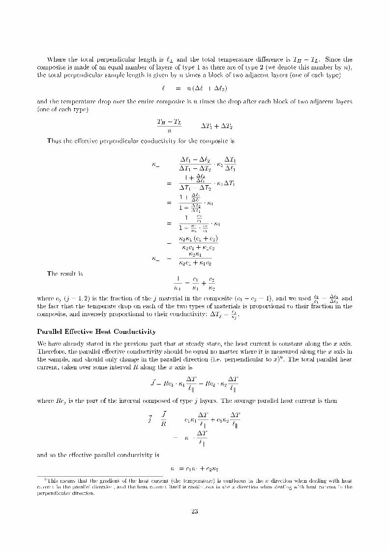
Where the total perpendicular length is `? and the total temperature di�erence is TH � TL. Since thecomposite is made of an equal number of layers of type 1 as there are of type 2 (we denote this number by n),the total perpendicular sample length is given by n times a block of two adjacent layers (one of each type)`? = n (�`1 +�`2)and the temperature drop over the entire composite is n times the drop after each block of two adjacent layers(one of each type) TH � TLn = �T1 +�T2Thus the e�ective perpendicular conductivity for the composite is�? = �`1 +�`2�T1 +�T2 � �1�T1�`1

= 1 + �`2�`1�T1 +�T2 � �1�T1= 1 + �`2�`11 + �T2�T1 � �1= 1 + c2c11 + �1�2 � c2c1 � �1= �2�1 (c1 + c2)�2c1 + �1c2�? = �2�1�2c1 + �1c2The result is 1�? = c1�1 + c2�2where cj (j = 1; 2) is the fraction of the j material in the composite (c1 + c2 = 1), and we used c2c1 = �`2�`1 andthe fact that the temperate drop on each of the two types of materials is proportional to their fraction in thecomposite, and inversely proportional to their conductivity: �Tj = cj�j .

Parallel E�ective Heat ConductivityWe have already stated in the previous part that at steady state, the heat current is constant along the x axis.Therefore, the parallel e�ective conductivity should be equal no matter where it is measured along the x axis inthe sample, and should only change in the parallel direction (i.e. perpendicular to x)9. The total parallel heatcurrent, taken over some interval R along the x axis is~J = Rc1 � �1�T`k +Rc2 � �2�T`kwhere Rcj is the part of the interval composed of type j layers. The average parallel heat current is then~j = ~JR = c1�1�T`k + c1�2�T`k= �k � �T`kand so the e�ective parallel conductivity is �k = c1�1 + c2�29This means that the gradient of the heat current (the temperature) is contiuous in the x direction when dealing with heatcurrent in the parallel direction, and the heat current itself is continuous in the x direction when dealing with heat current in theperpendicular direction.

23

Heat Transfer in a KettleClean KettleWater evaporates from a kettle at a rate � = 2 gmin�1. The bottom of the kettle is a copper plate of thickness` = 3mm and area A = 300 cm2. Copper is known to have heat conductivity �Cu = 5 J s�1 cm�1K�1. Thelatent heat of water is � = 2:25 J kg�1. What is the temperature on either side of the copper plate?At steady state, the heat current entering the kettle should be equal (due to conservation of energy) to theheat lost with evaporation: J = �� = 2 gmin�1 � 2250 J g�1 = 4500J min�1.On the other hand, the heat current entering the kettle should obey the heat equation, such thatq / �~rTJ = A��T�x�T = `JA��T = 3mm � 4500 J min�1300 cm2 � 5 J s�1 cm�1K�1 0:1mm�1 cm60 smin�1= 0:015KKettle with LimescaleThe same problem as before, only now a layer of thickness `scale = 1mm and heat conductivity �scale =0:0825 J s�1 cm�1K�1 separates the copper plate and the water. What is the temperature of the bottom ofthe copper plate and of the water touching the scale?In the case of the presence of limescale, we would have to use the result for the e�ective perpendicular heatconductivity through two layers of two di�erent type materials. In that case

�T = �x � JA�?= `JA

`Cu`�Cu + `scale`�scale!

Since `scale � `Cu but �scale � �Cu we could simply disregard the Copper, and calculate for the scale only�T ' `JA�scale= 4mm � 4500 J min�1300 cm2 � 0:0825 J s�1 cm�1K�1 0:1mm�1 cm60 smin�1= 1:21KThe full result, including the e�ect of the Copper as well as the limescale, would be not much di�erent.

3.2 Nonlinear Stationary StatesLinear problems can and should be solved by Fourier transforming the equation. We will consider time andspace independent sources only, Q (~r; t; T ) = Q (T ), but if these sources have a strongly non-linear dependenceon their argument, T , we will have to resort to other mehtods for a solution. We will further simplify ourproblem by discussing �rst the 1�D case � a thermally conducting wire (or thin cylinder).3.2.1 Current Carrying Superconducting WireA normal metalic wire with Ohmic resistance � is heated when a current with density j is run through it givinga heat source (heat release) with heat density QQ = � (T ) � j2

24

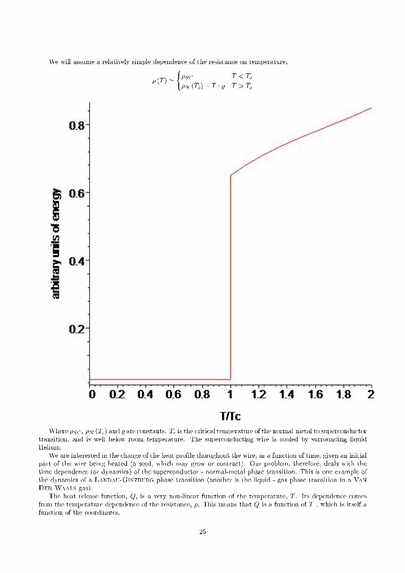
We will assume a relatively simple dependence of the resistance on temperature,� (T ) ' (�SC T < Tc�N (Tc) + T � % T > Tc

Where �SC ; �N (Tc) and % are constants. Tc is the critical temperature of the normal-metal to superconductortransition, and is well below room temperature. The superconducting wire is cooled by surrounding liquidHelium.We are interested in the change of the heat pro�le thorughout the wire, as a function of time, given an initialpart of the wire being heated (a seed, which may grow or contract). Our problem, therefore, deals with thetime dependence (or dynamics) of the superconductor - normal-metal phase transition. This is one example ofthe dynamics of a Landau-Ginzburg phase transition (another is the liquid - gas phase transition in a VanDer Waals gas).The heat release function, Q, is a very non-linear function of the temperature, T . Its dependence comesfrom the temperature dependence of the resistance, �. This means that Q is a function of T , which is itself afunction of the coordinates.25

The superconducting state satis�es �SC n �N , so that an extremely high current density can be reached.If heating in the superconducting state causes a temperature buildup beyond the critical temperature, Tc, thesudden switch to normal metal resistance will cause the wire to explode.We concern ourselves with a 3-D wire, but want to simplify the problem to a 1-D one. This can be done ifthe dynamics of the longitudinal heat transfer (along the wire) and the transverse one (in the cross section ofthe wire) have widely di�erent scales (of energy, time, etc.).C @T@t = �r2T +Q [T ]

= �0BBB@ @2@z2 + @2@y2 + @2@x2| {z }�r2?

1CCCAT +Q [T ] (3)Using the guidance of the Fourier heat equation, we assume the heat �ux in the surrounding liquid (and nearthe surface of the wire) to be linear in the di�erence between the temperature at the surface of the wire, Ts,and the temperature of the environment, T0. This is valid when the two temperatures are not very far apart.~qliquid? / Ts � T0We take the liquid heat conductivity as h, and write ~qliquid? ' �h (Ts � T0) � n, where n is the unit vectordirected from the center of the wire outward. From continuity of the heat �ux, ~qliquid? should be equal to boththe heat �ux in the liquid and in the wire, close to the surface.If the temperature within the wire cross section does not change much, we can write the transverse heat �uxin the cross section as ~qwire? = ��r?T� ���Tm � Tsb �where Tm is the temperature at the core of the wire (which is higher than Ts), and b is the radius of the wire.Equating the transverse heat �uxes at both sides of the surface of the wire10

��b (Tm � Ts) = �h (Ts � T0)Tm � TsTs � T0 = hb�If Ts ' Tm = �T we can assume the temperature throughout the corss section does not change much,in relation to the temperature di�erence between the wire and the liquid, �T � T0. The small parameternecessary for this approximation to be valid is the Biot number Bi � hb� � 1. If so, we can approximatethe temperature throughout a cross section at some point along the wire as constant for that cross section, i.e.�T (z; t) � 1A RR dxdyT (x; y; z; t).Averaging over each cross section in the heat transfer equation 3 yieldsC @ �T (z; t)@t = � @2@z2 �T (z; t) + �A ZZ dxdyr2?T (x; y; z; t) +Q � �T (z; t)�

The averaging of �Q [T ] ' Q � �T � is valid for a small Biot number�Q [T ] ' Q � �T �+ @Q@T �T � �T �+ : : : = Q � �T �+O �T � �T � = Q � �T �+O [Bi]10This is equivalent to expanding Tm as a �rst order expansion around Ts:

Tm ' Ts +r?T jR � b+ : : := Ts + h� (Ts � T0) � b

26

The only thing left is to de�ne the second term on the RHS as a function of �T . This is done using thedivergence theorem:� 1A

ZZ dxdyr2?T (x; y; z; t) � � 1AZZ dxdy~r? � h~r? � T (x; y; z; t)i

= � 1AI d}rnT (x; y; z; t)

= � 1A � C � 1h j~qj= 2�b� j~qj�b2h= 2� j~qjbh � �W � �T �In all we have C @ �T (z; t)@t = � @2@z2 �T (z; t) +Q � �T (z; t)��W � �T (z; t)�Where Q describes the heat release in the wire, and W describes the process of cooling to the external environ-ment. In the case of a wire of �nite thickness, the solution has got to be numeric.113.2.2 Chemical Reactions on the Surface of a CatalystOther applications of this method are exothermic chemical reactions of oxidation on a metal catalyst, such asPlatinum. Two such examples are:

2CO +O2 �!Pt 2CO24NH3 + 3O2 �!Pt 2N2 + 6H2OC2H4 + 3O2 �!Pt 2CO2 + 2H2OUnder some temperature, Tc, the catalysis is not e�ective. Above this temperature, the catalysis is e�ective,and the heat released in the reaction itself serves to keep the temperature of the catalyst hight.The dependence of the heat released in such reactions on the temperature at which the reaction is carriedout is similar to the function Q (T ) discussed for heat released in a metalic wire at temperatures below andabove the critical temperature of the normal-metal - superconductor phase transition. At low temperatures, Qis limited from kinetic considerations, while at high temperatures it is limited from di�usive considerations.12The catalyst facilitates the burning of exhaust waste after internal combustion. In some experiments, afocused laser beam is used to spark the burning on the surface of Platinum. The seed (spark) can thenpropagate over all the catalyst.

3.2.3 Metal - Dielectric Phase TransitionOne more example of such an application is the phase transition from a metal to dielectric in such compoundsas Vanadium Oxide, V nO. The heat released when an electrostatic �eld ~E is passed through the compound isdependent on the compound's speci�c heat coe�cient, �.Q (T ) = � (T ) � ��� ~E���2

The temperature dependence of � (T ) is similar to the resistance of the normal-metal - superconductor system,� (T ). For Vanadium Oxide, the hight temperature (metallic) conductance is ten orders of magnitude greaterthan the low temperature (dielectric) conductance.11In the fully linear case (i.e., Q is taken as a simple step function), this equation can be solved exactly:C @ �T (z; t)@t = � @2@z2 �T (z; t) +Q0 �� � �T � Tc�� CA � � � �T � T0�12See reaction-di�usion systems.

27

3.3 Linear Stability of Nonlinear Stationary States13Returning to the 1-D (longitudnal) heat transfer equation for the superconducting wire, we will look for somesimple solutions. For simpli�cation of notation, we will denote T = �T (z; t).To begin with, we will concern ourselves with spatially-uniform and time-independent solutions. This meansthat the terms @T@t = @2T@z2 = 0. A simple approach is to re-write the equation as Q [T ] =W [T ]. We plot both Qand W as functions of the temperature using the same axes. The solutions will simply be the intersects of thetwo graphs.

Clearly there are three such intersects:1. At T < Tc i.e. where the metal is a superconductor. We denote this temperature as TSC .2. At T � Tc i.e. near the superconductor - normal-metal transition. We denote this temperature at Ttrans.3. At T > Tc i.e. where the metal is a normal metal. We denote this temperature as TNM .13Appeared in 2007B.28

Furthermore, in the general case for a known material (% is known) diferent current densities, j, may be suchthat there are as few as one or as many as three intersects. Note the unique case of two such intersect points.

We now turn to study the stability of these solutions.14 In general we may check stability under smallperturbations or large perturbations. The latter cannot be done analytically, and computer simulations need tobe performed for speci�c large perturbations. However, the test for stability under small perturbations is morecrucial, since small perturbations always exists, and a system which is unstable under small perturbations willnot exist in the real world.Our equation (the heat transfer equation) is a linear equation, and we will assume linear perturbations ofthe form T (z; t) = Ti (z; t) + � (z; t)where Ti is a given equilibrium solution to be checked, and � is a small perturbation, i.e. �Ti � 1. Thelinearity of both the equation and the proposed solution gives a new heat transfer equation for �:C @�@t = �@2�@z2 +�@Q [T ]@T � @W [T ]@T � � �

since Q [T ]�W [T ] ' Q [Ti]�W [Ti] +�@Q [T ]@T � @W [T ]@T � � � +O "� �T �2#

and the non-�-dependent terms cancel with terms from the rest of the equation (assuming that Ti is indeedan equilibrium solution of the heat transfer equation).The heat transfer equation for � is a linear equation, and we guess a Fourier type solution � (z; t) ��0 exp (ikz + t) (i.e., Fourier transform in space and a Laplace transform in time of both sides of theequation). Clearly, the condition for stability is � 0, where the equality is meta-stable.14In all problems of a current carrying wire, we can tell experimentally if a state is unstable if the I � V curve has a negativeslope, i.e. negative resistance. The negative resistivity can be measured by adding a normal resistor in parallel such that the totalmeasured resistance is posititve, bu the normal resistor's resistance can be changed in order to measure the region of voltages forwhich the wire resistance in itself is negative.29

The transformed equation for � isC � = ��k2� +�@Q [T ]@T � @W [T ]@T � � � = ��k2C + 1C ��@Q [T ]@T � @W [T ]@T � � 0

The �rst term on the RHS of the last line contributes to stability. This term stems from heat dissipation inthe wire, away from the heated region, this heat counter�ow increases as k increases. To better understand thesecond term, we will treat the exterme case of k = 0, where the stability condition is simpli�ed to@Q [T ]@T � @W [T ]@T � 0@Q [T ]@T � @W [T ]@TTurning, again, to the graphic solution, we compare the slopes of Q and W at the three possible intersectionpoints. The conclusion is that the solutions at TSC and at TNM are stable, whereas the transition solution atTtrans: is unstable. The TSC solution corresponds to the whole wire being in the superconducting state with alow enough temperature throughout. The TNM solution corresponds to the whole wire being in a normal-metalstate. Can we derive solutions where the wire is partly at TSC and partly at TNM? How will these solutionschange in time?Universality with the time-independent Schrödinger EquationWe had C � = ��k2� +�@Q [T ]@T jTi � @W [T ]@T jTi� � �let's rename (x; t) � � (z; t)

C = � d2dx2+ � @@T fQ�Wg jTi� �E = � ~22m d2dx2+ V

The mapping to the Schrödinger equation is C 7�! �E� 7�! ~22m@@T fW �Qg jT=Ti 7�! VThe requirement of a solution to be stable is � 0, which in the case of the time-independent Schrödingerequation translates to it having a non-negative ground state energy, so that all the energy spectrum is non-negative E � 0 (C is always positive). Let's take a closer look at the limiting case of E = 0.For = 0 we had

0 = �T 00i (z) +Q [Ti (z)]�W [Ti (z)]taking the dirivative by z0 = � d2dz2T 0i (z) + @@Ti fQ [Ti (z)]�W [Ti (z)]g � T 0i (z)

which is an example of the time-independent Schrödinger equation with E = 0, where = T 0i . Let's examinethe solutions to this equation, and see whether they indeed are the ground state solutions, or if there could besolutions with E < 0, which entail system instability.1515The switching wave having an energy E = 0 can be explained by saying that the switching wave front is leading a macroscopic(say half) part of the sample. This is not a localized phenomenon, and therefore we expect it to have a low energy.30

The spatial derivative fo the switching wave soutions (which look like step functions) look like a deltafunction.16 This function has no nodes and therefore we conclude that it is indeed a ground state solution tothe relevant Schrödinger equation. That is, since we got this solution for E = 0, all the solutions obey E � 0,and this solution is stable.For a domain type solution (i.e. the region between two opposing fronts) the derivative looks like

This function has a node at z = 0, so clearly it cannot be a ground state solution. If this solution was gottenfor E = 0, than clearly there exists some other solution with E < 0, making the domain solution unstable.3.4 Propagation of Single Nonlinear �Switching� WavesIf we were to analytically solve the linear problem of the step function resistance (Q (T ) = Q0 � �(Tc � T )),we would solve for T > Tc and for T < Tc separately, and then match the two solutions at the point withT (z; t) = Tc. The location of this seam between the two regions (superconducting, and normal-metal) is time16The amplitude of the derivative function may seem large, but remember that all solutions can be scaled as we wish � it is onlythe functional form we are after.

31

dependent, therefore we have a moving front in the wire. This is a switching wave which travels through thewire at some velocity, v. We now try to �nd wave solutions of the form T (z; t) = T (z � vt) � T (�) to thenon-linear heat transfer equation CvdTd� = �d2Td�2 +Q [T ]�W [T ]We rewrite this equation as �T 00 = CvT 0 � fQ�WgThis equation has similar form to the well-known Newtonian equation for a driven and damped particle, or,the high friction limit of the Langevin equation 17

m�y = � _y + FThe mapping is T 7! y� 7! t� 7! m�Cv 7! �fQ�Wg 7! FNote that the friction coe�cient, = �Cv, can have either positive or negative sign, depending on the directionof motion, v.A di�erent mapping can �nd universality between our equation and the Schrödinger equation.3.3To gain physical intution as to the solution of this problem we concentrate on the last mapping.The potential energy surface on which the particle is moving is the integral over the force�rU (y) = F (y)

U (yf )� U (0) = �Z yf0 F (y) dy 7! Z Tf0 fQ [T ]�W [T ]g dTThe pseudo-�force�, F = �fQ�Wg looks like17Note that the friction coe�cient here is not the same as in the time dependence power e t we dealt with in the previoussection.

32

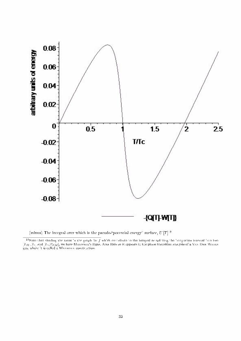
(minus) The integral over which is the pseudo-�potential energy� surface, U [T ]1818Note that shading the areas in the graph for f which contribute to the integral or splitting the integration interval into two[TSC ; Tc] and [Tc; TNM ], we haveMaxwell's Equal Area Rule as it appears in the phase transition analysis of a Van Der Waalsgas, where it is called a Maxwell construction.

33

A direct solution of the heat transfer equation can be helped along using integration of the entire equation:0 = Z 1�1 dzT 0 (z) f��T 00 (z) + CvT 0 (z)� [Q (T )�W (t)]g

= � (T 0 (z))2 j1�1 + Cv Z 1�1 dz (T 0 (z))2 � Z 1�1 dzT 0 (z) [Q (T )�W (t)]= Cv Z 1�1 dz (T 0 (z))2 � Z 1�1 dz dT (z)dz [Q (T )�W (t)]

v = R TNMTSC dT [Q (T )�W (t)]C R1�1 dz (T 0 (z))2Alternatively, we can observe that a freely moving particle on such a potential energy surface should obey34

conservation of �energy�, including the dissipated energy via the pseudo-�friction� term CvT 0U [TNM ]� U [TSC ] = Z TNMTSC CvT 0dT

U [TNM ] = Cv Z 1�1 T 0 dTdz dz1C U [TNM ]R1�1 [T 0]2 dz = vWhere we took U [TSC ] � 0 as a reference energy. The result is the velocity of a wave discribing the temperaturepro�le in the wire. The pro�le has tails at the two stable temperatures, TSC and TNM , and the disturbanceitself is a switching wave from one of the temperatures to the other.The sign of v de�nes the direction in which the switching wave propagates. It is also possible to get astanding wave with v = 0. This case maps to the case of = 0, for which the energy conservation criterion givesanother interesting insight: The transition time from one turning point (on the potential surface) to the other(i.e. TSC and TNM ) grows to in�nity as the energy of the particle travelling in the potential well between thesepoints nears the well depth. This is because the particle �feels� an increasingly anharmonic well as it investigatesthe walls of the well away from its minimum. At �rst these anharmonic e�ects only cause small deviations fromharmonic oscillations of the particle in the well, but as the particle energy grows and it investigates increasinglyhigher energies of the well, the approach towards each of the turning points becomes assymptotic.19 A particlestarting at TSC and rolling down the well towards TNM will never reach it, due to pseudo-energy considerations.That is, unless < 0 in which case the pseudo-friction force can actually push the particle �up-hill�, even pastTNM . All that's needed is the correct wave velocity, and a heating wave can actually switch the temperatureat a point on the wire form one stable value to the other.A combination of two such wavefronts leads to a temperature pro�le of a single domain of temperature TSC(TNM ) implanted in a wire at temperature TNM (TSC , respectively). When the initial heating of the wire createssuch a pro�le, we call it a �seed�. Depending on the velocities of the two wavefronts (call them vL and vR)the di�erent temperature seed, or domain, may shrink or expand. If vL = vR we have a di�erent temperaturedomain of �xed size moving through the sample. This wave is called a �soliton�.

19 This is a requirement on the pseudo-potential, needed so that the pseudo-force will be continuous even at the transition points.35

4 Di�usion in Momentum-Space4.1 Electron-Phonon Collisions in Metals at Low Temperatures20In a harmonic metalic solid with no defects, the mechanism for electron scattering is via interactions with thephonons. The electrons in the metal have characteristic energy of the Fermi energy, "F , and Fermi momentum,pF . Phonons in the solid have frequency !, and momentum ~q = ~~k, where ~k is the wavevector.The phonon spectrum is linear at small wavevector and energy: limj~kj!0 !~k = vs ���~k���, where the proportion-ality factor vs is the speed of sound in the solid. The low-frequency density of states is D (!) / !2, the Debyemodel assumes this can be extended until some cuto� frequency, !D, which is de�ned from the normalizationcondition on the sum of modes. Experimentally, this checks out to be fair.There is an interaction between the electrons and phonons, but the phonon energy is much smaller thanthe electron energy ~!D"F � 1, where !D is the maximal phonon frequency in the Debye model of a solid.Therefore the momentum transfer in an elecron-phonon interaction is much smaller than the fermi momentum:j�~pj = j~pf � ~pij = j~qj � pF . The small momentum transfer means that we can look at a single collision asa small change in the direction of the electron momentum. For a su�ciently small change, we can de�ne thesmall angle change as j'0j ' j~qjj~pj � j~pf � ~pijj~pijBecause the phonons are Bosons, the characteristic phonon average energy is proportional to the temper-ature, ~! � kBT . For temperatures much lower than the Debye temperature, i.e. kBT � ~!D � kB�D, onlythe lower frequency phonons are populated. This is the source for validity of the use of the linear dispersionreleation !~k = vs ���~k���.

vs j~qj = ~! � kBTj~qj � kBTvsThe electron Fermi energy is of the order "F � ~22ma2 , and the Fermimomentum is of the order pF � ~a � qD(where a is the distance between nearest neighbors, and qD is the Debye phonon momentum, which correspondsto the Debye phonon frequency !D). Note that the Fermi momentum, which is the characteristic momentumof the interacting electrons, is temperature independent.The temperature dependence of the small parameter '0 = qp :'0 (T ) = q (T )p (T ) � q (T )pF � kBTvspF � kBT~!D = T�D � 1

Therefor our constraint on the temperature (that it be much smaller than the Debye temperature) is consistentwith the requirement that the single collision direction change be small.We conclude that electron scattering by phonons consists of small collisions (where the momentum transferis small with relation to the initial and �nal electron momenta). This can be treated as a di�usion process inmomentum space (where each collision is a small step with step size of the momentum transfer).'2 (t)� = D' � tD' = '20��where '2 (t)� is the mean square of the direction change of a scattering electron after time t. Also, '20� is themean square of the direction change in a single collision, and � is the characteristic time between collisions.The macroscopic e�ect of the di�usion process will become appearent (and contribute to such macroscopicquantities as resistance and heat conductivity) only when ph'2 (t)i � 1 radian � 180�. We de�ne the timethis takes as t' � '2 (t')�D' � 1D' = �h'20i = ��kBT~!D �2 = �~!DkBT

�2 � � � �20Appeared in 2006B.

36

The temperature dependence of � (T ) is inversly proportional to the phonon density, which (since they areBosons) is proportional to T 3 (a sphere in momentum space, with radius kBT )� / 1nph: / 1T 3In all t' = �~!DkBT�2 � � / � 1T �2 � 1T 3 = 1T 5This result is attributed to Bloch.The Drude result for conductivity is �Drude = ne2�m , where n is the carrier density, e is their charge, m istheir mass, and � is the time between collisions. In our case, we will put � = t', so � = ne2m t' / T�5.

4.2 Relaxation of Heavy Particles in a Gas of Light ParticlesA small number of heavy gas particles with mass M (we denote their momenta as ~p) is surrounded in a largenumber of light gas particle of mass m (we denote their momenta as ~q).A collison (in one frame of reference) is depicted as follows: A heavy gas particle begins with momentum ~piand ends up with momentum ~pf . The participating light gas particle gains momentum ~q = ~pi � ~pf .Conservation of energy and momenta: p2i2M = p2f2M + q22m~pi = ~pf + ~qThe small parameter requirement for the validity of the treatment as a difusive process in momentum space:j~qjj~pij = 2mM+ 6 m ' 2mM � 14.3 Fokker-Planck Equation21Let's write an equation for the change in the fraction of particles with momentum ~p at time t, f (~p; t). Thischange is due to particles with momentum ~p + ~q losing momentum ~q (gain of particles with ~p), and particleswith momentum ~p losing momentum ~q (loss of particles with ~p). The rates of these processes are written asW (~p+ ~q; ~q) and W (~p; ~q), respectively. Assuming �rst order (linear) dynamics, i.e. @f@t / f , we get:@f (~p; t)@t = Z W (~p+ ~q; ~q) f (~p+ ~q; t) d~q � Z W (~p; ~q) f (~p; t) d~qWe will assume, as previously, j~pj � j~qj, and expand the integrands in series:

W (~p+ ~q; ~q) f (~p+ ~q; t) ' W (~p; ~q) f (~p; t) + 3X�=1 q� @@p� [W (~p; ~q) f (~p; t)]

+ 3X�;�=1 q�q� @2@p�@p� [W (~p; ~q) f (~p; t)]

From now on we will employ the Einstein summation convetion: a�b� =P3�=1 a�b�.Pluggin back into the kinetics equation we get@f (~p; t)@t = @@p��A�f (~p; t) + @@p� [B��f (~p; t)]�

A� � Z q�W (~p; ~q) d~qB�� � 12

Z q�q�W (~p; ~q) d~q21Appeared in 2006A, 2006B and 2007B.37

Where we identi�ed the constants A� and B�� as something akin to the �rst and second moments of therate W (~p; ~q), with respect to the second argument, ~q, only.We can also de�ne the respective current in momentum space,�j� � A�f (~p; t) + @@p� [B��f (~p; t)]

Such that @f@t = � @j�@p� ) @f@t + @j�@p� = 0is the momentum space distribution continuity equation.

Equilibrium boundary condition:At equilibrium we expect stationarity, @f@t = � @@p� j� = 0, and we denote the equilibrium momentum distributionf = f0. 0 = �j� = �A� + @B��@p�� f0 +B�� @f0@p�In a system with no external electromagnetic �elds, we have the equilibrium momenta distribution: The Boltz-mann distribution, f0 / exp�� p22MkBT � @f0@p� = � p�MkBT f0�A� + @B��@p�

� f0 �B�� p�MkBT f0 = 0This gives us a relationship between A� and B�� which holds for all f0 (~p).

A� = B�� p�MkBT � @B��@p�Putting this back into the kinetics equation we have the Fokker-Plank equation, to which we added anexternal force term22 @f@t = @@p��B�� � p�MkBT f (~p; t) + @f (~p; t)@p�

��� @f@~p ~FScattering of light particles o� heavy particles which is isotropic and independet of the heavyparticle's momentum W (~p; ~q) =W (j~qj) =W (q)Since B�� = 12

Z q�q�W (q) d~qwe see thatB�� / ��� .Or B�� = ���BB � 16

Z q2W (q) d~qbecause we have from isotropy that q2 = qxqx + qyqy + qzqz = 3 � qxqx22 @f@t = @f@~p @~p@t = @f@~p _~p = @f@~p ~F

38

Substituting into the Fokker-Plank equation,@f@t = B @@~p � ~pMkBT f (~p; t) + @f (~p; t)@~p �� @f@~p ~FAssuming a simple form of W (q) / �(q � q0) we can write an identity which connects the time betweencollisions, � , and the scattering rate, W :1 � � Z W (q) d~q1 = � � 4�3 q30

we already saw that B = q2010� , which means B can be thought of as some scattering length (a �one dimentionalcross section�).FIND REFERENCE FOR THIS IN LANGEVIN PART!!MobilityThe mobility is de�ned as h~vi = B � ~F , where the average velocity is de�ned (as are all the dynamic variables)by the (momentum) distribution function h~vi � R f (~p) � ~v � d~p.The deviation (response) of the distribution function from the equilibrium distribution (f0) due to a smallexternal force (perturbation) should be small, and linear in the disruption (perturbation).f = f0 + � f0 / ���~F ���plugging this into the Fokker-Plank equation, neglecting terms which are second order (in ���~F ���) and seeingthat the equilibrium terms cancel out,

B @@~p � ~pMkBT + @ @~p� = @f0@~p ~FThe solution is = ~p � ~FB f0

39

Kinetics

40

5 Boltzmann Equation5.1 Liouville's theoremWe discuss a system with N particles in phase space using 6N coordinates (positions qi and momenta pifor i = [1; 3N ] particles and spatial components). A point in phase space completely describes the entirecon�guration of the system. The system is de�ned using a Hamiltonian, H (qi; pi), and the equations ofmotion are the Hamilton equations:

_qi = @H@pi_pi = �@H@qiWe would like to write an expression for the probability for the system to be in the in�nitisimal neighborhoodof a certain point in our 6N dimentional phase space at a certain point in time, f (qi; pi; t). This equation is acontinuity equation dfdt +r (f~v) = 0where ~v is the generalized phase space velocity, and f~v is the phase space current. More explicitly,0 = @f@t + 3NX

i=1� @@qi (f _qi) + @@pi (f _pi)�

From the Hamilton equations we have0 = @@qi @H@pi � @@pi @H@qi= @ _qi@qi + @ _pi@piwhich we can arbitrarily choose to add to the phase space equation of motion

0 = @f@t + 3NXi=1� @@qi (f _qi) + @@pi (f _pi) + f �@ _qi@qi + @ _pi@pi

��to get

0 = @f@t + 3NXi=1� @f@qi _qi + @f@pi _pi

�what we actually got on the right hand side (RHS) of the equation is the total derivative, dfdt . This meansthat if we follow an in�nitisimal volume along its trajectory in phase space, we will see no change in the phasespace distribution f inside the volume. This is equivalent to comparing the phase space distribution to thedensity of an incompressible �uid in hydrodynamics.The spatial density of particles is simply the spatial part of the phase space distributionn (~r; t) = Z d~pf (~r; ~p; t)the energy current ~q (~r; t) = Z d~p~v" (~r; ~p; t) f (~r; ~p; t)

= Z d~p ~pm" (~r; ~p; t) f (~r; ~p; t)the electric current (particle charge times particle current)~j (~r; t) = eZ d~p~vf (~r; ~p; t)

= em Z d~p~pf (~r; ~p; t)In our discussion so far, we did not take into account any possible collisions. We will do so now.41

5.2 Boltzmann equationCollisions are non-local hops of the phase space distribution in time. For example, consider a binary collisionbetween a particle with initial momentum ~p and another particle with initial momentum ~p1 where their mo-menta after the collision are changed to ~p0 and ~p01, respectively. The rate of such a process may be written asW (~p; ~p1; ~p0; ~p01).Since this process should be time-reversible, we expect it to have the symmetry that if t is changed to �t andall momenta are given the opposite sign (e.g. ~p becomes �~p), nothing should be changed. Another symmetry weexpect this process to obey is invariance under spatial inversion: If all positions are inversed, and all momentaare inversed, nothing is changed (~r becomes �~r, and ~p becomes �~p).Time reversal symmetry means W of one process should be symmetric to its reverse process with ~pi �! �~pi(i.e., taking time and all momenta with opposite signs). Applying time-reversibility to W (~p; ~p1; ~p0; ~p01) givesW (~p; ~p1; ~p0; ~p01) =W (�~p0;�~p01;�~p;�~p1)Symmetry under spatial inversion means that W should be the same if all ~pi are exchanged with �~pi. Applyingspatial inversion symmetry to the result (from local isotropy) givesW (~p; ~p1; ~p0; ~p01) =W (~p0; ~p01; ~p; ~p1)The binary collision process gives the following phase space distribution time dependence: The density at acertain point in phase space is increased due to collisions which send particles to this point in phase space, anddecreased due to collisions which remove particles from this point.df (~p)dt = Z W (~p0; ~p01; ~p; ~p1) f (~p0) f (~p01) d~p1d~p0d~p01 � Z W (~p; ~p1; ~p0; ~p01) f (~p) f (~p1) d~p1d~p0d~p01= Z W (~p0; ~p01; ~p; ~p1) [f (~p0) f (~p01)� f (~p) f (~p1)] d~p1d~p0d~p01� St: ffgThe more explicit equation (known as the Boltzmann equation) is written as (in terms of a single particle'scoordinates) @f@t + @f@~r _~r + @f@~p _~p = @f@t + @f@~r ~v + @f@~p ~F = St: ffg

5.3 collision integralThe RHS of the Boltzmann equation is called the collision integral, or Stosszahl, and is physically problematicsince it suggests non-local e�ects have non-zero importance (i.e. the integration is done over all phase space,while we know that this cannot be right � we could put this information in the process rate, W ). In general,the collision integral may include many body collisions or interactions.At equilibrium, we expect dfdt = 0. From energy conservation for elastic collisions,(p0)22m + (p01)22m1 = p22m + p212m1

so we see that the equilibrium condition is met since the phase distribution at equilibrium f0 (~p) / exp�� p22mkBT �is such that f0 (~p0) f0 (~p01)� f0 (~p) f0 (~p1) = 0.Away from equilibrium, we have no idea how to solve the Boltzmann equation.5.4 �-approximationA simple model we can use instead of solving the collision integral is to assume a simple relaxation time, � , tothe equilibrium phase distribution dfdt = @f@t + @f@~r ~v + @f@~p ~F = �f � f0�

42

5.5 heat conductivity and viscosity of gasesAssuming a constant temperature gradient on the system of interest, we will consider the system at steady state(@f@t = 0), and disregard any other external forces (~F = 0). From the original, � -approximated Boltzmannequation, we are left with @f@~r ~v = �f � f0�we will, again, consider the linear response regime (f = f0 + , � f0). Substituting this into the previousequation, @f0@~r ~v + @ @~r ~v = � �we use the chain rule to write @f0@~r = @f0@T @T@~r = @f0@T � ~rTwe substitute back and get @f0@T � ~rT � ~v + @ @T � ~rT � ~v = � �however / ~rT and we will disregard the second term on the LHS since it is quadratic in the perturbation,O h(rT )2i.In order to discuss pure conduction, we need to disregard convection (radiation does not appear in thisproblem since we do not have a radiation �eld). To remove convection we need all the particle currents in thesystem to be zero, 0 = j = R d~p~vf . However, if we simply take j = ��rT = 0, we will also have rT = 0 andthen ~q = 0 which is a trivial and uninteresting answer, which we know is not the general result we are lookingfor. We can get a clue by looking at an ideal gas and noticing that the particle currents are zero if the pressureis spatially uniform. In the case of an ideal gas,P = nkBT0 = ~rP = ~rn � kBT + nkB � ~rT0 = ~rnn + ~rTT~rn / ~rTTherefore, we will expand our discussion from the system of equations~q = ��~rT~j = ��~rTto the system ~q = ��~rT + �~rn~j = ��~rT + �~rnThe phase space distribution function with respect to a system governed by the two thermodynamic variables,T and n leads to the following equation (via the chain rule)dfd~r = dfdT ~rT + dfdn ~rnwe will regard the phase distribution function in the linear response regime (f = f0 + ), where theequilibrium phase distribution function is given by the Boltzmann distriubution for an ideal gas,

f0 = n(2�mkBT )3=2 � exp�� p22mkBT

�Further, for a system under no external forces, and in steady statedfd~r~v = �f � f0��df0dT ~rT + df0dn ~rn� � ~v = � �

43

from the de�nition of f0 we also have df0dn = f0ndf0dT = f0T � p22mkBT � 32�

For an ideal gas we have (from the equation of state)~rnn = � ~rTTlet's try to guess a simple generalization of this for some non-ideal gas~rnn = � � ~rTTThe relevant Boltzmann equation is nowdf0d~r � ~v = f0T � � p22mkBT � 32 � � � �~rT� � ~v = � � (4)we will denote � = 32 + 23.

Particle CurrentThe particles phase space current density is ~j = Z ~vfd~p (5)where it is to be expected that at equilibrium the current is zero~j0 = Z ~vf0d~p = 0

therefore we only get a contribution from the term of the distribution function. Instead of plugging into5, we use 4 to write~j = �� Z ~v f0T � p22mkBT � ���~v~rT� d~p

or, in component notation (and using the Einstein summing convention for the index k)ji = �� Z vi f0T � p22mkBT � ���vk @T@xk

� d~pThe integral is anti-symmetric with respect to the indeces i and k, i.e. we only have a contribution from thethree cases of i = k (= x; y; z). Therefore, ji = � @T@xk �ikin the isotropic case, the non-directional term, �;24 is taken where v2i = 13v2 (from isotropy) and is thereforeindependent of i:

� = 13� Z 10 v2 � 1T n(2�mkBT )3=2 exp�� p22mkBT

� � � p22mkBT � �� � 4�p2dp= 43p� 1T n�(2mkBT )3=2

Z 10 v2 � exp�� p22mkBT� � � p22mkBT � �� � p2dp

= 43p� 1T n�(2mkBT )3=2Z 10 p2m2 � p2 � � p22mkBT � �� � exp�� p22mkBT

� dp23c.f. Heat capacity ratio (or adiabatic index).24c.f. Thermal expansion coe�cient

44

we perfom the change of variables u2 � p22mkBT� = 83p� n�kBm Z 10 u4 �u2 � �� e�u2du

= 83p� n�kBm8>>><>>>:Z 10 u6e�u2du| {z }�I(u6)

��Z 10 u4e�u2du| {z }�I(u4)9>>>=>>>;

The integrals are known (or can be worked out) and equalI �u4� = 3p�8I �u6� = 15p�16Therefore

� = n�kBm �52 � ��= n�kBm [1� ]

From which we see that for = 1 we get zero particle current, for all temperature pro�les.Energy Current

~q = Z ~v"fd~pWhere we will assume a monoatomic, free gas, " = p22m . Since the energy current is zero at equilibrium, we onlyget a contribution from (and not from f0)

~q = Z ~v" d~p= Z ~v"��� f0T � p22mkBT � ���~v~rT�� d~p= � �T Z ~v p22mf0 � p22mkBT � ���~v~rT� d~p

where in the second line, we have again used 4. Writing the result in component formqi = � �T Z vi p22mf0 � p22mkBT � ���vk @T@xk

� d~p= �� @T@xk �ikagain, from the anti-symmetry of the integrand with respect to the indeces i and k. The non-directional termK in the isotropic case is

� = 23p� n�mT (2mkBT )3=2Z 10 v2p4 � p22mkBT � �� exp�� p22mkBT

� d~p= 83p� n�k2BTm Z 10 u6 �u2 � �� e�u2du

with the same change of varialbes as for the particle current. We not also need the result of another integral,I �u8� = 15 � 732 p�

45

and we use the previous result (for the cancellation of particle current), = 1 to get� = 52 n�k2BTmSo we see that for = 1, � = 0 and � 6= 0, i.e. there is heat �ow but no net particle �ow.The mean time between collisions, � , can be de�ned from the thermal average velocity, hvi, and the meanfree path, `: � ' `hviwhereas the mean free path is related to the particle density, n, and the scattering cross section, �

` ' 1n�so that � ' 1n� hvithis means that � = 52 k2BTm� hvi / pTthe heat conductivity is proportional to the square root of the temperature, and is independent of the particledensity.It should be emphasized that the entire derivation is only valid where the temperature gradient is small onthe length scale of the mean free path �TL � �Twhere L is the length scale over which the gradient is computed.Qualitative Explanation of the DynamicsThe particle �ux through a point, x0, in the positive x direction isq+x (x0) = n6 hviC [T (x0 � `)]where, in the isotropic case, the chance that a particle moving through x0 is moving in the positive x directionis 16 . Further, we allowed the heat capacity to have a temperature dependence, and its e�ect is taken over aparticle comming into x0 from ` away, and travelling with thermal speed hvi.q�x (x0) = �n6 hviC [T (x0 + `)]The net energy current in the x direction is

qx (x0) = n hvi6 fC [T (x0 � `)]� C [T (x0 + `)]gExpanding the temperature pro�le in Taylor series,T (x0 � `) = T (x0)� `@T@x jx0 +O ��@2T@x2 ��The �rst term in the expansion is cancelled in the net current

qx (x0) = n hvi6��2 � dCdT `dTdx�

= � n hvi `3 dCdT| {z }��dTdx

� ' hvi3� dCdT / pTand we have the same dependence of � on temperature and independence of particle density that we got before.46

Microscopic Derivation of ViscosityViscosity can be seen, for example, in a �ow through a cyllindrical pipe, where the velocity pro�le in a crosssection of the pipe is such that the velocity at the boundary is zero, and the velocity at the center of the pipeis heighest. Nearby particles �owing at di�erent distances from the center of the pipe (i.e. particles �owingin neighboring radial layers) a�ect each other via shear forces, which are proportional to @ux@z x, where x is thedirection of the �ow (along the pipe), and z is the radial direction.A microscopic explanation is that due to di�usion in the z direction, there is a momentum transfer in the xdirection � this is because the momentum in the x direction px, is a function of z. Since _px is nonzero, we saythat there are forces in the system which cause this change, and call these shear forces.The momentum �ux (which is the shear force) in the x direction, in a layer at distance z from the center ofthe pipe, is a�ected by the di�usive current between neighboring layers (at z � `) in the z direction, and themomentum in the x direction in each of these layers.pzx = 16n hvimux (z � `)| {z }px(z�`) �16n hvimux (z + `)| {z }px(z+`)= � 13n hvim`| {z }��

@ux@z� = m hvi3� = hpi3� / pT

And the viscosity coe�cient, �, is proportional to the square root of the temperature, and independent of theparticle density.Viscosity from the Distribution FunctionThe momentum �ux pik = Z mvivkfd~pThe Boltzmann eaquation in steady state, no external forces, and linear response regime@f@z vz = � �The equilibrium phase space distribution is the Boltzmann distribuion only in a system at rest. We need toswitch to a shifted function with respect to the moving frame of the bulk �ow, which is dependent on the zcoordinate f0 = f0 (vx � ux (z) ; vy; vz)we de�ne the variables Ux = vx � ux (z)Uy = vyUz = vzsuch that equilibrium in the moving frame of the liquid means hUxi = hUyi = hUzi.The chain rule gives (neglecting second order terms)@f@z = � @f0@Ux @Ux@zAnd the Boltzmann equation is @f0@Ux @Ux@z Uz = �

47

The momentum �ux ispzx = Z UzmUxfd~p

= Z UzmUx� @f0@Ux @Ux@z Uzd~p= �@Ux@z �

0BBB@�m� Z U2zUx @f0@Ux d~p| {z }��1CCCA

The viscosity coe�cient is� = �m� Z U2zUx @f0@Ux d~p= m� Z U2z f0d~p

= 13�m Z U2f0d~p= 23� h"Kinin

where in the second line we performed integration by parts, and in the third line we took the system to beisotropic. In the last line we get n from the normalization factor of f0 = n � exp ��p2=2mkBT �. If the systemis in thermal equilibrium, h"Kin:i = 12kBT� = 13�kBTn' 13 `hvikBTn' 13 1hvi 1n�kBTn� / kBThvi� / pTOnce more, we see that the viscosity coe�cient is proportional to the square root of the temperature andindependent of the particle density.

48

6 Kinetics of a Degenerate Electron GasThe conduction electrons in a metal can be considered as a degenerate electron gas (DEG). The DEG ischracterized by an equilibrium phase space distribution function which is the Fermi-Dirac distribution, andfor reasonable temperatures is very close to a step function of the energyf0 ("; �; T ) � 11 + exp� "��kBT �f0 ' �("F � ")

�@f0@" ' � ("� "F )The Fermi energy (above which the population is zero) is close to the chemical potential for the reasonabletemperatures mentioned above, kBT � "F ' �. We will interest ourselves in the response of the DEG systemto perturbations characterized by even smaller energy �"� kBT .The Sommerfeld expansion will be relevant to all of the calculations we will perform for any variable, A (")

�Z 10 d"A (") df0d" = A (�) + �26 (kBT )2 d2A (")d"2 +O "�kBT� �4#for instance, � = "F � �26 k2BT 2 �0 (")� (") j"="F (6)where " = p22m and � is the density of states (DOS), such that in 3-D � (") / p".6.1 Electrical and thermal conductivities25The Boltzmann equation in the linear response regime (f = f0 + ) or � -approximationdfdt = @f@t + @f@~r ~v + @f@~p ~F = �f � f0� = � �The external electric �eld is weak if eE`� "FAdditionally, we will require e�cient heat removal from the metal.DEG Electrical ConductivityThe Boltzmann equation for a spatially uniform and time constant external electric �eld becomes

� � = @f@~p ~F= @f@~p e ~E= @f0@~p e ~E +O �� ~E�2�= @f0@" @"~p e ~E= @f0@" e~v � ~E25Appeared in 2007A.

49

The electric current density is~j = Z e~vfd~p

= Z e~v d~p= eZ ~v ��� @f0@" e~v � ~E� d~pIn component notation

ji = e2� Z d~p��@f0@" � vivkEkji = �ikEk�ik � e2� Z d~p��@f0@" � vivkIn the isotropic case the conductivity tensor is�ik = ��ik� � e2� Z d~p��@f0@" � v23= e2�3 Z d"� (")��@f0@" � 2m"

Taking only the �rst term in the Sommerfeld expansion� = 2e2�3m Z d"� (") � ("� "F ) "

= 2e2�3m � ("F ) "F' e2�m n"F "F= ne2�mwhich is the classical Drude conductivity.

DEG Heat Conductivity26In steady state and with no external forces� � = @f@~r � ~v= �@f0@T ~rT + @ @T ~rT� � ~v = �� @f0@T �~v � ~rT�where in the middle line we used the chain rule and threw away second order terms in ~q / ~rT (it is assumedthat ~q is zero in equilibrium and that is linear in the perturbation, ~q).26Appeared in 2006A.

50

Now, @f0@T = @@T 11 + exp� "��kBT �= @f0@� � @�@T j�= "��kBT= kBT @f0@" � @@T "� � (T )kBT= kBT @f0@" �

"� "� �(kBT )2 � 1kBT @�@T#

= �@f0@" � �"� �kBT + @�@T �The �rst term in the square parentheses is of order unity, the second is of the order of kBT"F � 1 (this can beveri�ed from the Sommerfeld expansion of �). Therefore, we will neglect the second term with respect to the�rst one and get ' � "� �kBT @f0@" �~v � ~rT�The heat current is calculated by~q = Z ~v ("� �) fd~p

' Z ~v ("� �) � ("� �)kBT @f0@" �~v � ~rT� d~pqi = Z � ("� �)2kBT @f0@" vivk| {z }��ik@T@xk d~p

qi � ���ik @T@xkwhere in the last line we assumed isotropy. We continue in calculating �.The �rst order Sommerfeld expansion for the heat conductivity (�) contributes nothing, as it is just theequilibrium term (� (" = �)). The next term is proportional to @2�@"2 j"=�, which means the ("� �)2 is expectedto drop out in the �nal result.� = Z � ("� �)2kBT @f0@" v23 � (") d"

= � 2kBT �26 (kBT )2 v23 � (�)= �29 �v2� (�) k2BT

6.2 Wiedemann-Franz law27In the previous section we got

� = e2�3 v2� (�)� = �2�9 v2� (�) k2BTThe Wiedemann-Franz law states that �� = �23 k2Be2| {z }�L T / T

27Appeared in 2007A.51

where the proportionality constant L is independent of the material. At low temperatures, the number of exitedphonons is / T 3 while the heat conductivity contribution from the electrons alone is / T , and so electronicheat conductivity is measureable directly at low temperatures. Since the heat conductivity of a only the DEGin a sample is extremely hard to measure directly at higher temperatures, we can use the Wiedemann-Franzlaw and much easier electrical conductivity measurements to get the result indirectly.6.3 Skin-e�ectFor time and space dependent �elds we will look at an electromagnetic wave impinging on a metal. Since theconduction electrons are very nearly free, in equilibrium they will reorient themselves to cancel out any �eld inthe metal, and do so on a time scale faster than any other time scale in the problem, therefore for all purposes,~E = ~B = 0 in the bulk metal. Still, this e�ect is not ideal in a real metal (in which the electron have a �nitemean free path, ` < 1), and therefore there is room to compare the wavelength of the electromagnetic wave,�, with its penetration depth or skin depth, �.If the particles contributing to the conductance, �, have a mean free path, `, much smaller than the skindepth, �, then those particles indeed feel a uniform electric �eld, ~E, and are unaware that at a distance muchgreater than � into the metal, ~E = 0.Another way of looking at this is,1. If the metal is far from ideal (� � `) we can assume ~j (~r) = � ~E (~r), i.e. since there are many electroncollisions in the skin layer, the dependence of ~j on ~E is local.2. If the metal is nearly ideal (� � `) we cannot assume such a local dependence, and we have to write~j (~r) = R � (~r; ~r0) ~E (~r0) d~r0. We expect an electron moving within the skin layer to be a�ected by theimpinging electromagnetic �eld, and to be accelerated by it, while an electron much deeper in the metalto be una�ected by the �eld.The electric �eld outside the metal is made up of the incoming wave (E1) and a re�ected wave (E2), withwavevector k and frequency !, and the electric �eld inside the metal (in the skin layer) has the same frequencybut a di�ernet wavevector q28. At a distnace into the metal which is greater than the skin depth, the electric�eld is assumed zero. This means that the electric �eld in the metal would look something like an oscillatory�eld, con�ned by an exponentially diminishing envelope28The exterior vacuum has the dispersion relation ! = ck. In the metal, a wave with wavevector q has the frequency !.

52

We take the direction of the waves (y) to be perpendicular to the metal surface, and writeEout = E1 exp (iky � i!t) + E2 exp (�iky � i!t)Ein = Em exp (iqy � i!t)This is a purely electromagnetic problem, so we employMaxwell's equations. If we useOhm's law, ~j = � ~E,and from Maxwell's equations we get

~r� ~E = �1c @ ~H@t~r� ~H = 4�c ~j + "c @ ~E@t' 4�c � ~E + "c i! ~E= 1c (4�� + i"!) ~E53

since in a metal � � 1020 in cgs units, but ! � 1010 in cgs (or MKS) units,~r� ~H ' 4��c ~E

~r� ~r� ~E = �4��c2 @ ~E@tr2 ~E = �4��c2 @ ~E@twhere in the last line we used the fact that in the metal @�@t = 0) ~r �~j = 0) ~r � ~E = 0.plugging Ein into the expression for ~E we get

�q2Ein = �4��c2 i!Einq = pir4��!c2

= 1 + ip2r4��!c2and since Ein / exp (iqy) we write

Ein = exp � [1� i] p2��!c � y � i!t!

= exp0BBB@i � p2��!c| {z }���1in

�y1CCCA exp

0BB@� p2��!c| {z }���1 �y1CCA exp (�i!t)

/ e�y=�so the skin depth is de�ned by� = cp2��!/ 1p!

where in the last line we used the fact that the Drude conductivity �� = ne2�m � is frequency independent. Notethat since <e (q) = =m (q), we have � = �inn �out.29We de�ne the impedance as the ratio between the electric �eld strenght at the surface and the total inducedcurrent running parallel to the surface.Z � Em (y = 0)R ~j (x; y; z) dy

= Em (y = 0)R10 ~j (y) dy= Em (y = 0)R10 c4� @ ~H@y dy= Em (y = 0)c4� h0� ~H (y = 0)i= �4�c Em (y = 0)H (y = 0)29For instance, for an impinging radio wave with �out = 1m = 102 cm, and therefore ! � 2� 109Hz, and for a metal in which` � 10�3 cm meaning � � 1022 cgs ' 108m�1 �1, we get � � 10�5 cm � 10�7 � �out.

54

Since all of the �elds (E1, E2, Em) have an oscillatory time dependence,@E@y = 1c @H@t= 1c (�i!)Hic! @E@y = HZ = �4�c Em (y = 0) !ic �@E@y jy=0��1

= 4�i!c2 Em (y = 0)@@yEm (y = 0)= 4�i!c2 Em (y = 0)iqEm (y = 0)= 4�!c2q� 4�!c2 � � � p!

At the surface of the metal, both ~E and @@y ~E are continuous. Since @ ~H@t / @ ~E@y , ~H is also continuous acrossthe surface. Ein (y = 0) = Eout (y = 0)@Ein@y jy=0 = @Eout@y jy=0We would like to know the ratio of the amplitudes of the electromagnetic �eld in the metal and the re�ected�eld. The di�erent �eld amplitudes are measureable experimentally. This allows very precise measurments (upto 10�12m!). E1 (y = 0) + E2 (y = 0) = Em (y = 0)ik [E1 (y = 0) + E2 (y = 0)] = @@yEmjy=0 = iqEm (y = 0)

therefore,2E2 (y = 0) = Em (y = 0) + @@yEmjy=0ikEm (y = 0)E2 (y = 0) = 21 + 4�c 1Z ' c2�Z � �� � p! � 1

The discussion so far discussed what is called the normal skin e�ect. But recall that we invoked Ohm's law,which applies only in the case of a very non-ideal metal (� � `), i.e. all through the skin layer the local Ohm'slaw applies. However, what happens for a nearly ideal metal (� � `) ?Because of the large mean free path, only a small fraction of the carriers travel in a direction which hasa signi�cant component parallel to the surface (such that they spend enough time near the surface, and theincoming electric �eld can signi�cantly bestow energy to the carriers). This fraction of e�ective carriers isde�ned according to the e�ective skin depth, �eff:, which we will venture to �nd.neff:n � �eff:` � 1Only this fraction will contribute to the induced current parallel to the surface. The rest escape deeper intothe bulk and are lost to us thereafter (since ~E = 0 in the bulk, these carriers will not come back to the skin

55

layer). Although the fraction of participating particles (neff: � �eff:` n) is small, their contribution to the overallconductance is much greater than the contribution of the other particles,nineff: = n� neff:= n �1� �eff:` �

nineff: �1 + �eff:` � ' nTHE FOLLOWING LINE DOES NOT CHECK OUT!

�ineff: � nineff:e2m `vF + �eff:` � ne2m �eff:vF = neff:e2m vF � �eff:The conductance of the e�ective carriers is

�eff: ' neff:e2�m' neff:e2m `hvi� neff:e2m vF� ne2m �eff:` vF= ne2m �eff:vFTherefore, we have the e�ective conductance in terms of the e�ective skin depth. We will now use the moregeneral relation between the two, which we found in our analysis of the normal skin e�ect:

�eff: = cp2��eff:!= cp2�!r mvFne2�eff:

�3=2eff: = r mc2vF2�ne2!�eff: = � mc2vF2�ne2!�1=3 / 1!1=3 � 1p! / �

As it turns out, for an impinging electromagnetic wave of frequency !, while the skin depth was � / !�1=2for a very non-ideal metal, for a nearly ideal metal it is � / !�1=3 . Moreover, in the case of a nearly idealmetal, the skin depth is independent of the mean free path, `.The Boltzmann equaition was initially described using one unavoidable parameter � the mean time betweencollisions, � . Note that the � (or `) dependence in �eff: cancels out. This means that the �anomalous skin e�ect�is valid also for resistance-less physical systems, such as superconductors, super�uids, etc. where there is nosuch �time between collisions�.6.4 Electrical Conductivity in a Magnetic FieldThe classical motion of an electron in a magnetic �eld (we will take it in the z direction, as a standard) and inthe absence of an electric �eld is a rotation in the x� y plane with radius of gyration

R = mv?eBwhere v? is the tangent velocity. We denote the angular frequency of the rotation (the cyclotron angularfrequency) with � eBmc . If the time between collisions is � , then the criterion for a �strong� �eld is � � 1.56

This can be translated to R � `, where ` is the mean free path. The picture is of electrons rotating in circlesin the x � y plane of radii R (v?), and a translation of the center of the circle once in a while (the result of acollision).In the absence of the magnetic �eld, the conductivity is given by the Drude conductivity�0 = ne2�mSince the magnetic �eld only a�ects the motion of the electrons in the x � y plane, the conductivity tensor inthe case of both magnetic and electric �elds will have an unchanged �zz = �0 component.In the presence of an electric �eld ~E = Ex, we can always perform a Lorenz tranformation to a framewhere there is no electric �eld. ~E0 = 0 = ~E + ec~u� ~B

0 = E + ecuyBuy = � ce EBIn this system (in the laboratory frame) there is an e�ective drift currentjy = neuy= �ncB|{z}��yx EThe induced current in the negative y direction in response to an electric �eld in the x direction is called theHall e�ect.We will now treat the problem using the Boltzmann equation approach.In the case of strong �elds, the general picture is of an electron rotating around its center, in the x�y plane.It manages to complete many periods of rotation between collisions, which simply translate the center of itsrotations. In the case of weak �elds, the electron hardly completes one rotation between two collisions, so theoverall trajectory looks very similar to the case of H = 0. As opposed to the weak �eld, or no �eld case, theelectron trajectory in a strong �eld is very much localized around one center, so the mean free path ` should bereplaced by the trajectory length scale, R. In this case the Drude conductivity becomes� = ne2�m ' ne2m `hvi ' ne2m Rhvi ' ne2m 1Since the most an electron moves under such a strong �eld is from one side of the circle to the opposite side, adistance of 2R, this should de�ne the mean free path and di�usion constant D = `2=� ' R2.For spatially uniform and time independent �elds in steady state@f@~p ~F = �f � f0�~F = e ~E + ec~v � ~B@f@~p �e ~E + ec~v � ~B� = �f � f0�This equation is an equation for (px; py; pz). Clearly, the cartesian basis is not the optimal one for thisproblem (recall the electrons rotate in the x � y plane). For an electric �eld in the positive x direction andmagnetic �eld in the positive z direction, ~E = Ex~B = Bz) _pz = 0pz = const:

57

therefore, pz would be a convinient coordinate to keep. Another usefull coordinate is the phase of the particlein the rotation cycle, '. d'dt = The third coordinate will be the energy, ", and _" = e~v � ~E, since it too is conserved for the unperturbed case( ~E = 0). d~p = eBc dtdpzd"

dfdt = @f@t _t+ @f@~r _~r + @f@~p _~p = �f � f0�dfdt = @f@'+ @f@pz 6 _pz + @f@" �e~v � ~E� = �f � f0�The pz drops since _pz = 0, and from the dfd" term we neglect the contribution which is second order (in E) andare left with df0d" . @f@t + @f0@" �e~v � ~E� = �f � f0�@f@t + @f0@" �e~v � ~E� = � �@ @t + � = �@f0@" �e~v � ~E�where in the last line we used f = f0 + . We de�ne a new variable, �, such that30

= �@f0@" �we now have @�@t + �� = e~v � ~E = _"to which the solution is

�(t) = Z t�1 _" (t0) exp�� t� t0� � dt0= Z 10 _" (t� t0) e�t0=�dt0

The current in component notation is = �eEk @f0@" Z 10 vk (t� t0) e�t0=�dt030This means that f = f0 � @f0@" �+O �� ~E�2�and therefore � is the �rst order expansion of f ("), or in other words� � ". We can then write (to �rst order)

f = f0 ("��) = f0 � ["��]� �kBT�

so � is simply an energy shift in the distribution function. It can also be thought of as a shift in the chemical potential (or electricpotential) �+� = �+ eV

58

ji � jeq:i = ji = Z evi d~p(2�~)3= �e2 Z d~p4�3~3 vi @f0@" Z 10 vk (t� t0) e�t0=�dt0Ek= �ikEk�ik � � e24�3~3 Z d~p@f0@" vi Z 10 vk (t� t0) e�t0=�dt0= � e3B4�3c~3 Z 10 d"@f0@" Z 1�1 dpzvi (t) Z 10 vk (t� t0) e�t0=�dt0= � e3B4�3c~3 Z 10 d"@f0@" Z pz�pF dpz

Z T= 2�0 dtvi (t) Z 10 vk (t� t0) e�t0=�dt0Where the Jackobian was calculated as

d~p = md" � dpz � �d'z}|{dt= eBc d"dpzdtFor a spherical Fermi surface, vx = v? cos (t)vy = v? sin (t)v? ("; pz) = 1mp2m"� p2zthe conductance tensor components are, for a strong �eld

�xx = �yy = �0 11 + (�)2 ' ne2�m 1(�)2 / 1B2�xy = ��yx = �0 �1 + (�)2 ' ne2�m 1� = ne2m = necB / 1B�zx = �zy = 0

The regular conductance is independent on the sign of ~B, because the correction is quadratic in B, whilethe Hall conductance is linear in B, and therefore antisymmetric in ~B.The strong �eld Hall conductance is independent on the time between collisions, �; or on the carrier mass,m, but can be used to measure carrier density and sign (antisymmetric in ~B).The weak �eld case (� � 1) indeed gives small corrections to the zero-�eld case�xx = �yy = �0 11 + (�)2 ' �0 h1� (�)2i�xy = ��yx = �0 �1 + (�)2 ' �0� � �0�zx = �zy = 0The regular conduction is slightly �damped� and the Hall conductance, linear in the �eld strength, is stillmuch smaller than the regular conductance.

�xx � �0 = �yy � �0 / 1B2�xy / 1B59

Discussion of the Hall e�ectSuppose we have an electrical circuit set up in which a sample of suitable material is connected to an electricsource, and we can control the electric �eld on the sample and measure the electric current in it, both taken inthe direction from one connection to the circuit to the other (call it the x direction).The whole system is immersed in a constant magnetic �eld, H, in the z direction. Since we deal with asteady state, the Hall current, jy, is zero. On the other handjx = �xxEx + �xyEyjy = �yxEx + �yyEy = 0So we have the induced Hall �eld Ey = ��yx�yyEx / HWhere the Hall �eld is linear in the magnetic �led, according to linear response.Now,

jx = �xxEx � �xy �yx�yyEx= �xx�yy � �xy�yx�yy Ex

Taking our previous results�xx = �yy = �0 11 + (�)2�xy = ��yx = �0 �1 + (�)2substituting these into our result for jx we have

jx = �xx�yy � �xy�yx�yy Ex=

h �01+(�)2 i2 + h �0�1+(�)2 i2�01+(�)2 Exjx = �0ExSurprisingly, there is no dependence on the magnetic �eld, H!A qualitative explanation Under strong �elds, � � 1 so that

�xx = �yy ' �0 1(�)2 / 1H2�xx = ��yy ' �0 �(�)2 = �0 1� / 1H

�ik '0@ �0 ��0H 0�0H �0H2 00 0

1Aso, for strong magnetic �elds, the dependence of the Hall conductivity is inverse in the �eld. The more generaldependence of � on H is

60

That is, a very weak dependence on the magnetic �eld strength, H.The electron's trajectory is de�ned by cuts in phase space which are perpendicular to ~B k z k ~pz. Fora spherical Fermi surface this meant that the electron moves in a circle around the z axis at some constantvalue of pz. If the Fermi surface is not a sphere, but rather something like a 4-way (cross shaped) pipe-pipeintersection

61

then if the cut is made close enough to z = 0, the trajectory will look like two disconnected lines, onefollowing the contour begining at some positive value of x and y and the other at the opposite value of x andy. The trajectory on either one of the lines will never reach the other line, since they are disconnected withinthis lattice cell. However, we know that the electron has to move in some closed orbital.This orbital will not be closed over one lattice cell, but will continue on to the next cell, and so on. Thismeans these electrons go on conducting for great distances with no damping of their regular conductance. Onesuch example is Copper.6.5 Onsager relations31We have seen that in response to various external �elds or forces ( ~E; ~rT; ~rn; : : :) we get various currents in thesystem (~j; ~q; : : :). We now generalize these relations to generalized forces Xi which induce generalized �uxes Ji.We assume that these generalized forces create a linear response, and that we can express this response as alinear combination of the induced generalized �uxes. That is,Ji = � ikXk(where the Einstein summation convention is implied).We also assume that the change in the system entropy (or irreversible heat) is given by_S = �JiXi = ikXiXkunder the assumption that the change in entropy is symmetric in the sign of the external �eld32,

ik � ~X� = ki �� ~X�we can deduce that the matrix is symmetric ik = ki31Appeared in 2007A.32An example we saw before was the Hall conductance: �xy � ~B� = ��yx � ~B� = �yx �� ~B�

62

The conclusion is that there are fewer degrees of freedom to a system than appear to be (assuming theentropy of the entire system remains constant).To illustrate this formalism we will give the simple example of electrical conductivity,ji = �ikEkde�ningXi = �EiTJi = ji ik = T�ikwe can write Ji = ji = �ikEk= � (T�ik)��EkT �= � ikXk_S = ikXiXk= T�ik ��EiT ���EkT �

= 1T Z jiEid~rFrom the symmetry of the matrix we get the same symmetry for the conduction tensor �ik = �ki.6.6 Thermo-Electrical PhenomenaGiven a temperature gradient, ~rT , and an electric �eld, ~E, the electric and heat currents are, respectively~j = � ~E + �~rT~q = � ~E � �~rTwe de�ne the Onsager variables ~J (1) = ~j~J (2) = ~q~X(1) = � ~ET~X(2) = � ~rTT 2substitiuting these back into the equations for ~j and ~q,J (1)i = ji = �Ei + �riT

= (�T�)��EiT �+ ��T 2��riTT 2 � (1;1)ik = �T�ik (1;2)ik = T 2�ikand J (2)i = qi = �Ei � �riT= (�T�)��EiT �+ ���T 2��riTT 2 � (2;1)ik = �T�ik (2;2)ik = �T 2�ik

63

In all, = � �T� T 2��T� �T 2� �From the symmetry of implied by the Onsager relations (2;1) = (1;2)� = �T�The entropy of this system increases due to Joule heating and decreases due to heat dissipation_S = Z ~j � ~ET d~r � Z ~r � ~qT d~r

= Z ~j � ~ET d~r + Z ~q � ~r� 1T � d~r= Z ~j � ~ET d~r � Z ~q � ~rTT 2

! d~r= �Z "~j � � ~ET

!+ ~q � ~rTT 2!# d~r

where in the second line we integrated by parts, and �nally we arrived at the requiered form.Since in this case the electric current is more easily measurable than the electric �eld, we rewrite ourequations as~E = �~j �Qz}|{��� ~rT~q = ��|{z}�� ~j � �~rT

we already discussed the fact that � = �T�; and therefore � = TQ. In all we have~E = �~j +Q~rT~q = �~j � �~rTAs an example, suppose we have a material held at a constant, non-zero, temperature gradient (~rT ), andan electric �eld (given, for example, by an electrostatic potential, ') imposed on the material such that theoverall electric current through the material is zero, ~j = 0.�~r' = ~E = �~j +Q~rT= Q~rTAssuming the direction of the temperature gradient is the direction of the electric �eld (call it x). Using thechain rule,

�d'dx = QdTdxd'dT = �QThe quantity Q is called the thermoelectric power, or thermopower33. For a metal it can be calculated

Q ' �23e k2BT� (n) � �10�8 VK� � T33The use of the term �power� is misleading.64

Peltier E�ectA contact is set up between two di�erent materials, a and b, with di�ering � values, �a 6= �b. An electricalcurrent (~j) is applied which �ows from one material to the other. Since the temperature gradient across thecontact, �~rT = ~q should be equal on both sides of the contact0 = ~qa � ~qb = (�a ��b)~j �WThe only way for the temperature gradient to remain constant across the contact is for an excess heat to begiven o� at the junction itself, W . This is one method of welding.

Thomson E�ect34We generalize our initial thermoelectric example to the case of a non-zero temperature gradient and a spatiallyconstant electric current, ~r �~j = 0. The heat release from the sample was given asw = _s = ~j � ~E � ~r � ~q= �j2 +Q~j � ~rT � ~r � ��~j�+ ~r � ��~rT�= �j2 +Q~j � ~rT �~j � �~r��+ �r2T

the term proportional to ~r �~j = 0 drops due to Maxwell's equations. And sinceQ~j � ~rT �~j � �~r�� = Q~j � ~rT �~j � �d�dT ~rT�

= �Q� ddT (TQ)�~j � ~rT= �Q�Q� T dQdT �~j � ~rT= �T dQdT ~j � ~rTwe get W = �j2 � T dQdT ~j � ~rT + �r2T

where the �rst term is the Joule heating, the second term is anti-symmetric in the direction of ~j, and the lastterm is symmetric in the direction of ~j.

34William Thomson was the Lord Kelvin, and he predicted and observed this e�ect in 1851.65

7 Master Equation35For system given by the HamiltonianH = H0 + Hint:H0 = X

i Ei ji ih ijDH0E � DHint:Ewe designate with Pi the probability of the system to be found in a state with Ei, and with Wik the probabilityrate of transition from state i to state k.Detailed Balance in a Microcannonical EnsembleAt zero temperature, if all the states are degenerate (i.e. Ek = Ei 8k) and Hint: is the hopping Hamiltonianbetween states, then the transtition probability rates, Wik, are all non-zero.The �rst order time dependence equation for Pi is called the master equation, and includes all terms de-scribing the probabilities to leave state i to other states fkg and all terms discribing the probablilities to leavea state k and transition to state i _Pi = �Xk WikPk +Xk WkiPi

At zero temperature equilibrium, transitions between states of di�erent energies do not occur. At steadystate, all _Pi = 0 and therefore all states having the same energy, Ei, would have the same time constantprobability Pi = const: From time reversal symmetry the reverse process should be equivalent (since the energyis not changed) Wik =Wkiwhich gives the detailed balance condition between all pairs of pairwise-degenerate states0 = _Pi = X

k (WkiPi �WikPk)WikPi = WkiPk

Detailed Balance in a Cannonical EnsembleSuppose some system is coupled to a black box, and we want to know the temperature in the black box, basedon the occupation of the states in the coupled system.H = H0 + Hint: + HrH0 = zX

i=a Ei ji ih ijDH0E � DHint:EHr = 1X

�=1E� j� ih�jThe H0 system is now coupled to a heat reservoir, characterized by a given temperature and a very largenumber of states (fj�ig) in relation to the system. The coupling is given as Hint:The quantum state is given by the states of the system and of the reservior. For instance,

ji = � jna; nb; : : : ; nzijn1; n2; : : : ; n1i � = � jiij�i �35Appeared in 2006A.

66

this state can change to a di�erent one, � jkij�i � with transition probability rate Wi�k� , which (due to timereversal symmetry) should be equal to the reverse transition, Wk�i�. Due to the coupling term, Hint:, energycan be transfered between the system and reservoir, but we require overall energy conservationEjii + Ej�i = Ejki + Ej�iSince the system and reservoir, together, constitute a closed super-system, together their states should obeya detailed balance condition. The detailed balance equation in equilibrium now takes the formWi�k�PjiiPj�i = Wk�i�PjkiPj�iPjiiPj�i = PjkiPj�isince the system is coupled to a heat reservoir, the probabilities to �nd the system in any state is given by themicrocannonical probability Pjii / e�Ejii=kBTplugging this back into the last equation we getPj�iPj�i = PjiiPjki = exp�Ejki � EjiikBT�

and energy conservation gives Ejki � Ejii = Ej�i � Ej�iand overall we have Pj�iPj�i = exp�Ej�i � Ej�ikBT� = e�Ej�i=kBTe�Ej�i=kBTWe now recompute Wik and Wki for the system, while coupled to the reservoir. Since we are not interestedin the state of the reservoir (by de�nition) we will sum out any dependence on the reservoir states.Wik = X

�;� Pj�iWi�k�= X

�;� Pj�i exp��Ej�i � Ej�ikBT

�Wk�i�= exp�Ejii � EjkikBT

�X�;� Pj�iWk�i�

= exp�Ejii � EjkikBT�Wki

Therefore, the probability for a state with Ei to transtion to a state with Ek (we arbitrarily take Ei < Ek,without loss of generality) is exponentially smaller than the reverse transition, with the power of the exponentproportional to the di�erence in energies.We de�ning temperature dependent rates�ik (T ) � Wike�Ejii=kBT= Wkie�Ejki=kBT� �ki (T )such that the master equation for the system only (no reference to the state of the bath ) looks likedPjiidt =Xjki �ik (T ) �hPjkieEjki=kBT � PjiieEjii=kBT i

A few applications are worth metioning:1. the Lotka-Volterra equation in population dynamics2. the Belousov�Zhabotinsky reaction as a nonlinear chemical oscillator3. Strange attractors in chaos theoryand lastly, magnetism of single carriers, which will be discussed in the next subsection.67

7.1 Magnetic resonanceN spins of magnetic moment � = e~2mc are placed in a �eld, H, such that the equilibrium energy is split into twolevels, E� = ��H, populated by n+ particles having " spin, and n� particles having # spin, and n++n� = N .Coupling this system to a heat reservoir according to the previous schemeH = H0 + Hint: + Hrwe have the following temperature dependence between the up-down and down-up transitionsW�+W+� = eE�=kBTeE+=kBT = eE��E+=kBT = e2�H=kBTNow, for a 1Tesla = 104 gauss �eld, and at 300K,

2�HkBT � (10�2 electrons10�6 nucleiwhich means that, for electrons,W�+ =W+��exp � 1100�, which is really quite small, so we expand the exponentin series W�+W+� = 1 + 2�HkBT +O "� �HkBT�2#

For extremely high �elds, we might be able to get W�+ � W+�, but then we do not expect to get interestingphysics. To get a large change in the magnetization we need large di�erences in populations of " and #. To getinteresting dynamics, such as population inversions etc., we introduce a second species to the problem.For now we will limit ourselves to the one species, and add to the uniform �eld H another, time-dependentoscillatory �eld H (!). On top of the splitting caused by the original, unifrom �eld, the new oscillatory �eldcontributes a probability rate for spin �ipping, q, which for times larger than �E+�E�~��1 is similar for theup-down transition and the down-up transition. As a function of !, q has a resonant behaviour, with theresonance located at the magnetic dipole's Larmor frequency, !R = 2�H=~:The master equation is _n+ = n� (W�+ + q)� n+ (W+� + q)_n� = n+ (W�+ + q)� n� (W+� + q)we de�ne the net population n = n+�n�, such that the net magnetization is �n, and the polarization is de�nedas nN . In these terms,

n+ = 12 (N + n)n� = 12 (N � n)and _n = 2n� (W�+ + q)� 2n+ (W+� + q)since, as we've seen, 2�H=kBT � 1, the temperature dependence of the rates is negligible and we take alltransitions to be have equal rates, W�+ ' W+� � W . This means we take the classical limit of the detailedbalance condition we saw for a cannonical ensemble._n = 2n� (W + q)� 2n+ (W + q)

= � 2 (W + q)| {z }�T�11n+ 2�HkBT NW

Where T1 is called the longitudinal relaxation time scale (it is called longitudinal because we are looking at theprojection of the spin on the z axis). Since n cannot grow beyond the value of N , we expect saturation after along enough time, i.e. when a steady state is reached, or0 = _n = � nT1 + 2�HkBT NW

68

the saturated net population isnH = �HkBT NWT1

= �HkBT N WW + qLet's look at this result in a few regimes of parameters:1. for H (!) = 0, we get q = 0, and therefore nH = n0 � �HkBTN � 1 as we saw before.2. at ! = !R, we get a resonance q � W and therefore nH = n1 � �HkBTN Wq � n0, which for all practicalreasons is n1 ! 0. In this case, the spin �ipping caused by H (!R) is the fastest process, so it keepsmoving any excess population from one level to the other such that the net population is held at zero (thisis the same as taking the high temperature limit T !1�).

7.2 Överhauser e�ectWe concern ourselves with a system of both nuclear and electronic spins. The magnetic moment is inverselyproportional to the mass, so since the mass of the proton is three orders of magnitude greater than that ofthe electron, mp � 103me, the magnetic moment of the electron is greater than that of the nucleus by at leastthat factor, �e � �n. Pumping energy into the system, a situation is reached (since a spin system has a �nitenumber of levels) when all spins are parralel to the �eld, and no more energy can be added � a saturation.It is expeced that the rate of energy pumping, q�H, should be limited by the smaller magnetic dipole of thenuclear spin �~�n � ~H�, but it turns out that the saturation comes atq . �eH � �nHit even turns out that using a resonant pumping �eld, H (!) = H (!e), (where !e = 2�eH~ = eHmc is theelectronic Larmor frequency) polarizes the nuclei as well, even though they are out of resonance.The e�ect came up while seeking to create a spin-polarized target for particle physics experiments, wherethe the intent was to measure the spin of the incident particle. We would like to polarize all the muclei inthe sample, but the nuclear magnetic moment, �n, is quite small. However, due to the Överhouser e�ect, thesample polarizes to energy �eH which, since �e � �n, means the sample is polarized quite well.For simplicity, we will consider a one nucleus, one electron system. We take the interaction between theelectron spin �~S� and the nuclear spin �~I� to be the hyper�ne interaction, which conserves total spin.Hint: = �~S � ~IRemeber that the energetic separation between the up and down electronic spin states is much greater thanthat of the nuclear spin states, 2�eH � 2�nH.We consider only two of the four possible system states: The two where the total spin is conserved withinthe single atom system

j0i � jS = �1; I = +1ij0i � jS = +1; I = �1iwe introduce the following notation: W ("e#n)#e"n) �W10and likewise for W01. Detailed balance in a cannonical ensemble entailsW10 = W01 exp�E1 � E0kBT

�E1 � E0 = 2�nH � 2�eH= 2H [�n � �e]� 0

69

we now de�ne (confusingly) n� is the population of the I = � nucleus state (respectively) and N� is thepopulation of the S = � electronic state (respectively).When either system is alone:n(0)+n(0)� = exp�2�nHkBT

� ' 1N (0)+N (0)� = exp�2�eHkBT

� ' 1and you are reminded that �n � �e � 1. The detailed balance condition at steady state isn+N�W01 = n�N+W10n+N�n�N+ = W10W01 = exp�2H [�n � �e]kBT

�To polarize the target, we need n+n� � 1. Since the exponent on the RHS is only dependent on H and T , wecan do an electron spin resonance (ESR) procedure (which doesn't change H or T ) to get N�N+ � 1, such thatn+n� has to grow to keep the RHS constant. At resonance (! = !R), which we described in case number 2 in theprevious sub-section, N� ' N+ ' N2so n+n� ' exp�2H [�n � �e]kBT

�' exp��2�eHkBT

�where in the second line we used �e � �n.This shows that we can indirectly polarize the nuclei despite their having a very small magnetic moment,by pumping the electrons which have a much larger magnetic moment (by four orders of magnitude) and so aresensitive to much weaker �elds, enough so that they can be generated by current experimental facilities.

70

8 Fluctuation-Dissipation TheoremA dense gas occupying some volume consists of some number of particles, each moving around in a fashionwhich was discussed in the �rst part of the course, in the context of di�usion2.1. The movement of the particlesas a whole can be seen as �uctuations in time about some equilibrium, and the gas equilibrium thermodynamicproperties (electric and heat conductivity, for example) are connected via Einstein relations (mobility) todissipation.8.1 Harmonic analyses of Langevin equationThe Langevin equation for free particles in the absence of external forces (conserving or otherwise),m _~u (t) = � m~u (t) + ~R (t)which can be written in terms of the momentum_~p (t) = � ~p (t) + ~R (t)8.2 velocity-velocity and force-force correlation functionsSince the �uctuations seem random, we discuss the structure of the �uctuation probability distribution functionvia an auto-correlation function or correlator�zz (t) = hz (�) � z (� + t)iwhere z is some dynamic variable, and � is independent of � because at equilibrium the processes are allMarkovian, so it doesn't matter when we �start the clock� (where we set �).The time scale of the Langevin equation above is given by �1. Therefore, we expect �zz (t) for allthermodynamic quantities to decay with charecteristic timescale �1.Since the Langevin equation is linear, we try solving by Fourier tranform.

z (t) = Z 1�1 a (!) e�i!td!a (!) � 12� Z 1�1 z (t) ei!tdt

8.3 power spectrathe transform of the correlator of a variable is called the power spectrum of that variableIa (!) = 12� Z 1�1 �zz (t) ei!tdt

ha (!) a (!0)i = 1(2�)2 Z 1�1Z 1�1 hz (t) z (t0)i ei!tei!0t0dtdt0

= 1(2�)2 Z 1�1Z 1�1 �zz (t� t0) ei!tei!0t0dtdt0

= 1(2�)2 Z 1�1Z 1�1 �zz (t� t0) ei!(t�t0)ei(!+!0)t0dtdt0

= 1(2�)2 Z 1�1Z 1�1 �zz (t� t0) ei!(t�t0)2�� (! + !0) dtdt0

= 12� Z 1�1 �zz (�) ei!�d�� (! + !0)= Ia (!) � (! + !0)The �rst equation in the above (and its inverse) is called theWiener�Khintchine theorem. To evaluate themdirectly, some of these integrals may have to be solved using Cauchy's principle value method.

71

Now we turn back to the solution of the Langevin equation by Fourier transform.~u (t) = Z 1�1 ~u (!) e�i!td!~R (t) = Z 1�1 ~R (!) e�i!td!

and we rewrite the Langevin equation as~u (!) = ~R (!)m (i! + )the velocity power spectrum is

I~u (!) = I~R (!)m2 1(i! + )2= I~R (!)m2 1!2 + 2we now generalize the Langevin equation from a free particle to a harmonic oscillator with frequency !0,m�~x (t) = �m!20~x (t)� m _~x (t) + ~R (t)The position power spectrum I~x (!) = I~R (!)m2 1(!2 � !20)2 + 2!2The ratio between the postion power spectrum and the random force power spectrum is a �nite widthresonance (centered about !0, and with a width of ).The only way to advance the problem is to look at some simple models for the random force power spectrum.The simplest possible models is a constant power spectrum, meaning that the probability to get a random forcewith any given frequency is always the same, I~R (!) = const:, this is called white noise. For this choice ofI~R (!), the integrals do not converge over !, so we have to use tricks like analytic continuation and Cauchy'sprinciple value theorem.Luckily for us, we already know the equilibrium value of the instantaneous velocity correlator�~u~u (0) = h~u (�) � ~u (� + t)i jt=0= h~u � ~ui = u2�m u2�2 = 32kBT�~u~u (0) = 3kBTmTherefore we can �nd the same for the white random force, I~R (!) = I~R�~R~R (t) = D~R (�) � ~R (� + t)E = 2�I~R� (t)This is independent of !, which is helpful, because it makes frequency domain integration much easier. Forexample, the velocity correlator is

h~u (t1) � ~u (t2)i = �~u~u (t1 � t2)= Z 1�1 I~u~u (!) ei!(t1�t2)d!= Z 1�1 I~Rm2 1!2 + 2 ei!(t1�t2)d!= �I~R m2 e� jt1�t2j

72

And we can compare this to the value we already have for the instantaneous case, t1 = t2�I~R m2 = 3kBTmI~R = mkBT�We can see that the correlation between velocities at di�erent times diminishes exponentially with charac-eristic time �1, which means that the stronger is the friction, the faster the memory is lost. The white noisepower spectrum has a constant magnitude, which we found. This measns that the random noise has zerocorrelation in time �~R~R (t) / � (t)but the price for this lack of memory is that the constant power spectrum is �xed by and T .Repeating the procedure for the oscillator system,�~x~x (t) = Z 1�1 I~Rm2 1(!2 � !20)2 + ( !)2 ei!td!

= �I~R m2!20�cos!1t+ 2!1 sin!1t

� e� t=2where !1 = q!20 � ( =2)2 is the shifted oscillator frequency. The shift is due to the e�ect of the bath on theoscillator, and is a commonly occuring e�ect. The typical memory extinction timescale is again, �1, howeverfor � !1 we will see an oscillation or alternation in the position correlator.We have the instanteneous position correlator, again from equilibrium thermodynamic considerations

�~x~x (0) = x2� = 3kBTm!20on the other hand, �~x~x (0) = �I~R m2!20so in all we have, again I~R = mkBT�which shows that the white noise power spectrum is independent of the system it a�ects.The Langevin equation is instantenous � there is no memory. To introduce memory we can change thefriction to be dependent on the velocity at previous times, or retarded friction. We can assume that the memorykernel, (t), diminishes with respect to its argument. The generalized Langevin equation ism _~u (t) = �m Z t�1 (t� t0) ~u (t0) dt0 + ~R (t)

As usual, we would like to �nd a relation between ~u and ~R. We can do this by Fourier transforming thegeneralized Langevin equation.~u (!) = 1m 1i! + (!) ~R (!)

� � (!) ~R (!)where the symmetric Fourier transform of the memory kernel is (!), (!) � Z 10 (t) ei!tdt

and the frequency dependent mobility was de�ned� (!) � 1m 1i! + (!)

73

The power spectra for both ~u and ~R can now be written.I~u (!) = � (!)�� (!) I~R (!)OR (FIND OUT WHICH OF THESE IS INCORRECT AND DELETE IT)I~u (!) = I~R (!)m2 12i (!) � 1! � i (!) � 1! + i (!)�

= I~R (!)m (!) (� (!)� �� (!))The mobility and velocity correlator, and the memory kernel and the random force correlator, give thefollowing connections

� (!) = 1kBT Z 10 h~u (�) � ~u (� + t)i e�i!tdtm (!) = 1kBT Z 10 D~R (�) � ~R (� + t)E e�i!tdt

We de�ne the di�usion coe�cient as2Dt = x2 (t)�= Z t0

Z t0 h~u (t1) � ~u (t2)i dt1dt2at long timeslimt= !1

x2 (t)�2t = Z 10 h~u (�) � ~u (� + t)i d� = � (0) kBTx2 (t)� ! 2� (0) kBTtWhat would happen if we added an external force, ~K (t), but ignored the random force, ~R (t)?m _~u (t) = �m Z t�1 (t� t0) ~u (t0) dt0 + ~K (t)D~RE = 0D ~KE 6= 0

Initially, we will assume that the external force is oscillatory, ~K = ~K0 cos!t = ~K0<e �ei!t�~u (!) = � (!) ~K= <e h� (!) ~K0ei!tinow since D ~KE 6= 0, we also get h~ui 6= 0, and the current for the system is36

~j = ne h~ui= <e

264ne� (!) e ~K0ei!t| {z }ext: field375

therefore the conductance is � (!) = ne2� (!)= ne2m 1i! + (!)36The random force will not give any contribution to the current, since gives h~ui = 0.

74

8.4 classical and quantum limits8.5 Nyquist formulas.

75

9 Damping in Collisionless PlasmaWe've seen that the �rst order conductance is the Drude conductance� = ne2�m ' ne2m `hviCollisionless plasma, by de�nition, has ini�nite time between collisions,� = 1. For an in�nite electro-magnetic plane-wave propagating through plasma, we have ` = 1 and we get � = 1. This clearly cannotbe. Another example of a physical system where this occurs is a sub-sonic plane-wave traveling in a super�uid(for which, also, � =1).In these cases, the Boltzmann equation isdfdt o 1� (f0 � f)

on the other hand, since we know the perturbation is ~E / exp (ikx� i!t), and we are working in the linearresponse regime (df0dt = 0; / ��� ~E���), dfdt / !fso the condition for this case to occure is !� � 0, i.e. the time between collisions is much greater than thecharacteristic timescale of the perturbating �eld.We discuss charged particles under an oscillatory electric �eld. To a particle moving at velocity ~v, equal tothe phase velocity of the wave37, ~u~k = !j~kj , the electric �eld appears constant (i.e. in the frame of reference ofthat particle, the electric �eld is time constant).A charged particle moving under a constant electric �eld gains energy from the �eld at the rate _" = e ~E � ~v.Obviously, the particle velocity, ~v, is no longer equal to ~u~k once it has started gaining energy from the �eld.As long as ~v has a signi�cant component parallel to the electric �eld (E � ~v), _" will be non-zero. However, anyparticles moving with E � ~v 6= ~u~k have _" ' 0, in the frame of re�erence of such a particle, the �eld is oscillatingquickly, so the overall contribution to its energy averages out to zero (except for a small contribution, which isgained over less than a single �eld oscillation period).Thus, we have a dissipation mechanism from f �~v = ~u~k� to f �~v 6= ~u~k�.9.1 Self-consistent �eld and collision-less approximations9.2 Vlasov equationsWe combine the Boltzmann equations for the plasma, electrons (q = �e) and ions (q = Ze), with theMaxwell equations for the electromagnetic �elds, ~E and ~B.The Boltzmann equations and accompanying Lorentz forces are:@fe@t + @fe@~re ~ve + @fe@~pe ~Fe = 0@fi@t + @fi@~ri ~vi + @fi@~pi ~Fi = 0~Fe = �e ~E � ec �~ve � ~B�~Fi = Ze~E + Zec �~vi � ~B�and as we did for ambipolar plasma before, we will take the plasma to be everywhere locally neutral, ne (~r) =ni (~r) = n (~r), by also taking ~ve (~r) = ~vi (~r) = ~v (~r).37Recall that electromagnetic waves propagate with ~u~k = c only in vacuum. In plasma the dispersion relation is not linear, sothe phase velocity has a less trivial dependence on the wavevector. This will be discussed qualitatively later on.

76

The Maxwell equations for the �elds are:~r� ~E = 1c @ ~B@t~r� ~B = 1c @ ~E@t + 4�c ~j~r � ~E = 4��~r � ~B = 0The charge density and current are de�ned using the phase space distribution functions,� = eZ (Zfi � fe) d~p~j = e Z (Zfi � fe)~vd~p

The electric �eld, ~E, can be polarized in any direction with respect to its direction of propagation, ~k, unlikein a vacuum where it can only be polarized in a transverse direction. Here we will take advantage of this, andcon�ne our discussion for the longitudinally polarized electric �eld (this can be generalized, but is not necessaryfor our didactic purposes).One such setup consists of plasma being trapped inside a capacitor, which is connected to an electric circuit.The �eld from one plate of the capacitor to the other de�nes the direction of ~E.We will �nd it convinient to switch to free �elds and polarizations. For this purpose we de�ne the polarizationby � = �~r � ~Pin a metal, the polarization is zero. The current is then de�nedj = � _~PThe displacement �eld is de�ned by ~D = ~E + 4� ~Pand the permitivity is de�ned by Di = "ikEkTogether they give the relation "ikEk � Ei = 4�Piwhich in the isotropic case yields PROBLEM WITH THE SIGNS HERE!~E = 4�1 + " ~POverall, we have the �rst of Maxwell's equation in its new form~r � ~E = 4�� = �4�r2 ~P) ~r � ~D = 0More generally, the permitivity is frequency and wavevector dependent, and complex"ik �!;~k� = "0ik �!;~k�+ i"00ik �!;~k�The �eld power in this case isQ = 14� D ~E � _~DE

= i!16� h"�ik �!;~k�� "ik �!;~k�i � E�i Ek= !8� "00ik �!;~k� � E�i Ek= !8� "00 �!;~k� � jE`j2

77

where in the third line we used the symmetry of the permitivity tensor ("ki = "ik) and in the last line wetook ~E to be longitudinally polarized, and dented that direction by ` . We now need to �nd "00 .9.3 plasma wavesUsing the linear response criterion (f = f0 + ; / ��� ~E���) we write the Boltzmann equation

@ @t + @ @~r ~v + @f0@~p ~F ' 0@ @t + @ @~r ~v + @f0@" ~v � ~F ' 0@ @t + @ @~r ~v = �@f0@" ~v � Ze~Ewe will apply the gellium model, in which the positive ion charges are smeared out as a uniform background,ni (~r) = const: � ni and ji = 0.To evaluate the derivatives of we use its linear dependence on the �eld, which we know / ��� ~E���/ jexp (ikx� i!t)jSo the Boltzmann equation becomes = e ~E � ~vi�~k � ~v � !� @f0@"

We solve the equations for the charge density and current using fourier transforms of the polarization, ~P / ~E /exp (ikx� i!t)�ik � ~P = � = �e Z d~p

= �e Z d~p e ~E � ~vi�~k � ~v � !� @f0@"= �e2 ~E � Z d~p ~vi�~k � ~v � !� @f0@"~k � ~P = �e2 Z d~p ~v~k � ~v � ! @f0@" � ~E

�i! ~P = ~j = �eZ d~p ~v= �eZ d~p e ~E � ~vi�~k � ~v � !� @f0@" � ~v

The longitudinal component of the permitivity is given byD` = "``E`E` + 4�P` = "``E`"`` = 1 + 4�P`E`= 1� 4�e2k2 Z ~k � ~v~k � ~v � ! @f0@" d~p

78

To solve this integral we introduce an in�nitisimal imaginary quantity which will force our integral to converge,and then take the limit of that quantity to zero. Initially, we took !� � 1 and so@ @t = i! � � � = �f � f0�Looking at the middle of the last expression we see that, mathematically, we actually required ! � i� � i�.We now re-introduce this term (which we already requiered to be in�nitisimally small) by setting ! �! !+ i�.The proper (positive) sign is important in order to get dissipation as opposed to the system �blowing up�."`` = 1� 4�e2k2 Z ~k � ~v~k � ~v � ! � i� @f0@" d~pWe will approximate the derivative of the phase distribution function as@f0@" � f0 �"+ 12�"�� f0 �"� 12�"��" � � f0kBTso now"`` = 1 + 4�e2k2 Z ~k � ~v~k � ~v � ! � i� f0kBT d~pWe now apply the Sokhatsky�Weierstrass theorem

lim�!0Z 1�1 f (z) dzz � i� = lim�!0� Z ���1 f (z) dzz + 12Residue (z = 0) + lim�!0+ Z 1� f (z) dzz

= PP Z 1�1 f (z) dzz + i�f (0)and get

"`` = 1 + �!�2 �1 + 3k2v20!2 �+ ir�2 !2k3v30 exp�� !22k2v20�

v0 = rkBTmwhere v0 is the mean thermal velocity of the electrons. Note that the imaginary part is independent of � , sowe got dissipation even without collisions! This is simply a resonance the plasma has with the electromagnetic�eld. The mechanism is known as Landau damping.9.4 Langmuir plasma frequencyThe optical branch starts at ! (0), a non-zero frequency which we will call . The lowest vibration in the plasmacan be approximated (c.f. lattice vibrations) by plasma waves with the mean thermal velocity, and wavelengthof the distance between two nearest particles, a

a = r kBT4�ne2 = v0a= skBTm 4�ne2kBT= r4�ne2m@@T = 0

We found that the frequency does not depend on temperature!79

9.5 Landau dampingQualitative Derivation of the Dispersion Relations of EM Radiation in PlasmaWe wish to �nd ! �~k�.Since the �rst branch is an optical branch, as opposed to an acoustic branch, we know that there should besome constant (call it ) such that ! (k = 0) = since the system can be rescaled in terms of the charecteristic distance between particles, a, ! should be afunction of a~k only (unitless) ! �~k� = ! �a~k�From isotropy, ! is a symmetric (even) function of ~k

! �~k� = ! (k)Putting it all together, ! �~k� = �1 + a2k2 � const:+O �a4k4��A counter-example of this derivation (and speci�cally the �rst step) is the case of phonon dispersion relationswhich begin with an acoustic branch, ! �~k� = ck.

80

References[1] E.M. Lifshitz and L.P. Pitaevskii, Physical Kinetics, Pergamon, 1981.[2] R. Kubo, M. Toda and N. Hashitsume, Statistical Mechanics II, Springer, 1992.[3] F. Reif, Fundamentals of Statistical and Thermal Physics, (especially chs. 12-15).[4] Ch. Kittel and H. Kroemer, Thermal Physics (esp. ch. 14).[5] R.K. Pathria, Statistical Mechanics (esp. ch. 13), Pergamon, 1972.[6] R. Balescu, Equilibrium and Nonequilibrium Statistical Mechanics (Parts 3 & 4), Wiley, 1975.AppendixPrevious Exams in This and Similar CoursesYear Lecturer Course Name Solution GradeBJ-3 1996 KantorBJ-4 1996 KantorBJ-5 1998 KantorBJ-6 1998 Kantor Thermodynamic & Mechanical Statistics 2BJ-7 2000 A Aharoni Thermodynamic & Mechanical Statistics 2BJ-8 2000 B Aharoni Thermodynamic & Mechanical Statistics 2BJ-9 2003 A Dishitnik Thermodynamic & Mechanical Statistics 2 100BJ-10 2004 A Dishitnik Thermodynamic & Mechanical Statistics 2 100BJ-11 2005 A Dishitnik Thermodynamic & Mechanical Statistics 2- 2006 A Mints Thermodynamic & Mechanical Statistics 2- 2006 B Mints Thermodynamic & Mechanical Statistics 2BJ-12 2007 A Mints Thermodynamic & Mechanical Statistics 2BJ-13 2007 B Mints Thermodynamic & Mechanical Statistics 2Appearances of Problems in Previous Exams

Problem\Exam 2006A 2006B 2007A 2007B2.1Langevin equation X X2.2.2Knudsen's law X2.3Poiseuille �ow X2.4Ambipolar di�usion X X X2.5Debye-Hückel screening X3.3Linear stability X4.1Electron-phonon collisions X4.3Fokker-Plank equation X X X6.1DEG electrical and heat conductivities X6.1DEG heat conductivity X6.2Wiedemann-Franz law X6.5Onsager relations X7Master equation X

81