8.334: Statistical Mechanics II Spring 2014 Test 2

Review Problems & Solutions

The test is ‘closed book,’ but if you wish you may bring a one-sided sheet of formulas.

The intent of this sheet is as a reminder of important formulas and definitions, and not as

a compact transcription of the answers provided here. If this privilege is abused, it will be

revoked for future tests. The test will be composed entirely from a subset of the following

problems, as well as those in problem sets 3 and 4. Thus if you are familiar and

comfortable with these problems, there will be no surprises!

********

1. Scaling in fluids: Near the liquid–gas critical point, the free energy is assumed to take

t2−αthe scaling form F/N = g(δρ/tβ), where t = |T − Tc|/Tc is the reduced temperature,

and δρ = ρ − ρc measures deviations from the critical point density. The leading singular

behavior of any thermodynamic parameter Q(t, δρ) is of the form tx on approaching the

critical point along the isochore ρ = ρc; or δρy for a path along the isotherm T = Tc. Find

the exponents x and y for the following quantities: • Any homogeneous thermodynamic quantity Q(t, δρ) can be written in the scaling form

δρ txQQ(t, δρ) = gQ .

tβ

Thus, the leading singular behavior of Q is of the form txQ if δρ = 0, i.e. along the critical

isochore. In order for any Q to be independent of t along the critical isotherm as t → 0, the scaling function for a large enough argument should be of the form

xQ/βlim gQ(x) = x , x→∞

so that xQ

Q(0, δρ) ∝ (δρ)yQ , with yQ = . β

(a) The internal energy per particle (H)/N , and the entropy per particle s = S/N.

• Let us assume that the free energy per particle is

f = F N

= t2−α g

δρ tβ

,

∂ 1 ∂and that T < Tc, so that = − . The entropy is then given by ∂T Tc ∂t

t1−α∂f 1 ∂f δρ s = − = = gS , ∂T ∂t tβV T c ρ Tc

1

so that xS = 1− α, and yS = (1− α)/β. For the internal energy, we have

(H) (H) δρ 1−αf = − T s, or ∼ Tc s(1 + t) ∼ t gH ,N N tβ

therefore, xH = 1− α and yH = (1− α)/β.

(b) The heat capacities CV = T ∂s/∂T |V , and CP = T ∂s/∂T |P . • The heat capacity at constant volume

t−α∂S ∂s δρ CV = T = − = gCV

,∂T ∂t tβ V ρ Tc

so that xCV = −α and yCV

= −α/β. To calculate the heat capacity at constant pressure, we need to determine first the

relation δρ(t) at constant P . For that purpose we will use the thermodynamic identity

∂P ∂δρ ∂t ρ

= − . ∂t ∂P

P ∂δρ

t

The pressure P is determined as

∂F ρ2 ∂f δρ 2−α−βP = − = ∼ ρ2 t ,c gP

∂V ∂δρ tβ

which for δρ ≪ tβ goes like ∂P ∝ t1−α−β

P ∝ t2−α−β 1 + A δρ tβ

, and consequently

∂t

∂P ρ

∝ t2−α−2β

.

∂δρ t

In the other extreme of δρ ≫ tβ ,

∂P ∝ δρ(1−α−β)/β ∂t

1 +B , and ρ

,P ∝ δρ(2−α−β)/β t δρ1/β ∂P

∝ δρ(2−α−2β)/β ∂δρ t

where we have again required that P does not depend on δρ when δρ → 0, and on t if t → 0.

From the previous results, we can now determine

β−1 βt =⇒ δρ ∝ t∂δρ ∝ . ∂t P δρ(β−1)/β =⇒ t ∝ δρ1/β

2

( )

( )

( )

( )

( )

∣

∣

∣

∣

∣

∣

∣

∣

∣

∣

∣

∣

∣

∣

∣

∣

∣

∣

∣

∣

∣

∣

∣

∣

∣

∣

∣

∣

∣

∣

∣

∣

∣

∣

∣

∣

∣

From any of these relationships follows that δρ ∝ tβ , and consequently the entropy is t1−αs ∝ . The heat capacity at constant pressure is then given by

α−αCP ∝ t , with xCP = −α and yCP

= − . β

(c) The isothermal compressibility κT = ∂ρ/∂P |T /ρ, and the thermal expansion coeffi­

cient α = ∂V/∂T |P /V .

Check that your results for parts (b) and (c) are consistent with the thermodynamic

identity CP − CV = TV α2/κT . • The isothermal compressibility and the thermal expansion coefficient can be computed

using some of the relations obtained previously

−11 ∂ρ 1 ∂P 1 δρ α+2β−2κT = = = t gκ ,ρ ∂P ρ ∂ρ ρ3 tβ T c T c

with xκ = α + 2β − 2, and yκ = (α + 2β − 2)/β. And

1 ∂V 1 ∂ρ α = = ∝ tβ−1 ,

V ∂T P ρTc ∂t P

with xα = β − 1, and yα = (β − 1)/β. So clearly, these results are consistent with the thermodynamic identity,

(CP − CV )(t, 0) ∝ t−α , or (CP − CV )(0, δρ) ∝ δρ−α/β,

and α2

κT (t, 0) ∝ t−α , or

α2

κT (0, δρ) ∝ δρ−α/β.

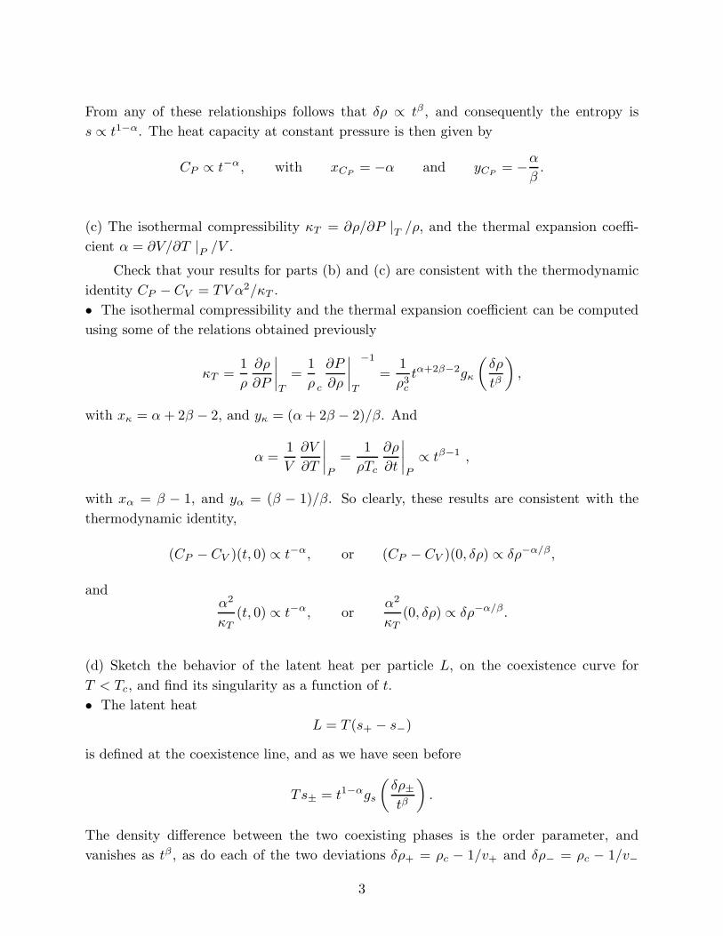
(d) Sketch the behavior of the latent heat per particle L, on the coexistence curve for

T < Tc, and find its singularity as a function of t.

• The latent heat L = T (s+ − s−)

is defined at the coexistence line, and as we have seen before

δρ±Ts± = t1−α gs .

tβ

The density difference between the two coexisting phases is the order parameter, and

vanishes as tβ , as do each of the two deviations δρ+ = ρc − 1/v+ and δρ− = ρc − 1/v−

3

( )

( )

∣

∣

∣

∣

∣

∣

∣

∣

∣

∣

∣

∣

∣

∣

∣

∣

L

t t=0

of the gas and liquid densities from the critical critical value. (More precisely, as seen in

(b), δρ|P=constant ∝ tβ.) The argument of g in the above expression is thus evaluated at

a finite value, and since the latent heat goes to zero on approaching the critical point, we

get

L ∝ t1−α , with xL = 1− α.

********

2. The Ising model: The differential recursion relations for temperature T , and magnetic

field h, of the Ising model in d = 1 + ǫ dimensions are dT T 2

dℓ = − ǫ T +

2 ,

dh =dh .

dℓ

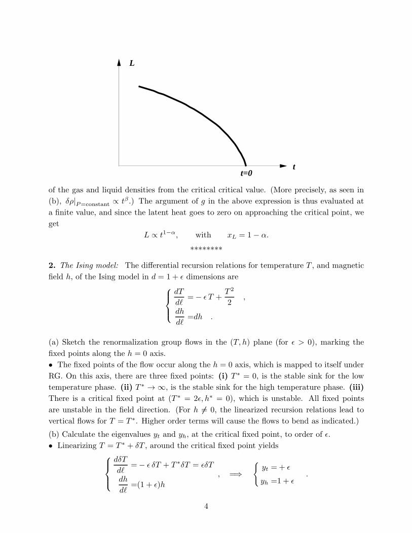
(a) Sketch the renormalization group flows in the (T, h) plane (for ǫ > 0), marking the

fixed points along the h = 0 axis.

• The fixed points of the flow occur along the h = 0 axis, which is mapped to itself under

RG. On this axis, there are three fixed points: (i) T ∗ = 0, is the stable sink for the low

temperature phase. (ii) T ∗ → ∞, is the stable sink for the high temperature phase. (iii) There is a critical fixed point at (T ∗ = 2ǫ, h∗ = 0), which is unstable. All fixed points

are unstable in the field direction. (For h �= 0, the linearized recursion relations lead to

vertical flows for T = T ∗ . Higher order terms will cause the flows to bend as indicated.)

(b) Calculate the eigenvalues yt and yh, at the critical fixed point, to order of ǫ.

• Linearizing T = T ∗ + δT , around the critical fixed point yields dδT

= − ǫ δT + T ∗ δT = ǫδT yt =+ ǫdℓ , =⇒ . dh yh =1 + ǫ=(1 + ǫ)h

dℓ

4

6

{

(c) Starting from the relation governing the change of the correlation length ξ under

t−ν( )

renormalization, show that ξ(t, h) = gξ h/|t|Δ (where t = T/Tc − 1), and find the exponents ν and Δ.

• Under rescaling by a factor of b, the correlation length is reduced by b, resulting in the

homogeneity relation

ξ(t, h) = bξ(bytt, byhh).

Upon selecting a rescaling factor such that bytt ∼ 1, we obtain (

−νξ(t, h) = t gξ h/|t|Δ) ,

with 1 1 yh 1

ν = = , and Δ = = + 1. yt ǫ yt ǫ

(d) Use a hyperscaling relation to find the singular part of the free energy fsing.(t, h), and hence the heat capacity exponent α.

• According to hyperscaling

(

d/ytfsing.(t, h) ∝ ξ(t, h)−d = t gf h/|t|Δ) .

Taking two derivatives with respect to t leads to the heat capacity, whose singularity for h = 0 is described by the exponent

1 + ǫ α = 2− dν = 2− = − + 1.

ǫ ǫ 1

5

(e) Find the exponents β and γ for the singular behaviors of the magnetization and sus­

ceptibility, respectively.

• The magnetization is obtained from the free energy by

∂f d − yh m = − ∼ |t|β , with β = = 0.

∂h yth=0

(There will be corrections to β at higher orders in ǫ.) The susceptibility is obtained from

a derivative of the magnetization, or

∂2f 2yh − d 1 + ǫ 1 χ = − ∼ |t|−γ , with γ = = = + 1.

∂h2 yt ǫ ǫh=0

(f) Starting the relation between susceptibility and correlations of local magnetizations,

calculate the exponent η for the critical correlations ((m(0)m(x)) ∼ |x|−(d−2+η)).

• The magnetic susceptibility is related to the connected correlation function via

χ = dd x (m(0)m(x)) . c

Close to criticality, the correlations decay as a power law (m(0)m(x)) ∼ |x|−(d−2+η), which

is cut off at the correlation length ξ, resulting in

χ ∼ ξ(2−η) ∼ |t|−(2−η)ν .

From the corresponding exponent identity, we find

γ = (2− η)ν, =⇒ η = 2− ytγ = 2− 2yh + d = 2− d = 1− ǫ.

(g) How does the correlation length diverge as T → 0 (along h = 0) for d = 1?

• For d = 1, the recursion relation for temperature can be rearranged and integrated, i.e.

1 dT 1 2 = , =⇒ d − = dℓ.

T 2 dℓ 2 T

We can integrate the above expression from a low temperature with correlation length

ξ(T ) to a high temperature where 1/T ≈ 0, and at which the correlation length is of the order of the lattice spacing, to get

2 ξ 2 = ln =⇒ ξ(T ) = a exp .

T a T

6

∣

∣

∣

∣

∣

∣

∣

∣

( )

( ) ( )

********

3. Longitudinal susceptibility: While there is no reason for the longitudinal susceptibility

to diverge at the mean-field level, it in fact does so due to fluctuations in dimensions d < 4.

This problem is intended to show you the origin of this divergence in perturbation theory.

There are actually a number of subtleties in this calculation which you are instructed to

ignore at various steps. You may want to think about why they are justified.

Consider the Landau–Ginzburg Hamiltonian:

K=

tβH dd x

(2

∇mm )2 + mm 2 + u(mm 2 )2

,2

describing an n–component magnetization vector mm (x), in the ordered phase for t < 0.

m(a) Letmm (x) = (

m+φℓ(x))

eℓ+φt(x)et, and expand βH keeping all terms in the expansion.

• With mm m(x) = (m+ φℓ (x)) eℓ + φt (x) et, and m the minimum of βH,

β

(

t+ um

)

+

dd x

{

K

22 4 tH =V m (

2 2∇ 2 mφ ) +

(

∇φ)

+

(

+ 6um2

)

2 ℓ t

2

φℓ

(

¯

) t 22 m m m m+ + 2um φ 2

t + 4um(

φ3 ℓ + φℓφ2

t

)

+ u

φ4 ℓ + 2φ2ℓφ2

t + φ 2t

�

.2

( )

Since m2 = −t/4u in the ordered phase (t < 0), this expression can be simplified, upon

dropping the constant term, as

{

Kβ

( 2 H 2 2 3 m= dd

x

(∇φ 2ℓ + ∇m) φt

tφ 42

)

− ℓ + um

(

φℓ + φℓφt

)

2

+u

φ4 mℓ + 2φ2mℓ φ

2t +

(

φ 2t

)

�

.

m(b) Regard the quadratic terms in φℓ and φt as an unperturbed Hamiltonian βH0, and the mlowest order term coupling φℓ and φt as a perturbation U ; i.e.

U = 4um

d md xφℓ(x)φt(x)2 .

Write U min Fourier space in terms of φℓ(q) and φt(q).

• We shall focus on the cubic term as a perturbation

= 4um

dd m 2U xφℓ (x)φt (x) ,

7

�

� �

which can be written in Fourier space as

′ ddq ddqU = 4um φℓ (−q − q ′ )φmt (q) · φmt (q ′ ) .

d d(2π) (2π)

(c) Calculate the Gaussian (bare) expectation values (φℓ(q)φℓ(q ′ ))0 and (φt,α(q)φt,β(q ′ ))0, and the corresponding momentum dependent susceptibilities χℓ(q)0 and χt(q)0.

• From the quadratic part of the Hamiltonian,

( )22

βH0 = dd x 1

K (∇φℓ) + ∇φmt − 2tφ2 ,ℓ2

we read off the expectation values

d

(2π) δd (q + q ′ ) (φℓ (q)φℓ (q ′ ))0 = Kq2 − 2t

,d

δd (q + q (2π) ′ ) δαβ (φt,α (q)φt,β (q ′ )) = 0 Kq2

and the corresponding susceptibilities

1

χℓ (q)0 =

Kq2 − 2t .

1 χt (q)0 =

Kq2

m ′ m ′ (d) Calculate (φmt(q1) · φt(q2) φmt(q1) · φt(q2))0 using Wick’s theorem. (Don’t forget that mφt is an (n − 1) component vector.)

• Using Wick’s theorem,

( )

m m m ′ m ′ ′ ′ φt (q1) · φt (q2)φt (q1) · φt (q2) ≡ (φt,α (q1)φt,α (q2)φt,β (q1)φt,β (q2))00

′ ′ ′ ′ = (φt,α (q1)φt,α (q2)) (φt,β (q1)φt,β (q2)) + (φt,α (q1)φt,β (q1)) (φt,α (q2)φt,β (q2))0 0 0 0

′ ′ + (φt,α (q1)φt,β (q2)) (φt,α (q2)φt,β (q1)) .0 0

Then, from part (c),

2d ( ) ′ ′ (2π) 2 δ

d (q1 + q2) δd (q1 + q2)m m m ′ m ′ φt (q1) · φt (q2)φt (q1) · φt (q2) = (n − 1)

K2 2 ′20 q1q1

′ ′ ′ ′ δd (q1 + q1) δd (q2 + q2) δd (q1 + q2) δ

d (q1 + q2)+ (n − 1) + (n − 1) ,2 2 2 2q q1q2 1q2

8

∫

∫

{

}

[ ]

� � � ( )�

� �

2since δααδββ = (n − 1) , and δαβδαβ = (n − 1).

(e) Write down the expression for (φℓ(q)φℓ(q ′ )) to second-order in the perturbation U .

Note that since U is odd in φℓ, only two terms at the second order are non–zero.

• Including the perturbation U in the calculation of the correlation function, we have

−Uφℓ (q)φℓ (q ′ ) e φℓ (q)φℓ (q ′ ) 1− U + U2/2 + · · ·0 0(φℓ (q)φℓ (q ′ )) = = . (e−U )0 ((1− U + U2/2 + · · ·))0

Since U is odd in φℓ, (U)0 = (φℓ (q)φℓ (q ′ )U)0 = 0. Thus, after expanding the denomina­

tor to second order,

1 U2 (

U3)

= 1− + O ,1 + (U2/2)0 + · · · 2 0

we obtain

(φℓ (q)φℓ (q ′ )) = (φℓ (q)φℓ (q ′ ))0 +1 (�

φℓ (q)φℓ (q ′ )U2�

− (φℓ (q)φℓ (q ′ ))0 � U2

� ) .

0 02

(f) Using the form of U in Fourier space, write the correction term as a product of two

4–point expectation values similar to those of part (d). Note that only connected terms

for the longitudinal 4–point function should be included.

• Substituting for U its expression in terms of Fourier transforms from part (b), the

fluctuation correction to the correlation function reads

GF (q, q ′ ) ≡ (φℓ (q)φℓ (q ′ )) − (φℓ (q)φℓ (q ′ ))0 dd dd dd ′ dd ′ (1 2 q1 q2 q q21 m m= (4um) φℓ (q)φℓ (q ′ )φℓ (−q1 − q2)φt (q1) · φt (q2)d d d d2 (2π) (2π) (2π) (2π)

) 1′ ′ m ′ m ′ � U2

� × φℓ (−q1 − q2)φt (q1) · φt (q2) − (φℓ (q)φℓ (q ′ ))0 ,

00 2

i.e. GF (q, q ′ ) is calculated as the connected part of

′ ′ 1 2 ddq1 ddq2 d

dq ddq2 ′1 ′ (4um) (φℓ (q)φℓ (q ′ )φℓ (−q1 − q2)φℓ (−q1 − q2))0d d d d2 (2π) (2π) (2π) (2π)( )

m m ′ ′ m m× φt (q1) · φt (q2)φt (q1) · φt (q2) , 0

where we have used the fact that the unperturbed averages of products of longitudinal and

9

∫

∫

�

�

�

�

transverse fields factorize. Hence

′ )1 2 ddq1 d

dq2 ddq1

′ ddq2 ′ (

m m m ′ m ′ )

GF (q, q = (4um) φt (q1) · φt (q2)φt (q1) · φt (q2)d d d d2 (2π) (2π) (2π) (2π) 0

′ ′ × (φℓ (q)φℓ (−q1 − q2))0 (φℓ (q ′ )φℓ (−q1 − q2))0 ′ ′ + (φℓ (q)φℓ (−q1 − q2))0 (φℓ (q ′ )φℓ (−q1 − q2))0

dd dd dd ′ dd ′ ( )1 2 q1 q2 q q2 ′1 ′ m m m m= 2× (4um) φt (q1) · φt (q2)φt (q1) · φt (q2)d d d d2 (2π) (2π) (2π) (2π) 0

′ ′ × (φℓ (q)φℓ (−q1 − q2))0 (φℓ (q ′ )φℓ (−q1 − q2))0 .

Using the results of parts (c) and (d) for the two and four points correlation functions, 2 2and since u m = −ut/4, we obtain

dd dd dd ′ dd ′ 2d ′ ′ q1 q2 q q (2π) 2 δd (q1 + q2) δ

d (q1 + q2)1 2GF (q, q ′ ) = 4u (−t) (n − 1)d d d d K2 q2 ′2

(2π) (2π) (2π) (2π) 1q1

′ ′ ′ ′ δd (q1 + q1) δd (q2 + q2) + δd (q1 + q2) δ

d (q1 + q2)+ (n − 1) 2 2q1q2

d d ′ ′ ′ (2π) δd (q − q1 − q2) (2π) δd (q − q1 − q2)× ,Kq2 − 2t Kq2 − 2t

which, after doing some of the integrals, reduces to

2 4u (−t) 2 δ

d (q) δd (q ′ ) ddq1GF (q, q ′ ) = (n − 1)

K2 24t2 q1

δd (q + q ′ ) ddq1+ 2 (n − 1) .2 22(Kq2 − 2t) q (q + q1)1

(g) Ignore the disconnected term obtained in (d) (i.e. the part proportional to (n − 1)2),

and write down the expression for χℓ(q) in second order perturbation theory.

• From the dependence of the first term (proportional to δd (q) δd (q ′ )), we deduce that

this term is actually a correction to the unperturbed value of the magnetization, i.e.

2(n − 1)u ddq1 m → m 1− 2 ,

Kt q1

and does not contribute to the correlation function at non-zero separation. The spatially

varying part of the connected correlation function is thus

d(2π) δd (q + q ′ ) 8u (−t) δd (q + q ′ ) ddq1(φℓ (q)φℓ (q ′ )) = + (n − 1) 2 ,2Kq2 − 2t K2 (Kq2 − 2t) q2 (q + q1)1

10

[ (∫

)]

∫

{

(∫

)

∫

}

∫

∫

∫

{

}

leading to

1 8u (−t) (n − 1) ddq1 1 χℓ (q) = + .

K2 2 d 2 2Kq2 − 2t (Kq2 − 2t) (2π) q (q + q1)1

(h) Show that for d < 4, the correction term diverges as qd−4 for q → 0, implying an

infinite longitudinal susceptibility.

• In d > 4, the above integral converges and is dominated by the large q cutoff Λ. In

d < 4, on the other hand, the integral clearly diverges as q → 0, and is thus dominated ′ by small q1 values. Changing the variable of integration to q = q1/q, the fluctuation 1

correction to the susceptibility reads

Λ/q ′ ∞ ′ ddq 1 ddq 1 (

0)

d−4 1 d−4 1χℓ (q)F ∼ q = q + O q ,2d ′2 ′ d ′2 ′ 2 0 (2π) q (q+ q ) 0 (2π) q (q+ q )1 1 1 1

which diverges as qd−4 for q → 0. NOTE: For a translationally invariant system,

(φ (x)φ (x ′ )) = ϕ (x − x ′ ) ,

which implies

′ iq·x+iq ·x(φ (q)φ (q ′ )) = ddxdd x e ′ ′ (φ (x)φ (x ′ ))

′ )+i(q+q ′ ′ iq·(x−x ′ )·x = dd (x − x ′ ) dd x e ϕ (x − x ′ )

d = (2π) δd (q + q ′ )ψ (q) .

Consider the Hamiltonian

ddq−βH ′ = −βH + ddxh (x)φ (x) = −βH + h (q)φ (−q) ,d

(2π)

where −βH is a translationally invariant functional of φ (a one-component field for sim­

plicity), independent of h (x). We have

ddq m (x = 0) = (φ (0)) = (φ (q)) ,

d(2π)

and, taking a derivative,

′ ∂m ddq = (φ (q ′ )φ (q)) .

d∂h (q) (2π)

11

∫

∫ ∫

∫

∫

∫ ∫

∫

∫

At h = 0, the system is translationally invariant, and

∂m ∂h (q)

∣

∣

∣

∣

= ψ (q) . h=0

Also, for a uniform external magnetic field, the system is translationally invariant, and

−βH ′ = −βH + h

∫

ddxφ (x) = −βH + hφ (q = 0) ,

yielding ∂m ddq ′

χ = = φ (q′ )φ (q = 0) = ψ (0) .∂h

∫

d(2π)

( )

********

4. Crystal anisotropy: Consider a ferromagnet with a tetragonal crystal structure. Cou­

pling of the spins to the underlying lattice may destroy their full rotational symmetry. The

resulting anisotropies can be described by modifying the Landau–Ginzburg Hamiltonian

to K

βH ∫

[

2 = dd x (∇mm )2 t

+ mm 2 r + u mm 2 + m2 + v m2mm 2 ,

2 2

( )

2 1 1

]

w · n

here mm ≡ (m1, · · , mn), andmm2 =

L

2i=1 mi (d = n = 3 for magnets in three dimensions).

Here u > 0, and to simplify calculations we shall set v = 0 throughout.

(a) For a fixed magnitude |mm |; what directions in the n component magnetization space

are selected for r > 0, and for r < 0? • r > 0 discourages ordering along direction 1, and leads to order along the remaining

(n − 1) directions.

r < 0 encourages ordering along direction 1.

(b) Using the saddle point approximation, calculate the free energies (lnZ) for phases

uniformly magnetized parallel and perpendicular to direction 1.

• In the saddle point approximation for mm (x) = me1, we have [

t + r lnZ 2 4

sp = −V min m + um ,2

]

m

where V = J

ddx, is the system volume. The minimum is obtained for

3

�{

0 for t + r > 0(t + r)m + 4um = 0, =⇒ m = .−(t + r)/4u for t + r < 0

For t + r < 0, the free energy is given by

J

lnZ p t + r)2 s (fsp = − = − .

V 16u

12

�

� �

When the magnetization is perpendicular to direction 1, i.e. for mm(x) = mˆ � 1, theei for i =

corresponding expressions are

t 0 for t > 02 4 3 JlnZsp = −V min m + um , tm + 4um = 0, m = ,

2 −t/4u for t < 0 m

and the free energy for t < 0 is t2

fsp = − . 16u

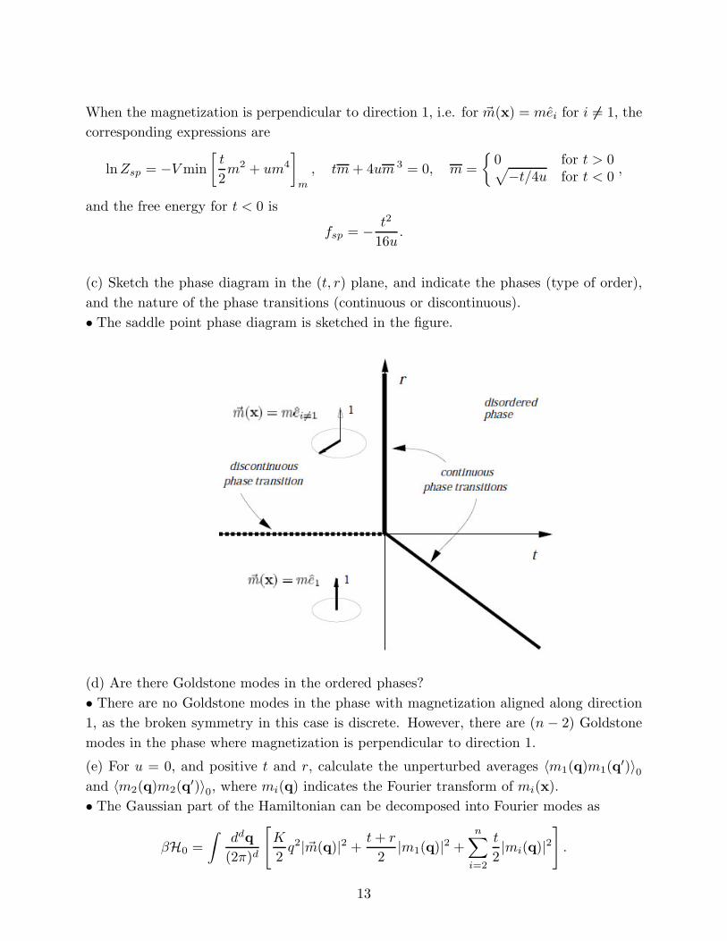
(c) Sketch the phase diagram in the (t, r) plane, and indicate the phases (type of order),

and the nature of the phase transitions (continuous or discontinuous).

• The saddle point phase diagram is sketched in the figure.

(d) Are there Goldstone modes in the ordered phases?

• There are no Goldstone modes in the phase with magnetization aligned along direction

1, as the broken symmetry in this case is discrete. However, there are (n − 2) Goldstone

modes in the phase where magnetization is perpendicular to direction 1.

(e) For u = 0, and positive t and r, calculate the unperturbed averages (m1(q)m1(q ′ ))0 and (m2(q)m2(q ′ ))0, where mi(q) indicates the Fourier transform of mi(x).

• The Gaussian part of the Hamiltonian can be decomposed into Fourier modes as

ndd �q K t + r t

βH0 = q 2|mm(q)|2 + |m1(q)|2 + |mi(q)|2 . (2π)d 2 2 2

i=2

13

6

[ ] {

∫

�

�

� �

�

�

�

�

�

�

�

From this form we can easily read off the covariances

(2π)dδd(q + q

(m1(q)m1(q ′ ))0 =

′ )

t + r + Kq2 .

(2π)dδd(q + q ′ ) (m2(q)m2(q ′ ))0 =

t + Kq2

J (f) Write the fourth order term U ≡ u ddx(mm2)2, in terms of the Fourier modes mi(q).

J dd

q• Substituting mi(x) = exp(iq · x)mi(q) in the quartic term, and integrating over(2π)d

x yields

n (

2)2 ddq1d

dq2ddq3U = u dd x mm = u mi(q1)mi(q2)mj(q3)mj(−q1 − q2 − q3).

(2π)3d i,j=1

(g) Treating U as a perturbation, calculate the first order correction to (m1(q)m1(q ′ )). (You can leave your answers in the form of some integrals.)

• In first order perturbation theory (O) = (O)0 − ((OU)0 − (O)0 (U)0), and hence n

ddq1ddq2d

dq3(m1(q)m1(q ′ )) = (m1(q)m1(q ′ ))0 − u (2π)3d

i,j=1 ( )c(m1(q)m1(q ′ )mi(q1)mi(q2)mj(q3)mj(−q1 − q2 − q3))0

(2π)dδd(q + q ′ ) u ddk 4(n − 1) 4 8 = 1− + +

t + r + Kq2 t + r + Kq2 (2π)d t + Kk2 t + r + Kk2 t + r + Kk2

The last result is obtained by listing all possible contractions, and keeping track of how

many involve m1 versus mi�=1. The final result can be simplified to

(2π)dδd(q + q ′ ) 4u ddk n − 1 3 (m1(q)m1(q ′ )) = 1− + t + r + Kq2 t + r + Kq2 (2π)d t + Kk2 t + r + Kk2

(h) Treating U as a perturbation, calculate the first order correction to (m2(q)m2(q ′ )). • Similar analysis yields

nddq1d

dq2ddq3(m2(q)m2(q ′ )) = (m2(q)m2(q ′ ))0 − u

(2π)3d i,j=1

( )c(m2(q)m2(q ′ )mi(q1)mi(q2)mj(q3)mj(−q1 − q2 − q3))0(2π)dδd(q + q ′ ) u ddk 4(n − 1) 4 8

= 1− + + t + Kq2 t + Kq2 (2π)d t + Kk2 t + r + Kk2 t + Kk2

(2π)dδd(q + q ′ ) 4u ddk n + 1 1 = 1− + .

t + Kq2 t + Kq2 (2π)d t + Kk2 t + r + Kk2

14

∫ ∫

∫

{ ∫ [ ]}

6

{∫

[ ]}

{∫

]

{∫

}

6

∫

[ ]

[ ]

∑

∑

6

∑

6

}

�

�

�

�

�

(i) Using the above answer, identify the inverse susceptibility χ−1 22 , and then find the

transition point, tc, from its vanishing to first order in u.

• Using the fluctuation–response relation, the susceptibility is given by

χ22 = dd x (m2(x)m2(0)) = ddq (m2(q)m2(q = 0))(2π)d

1 4u ddk n + 1 1 = 1− + . t t (2π)d t + Kk2 t + r + Kk2

Inverting the correction term gives

ddk n + 1 1 χ−1 = t + 4u + + O(u 2).22 (2π)d t + Kk2 t + r + Kk2

The susceptibility diverges at

ddk n + 1 1 tc = −4u + + O(u 2).

(2π)d Kk2 r + Kk2

(j) Is the critical behavior different from the isotropic O(n) model in d < 4? In RG

language, is the parameter r relevant at the O(n) fixed point? In either case indicate the

universality classes expected for the transitions.

• The parameter r changes the symmetry of the ordered state, and hence the universality

class of the disordering transition. As indicated in the figure, the transition belongs to

the O(n − 1) universality class for r > 0, and to the Ising class for r < 0. Any RG

transformation must thus find r to be a relevant perturbation to the O(n) fixed point.

********

5. Cubic anisotropy– Mean-field treatment: Consider the modified Landau–Ginzburg

Hamiltonian

n 2 4βH = dd x

K (∇mm)2 +

tmm + u(mm 2)2 + v m ,i2 2

i=1

for an n–component vector mm(x) = (m1, m2, · · · , mn). The “cubic anisotropy” term n 4

i , breaks the full rotational symmetry and selects specific directions.i=1 m

(a) For a fixed magnitude |mm|; what directions in the n component magnetization space

are selected for v > 0 and for v < 0? What is the degeneracy of easy magnetization axes

in each case?

15

L

∫ ∫

{∫

[ ]}

]

∫[ ]

∫

[

∑

]

∫[

^2

e e2 m m m m

m m

mm

^1

e e 1

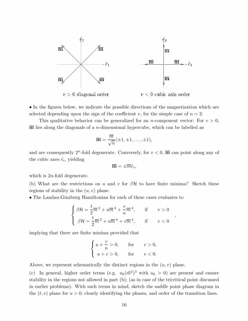
�v 0 diagonal order �v 0 cubic axis order

• In the figures below, we indicate the possible directions of the magnetization which are

selected depending upon the sign of the coefficient v, for the simple case of n = 2:

This qualitative behavior can be generalized for an n-component vector: For v > 0,

m lies along the diagonals of a n-dimensional hypercube, which can be labelled as

m m = √ (±1, ±1, . . . , ±1),

n

and are consequently 2n-fold degenerate. Conversely, for v < 0, m can point along any of

the cubic axes ei, yielding

m = ±mei,

which is 2n-fold degenerate.

(b) What are the restrictions on u and v for βH to have finite minima? Sketch these

regions of stability in the (u, v) plane. • The Landau-Ginzburg Hamiltonian for each of these cases evaluates to

t v

2 4 4 βH = m + um + m , if v > 0

2 n t

, 2 4 4βH = m + um + vm , if v < 0

2

implying that there are finite minima provided that

v u + > 0, for v > 0,

n u + v > 0, for v < 0.

Above, we represent schematically the distinct regions in the (u, v) plane.

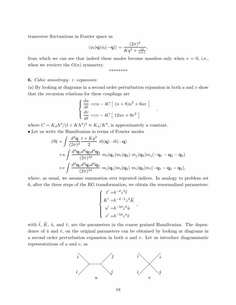
(c) In general, higher order terms (e.g. u6(mm2)3 with u6 > 0) are present and ensure

stability in the regions not allowed in part (b); (as in case of the tricritical point discussed

in earlier problems). With such terms in mind, sketch the saddle point phase diagram in

the (t, v) plane for u > 0; clearly identifying the phases, and order of the transition lines.

16

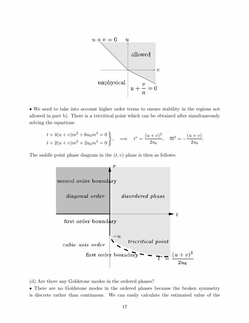
nunphysicalu+ v = 0 allowed

u+ v = 0u v

• We need to take into account higher order terms to ensure stability in the regions not

allowed in part b). There is a tricritical point which can be obtained after simultaneously

solving the equations

t+ 4(u+ v)m2 + 6u6m4 = 0

}

, =⇒ t∗(u+ v)2 )

= , 2 (u+ vm = .

t+ 2(u+ v)m2 + 2u6m4 = 0 2u6

−2u6

The saddle point phase diagram in the (t, v) plane is then as follows:

(d) Are there any Goldstone modes in the ordered phases?

• There are no Goldstone modes in the ordered phases because the broken symmetry

is discrete rather than continuous. We can easily calculate the estimated value of the

17

transverse fluctuations in Fourier space as

(2π)d〈φt(q)φt(−q)〉 = vt ,Kq2 + u+v

from which we can see that indeed these modes become massless only when v = 0, i.e.,

when we retrieve the O(n) symmetry.

********

6. Cubic anisotropy– ε–expansion:

(a) By looking at diagrams in a second order perturbation expansion in both u and v show

that the recursion relations for these couplings are

du

=εu− 4C[

(n+ 8)u2 + 6uvdℓ ,

dv=εv − 4C 12uv + 9v2

]

dℓ

where C = KdΛd/(t+KΛ2)2 ≈ K4/K

2, i

[

s approximat

]

ely a constant.

• Let us write the Hamiltonian in terms of Fourier modes

βH =

∫

ddq t+Kq2m~ (q) ·m~ (

(2π)d 2−q)

∫

ddq dd d1 q2d q3

+u mi(q1)mi(q2) mj(q3)mj(−q1 − q2(2π)3d

− q3)

ddq1ddq2d

dq3+v

∫

mi(q1)mi(q2) mi(q3)mi((2π)3d

−q1 − q2 − q3),

where, as usual, we assume summation over repeated indices. In analogy to problem set

6, after the three steps of the RG transformation, we obtain the renormalized parameters:

t′ =b−dz2t

i

K ′ =b−d−2z2K,

u′ =

jb−3dz4u

˜ ˜

v′ =b−3dz4v

with t, K, u, and v, are

ithe param

eters

jin the coarse

iigrained Hamiltonian. The depen-

dence of u and v, on the original

uparameters can be obtained by looking at diagrams in

a second order perturbation expansion in both u and v. Let us introduce diagrammatic

representations of u and v, as iv i18

q2 iq1 + q2l� q q4 2�2�4�2u22 (t+KKd��d2)2 �lq1 i q j q3q2 mq1 + q2 �l q q4 4� 4� 2u22 (t+KKd��d2)2 �lq1 ii q jj q3 2� 6� 2uv (t+KKd��d2)2 �lq2 i lq1 + q2 � q q4 (t+K� )

qq1 + q2 � q q4q1q2q1 i q j q3 q1 i q j q3 6� 4� 2uv Kd�d2 2 �lq2 q + q � q1 2 q4where, again we have set b = eδℓ. The new coarse grained parameters are

{

u = u− 4C[(n+ 8)u2 + 6uv]δℓ,

v = v − 4C[9v2 + 12uv]δℓ

which after introducing the parameter ǫ = 4 − d, rescaling, and renormalizing, yield the

recursion relations

du

=ǫu− 4C[(n+ 8)u2 + 6uv]dℓ .

dv=ǫv − 4C[9v2 + 12uv]

dℓ

(b) Find all fixed points in the (u, v) plane, and draw the flow patterns for n < 4 and

n > 4. Discuss the relevance of the cubic anisotropy term near the stable fixed point in

each case.

• From the recursion relations, we can obtain the fixed points (u∗, v∗). For the sake of

simplicity, from now on, we will refer to the rescaled quantities u = 4Cu, and v = 4Cv, in

terms of which there are four fixed points located at

u∗ = v∗ = 0 Gaussian fixed point

ǫu∗ = 0 v∗ = Ising fixed point

9.u∗

ǫ= v∗ = 0 O(n) fixed point

(n+ 8)

∗ ǫ ∗ ǫ(nu = v =

− 4)Cubic fixed point

3n 9n

q3i ji j Contributions to vqq1 + q2 � qq1q2 q4q3ii jjContributions to u 2� 2� 2nu22 Kd�d(t+K�2)2 �l 6� 6� 2v22 Kd�d(t+K�2)2 �l

19

Linearizing the recursion relations in the vicinity of the fixed point gives

∗d δu ǫ 2(n+ 8)u 6v∗ 6u∗ δu

A =d

(

δv

)

=− − −

.ℓ

∗ ∗

(

−12v∗ ǫ− 12u∗ − 18v∗,v

)(

δvu

)

As usual, a positive eigenvalue corresponds to an unstable direction, whereas negative ones

correspond to stable directions. For each of the four fixed points, we obtain:

1. Gaussian fixed point: λ1 = λ2 = ǫ, i.e., this fixed point is doubly unstable for ǫ > 0, as

A =

(

ǫ 0

0 ǫ

)

.

2. Ising fixed point: This fixed point has one stable and one unstable direction, as

ǫ0

3A = ǫ−43

− ǫ

,

corresponding to λ1 = ǫ/3 and λ2 = −ǫ. Note that for u = 0, the system decouples into n

noninteracting 1-component Ising spins.

3. O(n) fixed point: The matrix

A =

ǫ−ǫ − 6 (n+ 8)

,(n− 4)

0 ǫ(n+ 8)

has eigenvalues λ1 = −ǫ, and λ2 = ǫ(n − 4)/(n+ 8). Hence for n > 4 this fixed point has

one stable an one unstable direction, while for n < 4 both eigendirections are stable. This

fixed point thus controls the critical behavior of the system for n < 4.

4. Cubic fixed point: The eigenvalues of

A =

(n+ 8)−

3− 2 ǫ

,

(n− 4)4 4

3− n

n−

are λ1 = ǫ(4 − n)/3n, λ2 = −ǫ. Thus for n < 4, this fixed point has one stable and one

unstable direction, and for n > 4 both eigendirections are stable. This fixed point controls

critical behavior of the system for n > 4.

20

u

vn<4

u

v n> 4

q q2q1q1q2ii i jq

q1q ii q2~t = t+4 Kd�d(t+K�2)[(n+2)u+3v]dtdl = 2t+4 Kd�d(t+K�2) [(n+2)u+3v]

2nu Kd�d(t+K�2)�l4u Kd�d(t+K�2)�l6v Kd�d(t +K�2)�l

In the (u,v) plane, v∗ = 0 for n < 4, and the cubic term is irrelevant, i.e., fluctuations

restore full rotational symmetry. For n > 4, v is relevant, resulting in the following flows:

(c) Find the recursion relation for the reduced temperature, t, and calculate the exponent

ν at the stable fixed points for n < 4 and n > 4.

• Up to linear order in ǫ, the following diagrams contribute to the determination of t:

After linearizing in the vicinity of the stable fixed points, the exponent yt is given by

yt = 2− 4C[(n+ 2)u∗ + 3v∗],=⇒ ν =1

yt=

1

2+

(n+ 2)

4(n+ 8)ǫ+O(ǫ2) for n < 4

1

2+

(n− 1)

6nǫ+O(ǫ2) for n > 4

.

(d) Is the region of stability in the (u, v) plane calculated in part (b) of the previous

problem enhanced or diminished by inclusion of fluctuations? Since in reality higher order

terms will be present, what does this imply about the nature of the phase transition for a

small negative v and n > 4?

• All fixed points are located within the allowed region calculated in 1b). However, not

all flows starting in classically stable regions are attracted to stable fixed point. If the RG

21

flows take a point outside the region of stability, then fluctuations decrease the region of

stability. The domains of attraction of the fixed points fo

ysicalr n <

domainunph4 and n >

of4

vare indicated

in the following figures: attractionu+n n = 0> 4 v

Flows which are not originally located within these domains of attraction flow into

the unphysical regions. The coupling constants u and v become more negative. This is

the signal of a fluctuation induced first order phase transition, by what is known as the

Coleman–Weinberg mechanism. Fluctuations are responsible for the change of order of the

transition in the regions of the (u,v) plane outside the domain of attraction of the stable

fixed points.

********

7. Cumulant method: Apply the Niemeijer–van Leeuwen first order cumulant expansion

to the Ising model on a square lattice with −βH = K <ij> σiσj , by following these steps:

(a) For an RG with b = 2, divide the bonds into intra–

∑

cell components βH0; and inter–cell

components U .• The N sites of the square lattice are partitioned into N/4 cells as indicated in the

figure below (the intra-cell and inter-cell bonds are represented by solid and dashed lines

respectively).

The renormalized Hamiltonian βH′[σ′α] is calculated from

βH′ [σ′ 1 2α] = − lnZ0 [σ

′α] + 〈U〉0 − 2

(

⟨

U2⟩

0− 〈U〉0

)

+O(

U3)

,

where 〈〉0 indicates expectation values calculated with the weight exp(−βH0) at fixed [σ′α].

(b) For each cell α, define a renormalized spin σ′α = sign(σ1

α + σ2 3 4α + σα + σα). This choice

4becomes ambiguous for configurations such that

∑

ii=1 σα = 0. Distribute the weight of

these configurations equally between σ′α = +1 and −1 (i.e. put a factor of 1/2 in addition

22

u+ v = 0 u

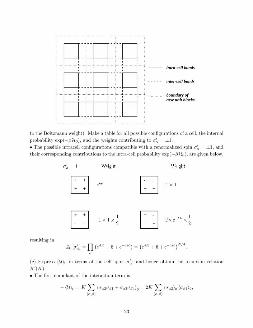
intra-cell bonds

inter-cell bonds

boundary ofnew unit blocks

to the Boltzman

�n

�weight). Make a table for all possible configurations of a cell, the internal

probability exp(−βH0), and the weights contributing to σ′α = ±1.

• The possible intracell configurations compatible with a renormalized spin σ′α = ±1, and

their correspondin0 g=co1ntribution Weighte4s

Kto the intra-cell probability exp Weigh0t

4�(−

1βH ), are given below,

+ + +

1� 1-

+ +

4� 2+ +

+ + + -

- - - +2�e�4K� 21

resulting in/4

Z [σ′ ] =∏

( Ne4K0 α + 6 + e−4K

)

=(

e4K + 6 + e−4K

α

)

.

(c) Express 〈U〉0 in terms of the cell spins σ′α; and hence obtain the recursion relation

K ′(K).

• The first cumulant of the interaction term is

−〈U〉0 = K∑

〈σα2σβ1 + σα3σβ4〉 = 2K0

〈α,β〉 〈

∑

〈σα2〉0 〈σβ1〉0,α,β〉

23

- - e4K + -

- -4� 1

+ +

- -4� 1� 12

- -

+ -

- +2�e�4K� 21

1 2 1 2

α β

4 3 4 3

where, for σ′α = 1,

e4K + (3 1) + 0 + 0 e4K + 2〈σαi−〉0 = = .

(e4K + 6 + e−4K) (e4K + 6 + e−4K)

Clearly, for σ′α = −1 we obtain the same result with a global negative sign, and thus

′ e4K + 2〈σαi〉0 = σα .(e4K + 6 + e−4K)

As a result,

2N 4K

−βH′ [σ′α] = ln

4

(

4 ee K + 6 + e−4K

)

+ 2K

(

+ 2σ′ σ′ ,

e4K + 6 + e−4K

)

α β

〈

∑

α,β〉

corresponding to the recursion relation K ′(K),

24K′

(

e + 2K = 2K

e4K + 6 + e−4K

)

.

(d) Find the fixed point K∗, and the thermal eigenvalue yt.

• To find the fixed point with K ′ = K = K∗, we introduce the variable x = e4K∗

. Hence,

we have to solve the equation

x+ 2 1= √ , or

√x+ 6 + x−1 2

(

2− 1)

x2 −(

6− 2√2)

x− 1 = 0,

24

Weight Weight�0� = �1

whose only meaningful solution is x ≃ 7.96, resulting in K∗ ≃ 0.52.

To obtain the thermal eigenvalue, let us linearize the recursion relation around this

non-trivial fixed point,

∂K ′∣

K∗ ∗

∣

4 4K∗ −4K∣ = byt

e, y e e⇒ 2 t = 1 + 8K∗ −

, y 1.00 .∂K K∗

[

∣

t 6e4K∗ + 2

−e4K∗ + 6 + e−4K∗

]

⇒ ≃

(e) In the presence of a small magnetic field h∑

i σi , find the recursion relation for h; and

calculate the magnetic eigenvalue yh at the fixed point.

• In the presence of a small magnetic field, we will have an extra contribution to the

Hamiltonian

h∑ e4K + 2〈σ ′

α,i〉0 = 4h σ .(e4K + 6 + e−4K)

α,

∑

α

i α

Therefore,

′ e4K + 2h = 4h .

(e4K + 6 + e−4K)

(f) Compare K∗, yt, and yh to their exact values.

• The cumulant method gives a value of K∗ = 0.52, while the critical point of the Ising

model on a square lattice is located at Kc ≈ 0.44. The exact values of yt and yh for the two

dimensional Ising model are respectively 1 and 1.875, while the cumulant method yields

yt ≈ 1.006 and yh ≈ 1.5. As in the case of a triangular lattice, yh is lower than the exact

result. Nevertheless, the thermal exponent yt is fortuitously close to its exact value.

********

8. Migdal–Kadanoff method: Consider Potts spins si = (1, 2, · · · , q), on sites i of a

hypercubic lattice, interacting with their nearest neighbors via a Hamiltonian

−βH = K<

∑

δsi,sj .ij>

(a) In d = 1 find the exact recursion relations by a b = 2 renormalization/decimation

process. Indentify all fixed points and note their stability.

• In d = 1, if we average over the q possible values of s1, we obtain

q 2K∑ q 1 + e if σ1 = σ2

eK(δσ s1δs1

+ σ1 2) ′

=−

s1=1

{

= eg +K′δσ σ1 2 ,q − 2 + 2eK if σ1 = σ2

from which we arrive at the exact recursion relations:

′ q − 1 + e2KeK = , eg

′

= qq − 2 + 2eK

− 2 + 2eK .

25

6

To find the fixed points we set K ′ = K = K∗. As in the previous problem, let us

introduce the variable x = eK∗

. Hence, we have to solve the equation

qx =

− 1 + x2, or x2 + (q 2)x (q 1) = 0,

q−− 2 + 2x

− −

whose only meaningful solution is x = 1, resulting in K∗ = 0. To check its stability, we

consider K ≪ 1, so that

qK ′ ≃ ln

(

+ 2K + 2K2 K2

K,q + 2K +K2

)

≃q

≪

which indicates that this fixed point is stable.

In addition, K∗ → ∞ is also a fixed point. If we consider K ≫ 1,

eK′ 1≃ eK , =⇒ K ′ = K − ln 2 < K,

2

which implies that this fixed point is unstable.

* *(b) Write down the recursion relation K ′(K) in d–dimensions for b = 2, using the Migdal–

Kadanoff bond moving scheme.

• In the Migdal-Kadanoff approximation, moving bonds strengthens the remaining bonds

by a factor 2d−1. Therefore, in the decimated lattice we have

2×2d−1K

eK′ q − 1 + e=

q − 2 + 2e2d−1.

K

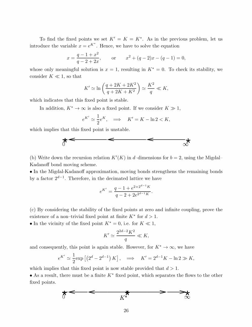
(c) By considering the stability of the fixed points at zero and infinite coupling, prove the

existence of a non–trivial fixed point at finite K∗ for d > 1.

• In the vicinity of the fixed point K∗ = 0, i.e. for K ≪ 1,

2d−2 2

K ′ 2 K≃q

≪ K,

and consequently, this point is again stable. However, for K∗ → ∞, we have

eK′ 1≃ exp 2d − 2d−1 K , = ′

2⇒ K = 2d−1K − ln 2 ≫ K,

which implies that this fix

[(

ed point is

)

now

]

stable provided that d > 1.

• As a result, there must be a finite K∗ fixed point, which separates the flows to the other

fixed points.

* * *26

(d) For d = 2, obtain K∗ and yt, for q = 3, 1, and 0.

• Let us now discuss a few particular cases in d = 2. For instance, if we consider q = 3,

the non-trivial fixed point is a solution of the equation

2 + x4x = , or x4 − 2x3 − x+ 2 = (x− 2)(x3 − 1) = 0,

1 + 2x2

which clearly yields a non-trivial fixed point at K∗ = ln 2 ≃ 0.69. The thermal exponent

for this point

∂K ′∣

∣

yt

[

e4K∗

e2K∗

6∣ = 2 = 2

∗−

∗

]

1= , = yt 0.83,

∂K K∗ e4K + 2 1 + 2e2K 9⇒ ≃

which can be compared to the exact values, K∗ = 1.005, and yt = 1.2.

By analyti

∣

c continuation for q → 1, we obtain

eK′ e4K= .−1 + 2e2K

The non-trivial fixed point is a solution of the equation

x4x = , or (x3 2

1 + 2x2− 2x2 + 1) = (x− 1)(x − x− 1) = 0,−

whose only non-trivial solution is x = (1 +√5)/2 = 1.62, resulting in K∗ = 0.48. The

thermal exponent for this point

∂K ′∣

∣ ∗

]

∣ = 2yt = 4[

1− e−K , =⇒ yt 1K K∗

≃ 0.6 .∂

As discussed in the next problem set, the Potts model for q → 1 can be mapped onto the

problem of bond percolati

∣

on, which despite being a purely geometrical phenomenon, shows

many features completely analogous to those of a continuous thermal phase transition.

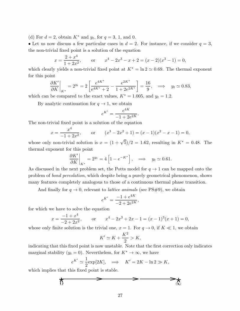
And finally for q → 0, relevant to lattice animals (see PS#9), we obtain

eK′

=−1 + e4K

,−2 + 2e2K

for which we have to solve the equation

x =−1 + x4

, or x4 − 2x3 + 2x− 1 = (x− 1)3(x+ 1) = 0,−2 + 2x2

whose only finite solution is the trivial one, x = 1. For q 0, if K 1, we obtain

K2

→ ≪

K ′ ≃ K + > K,2

indicating that this fixed point is now unstable. Note that the first correction only indicates

marginal stability (yt = 0). Nevertheless, for K∗ → ∞, we have

eK′ 1≃ exp[2K], =

2⇒ K ′ = 2K − ln 2 ≫ K,

which implies that this fixed point is stable.

* *27

********

9. The Potts model: The transfer matrix procedure can be extended to Potts model,

where the spin si on each site takes q values si = (1, 2, · · · , q); and the Hamiltonian is

−βH = K∑N

i=1 δsi,si+1+KδsN ,s1 .

(a) Write down the transfer matrix and diagonalize it. Note that you do not have to solve

a qth order secular equation as it is easy to guess the eigenvectors from the symmetry of

the matrix.

• The partition function is

Z =∑

< s1|T |s2 >< s2|T |s3 > · · · < sN−1|T |s | NN >< sN |T s1 >= tr(T ),

{si}

where < si|T |sj >= exp(

Kδsi,sj)

is a q× q transfer matrix. The diagonal elements of the

matrix are eK , while the off-diagonal elements are unity. The eigenvectors of the matrix

are easily found by inspection. There is one eigenvectors with all elements equal; the

corresponding eigenvalue is λ1 = eK +q−1. There are also (q−1) eigenvectors orthogonal

to the first, i.e. the sum of whose elements is zero. This corresponding eigenvalues are

degenerate and equal to eK − 1. Thus

Z =∑

λNα =α

(

eK + q − N1)

+ (q − 1)(

eK − 1)N

.

(b) Calculate the free energy per site.

• Since the largest eigenvalue dominates for N ≫ 1,

lnZ= ln

N

(

eK + q − 1)

.

(c) Give the expression for the correlation length ξ (you don’t need to provide a detailed

derivation), and discuss its behavior as T = 1/K → 0.

• Correlations decay as the ratio of the eigenvalues to the power of the separation. Hence

the correlation length is

[ ( )]−1 [ ( − −1λ eK1 + q 1

ξ = ln = ln .λ2 eK − 1

)]

In the limit of K → ∞, expanding the above result gives

eK 1 1ξ ≃ = exp

q q

(

T

)

.

********

28

MIT OpenCourseWarehttp://ocw.mit.edu

8.334 Statistical Mechanics II: Statistical Physics of FieldsSpring 2014

For information about citing these materials or our Terms of Use, visit: http://ocw.mit.edu/terms.