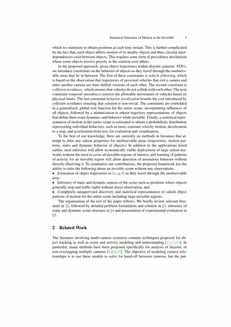
Statistical Inference of Motion in the Invisible

Haroon Idrees, Imran Saleemi, and Mubarak Shah{haroon,imran,shah}@eecs.ucf.edu

Computer Vision Lab, University of Central Florida, Orlando, USA

Abstract. This paper focuses on the unexplored problem of inferring motion ofobjects that are invisible to all cameras in a multiple camera setup. As opposed tomethods for learning relationships between disjoint cameras, we take the nextstep to actually infer the exact spatiotemporal behavior of objects while theyare invisible. Given object trajectories within disjoint cameras’ FOVs (field-of-view), we introduce constraints on the behavior of objects as they travel throughthe unobservable areas that lie in between. These constraints include vehicle fol-lowing (the trajectories of vehicles adjacent to each other at entry and exit aretime-shifted relative to each other), collision avoidance (no two trajectories passthrough the same location at the same time) and temporal smoothness (restrictsthe allowable movements of vehicles based on physical limits). The constraintsare embedded in a generalized, global cost function for the entire scene, incor-porating influences of all objects, followed by a bounded minimization using aninterior point algorithm, to obtain trajectory representations of objects that definetheir exact dynamics and behavior while invisible. Finally, a statistical represen-tation of motion in the entire scene is estimated to obtain a probabilistic distri-bution representing individual behaviors, such as turns, constant velocity motion,deceleration to a stop, and acceleration from rest for evaluation and visualization.Experiments are reported on real world videos from multiple disjoint camerasin NGSIM data set, and qualitative as well as quantitative analysis confirms thevalidity of our approach.

1 Introduction

The proliferation of large camera networks in recent past has ushered research in multi-ple camera analysis, and several methods have been proposed to address the problems ofcalibration, tracking and activity analysis with some degree of reliability [1,2,3,4,5,6,7].However, despite significant efforts in this area, the majority of literature has been con-fined to solution of problems like object correspondence and activity correlation be-tween visible objects, while estimation and inference of object behaviors in unobserv-able regions between disjoint cameras has mainly remained unexplored. Such invisibleregions between disjoint cameras are always present as visual sensor networks have aninherent inability to provide exhaustive coverage of all areas of interest, while failureof a sensor is always a possibility which can result in loss of coverage of a particulararea that was previously being observed. Besides the issue of coverage, there are sev-eral other applications that justify research into such inference: improving object cor-respondences across cameras; estimating patterns of motion and scene structure; aiding

2 Haroon Idrees, Imran Saleemi, Mubarak Shah

Fig. 1: The first image depicts the input to our method - correspondences across multipledisjoint cameras. In this case, there are five cameras, the FOV of cameras are shownwith different colors whereas invisible region is represented by black. Given the input,we reconstruct individual trajectories using constraints introduced in this paper. Next,reconstructed trajectories are used to infer expected behavior at each location in thescene, shown as thick color regions, where the direction of motion is shown by HSVcolor wheel. We also infer different behaviors such as stopping and turning from thereconstructed trajectories.

expensive operations for PTZ camera focusing by precise localization of unobservableobjects; and generalized scene understanding, etc.

In this paper, we pose the question of what information can be inferred about objectswhile they are not observable in any camera, given tracking and object correspondenceinformation in a multiple camera setup? This is an under-constrained problem, for in-stance, the correspondence provides two sets of constraints (position, velocity), but ifthe object is invisible for a hundred time steps, then we have to solve for a hundredvariables. For instance, in the scenario shown in Fig. 1, the knowledge that an objectexits a camera’s FOV on the top, and enters another’s on the right is of little use inguessing what its behavior was while invisible. The best we can do it to assume that ob-ject moved with the constant velocity through the invisible region. But, this is a ratherstrong assumption, since the object may have stopped at some unknown locations forunknown amounts of time, or may have taken an indirect path between exit and re-entryinto the camera network. Such behavior is influenced by scene structure (such as allow-able paths), obstacle avoidance, collision avoidance with other objects, and if the objectis a vehicle, it may further be influenced by dynamic aspects of the invisible scene suchas traffic signals. Besides being an assumption that is not always true, constant velocitydoes not provide with any useful information about motion of object or the invisibleregion itself. The question then becomes, can we do better than constant velocity? If weassume absolutely no information about the invisible region and treat objects indepen-dently, the answer is no. But, if we have correspondences for multiple objects available,then the fact that motion of an object is dependent on proximal objects can be used toconstrain its movement to a certain degree. The idea of using object-specific contextualconstraints has been used as social force models for tracking [8] and simulation, andfor describing vehicular motion in transportation theory [9,10,11]. But, these modelsdiffer in application from the problem addressed in his paper, in that they assume objectpositions are known with certainty, we on the other hand, use these constraints as costs

Statistical Inference of Motion in the Invisible 3

which we minimize to obtain positions at each time instant. This is further complicatedby the fact that, each object affects motion of its nearby objects and thus, circular inter-dependencies exist between objects. This requires some form of precedence mechanismwhere some objects receive priority in the solution over others.

In the proposed approach, given object trajectories within disjoint cameras’ FOVs,we introduce constraints on the behavior of objects as they travel through the unobserv-able areas that lie in between. The first of these constraints is vehicle following, whichis based on the observation that trajectories of proximal vehicles that exit a camera andenter another camera are time-shifted versions of each other. The second constraint iscollision avoidance, which ensures that vehicles do not collide with each other. The nextconstraint temporal smoothness restricts the allowable movements of vehicles based onphysical limits. The last constraint behavior localization bounds the cost introduced bycollision avoidance ensuring that solution is non-trivial. The constraints are embeddedin a generalized, global cost function for the entire scene, incorporating influences ofall objects, followed by a minimization to obtain trajectory representations of objectsthat define their exact dynamics and behavior while invisible. Finally, a statistical repre-sentation of motion in the entire scene is estimated to obtain a probabilistic distributionrepresenting individual behaviors, such as turns, constant velocity motion, decelerationto a stop, and acceleration from rest, for evaluation and visualization.

To the best of our knowledge, there are currently no methods in literature that at-tempt to infer any salient properties for unobservable areas (trajectories, motion pat-terns, static and dynamic behavior of objects). In addition to the applications listedearlier, such inference will allow economically viable deployment of large sensor net-works without the need to cover all possible regions of interest, and learning of patternsof activity for an invisible region will allow detection of anomalous behavior withoutdirectly observing it. To summarize our contributions, the proposed framework has theability to infer the following about an invisible scene without any observations:• Estimation of object trajectories in (x, y, t) as they travel through the unobservablearea,• Inference of static and dynamic aspects of the scene such as positions where objectsgenerally stop and traffic lights without direct observation, and• Completely unsupervised discovery and statistical representation of salient objectpatterns of motion for the entire scene including large invisible regions.

The organization of the rest of the paper follows. We briefly review relevant liter-ature in §2, followed by detailed problem formulation and solution in §3, inference ofstatic and dynamic scene structure in §4 and presentation of experimental evaluation in§5.

2 Related Work

The literature involving multi-camera scenarios contains techniques proposed for ob-ject tracking as well as scene and activity modeling and understanding [12,13,14]. Inparticular, many methods have been proposed specifically for analysis of disjoint, ornon-overlapping multiple cameras [4,6,5,15]. The objective of modeling camera rela-tionships is to use these models to solve for hand-off between cameras, but the pat-

4 Haroon Idrees, Imran Saleemi, Mubarak Shah

terns are modeled only for motion within the field of views of cameras. Dockstaderand Tekalp [16] use Bayesian networks for tracking and occlusion reasoning acrosscalibrated overlapping cameras while in a series of papers [17,18,19], authors employKalman Consensus Filter for tracking in multiple camera networks.

In terms of inference of topological relationships between multiple disjoint cameras,Makris et al. [3] determined the topology of a camera network by linking entry and exitzones using co-occurrence relationships between them, while Tieu et al. [20] avoid ex-plicit feature matching by computing the statistical dependence between observations indifferent cameras to infer network topology. Stauffer [21] proposed an improved linkingmethod to handle cases where exit-entry events may be correlated, but the correlationis not due to valid object transitions. Another interesting area of research is the focus ofwork by Loy et al. [7], where instead of assuming feature correspondences across cam-eras, or availability of any tracking data, regions of locally homogenous motion are firstdiscovered in all camera views using correlation of object dynamics. A canonical crosscorrelation analysis is then performed to discover and quantify the time delayed corre-lations of regional activities observed within and across multiple cameras in a commonreference space.

For our purpose of behavior inference in unobservable regions, avoidance of objectcollision in structured scenes is one of the most important cues. In this respect, researchin transportation theory has attempted to perform collision prediction and detection inthe visual domain. Atev et al. [22] propose a collision prediction algorithm using objecttrajectories, and van den Berg et al. [23] solve the problem of collision avoidance forindependently moving robots that can observe each other. In our proposed framework,however, it is essentially assumed that no collisions took place in the unobservableregion, and the goal is to infer unobserved object behavior given this assumption. Noticethat although some of the proposed constraints bear similarity to ‘motion planning’algorithms in robotics [24], some of the significant differences include the fact that forpath planning the obstacles are directly observable and the length of time taken to reachthe destination is unconstrained. Our method essentially deals with the reverse problemof path planning, i.e., inferring the path that has already been traversed. We thereforepropose a solution to a previously unexplored problem. In the following, we formallydefine the problem and discuss our approach to solve it.

3 Problem Formulation and Solution

Given a set of trajectories (for only observable areas) that have been transformed to aglobal frame-of-reference, we focus on the difficult and interesting scenario when theunobservable region contains traffic intersections even though the solution we proposein this paper can handle simpler situations such as straight roads as well. The inputvariables of the problem are the correspondences, i.e., a vehicle’s position, velocity,and time when it enters and exits the invisible region (or equivalently exits a camera’sfield of view and enters another’s).

Let pti, vti , and ati denote the position, velocity and acceleration respectively, of the

ith vehicle at time t while traveling through the invisible region and ηi and χi be thetime instants it enters and exits the invisible region. Thus, given the pair of triplets for

Statistical Inference of Motion in the Invisible 5

(a)x

y

t t t tx xx

y yy

(d)(c)(b)

Fig. 2: Depiction of constraints using vehicle trajectories in (x, y, t): (a) The point ofcollision between green and black trajectories shown with a red sphere, whereas col-lision is avoided in (b). (c) shows an example of vehicle-following behavior wherevehicle in yellow trajectory follows the one in red. In (d) the orange trajectory does notviolate smoothness constraint but the one in black does (abrupt deceleration).

entry (pη, vη, η) and exit (pχ, vχ, χ), our goal is to find pti for all t ∈ [ηi, χi], for eachvehicle which correspondingly determines vti and ati.

A path Pi is a set of 2d locations traversed by a vehicle i and is obtained by con-necting pη with pχ such that derivative of Pi is computable at all points i.e. there areno sudden turns or bends. The path so obtained does not contain any information abouttime. Associating each location in Pi with time gives us the trajectory {pti}. Two vehi-cles i and j have the same path i.e., Pi ≡ Pj , if ‖pηii − p

ηjj ‖ and ‖pχi

i − pχj

j ‖ are lessthan threshold T , and they have temporal overlap O(i, j) = 1, if ηi < χj ∧ ηj < χi.Moreover, their paths intersect, i.e., i ⊥ j, ifPi obtained by joining pηii to pχi

i , intersectswith Pj .

Since inference of motion in invisible regions in a severely under-constrained prob-lem, we impose some priors over the motion of vehicles as they travel through theregion. These priors in §3.1-3.4 below, are used as constraints that will later allow us toreconstruct complete trajectories in the invisible region. The first two constraints (col-lision avoidance and vehicle following) essentially capture the context of spatially andtemporally proximal vehicles while third constraint (smoothness of trajectories) estab-lishes physical limits on the mobility of vehicles as they travel through the region. Usingthese constraints, we propose an algorithm to reconstruct trajectories in §3.6.

3.1 Collision Avoidance

The first prior we exploit is the fact that vehicles are driven by intelligent drivers whotend to avoid collisions with each other. The probability that a vehicle will occupy alocation at particular time becomes low if the same location is occupied by anothervehicle at that same time. This effectively reduces the possible space of the solution,leaving only those solutions that have low probability of collisions. Consider the twovehicle trajectories shown in Fig. 2(a) where black trajectory shows a vehicle makinga left-turn while vehicle with green trajectory moves straight. The corresponding 2dpaths, P intersect at the point marked with a red sphere. A collision implies that asingle point in (x, y, t) is occupied by more than one object. Collision avoidance, thus,enforces that no two trajectories pass though the same (x, y, t) point. In Fig. 2(b), thecollision is avoided by a change in shape of the green trajectory. Note that, collision

6 Haroon Idrees, Imran Saleemi, Mubarak Shah

avoidance doesn’t necessarily mean that vehicles change paths in space, but that theydon’t occupy the same spatial location at the same time. Formally, let τ be the time whenvehicles with intersecting paths are closest to each other in (x, y, t), then the collisioncost for vehicle i given by:

Cαi =∑j

exp

(ωα ·

vτi .vτj

‖pτi − pτj ‖

), where τ = argmin

t

∥∥pti − ptj∥∥, (1)

∀j|i ⊥ j ∧ O(i, j) = 1, ωα being the weight. The above equation captures the costdue to motion at the point of closest approach from all vehicles with respect to the ve-hicle under consideration. The exponentiation softens the impact of collision to nearbypoints in (x, y, t), thus forcing vehicles to not only avoid the same point but avoid closeproximity as well. Two proximal vehicles both moving with a high velocity will have ahigh cost, however, if at least one vehicle is stationary, this cost will be low.

3.2 Vehicle Following

Like collision avoidance, this constraint reduces the solution space by making sure thatrelative positions of adjacent and nearby vehicles remain consistent throughout theirtravel in the invisible region. It is inspired from transportation theory, where vehiclefollowing models describe the relationship between vehicles as they move on the road-way [9,10,11]. Many of them are sophisticated functions of distance, relative velocityand acceleration of vehicles and have several parameters such as desired velocity basedon speed limit, desired spacing between vehicles and comfortable braking distance.

We, on the other hand, use vehicle following to define a spatial constraint betweenleading and following vehicles. The leader l and follower f are given by the pair:

(l, f) ={(i, j)|Pi = Pj ,O(i, j) = 1 ∧ ηi < ηj ,

χi < χj ∧ @k|ηi < ηk < ηj ∨ χi < χk < χj}. (2)

We use the relationship between leader and follower to constrain the possible move-ment of follower by forcing it to remain behind its leader throughout its travel throughthe invisible region. This also caters for the correct stopping position of follower sinceit must stop behind the leader and not occupy the same spot, an event which is highlylikely if we only take into account cost from collision. The vehicle-following cost forfollower given the leader is written as:

Cβi = exp

(ωβ∑t

‖ptj − pti‖+

), (3)

where ‖ptj − pti‖+ = ‖ptj − pti‖, if ‖ptj − pχj

j ‖ < ‖pti − pχj

j ‖ and 0 otherwise; ωβ is theweight associated to this cost.

Vehicle-following constraint enforces the condition that trajectories of vehicles ad-jacent to each other following the same path are time-shifted versions of each other,as can be seen in Fig. 2(c) where red and yellow trajectories belong to the leading andfollowing vehicles respectively.

Statistical Inference of Motion in the Invisible 7

3.3 Smoothness Of Trajectory

The smoothness constraint restricts the allowable movements of vehicles based on phys-ical limits as it happens in real life. It prevents the solution from having abrupt acceler-ation or deceleration as well as sudden stops. This is an object-centric constraint and iscomputed as:

Cγi = exp

(ωγ∑t

(1−

√π

2N (

vtivt−1i

; 1, σγ)

)), (4)

where ωγ is the weight, and N is the normal distribution with σγ = 0.25 variance.The above equation ensures that distance in space-time volume between any two

adjacent points in a single trajectory is a small multiple of the other. In Fig. 2(d), theorange trajectory is has low smoothness cost whereas black trajectory has higher costdue to abrupt deceleration in the beginning.

3.4 Stopping Behavior Localization

The above three constraints do not completely specify the solution because trivial solu-tions with high values of acceleration and deceleration can exist. This is possible whena vehicle is made to stop with high deceleration i.e. near pηii , stays there as long aspossible before leaving the invisible region with high acceleration while satisfying thesmoothness constraint. This afraid-of-collision solution for a vehicle is not only incor-rect, it also will result in wrong results for all of the following vehicles. The followingadditional cost will rectify this problem avoiding such solution,

Cδi = exp(ωδ∥∥∥xi,j − ptϕi ∥∥∥) , j|i⊥j ∧ O(i, j) = 1, (5)

where ωδ is the associated weight, xi,j is the spatial point where vehicle paths intersectand tϕ is the time when vehicle stops. This constraint dictates that stopping point fora vehicle cannot be arbitrarily away from the possible collision locations, essentiallylocalizing the move-stop-move events in space and time.

3.5 Trajectory Parametrization

As mentioned earlier, given entry and exit locations, each trajectory is represented by a2D path, P by joining the two locations in a way that allows for bends as they happenin the case of turns. Parameterizing the curve by placing χ− η equidistant points for avehicle gives us a trajectory that represents motion with constant velocity. Parameteriz-ing in this way reduces the number of variables to one-half (from 2D to 1D). Our goalthen becomes to find the temporal parametrization of the trajectory that minimizes costfrom the constraints. But, given that we might be dealing with thousands of vehicles,each invisible for hundreds of time units, the extremely large variable space (∼ 106)makes the problem intractable.

In order to make the problem tractable, we reduce the parameters defining a trajec-tory to three: deceleration (φ), duration of stopping time (ϕ) and acceleration (ψ). The

8 Haroon Idrees, Imran Saleemi, Mubarak Shah

321t=81 381 521 681

t=1101 14611301 16411361

Fig. 3: Each row is an example of trajectory reconstruction. Vehicle under considerationis shown with squares, yellow depicts constant velocity, red is from proposed methodand green square marks the ground truth. Rest of the vehicles are shown in black. In firstrow, reconstruction with constant velocity causes collisions at t = 381 and 521, and inthe second row, between t = 1200 and 1500. On the other hand, proposed method andground truth allow the vehicles to pass without any collision.

constant velocity case corresponds to φ = ϕ = ψ = 0. Thus, we can model all casesbetween constant velocity to complete stopping by varying values of these variables.However, since the exact duration of invisibility and end-point velocities are known,we have only two-degrees of freedom making one of the variables dependent on theother two. We choose φ and ϕ to represent the trajectory, while ψ is determined basedon time and velocity constraints. Thus, the parametrization results in constant or zeroacceleration and deceleration while satisfying entry and exit velocities.

3.6 Optimization for Motion Inference

Considering each vehicle individually, given the time it enters and exits the region, thebest estimate for its motion is constant velocity. However, since an invisible region (inour case, an intersection) may involve vehicles traveling in from all directions, eachvehicle influences the motion of other vehicles. A constant velocity prediction for eachvehicle will result in collisions even though it may satisfy the constraints of vehicle-following and smoothness.

Given entry and exit triplets of position, velocity and time for each vehicle, our goalis to find the parameters φ and ϕ for all vehicles that pass though the invisible region.Since each vehicle’s position at every time instant is conditionally dependent on allother vehicles that also pass through the invisible region, this information is exploitedin the form of four constraints. The proposed solution iteratively minimizes the localcost of each vehicle by making sure it satisfies the constraints, fixing its parameters andthen moving onto other vehicles.

Statistical Inference of Motion in the Invisible 9

Algorithm 1 Algorithm to infer motion of vehicles given [pη, vη, η] and [pχ, vχ, χ] forvehicles 1 : n1: procedure INVISIBLEINFERENCE

2: Prioritize vehicles using Eq. 63: for all i← 1, n as per Θi do4: Identify j|O(i, j) = 1 and i⊥j5: φi, ϕi ← argmin

φ,ϕCαi + Cβi + Cγi + Cδi

6: Parameterize trajectory i according to φi, ϕi7: end for8: end procedure

We impose a prioritizing function on the trajectories, which is a linear function ofentry and exit times:

Θi = ωχχi + ωηηi. (6)

If we set ωχ = 1 and ωη = −1, the criteria becomes shortest duration first, on theother hand, if ωχ = 1 and ωη = 0, the criteria becomes earlier exit first. The formerbiases the solution towards high priority vehicles putting very strong constraints onvehicles that spend longer times in the invisible region. We used the latter which makesmore intuitive sense also since vehicles will yield way to the a vehicle that exits beforethem.

The cost for each vehicle is the sum of costs due to collision, vehicle-following, andsmoothness including penalty for trivial solution. The parameters are bounded so that−20 ft/s2 < φ < 0, and 0 < ϕ < χ− η, and the cost is minimized through an InteriorPoint Algorithm with initialization provided by uniform grid search over the parameterspace. The summary for this simple algorithm is provided in Alg. 1 while Fig. 3 showsthe results on real examples.

4 Inference of Scene Structure

After obtaining trajectories using the method and constraints described in the previoussection, we now propose methods to statistically represent motion in the invisible re-gion (§4.1), followed by extracting some key features of the scene such as locations ofstopping points (static) and timings of traffic signals (dynamic) in §4.2.

4.1 Statistical Representation of Motion

Given the inferred trajectory representations for objects in invisible region, we computethe features, (xti, y

ti , u

ti, v

ti , t), for each point on the ith trajectory derived from Pi, φi,

ϕi, and ψi, where ut = xt − xt−1, and vt = yt − yt−1. To obtain a probabilisticdistribution that represent individual behaviors, such as turns, constant velocity motion,deceleration to a stop, and acceleration from rest, we first cluster feature points using the

10 Haroon Idrees, Imran Saleemi, Mubarak Shah

k-means algorithm, and then treat the clusters as components of a 4d Gaussian mixturemodel, B for each leg of traffic. A feature point x induced by B is given as,

x ∼NB∑k=1

ωkN(·∣∣∣µk,Σk

), (7)

where the mixture contains NB Gaussian components, each with parameters µ, Σ, andmixing proportion ω. This representation serves as a generative model that summarizesthe spatiotemporal dynamics of objects induced by each behavior, and is potentiallyuseful for scene understanding, anomaly detection, tracking and data association, aswell as visualization of results of the proposed inference framework. For visualization,we compute the per-pixel expected motion vectors conditioned on the pixel locationalong each leg, i.e., EB

[√u2 + v2, tan−1(v/u)|x, y

], to obtain expected magnitude

and orientation of motion at each pixel for each behavior, and depict them using theHSV colormap as is done for motion patterns [25].

4.2 Scene Structure & Status Inference

Given the exact motion and behavior of objects in the invisible regions, we propose toestimate some key aspects of the scene structure and status to, show the importanceand usefulness of our framework, and allow evaluation. We briefly explain our methodsfor finding the locations where vehicles exhibit the stopping behavior (equivalent tostopping positions), and the times at which such behaviors occur (equivalent to statusof traffic signals) for each path in the invisible region.

We use the locations, ptϕi , for i|vi < T , to vote for regions corresponding to stoppositions. Specifically, given n vehicles, we compute the following kernel density esti-mate of the 2d surface, Γ , representing probability of a pixel, p, belonging to stoppinglocation:

Γ (p) =1

n|H|− 1

2

n∑i=1

K(

H− 12

(p− ptϕi

)), (8)

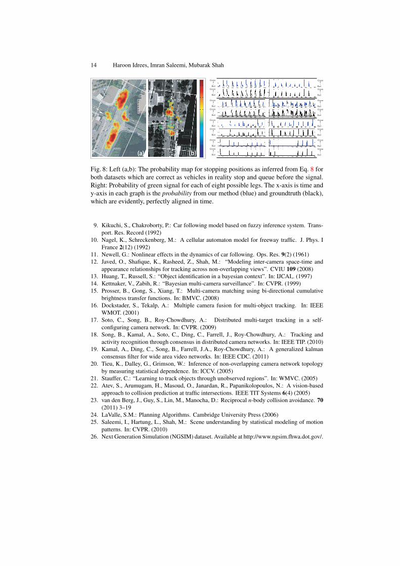
where K is a 2d Gaussian kernel with a symmetric, positive, diagonal bandwidth ma-trix, H, of fixed horizontal and vertical variances, set to 10 pixels. Fig. 8(a,b) shows anexample of the distribution reflecting probabilities of pixels being stopping positions.The proposed framework therefore estimates salient scene structure in a statistical man-ner, without making a single observation within the scene.

Secondly, given the representation of behaviors learned earlier which divides thescene into possibly overlapping segments corresponding to traffic intersection legs, bythresholding

∫ ∫PrBdudv, we can effectively estimate the signal status for each leg.

We use the following simple process: at a given time t, the inferred status (red, green)of a traffic signal for a leg, l, is

∑i ‖p

t+1i − pti‖, if i belongs to l and t > tϕ. Therefore,

if any vehicle traveling on leg l has a non-negligible velocity at its stopping positions,it votes for the green signal for that leg at that time. The results of signal status andtransitions for all legs of traffic (blue), compared to the results obtained by applying thesame process to ground truth trajectories (black), are shown in Fig.8(c).

Statistical Inference of Motion in the Invisible 11

xx

yy

t

t

Fig. 4: All trajectories inferred for each dataset shown in 3D. Left and right images areinferred trajectories from Lankershim and Peachtree datasets respectively.

(a) (b) (c) (d)

Fig. 5: Trajectories in (a) and (c) represent constant velocity while (b) and (d) showoutput of proposed method. Collisions due to constant velocity prediction are markedwith red spheres in (a) and (c), but this does not occur in (b) and (d), which are theresults of proposed trajectory inference.

5 Experiments

We ran our experiments on two datasets from NGSIM (see [26] for details). The firstinvisible region was from Lankershim 8:30am - 8:45am located at the intersectionof Lankershim/Universal Hollywood Dr. (LA) with a total of 1211 vehicles passingthrough the region. The second invisible region was from Peachtree 4:00pm to 4:15pmlocated at the intersection of Peachtree/10th Street NE (Atlanta) with 657 vehicles pass-ing through the region. Both intersections were typical four-legged with three possiblepaths that could be taken by a vehicle entering a particular leg, thus, resulting in 12 totalpaths. Fig. 4 shows the trajectories that were output by Alg. 1 for both the datasets.

We next analyze the performance of motion inference employing the different con-straints, followed by results for motion behaviors and scene structure. Figure 5 providesqualitative results for motion inference where the (a,b) is from Peachtree and (c,d) fromLankershim dataset. The black trajectory corresponds to the vehicle under considera-tion while proximal vehicles which it could possibly collide with are shown in colors.In both (a) and (c), the trajectories are drawn assuming constant velocity for each ve-hicle. In (a), the vehicle collides with one of the vehicles whereas in (c), vehicle underconsideration collides with six different vehicles. The locations of collision are shownwith red spheres partially invisible due to other vehicles. Notice the change in shape in

12 Haroon Idrees, Imran Saleemi, Mubarak Shah

Tota

l Err

or /

Tra

ject

ory

Vehicle ID Distance (feet)

Perc

enta

ge

Co

rrec

t

(a) (b) (c)

Fig. 6: (a,b) Error profile for our method (yellow) vs. constant velocity (black) for bothdatasets. As can be seen, our method has lower error (it has smaller magnitude), thusprovides more accurate inference. (c) ROC curves for our method (solid) vs. constantvelocity (dashed) for the Lankershim (red) and Peachtree (green). The x-axis is thedistance threshold in feet while y-axis gives the percentage of points that lie within thatthreshold distance of the ground-truth.

(b) and (d) after inferring motion for all trajectories with the outcome that none of thetrajectories collides with the black trajectory. Both vehicle-following and smoothnessconstraints are also visibly in effect in both the examples.

Fig. 6(a,b) gives a per-trajectory comparison of error with and without motion infer-ence. These graphs for Lankershim and Peachtree respectively were obtained by com-puting total error (in feet) for each trajectory by computing Euclidean distance of eachpoint to the groundtruth. The yellow bars correspond to motion inference whereas blackbars represent the case of using constant velocity only. Fig. 6(c) gives the ROC curvesfor the two datasets. On the x-axis is the threshold distance in feet, on y-axis are thepercentage of points in all invisible trajectories that lie within that threshold. Using in-ference, we get an improvement of at least 20% over the baseline in both datasets. Afterobtaining the inferred trajectories, we statistically represented the motion in the invisi-ble region using the method described in §4.1. Fig. 7 shows MoG for three different legswhere three columns represent constant velocity, proposed method and ground truth.

Figures 8 give results for some of the salient features of the invisible region using§4.2. Fig. 8(a) shows the probability map superimposed on the image of invisible regionfor locations where vehicles stop using only the inferred trajectories from Lankershimwhereas Fig. 8(b) shows the same probability map for Peachtree. It can be seen thatall of the locations are correct, just before the intersection due to collision avoidanceand extend beyond due to vehicle following constraint when vehicles queue up at in-tersection. Figure 8(c) gives the probability of which traffic light was green at eachtime instant using the proposed method (blue) and the results are also compared againstgroundtruth (black). In this figure, we show traffic light behavior over time for 8 of the12 paths as right turns do not get subjected to signals. Below each blue graph whichis obtained using inferred trajectories, is the black graph showing probability of thatlight being green using groundtruth. The results show little difference, validating theperformance and quality of inference.

Statistical Inference of Motion in the Invisible 13

Constant Velocity Proposed Method Ground Truth

Fig. 7: Each row is the Mixture of Gaussians representation for a particular path usingconstant velocity, proposed method and ground truth. The patterns in the second andthird column are similar and capture acceleration, deceleration, start and stop behaviorswhereas in first column, all Gaussians have the same variance due to constant velocity.

6 Conclusion and Future Work

We presented the novel idea of understanding motion behavior of objects while theyare in the invisible region of multiple proximal cameras. The solution used three con-straints, two of which employ contextual information of neighboring objects to infercorrect motion of object under consideration. Though, an interesting proposal from theperspective of scene and motion understanding, the idea has several potential applica-tions in video surveillance. Possible extensions include handling situations where cor-respondences are missing or incorrect in some cases and to humans where social forcemodels can be leveraged in addition to current constraints.

References

1. Stauffer, C., Tieu, K.: Automated multi-camera planar tracking correspondence modeling.In: CVPR. (2003)

2. Khan, S., Shah, M.: Consistent labeling of tracked objects in multiple cameras with overlap-ping fields of view. IEEE PAMI 25 (2003)

3. Makris, D., Ellis, T., Black, J.: Bridging the gaps between cameras. In: CVPR. (2004)4. Gheissari, N., Sebastian, T., Hartley, R.: Person reidentification using spatiotemporal appear-

ance. In: CVPR. Volume 2. (2006)5. Hu, W., Hu, M., Zhou, X., Tan, T., Lou, J., Maybank, S.: Principal axis-based correspondence

between multiple cameras for people tracking. IEEE PAMI 28(4) (2006)6. Gray, D., Tao, H.: Viewpoint invariant pedestrian recognition with an ensemble of localized

features. In: ECCV. (2008)7. Loy, C.C., Xiang, T., Gong, S.: Multi-camera activity correlation analysis. In: CVPR. (2009)8. Pellegrini, S., Ess, A., Schindler, K., van Gool, L.: You’ll never walk alone: Modeling social

behavior for multi-target tracking. In: ICCV. (2009)

14 Haroon Idrees, Imran Saleemi, Mubarak Shah

Red

Green

Red

GreenRed

Green

Red

Green

Red

Green

Red

Green

Red

Green

Red

Green

Red

Green

Red

GreenRed

Green

Red

Green

Red

Green

Red

Green

Red

Green

Red

Green

(a)(a) (b)(b)

Fig. 8: Left (a,b): The probability map for stopping positions as inferred from Eq. 8 forboth datasets which are correct as vehicles in reality stop and queue before the signal.Right: Probability of green signal for each of eight possible legs. The x-axis is time andy-axis in each graph is the probability from our method (blue) and groundtruth (black),which are evidently, perfectly aligned in time.

9. Kikuchi, S., Chakroborty, P.: Car following model based on fuzzy inference system. Trans-port. Res. Record (1992)

10. Nagel, K., Schreckenberg, M.: A cellular automaton model for freeway traffic. J. Phys. IFrance 2(12) (1992)

11. Newell, G.: Nonlinear effects in the dynamics of car following. Ops. Res. 9(2) (1961)12. Javed, O., Shafique, K., Rasheed, Z., Shah, M.: “Modeling inter-camera space-time and

appearance relationships for tracking across non-overlapping views”. CVIU 109 (2008)13. Huang, T., Russell, S.: “Object identification in a bayesian context”. In: IJCAI,. (1997)14. Kettnaker, V., Zabih, R.: “Bayesian multi-camera surveillance”. In: CVPR. (1999)15. Prosser, B., Gong, S., Xiang, T.: Multi-camera matching using bi-directional cumulative

brightness transfer functions. In: BMVC. (2008)16. Dockstader, S., Tekalp, A.: Multiple camera fusion for multi-object tracking. In: IEEE

WMOT. (2001)17. Soto, C., Song, B., Roy-Chowdhury, A.: Distributed multi-target tracking in a self-

configuring camera network. In: CVPR. (2009)18. Song, B., Kamal, A., Soto, C., Ding, C., Farrell, J., Roy-Chowdhury, A.: Tracking and

activity recognition through consensus in distributed camera networks. In: IEEE TIP. (2010)19. Kamal, A., Ding, C., Song, B., Farrell, J.A., Roy-Chowdhury, A.: A generalized kalman

consensus filter for wide area video networks. In: IEEE CDC. (2011)20. Tieu, K., Dalley, G., Grimson, W.: Inference of non-overlapping camera network topology

by measuring statistical dependence. In: ICCV. (2005)21. Stauffer, C.: “Learning to track objects through unobserved regions”. In: WMVC. (2005)22. Atev, S., Arumugam, H., Masoud, O., Janardan, R., Papanikolopoulos, N.: A vision-based

approach to collision prediction at traffic intersections. IEEE TIT Systems 6(4) (2005)23. van den Berg, J., Guy, S., Lin, M., Manocha, D.: Reciprocal n-body collision avoidance. 70

(2011) 3–1924. LaValle, S.M.: Planning Algorithms. Cambridge University Press (2006)25. Saleemi, I., Hartung, L., Shah, M.: Scene understanding by statistical modeling of motion

patterns. In: CVPR. (2010)26. Next Generation Simulation (NGSIM) dataset. Available at http://www.ngsim.fhwa.dot.gov/.