
Statistical Distributions, 4th ed. - Istituto Nazionale di...
231
Transcript of Statistical Distributions, 4th ed. - Istituto Nazionale di...


Statistical Distributions

Statistical DistributionsFourth Edition
Catherine ForbesMonash University, Victoria, Australia
Merran EvansMonash University, Victoria, Australia
Nicholas HastingsAlbany Interactive, Victoria, Australia
Brian PeacockBrian Peacock Ergonomics, SIM University, Singapore

Copyright © 2011 by John Wiley & Sons, Inc. All rights reserved.
Published by John Wiley & Sons, Inc., Hoboken, New Jersey.Published simultaneously in Canada.
No part of this publication may be reproduced, stored in a retrieval system, or transmitted in any form orby any means, electronic, mechanical, photocopying, recording, scanning, or otherwise, except aspermitted under Section 107 or 108 of the 1976 United States Copyright Act, without either the priorwritten permission of the Publisher, or authorization through payment of the appropriate per-copy fee tothe Copyright Clearance Center, Inc., 222 Rosewood Drive, Danvers, MA 01923, (978) 750-8400, fax(978) 750-4470, or on the web at www.copyright.com. Requests to the Publisher for permission shouldbe addressed to the Permissions Department, John Wiley & Sons, Inc., 111 River Street, Hoboken, NJ07030, (201) 748-6011, fax (201) 748-6008, or online at http://www.wiley.com/go/permission.
Limit of Liability/Disclaimer of Warranty: While the publisher and author have used their best efforts inpreparing this book, they make no representations or warranties with respect to the accuracy orcompleteness of the contents of this book and specifically disclaim any implied warranties ofmerchantability or fitness for a particular purpose. No warranty may be created or extended by salesrepresentatives or written sales materials. The advice and strategies contained herein may not be suitablefor your situation. You should consult with a professional where appropriate. Neither the publisher norauthor shall be liable for any loss of profit or any other commercial damages, including but not limited tospecial, incidental, consequential, or other damages.
For general information on our other products and services or for technical support, please contact ourCustomer Care Department within the United States at (800) 762-2974, outside the United States at (317)572-3993 or fax (317) 572-4002.
Wiley also publishes its books in a variety of electronic formats. Some content that appears in print maynot be available in electronic formats. For more information about Wiley products, visit our web site atwww.wiley.com.
Library of Congress Cataloging-in-Publication Data:
Statistical distributions. – 4th ed. / Catherine Forbes . . . [et al.].p. cm. – (Wiley series in probability and statistics)
Includes bibliographical references and index.ISBN 978-0-470-39063-4 (pbk.)
1. Distribution (Probability theory) I. Forbes, Catherine.QA273.6.E92 2010519.2’4–dc22
2009052131
Printed in the United States of America.
10 9 8 7 6 5 4 3 2 1


TOJeremy and Elana ForbesCaitlin and Eamon Evans
Tina HastingsEileen Peacock

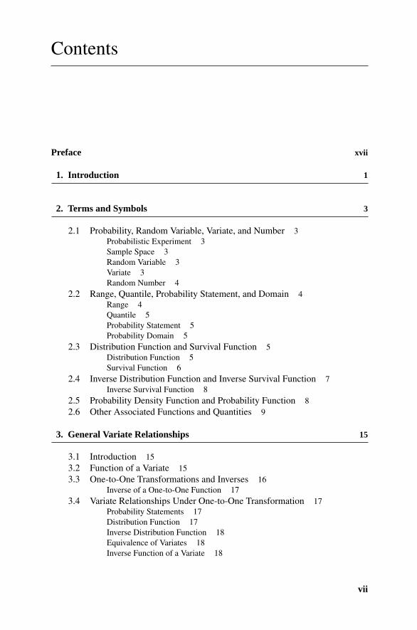
Contents
Preface xvii
1. Introduction 1
2. Terms and Symbols 3
2.1 Probability, Random Variable, Variate, and Number 3Probabilistic Experiment 3Sample Space 3Random Variable 3Variate 3Random Number 4
2.2 Range, Quantile, Probability Statement, and Domain 4Range 4Quantile 5Probability Statement 5Probability Domain 5
2.3 Distribution Function and Survival Function 5Distribution Function 5Survival Function 6
2.4 Inverse Distribution Function and Inverse Survival Function 7Inverse Survival Function 8
2.5 Probability Density Function and Probability Function 82.6 Other Associated Functions and Quantities 9
3. General Variate Relationships 15
3.1 Introduction 153.2 Function of a Variate 153.3 One-to-One Transformations and Inverses 16
Inverse of a One-to-One Function 173.4 Variate Relationships Under One-to-One Transformation 17
Probability Statements 17Distribution Function 17Inverse Distribution Function 18Equivalence of Variates 18Inverse Function of a Variate 18
vii

viii Contents
3.5 Parameters, Variate, and Function Notation 19Variate and Function Notation 19
3.6 Transformation of Location and Scale 203.7 Transformation from the Rectangular Variate 203.8 Many-to-One Transformations 22
Symmetrical Distributions 22
4. Multivariate Distributions 24
4.1 Joint Distributions 24Joint Range 24Bivariate Quantile 24Joint Probability Statement 24Joint Probability Domain 25Joint Distribution Function 25Joint Probability Density Function 25Joint Probability Function 25
4.2 Marginal Distributions 26Marginal Probability Density Function and MarginalProbability Function 26
4.3 Independence 274.4 Conditional Distributions 28
Conditional Probability Function and ConditionalProbability Density Function 28Composition 29
4.5 Bayes’ Theorem 304.6 Functions of a Multivariate 30
5. Stochastic Modeling 32
5.1 Introduction 325.2 Independent Variates 325.3 Mixture Distributions 33
Finite Mixture 33Infinite Mixture of Distributions 35
5.4 Skew-Symmetric Distributions 385.5 Distributions Characterized by Conditional Skewness 395.6 Dependent Variates 42
6. Parameter Inference 44
6.1 Introduction 446.2 Method of Percentiles Estimation 446.3 Method of Moments Estimation 456.4 Maximum Likelihood Inference 47
Properties of MLEs 47Approximate Sampling Distribution for Fixed n 48

Contents ix
6.5 Bayesian Inference 50Marginal Posteriors 51
7. Bernoulli Distribution 53
7.1 Random Number Generation 537.2 Curtailed Bernoulli Trial Sequences 537.3 Urn Sampling Scheme 547.4 Note 54
8. Beta Distribution 55
8.1 Notes on Beta and Gamma Functions 56Definitions 56Interrelationships 56Special Values 57Alternative Expressions 57
8.2 Variate Relationships 578.3 Parameter Estimation 598.4 Random Number Generation 608.5 Inverted Beta Distribution 608.6 Noncentral Beta Distribution 618.7 Beta Binomial Distribution 61
9. Binomial Distribution 62
9.1 Variate Relationships 649.2 Parameter Estimation 659.3 Random Number Generation 65
10. Cauchy Distribution 66
10.1 Note 6610.2 Variate Relationships 6710.3 Random Number Generation 6810.4 Generalized Form 68
11. Chi-Squared Distribution 69
11.1 Variate Relationships 7111.2 Random Number Generation 7211.3 Chi Distribution 73
12. Chi-Squared (Noncentral) Distribution 74
12.1 Variate Relationships 75

x Contents
13. Dirichlet Distribution 77
13.1 Variate Relationships 7713.2 Dirichlet Multinomial Distribution 78
14. Empirical Distribution Function 79
14.1 Estimation from Uncensored Data 7914.2 Estimation from Censored Data 7914.3 Parameter Estimation 8114.4 Example 8114.5 Graphical Method for the Modified Order-Numbers 8114.6 Model Accuracy 83
15. Erlang Distribution 84
15.1 Variate Relationships 8515.2 Parameter Estimation 8515.3 Random Number Generation 85
16. Error Distribution 86
16.1 Note 8716.2 Variate Relationships 87
17. Exponential Distribution 88
17.1 Note 8917.2 Variate Relationships 9117.3 Parameter Estimation 9217.4 Random Number Generation 92
18. Exponential Family 93
18.1 Members of the Exponential Family 9318.2 Univariate One-Parameter Exponential Family 9318.3 Parameter Estimation 9518.4 Generalized Exponential Distributions 95
Generalized Student’s t Distribution 95Variate Relationships 96Generalized Exponential Normal Distribution 96Generalized Lognormal Distribution 96Variate Relationships 97

Contents xi
19. Extreme Value (Gumbel) Distribution 98
19.1 Note 9919.2 Variate Relationships 10019.3 Parameter Estimation 10119.4 Random Number Generation 101
20. F (Variance Ratio) or Fisher–Snedecor Distribution 102
20.1 Variate Relationships 103
21. F (Noncentral) Distribution 107
21.1 Variate Relationships 108
22. Gamma Distribution 109
22.1 Variate Relationships 11022.2 Parameter Estimation 11122.3 Random Number Generation 11222.4 Inverted Gamma Distribution 11222.5 Normal Gamma Distribution 11222.6 Generalized Gamma Distribution 113
Variate Relationships 113
23. Geometric Distribution 114
23.1 Notes 11523.2 Variate Relationships 11523.3 Random Number Generation 116
24. Hypergeometric Distribution 117
24.1 Note 11824.2 Variate Relationships 11824.3 Parameter Estimation 11824.4 Random Number Generation 11924.5 Negative Hypergeometric Distribution 11924.6 Generalized Hypergeometric Distribution 119
25. Inverse Gaussian (Wald) Distribution 120
25.1 Variate Relationships 12125.2 Parameter Estimation 121
xii Contents
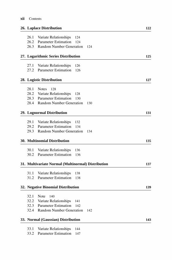
26. Laplace Distribution 122
26.1 Variate Relationships 12426.2 Parameter Estimation 12426.3 Random Number Generation 124
27. Logarithmic Series Distribution 125
27.1 Variate Relationships 12627.2 Parameter Estimation 126
28. Logistic Distribution 127
28.1 Notes 12828.2 Variate Relationships 12828.3 Parameter Estimation 13028.4 Random Number Generation 130
29. Lognormal Distribution 131
29.1 Variate Relationships 13229.2 Parameter Estimation 13429.3 Random Number Generation 134
30. Multinomial Distribution 135
30.1 Variate Relationships 13630.2 Parameter Estimation 136
31. Multivariate Normal (Multinormal) Distribution 137
31.1 Variate Relationships 13831.2 Parameter Estimation 138
32. Negative Binomial Distribution 139
32.1 Note 14032.2 Variate Relationships 14132.3 Parameter Estimation 14232.4 Random Number Generation 142
33. Normal (Gaussian) Distribution 143
33.1 Variate Relationships 14433.2 Parameter Estimation 147

Contents xiii
33.3 Random Number Generation 14733.4 Truncated Normal Distribution 14733.5 Variate Relationships 148
34. Pareto Distribution 149
34.1 Note 14934.2 Variate Relationships 15034.3 Parameter Estimation 15134.4 Random Number Generation 151
35. Poisson Distribution 152
35.1 Note 15335.2 Variate Relationships 15335.3 Parameter Estimation 15635.4 Random Number Generation 156
36. Power Function Distribution 157
36.1 Variate Relationships 15736.2 Parameter Estimation 15936.3 Random Number Generation 159
37. Power Series (Discrete) Distribution 160
37.1 Note 16037.2 Variate Relationships 16137.3 Parameter Estimation 161
38. Queuing Formulas 162
38.1 Characteristics of Queuing Systems and Kendall-Lee Notation 162Characteristics of Queuing Systems 162Kendall-Lee Notation 164
38.2 Definitions, Notation, and Terminology 164Steady State 164Traffic Intensity and Traffic Density 164Notation and Terminology 164
38.3 General Formulas 16638.4 Some Standard Queuing Systems 166
The M/M/1/G/∞/∞ System 166The M/M/s/G/ ∞/∞ System 166The M/G/1/G/∞/∞ System (Pollaczek-Khinchin) 168The M/M/1/G/m/∞ System 168The M/G/m/G/m/∞ System (Erlang) 169
xiv Contents
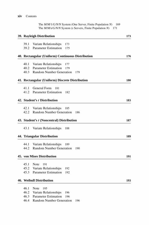
The M/M/1/G/N/N System (One Server, Finite Population N) 169The M/M/s/G/N/N System (s Servers, Finite Population N) 171
39. Rayleigh Distribution 173
39.1 Variate Relationships 17339.2 Parameter Estimation 175
40. Rectangular (Uniform) Continuous Distribution 176
40.1 Variate Relationships 17740.2 Parameter Estimation 17940.3 Random Number Generation 179
41. Rectangular (Uniform) Discrete Distribution 180
41.1 General Form 18141.2 Parameter Estimation 182
42. Student’s t Distribution 183
42.1 Variate Relationships 18542.2 Random Number Generation 186
43. Student’s t (Noncentral) Distribution 187
43.1 Variate Relationships 188
44. Triangular Distribution 189
44.1 Variate Relationships 18944.2 Random Number Generation 190
45. von Mises Distribution 191
45.1 Note 19145.2 Variate Relationships 19245.3 Parameter Estimation 192
46. Weibull Distribution 193
46.1 Note 19546.2 Variate Relationships 19646.3 Parameter Estimation 19646.4 Random Number Generation 196
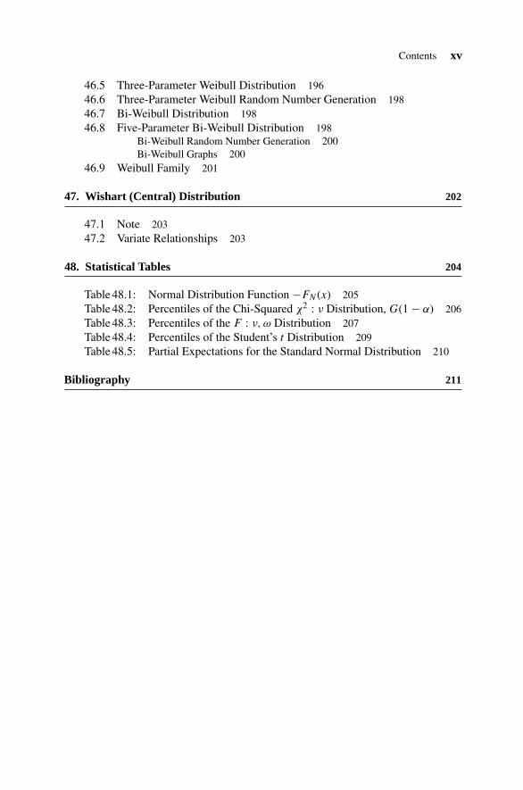
Contents xv
46.5 Three-Parameter Weibull Distribution 19646.6 Three-Parameter Weibull Random Number Generation 19846.7 Bi-Weibull Distribution 19846.8 Five-Parameter Bi-Weibull Distribution 198
Bi-Weibull Random Number Generation 200Bi-Weibull Graphs 200
46.9 Weibull Family 201
47. Wishart (Central) Distribution 202
47.1 Note 20347.2 Variate Relationships 203
48. Statistical Tables 204
Table 48.1: Normal Distribution Function −FN (x) 205Table 48.2: Percentiles of the Chi-Squared χ2 : ν Distribution, G(1 − α) 206Table 48.3: Percentiles of the F : ν, ω Distribution 207Table 48.4: Percentiles of the Student’s t Distribution 209Table 48.5: Partial Expectations for the Standard Normal Distribution 210
Bibliography 211

Preface
This revised handbook provides a concise summary of the salient facts and formu-las relating to 40 major probability distributions, together with associated diagramsthat allow the shape and other general properties of each distribution to be readilyappreciated.
In the introductory chapters the fundamental concepts of the subject are coveredwith clarity, and the rules governing the relationships between variates are described.Extensive use is made of the inverse distribution function and a definition establishesa variate as a generalized form of a random variable. A consistent and unambiguoussystem of nomenclature can thus be developed, with chapter summaries relating toindividual distributions.
Students, teachers, and practitioners for whom statistics is either a primary orsecondary discipline will find this book of great value, both for factual references andas a guide to the basic principles of the subject. It fulfills the need for rapid access toinformation that must otherwise be gleaned from many scattered sources.
The first version of this book, written by N. A. J. Hastings and J. B. Peacock, waspublished by Butterworths, London, 1975. The second edition, with a new author,M. A. Evans, was published by John Wiley & Sons in 1993, with a third editionby the same authors published by John Wiley & Sons in 2000. This fourth editionsees the addition of a new author, C. S. Forbes. Catherine Forbes holds a Ph.D.in Mathematical Statistics from The Ohio State University, USA, and is currentlySenior Lecturer at Monash University, Victoria, Australia. Professor Merran Evansis currently Pro Vice-Chancellor, Planning and Quality at Monash University andobtained her Ph.D. in Econometrics from Monash University. Dr. Nicholas Hastingsholds a Ph.D. in Operations Research from the University of Birmingham. FormerlyMount Isa Mines Professor of Maintenance Engineering at Queensland University ofTechnology, Brisbane, Australia, he is currently Director and Consultant in physicalasset management, Albany Interactive Pty Ltd. Dr. Brian Peacock has a backgroundin ergonomics and industrial engineering which have provided a foundation for along career in industry and academia, including 18 years in academia, 15 years withGeneral Motors’ vehicle design and manufacturing organizations, and 4 years asdiscipline coordinating scientist for the National Space Biomedical Institute/NASA.He is a licensed professional engineer, a licensed private pilot, a certified professionalergonomist, and a fellow of both the Ergonomics and Human Factors Society (UK) andthe Human Factors and Ergonomics Society (USA). He recently retired as a professorin the Department of Safety Science at Embry Riddle Aeronautical University, wherehe taught classes in system safety and applied ergonomics.
xvii

xviii Preface
The authors gratefully acknowledge the helpful suggestions and comments madeby Harry Bartlett, Jim Conlan, Benoit Dulong, Alan Farley, Robert Kushler, Jerry W.Lewis, Allan T. Mense, Grant Reinman, and Dimitris Ververidis.
Catherine ForbesMerran EvansNicholas HastingsBrian Peacock

Chapter 1
Introduction
The number of puppies in a litter, the life of a light bulb, and the time to arrival ofthe next bus at a stop are all examples of random variables encountered in everydaylife. Random variables have come to play an important role in nearly every field ofstudy: in physics, chemistry, and engineering, and especially in the biological, social,and management sciences. Random variables are measured and analyzed in termsof their statistical and probabilistic properties, an underlying feature of which is thedistribution function. Although the number of potential distribution models is verylarge, in practice a relatively small number have come to prominence, either becausethey have desirable mathematical characteristics or because they relate particularlywell to some slice of reality or both.
This book gives a concise statement of leading facts relating to 40 distributionsand includes diagrams so that shapes and other general properties may readily beappreciated. A consistent system of nomenclature is used throughout. We have foundourselves in need of just such a summary on frequent occasions—as students, asteachers, and as practitioners. This book has been prepared and revised in an attemptto fill the need for rapid access to information that must otherwise be gleaned fromscattered and individually costly sources.
In choosing the material, we have been guided by a utilitarian outlook. For ex-ample, some distributions that are special cases of more general families are givenextended treatment where this is felt to be justified by applications. A general dis-cussion of families or systems of distributions was considered beyond the scope ofthis book. In choosing the appropriate symbols and parameters for the description ofeach distribution, and especially where different but interrelated sets of symbols arein use in different fields, we have tried to strike a balance between the various usages,the need for a consistent system of nomenclature within the book, and typographicsimplicity. We have given some methods of parameter estimation where we felt itwas appropriate to do so. References listed in the Bibliography are not the primarysources but should be regarded as the first “port of call”.
In addition to listing the properties of individual variates we have consideredrelationships between variates. This area is often obscure to the nonspecialist. We
Statistical Distributions, Fourth Edition, by Catherine Forbes, Merran Evans, Nicholas Hastings,and Brian PeacockCopyright © 2011 John Wiley & Sons, Inc.
1

2 Chapter 1 Introduction
have also made use of the inverse distribution function, a function that is widelytabulated and used but rarely explicitly defined. We have particularly sought to avoidthe confusion that can result from using a single symbol to mean here a function,there a quantile, and elsewhere a variate.
Building on the three previous editions, this fourth edition documents recentextensions to many of these probability distributions, facilitating their use in morevaried applications. Details regarding the connection between joint, marginal, andconditional probabilities have been included, as well as new chapters (Chapters 5and 6) covering the concepts of statistical modeling and parameter inference. Inaddition, a new chapter (Chapter 38) detailing many of the existing standard queuingtheory results is included. We hope the new material will encourage readers to explorenew ways to work with statistical distributions.

Chapter 2
Terms and Symbols
2.1 PROBABILITY, RANDOM VARIABLE, VARIATE, ANDNUMBER
Probabilistic Experiment
A probabilistic experiment is some occurrence such as the tossing of coins, rollingdice, or observation of rainfall on a particular day where a complex natural backgroundleads to a chance outcome.
Sample Space
The set of possible outcomes of a probabilistic experiment is called the sample, event,or possibility space. For example, if two coins are tossed, the sample space is the setof possible results HH, HT, TH, and TT, where H indicates a head and T a tail.
Random Variable
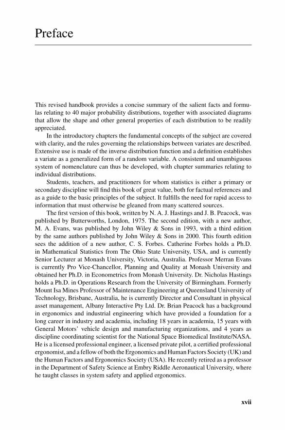
A random variable is a function that maps events defined on a sample space into aset of values. Several different random variables may be defined in relation to a givenexperiment. Thus, in the case of tossing two coins the number of heads observed isone random variable, the number of tails is another, and the number of double headsis another. The random variable “number of heads” associates the number 0 with theevent TT, the number 1 with the events TH and HT, and the number 2 with the eventHH. Figure 2.1 illustrates this mapping.
Variate
In the discussion of statistical distributions it is convenient to work in terms of vari-ates. A variate is a generalization of the idea of a random variable and has similar
Statistical Distributions, Fourth Edition, by Catherine Forbes, Merran Evans, Nicholas Hastings,and Brian PeacockCopyright © 2011 John Wiley & Sons, Inc.
3
4 Chapter 2 Terms and Symbols
Sample space
Hea
ds
TT TH HT HH
0
1
2
Figure 2.1. The random variable “number of heads”.
probabilistic properties but is defined without reference to a particular type of prob-abilistic experiment. A variate is the set of all random variables that obey a givenprobabilistic law. The number of heads and the number of tails observed in indepen-dent coin tossing experiments are elements of the same variate since the probabilisticfactors governing the numerical part of their outcome are identical.
A multivariate is a vector or a set of elements, each of which is a variate. A matrixvariate is a matrix or two-dimensional array of elements, each of which is a variate.In general, dependencies may exist between these elements.
Random Number
A random number associated with a given variate is a number generated at a realizationof any random variable that is an element of that variate.
2.2 RANGE, QUANTILE, PROBABILITY STATEMENT,AND DOMAIN
Range
Let X denote a variate and let �X be the set of all (real number) values that the variatecan take. The set �X is the range of X. As an illustration (illustrations are in termsof random variables) consider the experiment of tossing two coins and noting thenumber of heads. The range of this random variable is the set {0, 1, 2} heads, sincethe result may show zero, one, or two heads. (An alternative common usage of theterm range refers to the largest minus the smallest of a set of variate values.)
2.3 Distribution Function and Survival Function 5
Quantile
For a general variate X let x (a real number) denote a general element of the range�X. We refer to x as the quantile of X. In the coin tossing experiment referred topreviously, x ∈ {0, 1, 2} heads; that is, x is a member of the set {0, 1, 2} heads.
Probability Statement
Let X = x mean “the value realized by the variate X is x.” Let Pr[X ≤ x] mean “theprobability that the value realized by the variate X is less than or equal to x.”
Probability Domain
Let α (a real number between 0 and 1) denote probability. Let �αX be the set of all
values (of probability) that Pr[X ≤ x] can take. For a continuous variate, �αX is the
line segment [0, 1]; for a discrete variate it will be a subset of that segment. Thus �αX
is the probability domain of the variate X.In examples we shall use the symbol X to denote a random variable. Let X be
the number of heads observed when two coins are tossed. We then have
Pr[X ≤ 0] = 1
4
Pr[X ≤ 1] = 3
4Pr[X ≤ 2] = 1
and hence �αX = { 1
4 , 34 , 1}.
2.3 DISTRIBUTION FUNCTION AND SURVIVALFUNCTION
Distribution Function
The distribution function F (or more specifically FX) associated with a variate X
maps from the range �X into the probability domain �αX or [0, 1] and is such that
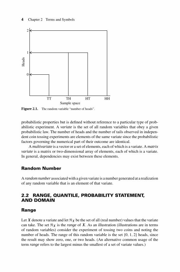
F (x) = Pr[X ≤ x] = α x ∈ �X, α ∈ �αX. (2.1)
The function F (x) is nondecreasing in x and attains the value unity at the maximumof x. Figure 2.2 illustrates the distribution function for the number of heads in the ex-periment of tossing two coins. Figure 2.3 illustrates a general continuous distributionfunction and Figure 2.4 a general discrete distribution function.

6 Chapter 2 Terms and Symbols
Quantile x
Prob
abili
ty α
10 2
0.25
0.5
0.75
1
Figure 2.2. The distribution function F : x → α or α = F (x) for the random variable, “number ofheads”.
1
0 x = G(α)
α = F(x)
Prob
abili
ty α
Quantile x
Figure 2.3. Distribution function and inverse distribution function for a continuous variate.
Survival Function
The survival function S(x) is such that
S(x) = Pr[X > x] = 1 − F (x).
2.4 Inverse Distribution Function and Inverse Survival Function 7
1
0
Prob
abili
ty α
Quantile x
x = G(α)
α = F(x)
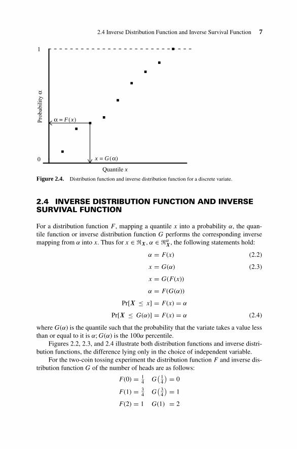
Figure 2.4. Distribution function and inverse distribution function for a discrete variate.
2.4 INVERSE DISTRIBUTION FUNCTION AND INVERSESURVIVAL FUNCTION
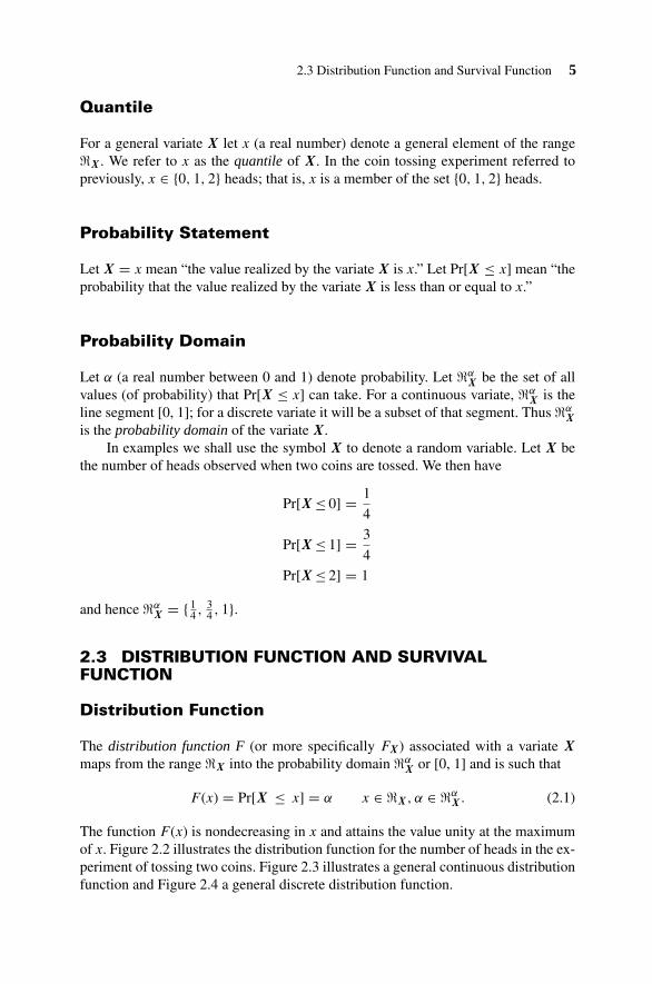
For a distribution function F , mapping a quantile x into a probability α, the quan-tile function or inverse distribution function G performs the corresponding inversemapping from α into x. Thus for x ∈ �X, α ∈ �α
X, the following statements hold:
α = F (x) (2.2)
x = G(α) (2.3)
x = G(F (x))
α = F (G(α))
Pr[X ≤ x] = F (x) = α
Pr[X ≤ G(α)] = F (x) = α (2.4)
where G(α) is the quantile such that the probability that the variate takes a value lessthan or equal to it is α; G(α) is the 100α percentile.
Figures 2.2, 2.3, and 2.4 illustrate both distribution functions and inverse distri-bution functions, the difference lying only in the choice of independent variable.
For the two-coin tossing experiment the distribution function F and inverse dis-tribution function G of the number of heads are as follows:
F (0) = 14 G
( 14
) = 0
F (1) = 34 G
( 34
) = 1
F (2) = 1 G(1) = 2

8 Chapter 2 Terms and Symbols
Inverse Survival Function
The inverse survival function Z is a function such that Z(α) is the quantile, which isexceeded with probability α. This definition leads to the following equations:
Pr[X > Z(α)] = α
Z(α) = G(1 − α)
x = Z(α) = Z(S(x))
Inverse survival functions are among the more widely tabulated functions in statistics.For example, the well-known chi-squared tables are tables of the quantile x as afunction of the probability level α and a shape parameter, and hence are tables of thechi-squared inverse survival function.
2.5 PROBABILITY DENSITY FUNCTION ANDPROBABILITY FUNCTION
A probability density function, f (x), is the first derivative coefficient of a distributionfunction, F (x), with respect to x (where this derivative exists).
f (x) = d(F (x))
dx
For a given continuous variate X the area under the probability density curve betweentwo points xL, xU in the range of X is equal to the probability that an as-yet unrealizedrandom number of X will lie between xL and xU . Figure 2.5 illustrates this. Figure 2.6
xL xU
Area is Prob(xL < X ≤ xU) = ⌠⌡xL
xUf (x)dx
Prob
abili
ty d
ensi
ty f
(x)
Quantile x
Figure 2.5. Probability density function.
2.6 Other Associated Functions and Quantities 9
G(α)
Prob
abili
ty d
ensi
ty f
(x)
Quantile x
Area α
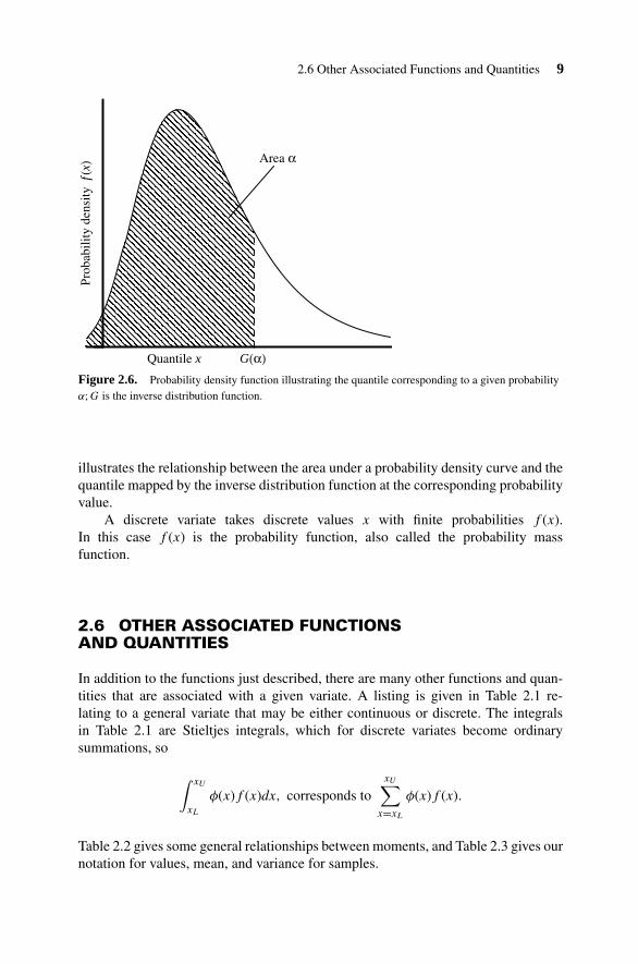
Figure 2.6. Probability density function illustrating the quantile corresponding to a given probabilityα; G is the inverse distribution function.
illustrates the relationship between the area under a probability density curve and thequantile mapped by the inverse distribution function at the corresponding probabilityvalue.
A discrete variate takes discrete values x with finite probabilities f (x).In this case f (x) is the probability function, also called the probability massfunction.
2.6 OTHER ASSOCIATED FUNCTIONSAND QUANTITIES
In addition to the functions just described, there are many other functions and quan-tities that are associated with a given variate. A listing is given in Table 2.1 re-lating to a general variate that may be either continuous or discrete. The integralsin Table 2.1 are Stieltjes integrals, which for discrete variates become ordinarysummations, so
∫ xU
xL
φ(x)f (x)dx, corresponds toxU∑
x=xL
φ(x)f (x).
Table 2.2 gives some general relationships between moments, and Table 2.3 gives ournotation for values, mean, and variance for samples.

10 Chapter 2 Terms and Symbols
Table 2.1: Functions and Related Quantities for a General Variate (X Denotes a Variate, x aQuantile, and α a Probability)
Term Symbol Description and notes
1. Distribution function (df) orcumulative distributionfunction (cdf)
F (x) F (x) is the probability that the variate takesa value less than or equal to x.
F (x) = Pr[X ≤ x] = α
F (x) =∫ x
−∞f (u) du
2. Probability density function(pdf) (continuous variates)
f (x) A function whose general integral over therange xL to xU is equal to the probabilitythat the variate takes a value in that range.∫ xU
xL
f (x) dx = Pr[xL < X ≤ xU ]
f (x) = d (F (x))
dx
3. Probability function (pf)(discrete variates)
f (x) f (x) is the probability that the variate takesthe value x.
f (x) = Pr[X = x]
4. Inverse distribution function orquantile function (ofprobability α)
G(α) G(α) is the quantile such that the probabilitythat the variate takes a value less than orequal to it is α.
x = G(α) = G(F (x))
Pr[X ≤ G(α)] = α
G(α) is the 100 α percentile. Therelation to df and pdf is shown inFigures 2.3, 2.4, and 2.6.
5. Survival function S(x) S(x) is the probability that the variate takesa value greater than x.
S(x) = Pr[X > x] = 1 − F (x)
6. Inverse survival function(of probability α)
Z(α) Z(α) is the quantile that is exceeded by thevariate with probability α.
Pr[X > Z(α)] = α
x = Z(α) = Z(S(x))
where S is the survival function
Z(α) = G(1 − α)
and G is the inverse distribution function.

2.6 Other Associated Functions and Quantities 11
Table 2.1: (Continued )
Term Symbol Description and notes
7. Hazard function (or failurerate, hazard rate, or force ofmortality)
h(x) h(x) is the ratio of the probability densityfunction to the survival function at quan-tile x.
h(x) = f (x)/S(x)
h(x) = f (x)/(1 − F (x))
8. Mills ratio m(x) m(x) is the inverse of the hazard function.
m(x) = (1 − F (x))/f (x) = 1/h(x)
9. Cumulative or integratedhazard function
H(x) Integral of the hazard function.
H(x) =∫ x
−∞h(u)du
H(x) = − log(1 − F (x))
S(x) = 1 − F (x) = exp(−H(x))
10. Probability generatingfunction (discrete nonnegativeinteger valued variates); alsocalled the geometric or z
transform
P(t) A function of an auxiliary variable t (or al-ternatively z) such that the coefficient oftx = f (x).
P(t) =∞∑
x=0
txf (x)
f (x) =(
1
x!
)(dxP(t)
dtx
)t=0
11. Moment generating function(mgf)
M(t) A function of an auxiliary variable t whosegeneral term is of the form μ′
rtr/r!.
M(t) =∫ ∞
−∞exp(tx)f (x)dx
M(t) = 1 + μ′1t + μ′
2t2/2!
+ · · · + μ′rt
r/r! + · · ·For any independent variates A and B,whose moment generating functionsMA(t) and MB(t) respectively, exist, thenthe mgf of A + B exists and satisfies
MA+B(t) = MA(t)MB(t).
(continued )

12 Chapter 2 Terms and Symbols
Table 2.1: (Continued )
Term Symbol Description and notes
12. Laplace transform of the pdf f ∗(s) A function of the auxiliary variable s
defined by
f ∗(s) =∫ ∞
0
exp(−sx)f (x)dx, x≥0.
13. Characteristic function C(t) A function of the auxiliary variable t andthe imaginary quantity i (i2 = −1), whichexists and is unique to a given pdf.
C(t) =∫ +∞
−∞exp(itx)f (x)dx
If C(t) is expanded in powers of t and if μ′r
exists, then the general term is μ′r(it)
r/r!For any independent variates A and B
CA+B(t) = CA(t)CB(t)
14. Cumulant generationfunction
K(t) K(t) = log C(t) [sometimes definedlog M(t)].
KA+B(t) = KA(t) + KB(t)
15. rth Cumulant kr The coefficient of (it)r/r! in the expansionof K(t).
16. rth Moment about the origin μ′r μ′
r =∫ ∞
−∞xrf (x)dx
μ′r =
(drM(t)
dtr
)t=0
μ′r = (−i)r
(drC(t)
dtr
)t=0
17. Mean (first moment about theorigin)
μ μ =∫ +∞
−∞xf (x)dx = μ′
1
18. rth (Central) moment aboutthe mean
μr μr =∫ +∞
−∞(x − μ)rf (x)dx
19. Variance (second momentabout the mean, μ2)
σ2 σ2 =∫ +∞
−∞(x − μ)2f (x)dx
= μ2 = μ′2 − μ2

2.6 Other Associated Functions and Quantities 13
Table 2.1: (Continued )
Term Symbol Description and notes
20. Standard deviation σ The positive square root of the variance.
21. Mean deviation∫ +∞
−∞ |x − μ|f (x)dx. The mean absolutevalue of the deviation from the mean.
22. Mode A quantile for which the pdf or pf is a localmaximum.
23. Median m The quantile that is exceeded withprobability 1
2 , m = G( 12 ).
24. Quartiles The upper and lower quartiles are exceededwith probabilities 1
4 and 34 ,
corresponding to G( 14 ) and G( 3
4 ),respectively.
25. Percentiles G(α) is the 100 α percentile.
26. Standardized rth moment ηr The rth moment about the meanabout the mean scaled so that the standard deviation is
unity.
ηr =∫ +∞
−∞
(x − μ
σ
)r
f (x)dx = μr
σr
27. Coefficient of skewness η3√
β1 = η3 = μ3/σ3 = μ3/μ
3/22
28. Coefficient of kurtosis η4 β2 = η4 = μ4/σ4 = μ4/μ
22
Coefficient of excess or excesskurtosis is β2 − 3; β2<3 is platykurtosis;β2 > 3 is leptokurtosis.
29. Coefficient of variation Standard deviation/mean = σ/μ.
30. Information content (orentropy)
l l = − ∫ +∞−∞ f (x) log2(f (x))dx
31. rth Factorial moment aboutthe origin (discretenonnegative variates)
μ′(r)
∞∑x=0
f (x) · x(x − 1)(x − 2)
· · · (x − r + 1)
μ′(r) = (
drP(t)dtr
)t=1
(continued )

14 Chapter 2 Terms and Symbols
Table 2.1: (Continued )
Term Symbol Description and notes
32. rth Factorial moment aboutthe mean (discretenonnegative variate)
μ(r)
∞∑x=0
f (x) · (x − μ)(x − μ − 1) · · ·
(x − μ − r + 1)
Table 2.2: General Relationships Between Moments
Moments about the origin μ′r =
r∑i=0
(r
i
)μr−i(μ′
1)i, μ0 = 1
Central moments about mean μr =r∑
i=0
(r
i
)μ′
r−i(−μ′1)i, μ′
0 = 1
Hence,
μ2 = μ′2 − μ
′21
μ3 = μ′3 − 3μ′
2μ′1 + 2μ
′31
μ4 = μ′4 − 4μ′
3μ′1 + 6μ′
2μ′21 − 3μ
′41
Moments and cumulants μ′r =
r∑i=1
(r − 1i − 1
)μ′
r−iκi
Table 2.3: Samples
Term Symbol Description and notes
Sample data xi xi is an observed value of a randomvariable.
Sample size n The number of observations in a sample.
Sample mean x 1n
n∑i=1
xi
Sample variance (unadjusted for bias) s2 1n
n∑i=1
(xi − x)2
Sample variance (unbiased) s2u
(1
n−1
) n∑i=1
(xi − x)2
Chapter 3
General Variate Relationships
3.1 INTRODUCTION
This chapter is concerned with general relationships between variates and with theideas and notation needed to describe them. Some definitions are given, and therelationships between variates under one-to-one transformations are developed. Lo-cation, scale, and shape parameters are then introduced, and the relationships betweenfunctions associated with variates that differ only in regard to location and scale arelisted. The relationship of a general variate to the rectangular variate is derived, andfinally the notation and concepts involved in dealing with variates that are related bymany-to-one functions and by functionals are discussed.
Following the notation introduced in Chapter 2 we denote a general variate byX, its range by �X, its quantile by x, and a realization or random number of X by xX.
3.2 FUNCTION OF A VARIATE
Let φ be a function mapping from �X into a set we shall call �φ(X).
Definition 3.2.1 (Function of a Variate). The term φ(X) is a variate such that ifxX is a random number of X then φ(xX) is a random number of φ(X).
Thus a function of a variate is itself a variate whose value at any realization is obtainedby applying the appropriate transformation to the value realized by the original variate.For example, if X is the number of heads obtained when three coins are tossed, thenX3 is the cube of the number of heads obtained. (Here, as in Chapter 2, we usethe symbol X for both a variate and a random variable that is an element of thatvariate.)
The probabilistic relationship between X and φ(X) will depend on whether morethan one number in �X maps into the same φ(x) in �φ(X). That is, it is important toconsider whether φ is or is not a one-to-one function over the range considered. Thispoint is taken up in Section 3.3.
Statistical Distributions, Fourth Edition, by Catherine Forbes, Merran Evans, Nicholas Hastings,and Brian PeacockCopyright © 2011 John Wiley & Sons, Inc.
15

16 Chapter 3 General Variate Relationships
A definition similar to 3.2.1 applies in the case of a function of several variates;we shall detail the case of a function of two variates. Let X, Y be variates with ranges�X, �Y and let ψ be a functional mapping from the Cartesian product of �X and �Y
into (all or part of) the real line.
Definition 3.2.2 (Function of Two Variates). The term ψ(X, Y ) is a variate suchthat if xX and xY are random numbers of X and Y , respectively, then φ(xX, xY ) is arandom number of ψ(X, Y ).
3.3 ONE-TO-ONE TRANSFORMATIONS AND INVERSES
Let φ be a function mapping from the real line into the real line.
Definition 3.3.1 (One-to-One Function). The function φ is one to one if there areno two numbers x1, x2 in the domain of φ such that φ(x1) = φ(x2) and x1 /= x2.
A sufficient condition for a real function to be one to one is that it be increasing in x.As an example, φ(x) = exp(x) is a one-to-one function, but φ(x) = x2 is not (unless x
is confined to all negative or all positive values, say) since x1 = 2 and x2 = −2 givesφ(x1) = φ(x2) = 4. Figures 3.1 and 3.2 illustrate this. A function that is not one toone is a many-to-one function. See also Section 3.8.
x1 x2 x
φ( x ) = exp (x )
φ(x1)
φ(x2)
φ(x)
Figure 3.1. A one-to-one function.

3.4 Variate Relationships Under One-to-One Transformation 17
x1 x2 x
φ(x1) = φ(x2)
φ(x)
Figure 3.2. A many-to-one function.
Inverse of a One-to-One Function
The inverse of a one-to-one function φ is a one-to-one function φ−1, where
φ−1(φ(x)) = x, φ(φ−1(y)) = y (3.1)
and x and y are real numbers (Bernstein’s Theorem).
3.4 VARIATE RELATIONSHIPS UNDER ONE-TO-ONETRANSFORMATION
Probability Statements
Definitions 3.2.1 and 3.3.1 imply that if X is a variate and φ is an increasing one-to-onefunction, then φ(X) is a variate with the property
Pr[X ≤ x] = Pr[φ(X) ≤ φ(x)]
x ∈ �X; φ(x) ∈ �φ(X).(3.2)
Distribution Function
In terms of the distribution function FX(x) for variate X at quantile x, Equation (3.2)is equivalent to the statement
FX(x) = Fφ(X)(φ(x)). (3.3)

18 Chapter 3 General Variate Relationships
To illustrate Equations (3.2) and (3.3) consider the experiment of tossing threecoins and the random variables “number of heads,” denoted by X, and “cube ofthe number of heads,” denoted by X3. The probability statements and distributionfunctions at quantiles 2 heads and 8 (heads)3 are
Pr[X≤2] = Pr[X3≤8] = 78
FX(2) = FX3 (8) = 78 .
(3.4)
Inverse Distribution Function
The inverse distribution function (introduced in Section 2.4) for a variate X at proba-bility level α is GX(α). For a one-to-one function φ we now establish the relationshipbetween the inverse distribution functions of the variates X and φ(X).
Theorem 3.4.1.
φ(GX(α)) = Gφ(X)(α).
Proof Equations (2.4) and (3.3) imply that if
GX(α) = x then Gφ(X)(α) = φ(x)
which implies that the theorem is true. �
We illustrate this theorem by extending the example of Equation (3.4). Consid-ering the inverse distribution function, we have
GX
(7
8
)= 2; GX3
(7
8
)= 8 = 23 =
(GX
(7
8
))3
.
Equivalence of Variates
For any two variates X and Y , the statement X ∼ Y , read “X is distributed as Y ,”means that the distribution functions of X and Y are identical. All other associatedfunctions, sets, and probability statements of X and Y are therefore also identical. “Isdistributed as” is an equivalent relation, so that
1. X ∼ X.
2. X ∼ Y implies Y ∼ X.
3. X ∼ Y and Y ∼ Z implies X ∼ Z.
Inverse Function of a Variate
Theorem 3.4.2. If X and Y are variates and φ is an increasing one-to-one function,then Y ∼ φ(X) implies φ−1(Y ) ∼ X.
3.5 Parameters, Variate, and Function Notation 19
Proof
Y ∼ φ(X) implies Pr[Y ≤ x] = Pr[φ(X) ≤ x]
(by the equivalence of variates, above)
Pr[Y ≤ x] = Pr[X ≤ φ−1(x)]
= Pr[φ−1(Y ) ≤ φ−1(x)]
(from Equations (3.1) and (3.2)).These last two equations together with the equivalence of variates (above) imply
that Theorem 3.4b is true. �
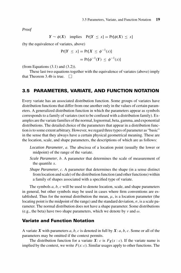
3.5 PARAMETERS, VARIATE, AND FUNCTION NOTATION
Every variate has an associated distribution function. Some groups of variates havedistribution functions that differ from one another only in the values of certain param-eters. A generalized distribution function in which the parameters appear as symbolscorresponds to a family of variates (not to be confused with a distribution family). Ex-amples are the variate families of the normal, lognormal, beta, gamma, and exponentialdistributions. The detailed choice of the parameters that appear in a distribution func-tion is to some extent arbitrary. However, we regard three types of parameter as “basic”in the sense that they always have a certain physical geometrical meaning. These arethe location, scale, and shape parameters, the descriptions of which are as follows:
Location Parameter, a. The abscissa of a location point (usually the lower ormidpoint) of the range of the variate.
Scale Parameter, b. A parameter that determines the scale of measurement ofthe quantile x.
Shape Parameter, c. A parameter that determines the shape (in a sense distinctfrom location and scale) of the distribution function (and other functions) withina family of shapes associated with a specified type of variate.
The symbols a, b, c will be used to denote location, scale, and shape parametersin general, but other symbols may be used in cases where firm conventions are es-tablished. Thus for the normal distribution the mean, μ, is a location parameter (thelocating point is the midpoint of the range) and the standard deviation, σ, is a scale pa-rameter. The normal distribution does not have a shape parameter. Some distributions(e.g., the beta) have two shape parameters, which we denote by ν and ω.
Variate and Function Notation
A variate X with parameters a, b, c is denoted in full by X: a, b, c. Some or all of theparameters may be omitted if the context permits.
The distribution function for a variate X: c is FX(x : c). If the variate name isimplied by the context, we write F (x: c). Similar usages apply to other functions. The

20 Chapter 3 General Variate Relationships
inverse distribution function for a variate X: a, b, c at probability level α is denotedGX(α : a, b, c).
3.6 TRANSFORMATION OF LOCATION AND SCALE
Let X: 0, 1 denote a variate with location parameter a = 0 and scale parameter b = 1.(This is often referred to as the standard variate.) A variate that differs from X: 0, 1only in regard to location and scale is denoted X: a, b and is defined by
X : a, b ∼ a + b(X : 0, 1). (3.5)
The location and scale transformation function is the one-to-one function
φ(x) = a + bx
and its inverse is
φ−1(x) = (x − a)/b
with b /= 0. (Typically b > 0.)The following equations relating to variates that differ only in relation to location andscale parameters then hold:
X : a, b ∼ a + b(X : 0, 1)
(by definition)
X : 0, 1 ∼ [(X : a, b) − a]/b
(by Theorem 3.4.2 and Equation (3.5)]
Pr[(X : a, b) ≤ x] = Pr[(X : 0, 1) ≤ (x − a)/b]
(by Equation (3.2)) (3.6)
FX(x : a, b) = FX{[(x − a)/b] : 0, 1}(equivalent to Equation (3.6))
GX(α : a, b) = a + b(GX(α : 0, 1))
(by Theorem 3.4.1)
These and other interrelationships between functions associated with variates thatdiffer only in regard to location and scale parameters are summarized in Table 3.1.The functions themselves are defined in Table 2.1.
3.7 TRANSFORMATION FROM THE RECTANGULARVARIATE
The following transformation is often useful for obtaining random numbers of a variateX from random numbers of the unit rectangular variate R. The latter has distribution

3.8 Transformation from the Rectangular Variate 21
Table 3.1: Relationships Between Functions for Variates that Differ Only by Location andScale Parameters a, b
Variate relationship X: a, b ∼ a + b(X : 0, 1)
Probability statement Pr[(X : a, b) ≤ x] = Pr[(X : 0, 1) ≤ (x − a)/b]
Function relationships
Distribution function F (x : a, b) = F ([(x − a)/b] : 0, 1)
Probability density function f (x : a, b) = (1/b)f ([(x − a)/b] : 0, 1)
Inverse distribution function G(α : a, b) = a + bG(α : 0, 1)
Survival function S(x : a, b) = S([(x − a)/b] : 0, 1)
Inverse survival function Z(α : a, b) = a + bZ(α : 0, 1)
Hazard function h(x : a, b) = (1/b)h([(x − a)/b] : 0, 1)
Cumulative hazard function H(x : a, b) = H([(x − a)/b] : 0, 1)
Moment generating function M(t : a, b) = exp(at)M(bt : 0, 1)
Laplace transform f ∗(s : a, b) = exp(−as)f ∗(bs : 0, 1), a > 0
Characteristic function C(t : a, b) = exp(iat)C(bt : 0, 1)
Cumulant function K(t : a, b) = iat + K(bt : 0, 1)
function FR(x) = x, 0 ≤ x ≤ 1, and inverse distribution function GR(α) = α, 0 ≤α ≤ 1. The inverse distribution function of a general variate X is denoted GX(α), α ∈�a
X. Here GX(α) is a one-to-one function.
Theorem 3.7.1. X ∼ GX(R) for continuous variates.
Proof
Pr[R ≤ α] = α, 0 ≤ α ≤ 1
(property of R)
= Pr[GX(R) ≤ GX(α)]
(by Equation (3.2))
Hence, by these two equations and Equation (2.4),
GX(R) ∼ X. �
For discrete variates, the corresponding expression is
X ∼ GX[f (R)], where f (α) = Min{p|p ≥ α, p ∈ �αX}.
Thus every variate is related to the unit rectangular variate via its inverse distributionfunction, although, of course, this function will not always have a simple algebraicform.

22 Chapter 3 General Variate Relationships
3.8 MANY-TO-ONE TRANSFORMATIONS
In Sections 3.3 through 3.7 we considered the relationships between variates that werelinked by a one-to-one function. Now we consider many-to-one functions, which aredefined as follows. Let φ be a function mapping from the real line into the real line.
Definition 3.8.1 (Many-to-One Function). The function φ is many to one if thereare at least two numbers x1, x2 in the domain of φ such that φ(x1) = φ(x2), x1 /= x2.
The many-to-one function φ(x) = x2 is illustrated in Figure 3.2.In Section 3.2 we defined, for a general variate X with range �X and for a function
φ, a variate φ(X) with range �φ(X). Here φ(X) has the property that if xX is a randomnumber of X, then φ(xX) is a random number of φ(X). Let r2 be a subset of �φ(X)and r1 be the subset of �X, which φ maps into r2. The definition of φ(X) implies that
Pr[X ∈ r1] = Pr[φ(X) ∈ r2].
This equation enables relationships between X and φ(X) and their associated func-tions to be established. If φ is many-to-one, the relationships will depend on thedetailed form of φ.
EXAMPLE 3.8.1
As an example we consider the relationships between the variates X and X2 for the case where�X is the real line. We know that φ : x → x2 is a many-to-one function. In fact it is a two-to-onefunction in that +x and −x both map into x2. Hence the probability that an as-yet unrealizedrandom number of X2 will be greater than x2 will be equal to the probability that an as-yetunrealized random number of X will be either greater than +|x| or less than −|x|.
Pr[X2 > x2] = Pr[X > +|x|] + Pr[X] < −|x|]. (3.7)
Symmetrical Distributions
Let us now consider a variate X whose probability density function is symmetricalabout the origin. We shall derive a relationship between the distribution function ofthe variates X and X2 under the condition that X is symmetrical. An application ofthis result appears in the relationship between the F (variance ratio) and Student’st variates.
Theorem 3.8.1. Let X be a variate whose probability density function is symmetricalabout the origin.
1. The distribution functions FX(x) and FX2 (x2) for the variates X and X2 atquantiles x ≥ 0 and x2, respectively, are related by
FX(x) = 12
[1 + FX2 (x2)
]
3.8 Many-to-One Transformations 23
or
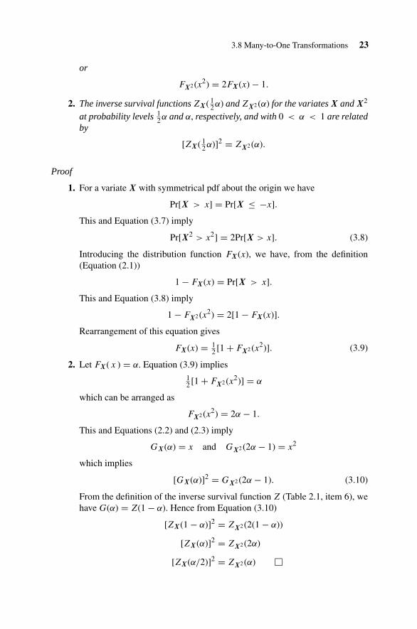
FX2 (x2) = 2FX(x) − 1.
2. The inverse survival functions ZX( 12α) and ZX2 (α) for the variates X and X2
at probability levels 12α and α, respectively, and with 0 < α < 1 are related
by
[ZX( 12α)]2 = ZX2 (α).
Proof
1. For a variate X with symmetrical pdf about the origin we have
Pr[X > x] = Pr[X ≤ −x].
This and Equation (3.7) imply
Pr[X2 > x2] = 2Pr[X > x]. (3.8)
Introducing the distribution function FX(x), we have, from the definition(Equation (2.1))
1 − FX(x) = Pr[X > x].
This and Equation (3.8) imply
1 − FX2 (x2) = 2[1 − FX(x)].
Rearrangement of this equation gives
FX(x) = 12 [1 + FX2 (x2)]. (3.9)
2. Let FX( x ) = α. Equation (3.9) implies12 [1 + FX2 (x2)] = α
which can be arranged as
FX2 (x2) = 2α − 1.
This and Equations (2.2) and (2.3) imply
GX(α) = x and GX2 (2α − 1) = x2
which implies
[GX(α)]2 = GX2 (2α − 1). (3.10)
From the definition of the inverse survival function Z (Table 2.1, item 6), wehave G(α) = Z(1 − α). Hence from Equation (3.10)
[ZX(1 − α)]2 = ZX2 (2(1 − α))
[ZX(α)]2 = ZX2 (2α)
[ZX(α/2)]2 = ZX2 (α) �
Chapter 4
Multivariate Distributions
4.1 JOINT DISTRIBUTIONS
Probability statements concerning more than one random variate are called jointprobability statements. Joint probability statements can be made about a combinationof variates, all having continuous domain, all having countable domain, or somecombination of continuous and countable domains.
To keep notation to a minimum, consider the case of only two variates, X andY , and call the pair (X, Y ) a bivariate, with each of X and Y alone referred to asunivariates. In the general case of more than one variate (including the bivariatecase), the collection of variates is more generally referred to as a multivariate.
Joint Range
Let �X,Y be the set of all pairs of (real number) values that the bivariate (X, Y ) cantake. The set �X,Y is the joint range of (X, Y ).
Bivariate Quantile
Let the real valued pair (x, y) denote a general element of the joint range �X,Y . Werefer to (x, y) as a bivariate quantile of (X, Y ).
Joint Probability Statement
Let Pr[X ≤ x, Y ≤ y] mean “the probability that the value realized by the univariateX is less than or equal to x and the value realized by the univariate Y is less than orequal to y.” In this case, both conditions X ≤ x and Y ≤ y hold simultaneously.
Statistical Distributions, Fourth Edition, by Catherine Forbes, Merran Evans, Nicholas Hastings,and Brian PeacockCopyright © 2011 John Wiley & Sons, Inc.
24

4.1 Joint Distributions 25
Joint Probability Domain
Let α ∈ [0, 1] and let �αX,Y be the set of all values (of probability) that Pr[X ≤
x, Y ≤ y] can take. When X and Y are jointly continuous, �αX,Y is the line segment
[0, 1]. In all other cases, �αX,Y may be a subset of [0, 1]. Analogous to the univariate
case, �αX,Y is called the joint probability domain of the bivariate (X, Y ).
Joint Distribution Function
The distribution function (joint df) F associated with a bivariate (X, Y ) maps fromthe joint range �X,Y into the joint probability domain �α
X,Y and is such that
F (x, y) = Pr[X ≤ x, Y ≤ y] = α, for (x, y) ∈ �X,Y , α ∈ �αX,Y .
The function F (x, y) is nondecreasing in each of x and y, and attains a value of unitywhen both x and y are at their respective maxima.
Joint Probability Density Function
When (X, Y ) have a jointly continuous probability domain, the function f (x, y) is abivariate probability density function (joint pdf) if
F (x, y) =∫ y
−∞
∫ x
−∞f
(ux, uy
)dux duy
for all (x, y) in �X,Y . This relationship implies that the pdf satisfies
f (x, y) = ∂2F (x, y)
∂x ∂y
and that the probability associated with an arbitrary bivariate quantile set A is equalto the area under the bivariate pdf surface A. That is,
Pr[(x, y) ∈ A] =∫∫
(x,y)∈A
f (x, y) dx dy.
Joint Probability Function
A discrete bivariate (X, Y ) takes discrete values (x, y) with finite probabilities f (x, y).In this case f (x, y) is the bivariate probability function (joint pf).

26 Chapter 4 Multivariate Distributions
Table 4.1: Joint Probability Function for Discrete Bivariate Example
Pr [X = 0, Y = 0] = 1/8 Pr [X = 0, Y = 1] = 1/8
Pr [X = 1, Y = 0] = 3/8 Pr [X = 1, Y = 1] = 1/8
Pr [X = 2, Y = 0] = 3/16 Pr [X = 2, Y = 1] = 1/16
EXAMPLE 4.1.1. Discrete Bivariate
Consider the discrete bivariate (X, Y ) with joint distribution function given by
F (x, y) =
⎧⎪⎪⎪⎪⎪⎪⎪⎪⎪⎪⎪⎪⎪⎨⎪⎪⎪⎪⎪⎪⎪⎪⎪⎪⎪⎪⎪⎩
0 x < 0, y < 0
1/8 0 ≤ x < 1, 0 ≤ y < 1
1/4 0 ≤ x < 1, y ≥ 1
1/2 1 ≤ x < 2, 0 ≤ y < 1.
3/4 1 ≤ x < 2, y ≥ 1
11/16 x ≥ 2, 0 ≤ y < 1
1 x ≥ 2, y ≥ 1.
As the joint distribution function changes only when x reaches zero, one or two, and wheny reaches zero or one, the joint range is �X,Y = {(0, 0) , (1, 0) , (2, 0) , (0, 1) , (1, 1) , (1, 2)}.The resulting joint pf is given in Table 4.1. In this case the joint probability domain is �α
X,Y ={18 , 1
4 , 12 , 3
4 , 1116 , 1
}.
4.2 MARGINAL DISTRIBUTIONS
Probabilities associated with a univariate element of a bivariate without regard to thevalue of the other univariate element within the same bivariate arise from the marginaldistribution of that univariate. Corresponding to such a marginal distribution are the(univariate) range, quantile, and probability domain associated with the univariateelement, with each one consistent with the corresponding bivariate entity.
Marginal Probability Density Function and MarginalProbability Function
In the case of continuous bivariate (X, Y ) having joint pdf f (x, y), the marginalprobability density function (marginal pdf) of the univariate X is found for eachquantile x by integrating the joint pdf over all possible bivariate quantiles (x, y) ∈�X,Y having fixed value for x,
f (x) =∫ ∞
−∞f (x, y) dy.
4.3 Independence 27
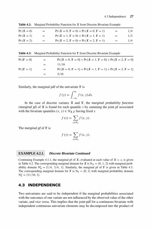
Table 4.2: Marginal Probability Function for X from Discrete Bivariate Example
Pr (X = 0) = Pr (X = 0, Y = 0) + Pr (X = 0, Y = 1) = 1/4
Pr (X = 1) = Pr (X = 1, Y = 0) + Pr (X = 1, Y = 1) = 1/2
Pr (X = 2) = Pr (X = 2, Y = 0) + Pr (X = 2, Y = 1) = 1/4
Table 4.3: Marginal Probability Function for Y from Discrete Bivariate Example
Pr [Y = 0] = Pr [X = 0, Y = 0] + Pr [X = 1, Y = 0] + Pr [X = 2, Y = 0]
= 11/16
Pr [Y = 1] = Pr [X = 0, Y = 1] + Pr [X = 1, Y = 1] + Pr [X = 2, Y = 1]
= 5/16
Similarly, the marginal pdf of the univariate Y is
f (y) =∫ ∞
−∞f (x, y) dx.
In the case of discrete variates X and Y , the marginal probability function(marginal pf) of X is found for each quantile x by summing the joint pf associatedwith the bivariate quantiles (x, y) ∈ �X,Y having fixed x
f (x) =∑y∈�y
f (x, y) .
The marginal pf of Y is
f (y) =∑x∈�x
f (x, y) .
EXAMPLE 4.2.1. Discrete Bivariate Continued
Continuing Example 4.1.1, the marginal pf of X, evaluated at each value of X = x, is givenin Table 4.2. The corresponding marginal domain for X is �X = {0, 1, 2} with marginal prob-ability domain �α
X = {1/4, 3/4, 1}. Similarly, the marginal pf of Y is given in Table 4.3.The corresponding marginal domain for Y is �Y = {0, 1} with marginal probability domain�α
Y = {11/16, 1}.
4.3 INDEPENDENCE
Two univariates are said to be independent if the marginal probabilities associatedwith the outcomes of one variate are not influenced by the observed value of the othervariate, and vice versa. This implies that the joint pdf for a continuous bivariate withindependent continuous univariate elements may be decomposed into the product of

28 Chapter 4 Multivariate Distributions
the marginal pdfs. Similarly, the joint pf for a discrete bivariate with independentdiscrete univariate elements may be decomposed into the product of the marginal pfs.That is,
f (x, y) = f (x) f (y) for all (x, y) ∈ �X,Y .
4.4 CONDITIONAL DISTRIBUTIONS
When two univariates are not independent, they are said to be dependent. In this case,interest often focuses on computing probabilities associated with one variate giveninformation about the realized value of the other variate. Such probabilities are calledconditional probabilities. For example, the “conditional probability that X is less thanx, given it is known that Y is less than y” is
Pr[X ≤ x|Y ≤ y] = Pr[X ≤ x, Y ≤ y]
Pr[Y ≤ y]
provided the denominator Pr[Y ≤ y] is nonzero.
Conditional Probability Function and ConditionalProbability Density Function
When conditioning on a single observed value of one univariate component Y = y
of a discrete bivariate (X, Y ), the conditional pf of X, given Y = y, and denoted byf (x|y), is found by taking the ratio of the joint pf f (x, y) to the marginal pf of Y ,f (y), for fixed Y = y
f (x|y) = Pr[X = x, Y = y]
Pr[Y = y]= f (x, y)
f (y),
for all (x, y) ∈ �X,Y . Similarly,
f (y|x) = Pr[X = x, Y = y]
Pr [X = x]for all (x, y) ∈ �X,Y .
For continuous random variates, the conditional probability density function (condi-tional pdf) for X given Y = y and denoted by f (x|y) may be constructed using theratio of the joint pdf over the marginal pdf of Y , for fixed Y = y
f (x|y) = f (x, y)
f (y)for all (x, y) ∈ �X,Y ,
for all (x, y) ∈ �X,Y . Similarly,
f (y|x) = f (x, y)
f (x)for all (x, y) ∈ �X,Y .

4.4 Conditional Distributions 29
Composition
Joint, marginal, and conditional probabilities satisfy the property of composition,whereby joint probabilities may be determined by the product of marginal probabili-ties and the appropriate conditional probability
Pr[X ≤ x, Y ≤ y] = Pr[X ≤ x|Y ≤ y]Pr[Y ≤ y].
The composition property implies joint, marginal, and conditional pdfs (or pfs)satisfy
f (x, y) = f (x|y) f (y) = f (y|x) f (x) for all (x, y) ∈ �X,Y . (4.1)
Equation (4.1) holds whether the variables are dependent or independent. However,if X and Y are independent, then f (y|x) = f (y) and f (x|y) = f (x), and hence
f (x, y) = f (x)f (y).
EXAMPLE 4.4.1. Discrete Bivariate Continued
Again continuing Example 4.1.1 the conditional pf of X, given Y = 0, is found by consideringthe individual joint probabilities in Table 4.1 and dividing by the marginal probability thatY = 0 from Table 4.3. The resulting conditional probabilities are
Pr[X = 0|Y = 0] = Pr[X = 0, Y = 0]
Pr[Y = 0]= 1/8
11/16= 2/11
Pr[X = 1|Y = 0] = Pr[X = 1, Y = 0]
Pr[Y = 0]= 3/8
11/16= 6/11
Pr[X = 2|Y = 0] = Pr[X = 2, Y = 0]
Pr[Y = 0]= 3/16
11/16= 3/11.
These conditional probabilities associated with the univariate X given Y = 0 are not thesame as those obtain by conditioning on a value of Y = 1, since
Pr[X = 0|Y = 1] = Pr[X = 0, Y = 1]
Pr[Y = 1]= 1/8
5/16= 2/5
Pr[X = 1|Y = 1] = Pr[X = 1, Y = 1]
Pr[Y = 1]= 1/8
5/16= 2/5
Pr[X = 2|Y = 1] = Pr[X = 2, Y = 1]
Pr[Y = 1]= 1/16
5/16= 1/5.
The conditional probabilities for Y given X = x are similarly found, with
Pr[Y = 0|X = 0] = 1/2
Pr[Y = 1|X = 0] = 1/2
Pr[Y = 0|X = 1] = 3/4
Pr[Y = 1|X = 1] = 1/4

30 Chapter 4 Multivariate Distributions
and
Pr[Y = 0|X = 2] = 3/4
Pr[Y = 1|X = 2] = 1/4.
Note, however, that composition may be used to reconstruct the joint probabilities for(X, Y ), for example, with
Pr[X = 0, Y = 1] = Pr[X = 0|Y = 1] Pr[Y = 1] = 2
5× 5
16= 1
8,
concurring with Pr[X = 0, Y = 1] in Table 4.1.
4.5 BAYES’ THEOREM
A fundamental result concerning conditional probabilities is known as Bayes’ theo-rem, providing the rule for reversing the roles of variates in a conditional probability.Bayes’ theorem states
f (y|x) = f (x|y)f (y)
f (x). (4.2)
For a continuous bivariate, the terms denoted by f (·) in Equation (4.2) relate tomarginal and conditional pdfs, whereas for a discrete bivariate these terms relate tomarginal and conditional pfs.
EXAMPLE 4.5.1. Discrete Bivariate Continued
Using Bayes’ theorem in Equation (4.2) relates the conditional probability Pr[X = x|Y = y]to the conditional probability Pr[Y = y|X = x], with
Pr[X = x|Y = y] = Pr[Y = y|X = x] Pr[X = x]
Pr[Y = y].
So, for example,
Pr[X = 2|Y = 0] = Pr[Y = 0|X = 2] Pr[X = 2]
Pr[Y = 0]
= (3/4) (1/4)
11/16= 3/11.
as before.
4.6 FUNCTIONS OF A MULTIVARIATE
If (X, Y ) is a bivariate with range �X,Y and ψ is a functional mapping from �X,Y
into the real line, then ψ(X, Y ) is a variate such that if xX and xY are random numbersof X and Y , respectively, then ψ(xX, xY ) is a random number of ψ(X, Y ).
The relationships between the associated functions of X and Y on the one handand of ψ(X, Y ) on the other are not generally straightforward and must be derived
4.6 Functions of a Multivariate 31
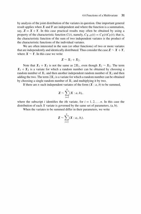
by analysis of the joint distribution of the variates in question. One important generalresult applies when X and Y are independent and where the function is a summation,say, Z = X + Y . In this case practical results may often be obtained by using aproperty of the characteristic function C(t), namely, CX+Y (t) = CX(t)CY (t); that is,the characteristic function of the sum of two independent variates is the product ofthe characteristic functions of the individual variates.
We are often interested in the sum (or other functions) of two or more variatesthat are independently and identically distributed. Thus consider the case Z ∼ X + Y ,where X ∼ Y . In this case we write
Z ∼ X1 + X2.
Note that X1 + X2 is not the same as 2X1, even though X1 ∼ X2. The termX1 + X2 is a variate for which a random number can be obtained by choosing arandom number of X1 and then another independent random number of X2 and thenadding the two. The term 2X1 is a variate for which a random number can be obtainedby choosing a single random number of X1 and multiplying it by two.
If there are n such independent variates of the form (X : a, b) to be summed,
Z ∼n∑
i=1
(X : a, b)i.
where the subscript i identifies the ith variate, for i = 1, 2, . . . n. In this case thedistribution of each X variate is governed by the same set of parameters, (a, b).
When the variates to be summed differ in their parameters, we write
Z ∼n∑
i=1
(X : ai, bi).

Chapter 5
Stochastic Modeling
5.1 INTRODUCTION
In this chapter we review the construction of a joint probability model for a sequenceof random variates, suitable for the description of observed data. Choosing a stochas-tic representation for observed data is arguably the most critical component of anystatistical exercise. In many cases the choice will be dictated by convention and con-venience, however, the implications of an incorrect model structure may be severe.
Before reviewing a few general approaches to specifying a stochastic model, it isworth pausing to consider one’s objective in modeling data. For example, is the maingoal to achieve a parsimonious description of the observed empirical distribution ofthe data? Is the prediction of future observations of interest? Alternatively, is thereinterest in testing whether the data are consistent with certain theoretical hypotheses?There may in fact be multiple objectives that one pursues when modeling data, but tosome degree the modeling method employed will be strongly influenced by the mainobjective.
5.2 INDEPENDENT VARIATES
If it is reasonable to assume that variates are independent of one another and thatthe marginal distribution for each variate is the same, then the variates are said to beindependent and identically distributed (i.i.d.). When variates X1, X2, . . . , Xn arei.i.d. the joint probability density function of the multivariate (X1, X2, . . . , Xn) isgiven by the product of the marginal univariate pdfs
f (x) =n∏
i=1
f (xi)
where x = (x1, x2, . . . , xn) denotes the multivariate quantile of X. Variates that arenot independent are said to be dependent. The modeling of dependent variates isdiscussed in Section 5.6.
Statistical Distributions, Fourth Edition, by Catherine Forbes, Merran Evans, Nicholas Hastings,and Brian PeacockCopyright © 2011 John Wiley & Sons, Inc.
32

5.3 Mixture Distributions 33
The marginal distribution function of i.i.d. variates each having distribution func-tion F , will be also be F . In this case, the empirical distribution function FE(x)(Chapter 14) will serve as a useful guide to the selection of the form of F . Then onecan choose a joint distribution for the observed data by simply trying to match thecharacteristics of the empirical distribution function to one of the many functionalforms available in the remaining chapters of this book.
However, recent developments in the statistical distributions literature offer alter-native methods for constructing more flexible distributional forms. We review threeparticular approaches here, namely
1. Mixture distributions,
2. Skew-symmetric distributions, and
3. Distributions characterized by conditional skewness.
Each of these approaches yield new distributions that are built from some of the exist-ing distributions in Chapters 8 through 47 such that particular features of the standarddistributions are relaxed. All three of the above approaches have the potential to gen-erate distributions with a range of skewness and kurtosis characteristics; the mixturedistribution approach is particularly useful for generating multi-modal distributions.
5.3 MIXTURE DISTRIBUTIONS
A mixture distribution has a distribution function with a representation as a convexcombination of other specific probability distribution functions. A mixture may becomprised of a finite number of base elements, where usually a relatively small num-ber of individual distributions are combined together, or an infinite number of baseelements. Often an individual base distribution is thought of as representing a uniquesubpopulation within the larger (sampled) population. In both the finite and infinitecase, the probability of an outcome may be thought of as a weighted average of theconditional probabilities of that outcome given each base distribution, where the rel-evant mixture weight describes the relative likelihood of a draw from that distributionbeing obtained.
Finite Mixture
A finite mixture of two distributions having cdfs F1(x) and F2(x), respectively, hascdf
F (x) = ηF1(x) + (1 − η)F2(x),
as long as 0 < η < 1. Extending this notion to a finite mixture of K distributions(sometimes referred to as a finite K−mixture) involves using a convex combinationof distinct distribution functions Fi(x), for i = 1, 2, . . . , K, resulting in the finite

34 Chapter 5 Stochastic Modeling
Quantile x
Prob
abili
ty d
ensi
ty
−4 −2 6420
0.1
0.2
μ1 = −2
μ2 = 0
μ3 = 3
σ1 = 0.5
σ2 = 1.5
σ3 = 1
Figure 5.1. Probability density function for a 3-mixture of normal variates. Mixture weights areη1 = 0.1, η2 = 0.3, and η3 = 0.6. The components are N : μi, σi, for i = 1, 2, 3.
mixture cdf
F (x) =K∑
i=1
ηiFi(x).
As the combination is convex, each of the mixture weights η1, η2, . . . , ηK are betweenzero and one, and sum to unity.
Due to their ability to combine very different distributional structures, finitemixture distributions are well suited to cater for a large range of empirical distributionsin practice. However, finite mixture models are often over-parameterized, leading toidentification issues. See Fruhwirth-Schnatter (2006) for a technical overview of finitemixture models and their properties, along with methodological issues concerningstatistical inference and computation.
The solid curve in Figure 5.1 displays the pdf of a mixture of three normal variates.(See Chapter 33.) In this case, η1 = 0.1, η2 = 0.3, and η3 = 0.6. The dashed curvesindicate the three individual base components contained in the mixture. Similarly,Figure 5.2 displays a mixture of γ : bi, ci variates, for i = 1, 2, 3.
Moments
When the K individual distributions in the finite mixture have finite rth moment aboutthe origin, denoted μ′
r,i for i = 1, 2, . . . , K respectively, then the moment about the

5.3 Mixture Distributions 35
Quantile x
Prob
abili
ty d
ensi
ty
50 10 15 20
0.05
0.1
c1 = 3c2 = 5
c3 = 10
b1 = 0.8b2 = 2
b3 = 1
Figure 5.2. Probability density function for a 3-mixture of gamma variates. Mixture weights areη1 = 0.1, η2 = 0.3, and η3 = 0.6. The components are γ : bi, ci, for i = 1, 2, 3.
origin for the mixture distribution, μ′r, satisfies
μ′r =
K∑i=1
ηiμ′r,i.
Higher order moments about the mean for a mixture distribution may be constructedfrom the moments about the origin in the usual way, as shown in Table 2.2.
Simulation
Simulation of a variate from a finite K-mixture distribution is undertaken in twosteps. First a multivariate M : 1, η1, . . . , ηK mixture indicator variate is drawn fromthe multinomial distribution with K probabilities equal to the mixture weights. Then,given the drawn mixture indicator value, k say, the variate X is drawn from the kthcomponent distribution. The mixture indicator value k used to generate the X = x isthen discarded.
Infinite Mixture of Distributions
An extension of the notation for finite mixtures that allows for a possibly infinitemixture of distributions may be constructed through marginalization of a bivariatedistribution. Recall that for a continuous bivariate (X, Y ) having joint pdf f (x, y), the
36 Chapter 5 Stochastic Modeling
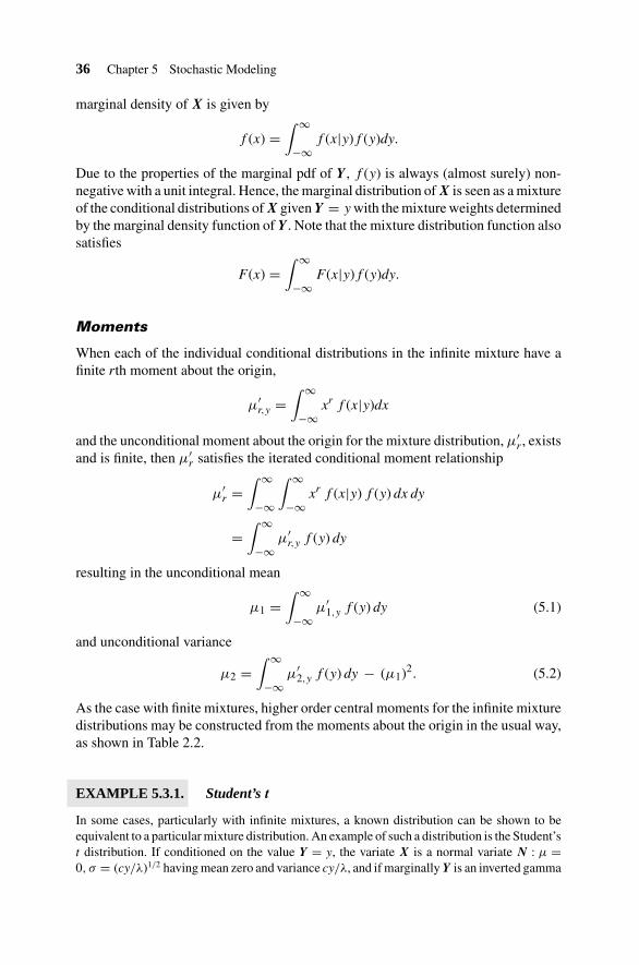
marginal density of X is given by
f (x) =∫ ∞
−∞f (x|y)f (y)dy.
Due to the properties of the marginal pdf of Y , f (y) is always (almost surely) non-negative with a unit integral. Hence, the marginal distribution of X is seen as a mixtureof the conditional distributions of X given Y = y with the mixture weights determinedby the marginal density function of Y . Note that the mixture distribution function alsosatisfies
F (x) =∫ ∞
−∞F (x|y)f (y)dy.
Moments
When each of the individual conditional distributions in the infinite mixture have afinite rth moment about the origin,
μ′r,y =
∫ ∞
−∞xr f (x|y)dx
and the unconditional moment about the origin for the mixture distribution, μ′r, exists
and is finite, then μ′r satisfies the iterated conditional moment relationship
μ′r =
∫ ∞
−∞
∫ ∞
−∞xr f (x|y) f (y) dx dy
=∫ ∞
−∞μ′
r,y f (y) dy
resulting in the unconditional mean
μ1 =∫ ∞
−∞μ′
1,y f (y) dy (5.1)
and unconditional variance
μ2 =∫ ∞
−∞μ′
2,y f (y) dy − (μ1)2. (5.2)
As the case with finite mixtures, higher order central moments for the infinite mixturedistributions may be constructed from the moments about the origin in the usual way,as shown in Table 2.2.
EXAMPLE 5.3.1. Student’s t
In some cases, particularly with infinite mixtures, a known distribution can be shown to beequivalent to a particular mixture distribution. An example of such a distribution is the Student’st distribution. If conditioned on the value Y = y, the variate X is a normal variate N : μ =0, σ = (cy/λ)1/2 having mean zero and variance cy/λ, and if marginally Y is an inverted gamma

5.3 Mixture Distributions 37
variate Y ∼ 1/(γ : λ = 1/b, c) having mean λ/(c − 1) and variance λ2/(c − 1)2(c − 2) thenthe marginal distribution of X alone is that of t : ν = 2c. To prove this, note from Chapter 33the pdf of the normal variate X ∼ N : o, (cy/λ)1/2 is
f (x|y) = λ1/2
(2πcy)1/2exp
(−λx2
2cy
)
and from Chapter 22 the pdf of the inverted gamma variate Y ∼ 1/γ : 1/b, c is
f (y) =exp
(− λ
y
)λc
yc+1�(c)
and hence the marginal pdf of X is found to be that of a t : ν = 2c variate, since
f (x) =∫ ∞
0
f (x|y)f (y) dy
=∫ ∞
0
λc+ 12
(2πc)12 yc+ 3
2 �(c)exp
(−λ
y
[1 + x2
2c
])dy
= λc+ 12 �
(c + 1
2
)(2πc)
12 �(c)
(λ
[1 + x2
2c
])c+ 12
×∫ ∞
0
exp(− λ
y
[1 + x2
2c
])(λ
[1 + x2
2c
])c+ 32
yc+ 32 �
(c + 1
2
) dy
= �(
(ν+1)2
)(νπ)
12 �
(ν
2
) [1 + x2
ν
] (ν+1)2
where ν = 2c. See Chapter 43.
Moments
Note that the mean of a Student’s t variate, t : 2c indeed satisfies the relation inEquation (5.1), with unconditional mean μ1 = 0 since μ′
1,y = 0, and the variancesatisfies the relation in Equation (5.2), since μ′
2,y = c y/λ and hence
μ2 =∫ ∞
0
c y
λf (y) dy − 0
= c
λ
∫ ∞
0y
exp(−λ
y
)λc
yc+1�(c)dy
= c
λ
[λ
c − 1
]= c
c − 1.
Simulation
Simulation of a variate from an infinite mixture distribution is undertaken in twosteps. First the variate Y is drawn from its marginal distribution F (y). Then, given
38 Chapter 5 Stochastic Modeling
this drawn value of Y = yY the variate X is drawn from its conditional distribution.The draw of Y = yY is then discarded.
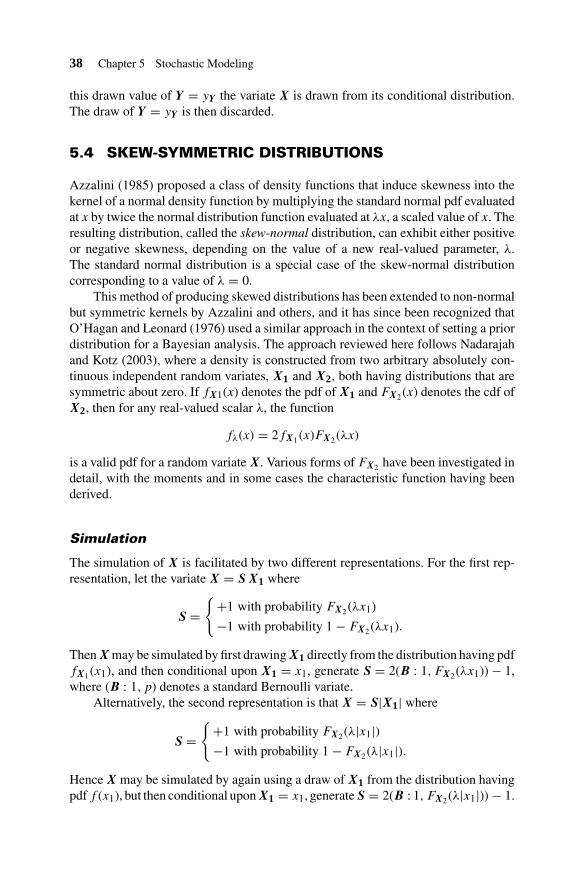
5.4 SKEW-SYMMETRIC DISTRIBUTIONS
Azzalini (1985) proposed a class of density functions that induce skewness into thekernel of a normal density function by multiplying the standard normal pdf evaluatedat x by twice the normal distribution function evaluated at λx, a scaled value of x. Theresulting distribution, called the skew-normal distribution, can exhibit either positiveor negative skewness, depending on the value of a new real-valued parameter, λ.The standard normal distribution is a special case of the skew-normal distributioncorresponding to a value of λ = 0.
This method of producing skewed distributions has been extended to non-normalbut symmetric kernels by Azzalini and others, and it has since been recognized thatO’Hagan and Leonard (1976) used a similar approach in the context of setting a priordistribution for a Bayesian analysis. The approach reviewed here follows Nadarajahand Kotz (2003), where a density is constructed from two arbitrary absolutely con-tinuous independent random variates, X1 and X2, both having distributions that aresymmetric about zero. If fX1(x) denotes the pdf of X1 and FX2 (x) denotes the cdf ofX2, then for any real-valued scalar λ, the function
fλ(x) = 2fX1 (x)FX2 (λx)
is a valid pdf for a random variate X. Various forms of FX2 have been investigated indetail, with the moments and in some cases the characteristic function having beenderived.
Simulation
The simulation of X is facilitated by two different representations. For the first rep-resentation, let the variate X = S X1 where
S ={
+1 with probability FX2 (λx1)
−1 with probability 1 − FX2 (λx1).
Then X may be simulated by first drawing X1 directly from the distribution having pdffX1 (x1), and then conditional upon X1 = x1, generate S = 2(B : 1, FX2 (λx1)) − 1,where (B : 1, p) denotes a standard Bernoulli variate.
Alternatively, the second representation is that X = S|X1| where
S ={
+1 with probability FX2 (λ|x1|)−1 with probability 1 − FX2 (λ|x1|).
Hence X may be simulated by again using a draw of X1 from the distribution havingpdf f (x1), but then conditional upon X1 = x1, generate S = 2(B : 1, FX2 (λ|x1|)) − 1.

5.5 Distributions Characterized by Conditional Skewness 39
Quantile x
Prob
abili
ty d
ensi
ty
−3 −2 −1 3210
0.2
0.4
0.6
0.8
λ = 0
λ = −0.75
λ = 50
λ = 1
.5
λ = −5
Figure 5.3. Probability density function for the skew-normal variate SN : λ.
EXAMPLE 5.4.1. Skew-Normal
Azzalini’s (1985) initial class of distributions take both X1 and X2 to be N : 0, 1 variates.Then
fλ(x) = 2exp(−x2/2)
(2π)1/2
∫ x
−∞
exp(−(λ u)2/2)
(2π)1/2du (5.3)
Figure 5.3 displays the pdf of the skew-normal X for a selection of λ values, while Figure 5.4displays the corresponding cdfs. Note when λ = 0 the distribution reverts to that of a N : 0, 1variate, but with λ < 0 the skew-normal distribution is negatively skewed and when λ > 0 thedistribution is positively skewed.
The skew-normal distribution for fixed λ is unimodal, in particular with the natural loga-rithm of the pdf fλ(x) in Equation (5.3) being a concave function of x. In addition, as λ → ∞,the distribution of the variate X tends to the half-normal distribution.
5.5 DISTRIBUTIONS CHARACTERIZED BY CONDITIONALSKEWNESS
Fernandez and Steel (1998) suggest an alternative way to modify a symmetric den-sity such that the result is a skewed density. Their approach relies upon taking aunivariate symmetric about zero and unimodal density function f (x) and a positivereal-valued scalar, γ . They then define the new density function conditional on the

40 Chapter 5 Stochastic Modeling
Quantile x−3 −2 −1 3210
0.5
1.0
Probabilityα λ
= 0
λ = −
0.75
λ = 50
λ =
1.5
λ = −5
Figure 5.4. Distribution function for the skew-normal variate SN : λ.
scalar variable
f (x|γ) = 2
γ + 1γ
{f
(x
γ
)I[0,∞)(x) + f (γx) I(−∞,0)(x)
}.
Here the parameter γ > 0 introduces skewness into the symmetric f by scaling overthe entire range of x, albeit with differing impact for x > 0 than for x ≤ 0. Underthis framework, although the density retains its single mode at x = 0, the distributionremains symmetric only when γ = 1, with positive skewness associated for γ > 1and negative skewness associated with γ < 1. The pdf for the conditional skewnessmodel is shown for γ equal to 0.5, 1, and 4 in Figure 5.5, whereas the correspondingdistribution functions are shown in Figure 5.6.
An advantage of the approach is that it leads to closed form solutions for themoments of the constructed skewed distributions in terms of the moments of the un-derlying symmetric distribution. In addition, the pdf of the skewed distribution retainsthe differentiability properties of the original pdf from the underlying distribution. Theconditioning framework is especially appealing in a Bayesian setting, where modelsare typically constructed using composition.
Moments
Given a value of γ , the rth moment about the origin, μ′r,γ satisfies
μ′r,γ = μ′
r
γr+1 + (−1)r
γr+1
γ + 1γ
(5.4)

5.5 Distributions Characterized by Conditional Skewness 41
Quantile x
Prob
abili
ty d
ensi
ty
−6 −4 −2 0 642 108
0.1
0.2
0.3
0.4
γ = 4
γ = 0.5
γ = 1
Figure 5.5. Probability function for the conditional skewness model of Fernandez and Steel (1998).
Quantile x−6 −4 −2 0 642 108
0.5
1.0
Probabilityα
γ = 4
γ = 0.5
γ = 1
Figure 5.6. Distribution function for the conditional skewness model of Fernandez and Steel (1998).
where μ′r denotes the rth moment about the origin for the underlying symmetric
distribution having pdf f . Note that the rth moment about the origin is real-valuedonly for integer-valued r.

42 Chapter 5 Stochastic Modeling
From Equation (5.4) we have
μ1,γ = μ′1
γ2 − 1γ2
γ + 1γ
= μ′1γ4 − 1
γ3 + γ
and
μ2,γ = μ′2
γ6 + 1
γ4 + γ2 − μ21,γ .
Higher order central moments may be constructed from the moments about the originin the usual way shown in Table 2.2. In particular, the coefficient of skewness, η3 =μ3/μ
3/22 , is
η3 =(
γ − 1
γ
) (μ′
3 + 2μ′ 31 − 3μ′
1μ′2
) (γ2 + 1
γ2
)+ 3μ′
1μ′2 − 4μ′ 3
1{(μ′
2 − μ′ 21
) (γ2 + 1
γ2
)+ 2μ′ 2
1 − μ′2
}3/2 .
Due to the relative similarity of γ and 1/γ in Equation (5.4), it can be shownthat when r is even, the rth moment about the origin under a value γ is identical tothe rth moment about the origin under a value 1/γ . However, when r is odd, theabsolute value of the rth moment about the origin under a value γ is the same asthe absolute value of the rth moment about the origin under a value 1/γ , but one willbe positive and the other will be negative.
5.6 DEPENDENT VARIATES
When observations are not independent, even when each of the individual variatesXi, i = 1, 2, . . . , n have common marginal distribution F , the empirical distributionfunction FE(x) need not directly reflect the form of this marginal distribution. Hence,a single univariate distribution is in general not sufficient to describe the propertiesof the multivariate X = (X1, X2, . . . , Xn). Instead, we tend to think about bringingindependent variates into regression-type models that describe the relationship of thevariates, one to another.
When modeling dependent variates, it is often useful to think about describingthe joint density of the multivariate using conditioning. By identifying conditioningvariates, one can sometimes build up from specific univariate distributions to thedesired multivariate distribution via conditioning relationships. The specification ofthe conditioning relationships is therefore considered part of the modeling process.Many general classes of models have been developed using this approach. However,it is beyond the scope of this book to explore any but the simplest of model structures.Hence, to illustrate how to use statistical distributions within the context of modelingdependent data, we demonstrate the ideas through a relatively simple example.

5.6 Dependent Variates 43
EXAMPLE 5.6.1. Autoregressive Order One Model
Consider the multivariate X = (X1, X2, . . . , Xn) and assume that there exists a natural orderingof the variates according to t = 1, 2, . . . , n. The conditioning relationship given by
xt = φ xt−1 + εt, where the error variate εt ∼ N : 0, 1 (5.5)
means that conditional upon Xt−1 = xt−1 (and φ) the variate Xt ∼ N : φ xt−1, 1. The model inEquation (5.5) is generally referred to as an autoregressive order one (AR(1)) model.
When observations exhibit first-order serial correlation, it means that the samplecorrelation between consecutively observed variates is non-negligible. That is, thereis a pattern in the observed data that indicates a structure exists beyond what wouldbe consistent with independent variates. However, this pattern may indeed be veryuseful if the prediction of future realized variates is a modeling objective.
To construct the joint distribution of the data, based on the assumption that theerror variates εt , for t = 1, 2, . . . , n are i.i.d N : 0, 1, we use the conditioning re-lationship implied by Equation (5.5) and the principle of composition discussed inSection 4.4. The joint density for the multivariate X = (X1, X2, . . . , Xn) can be de-scribed as the product of a marginal density and n − 1 successive conditional densities
f (x) = f (x1)f (x2|x1)f (x3|x2, x1) · · · f (xn|xn−1, xn−2, . . . , x1). (5.6)
In this particular example and due to the AR(1) model structure, for t ≥ 2, thedensities in Equation (5.6) have the same form
f (xt|xt−1, xt−2, . . . , x1) = f (xt|xt−1)
= fεt (xt − φ xt−1)
= 1
(2 π)1/2 exp
(−(xt − φ xt−1)2
2
).
The first term in Equation (5.6) is problematic for |φ| ≥ 1, however, for |φ| < 1 thevariate X1 ∼ N : 0, (1 − φ2)−1. The joint density of the multivariate is then
f (x) =(1 − φ2
)1/2
(2 π)1/2 exp
(−(
1 − φ2)(
x21
)2
)n∏
t=2
1
(2 π)1/2 exp
(−(xt − φ xt−1)2
2
)
=(1 − φ2
)1/2
(2 π)n/2 exp
(−1
2
[(1 − φ2)
(x2
1
) +n∑
t=2
(xt − φ xt−1)2
]).
Chapter 38 details many results from dependent structures generated by queues.Readers interested in more complex time series dependency structures are directed toBox, Jenkins, and Reinsel (2008).

Chapter 6
Parameter Inference
6.1 INTRODUCTION
In this chapter we review common methods of inference, namely the Method of Per-centiles (MP), the Method of Moments (MM), Maximum Likelihood (ML) inference,and Bayesian (B) inference. Here we focus only on parameter inference and, wherepossible, point and interval estimation. Inferential frameworks apply to both contin-uous and discrete variates and so here we refer here to both a probability densityfunction for the continuous variate and the probability function for a discrete variateas simply a probability function. As before, integrals are used to denote either inte-gration or summation, depending on whether the relevant argument has continuousor discrete support.
The purpose of this chapter is to summarize the basic ideas behind each inferentialmethod and to facilitate the use of the distributions provided in the latter portion of thisbook. Many more pages could have been devoted to each of the methods summarizedhere, but instead more detailed discussions already available are recommended forfurther reading. In addition, the book by Cox (2006) provides a lucid overview of thefundamental principles of statistical inference from a relatively pragmatic point ofview.
6.2 METHOD OF PERCENTILES ESTIMATION
The idea behind the method of percentiles is simply to match the quantiles of theempirical distribution function, FE(x), to the theoretical quantile xX implied by aparticular distribution function Fθ(x). Here the subscript θ emphasizes that the dis-tribution function (previously denoted by FX(x) or simply F (x)) depends upon thevalue of the potentially vector valued parameter θ.
Consider the case where observations are i.i.d. but with ordered realized variatesx1 ≤ x2 ≤ · · · ≤ xn. Then xi denotes the (i/n)th empirical quantile, or equiva-lently, the 100(i/n)th percentile. In the scalar case, the method of percentiles finds a
Statistical Distributions, Fourth Edition, by Catherine Forbes, Merran Evans, Nicholas Hastings,and Brian PeacockCopyright © 2011 John Wiley & Sons, Inc.
44

6.3 Method of Moments Estimation 45
parameter value θMP for a selected distribution Fθ(x) such that when F is evaluatedat the empirical quantile xi, its value is equal to i/n. That is, F
θMP(xi) = 1/n. This
is equivalent to finding θMP such that the corresponding inverse distribution functionsatisfies G
θMP(i/n) = xi.
EXAMPLE 6.2.1. Exponential Distribution
In this example θ is the scale parameter b. (See Chapter 17.) To find θMP = b for the E : b wefirst note that
Fb(x) = 1 − exp(−x/b)
Gb(α) = −b log(1 − α).
Using the inverse distribution function associated with the probability i/n, we find b such that
Gb(i/n) = xi,
resulting in
b = xi log(
n
n − i
).
Note that in this case the method may be applied to any of the empirical quantiles, except forthe last associated with xn.
The approach is relatively easy to implement, even if analytical expression for the inversefunction G is not available. When the specified distribution involves more than one parameter,solving a set of equations based on more than one empirical quantile will produce the parameterestimates. Note the approach is easily adapted to the case of censoring; see Chapter 14.
Despite its intuitive appeal, the method of percentiles approach does not necessarily pro-duce estimators with good statistical properties. It may, however, provide a suitable startingvalue for other iterative estimation methods.
6.3 METHOD OF MOMENTS ESTIMATION
Method of moments estimation seeks to find parameter values that set theoreti-cal (population) moments equal to the corresponding sample moments. Supposethe distribution of interest depends upon a k-dimensional parameter vector, θ, andthat the first k moments about the origin of the distribution, μ′
r, for r = 1, 2, . . . , k,exist and are finite. To emphasize that theoretically these moments depend upon θ,here we denote the rth moment as μ′
r(θ). Let m′r = 1
n
∑ni=1 xr
i denote the rthsample moment about the origin. A method of moments estimator θMM is simplya value of θ simultaneously satisfying each of the k equations
μ′r(θMM) = m′
r, for r = 1, 2, . . . k. (6.1)
Note that Equation (6.1) is not the only set of moment equations that produce methodof moments estimator. For example, let mr denote the rth (unbiased) sample moment
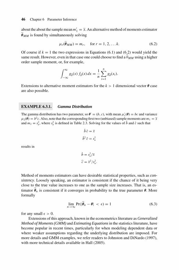
46 Chapter 6 Parameter Inference
about the about the sample mean m′1 = x. An alternative method of moments estimator
θMM is found by simultaneously solving
μr(θMM) = mr, for r = 1, 2, . . . k. (6.2)
Of course if k = 1 the two expressions in Equations (6.1) and (6.2) would yield thesame result. However, even in that case one could choose to find a θMM using a higherorder sample moment, or, for example,
∫ ∞
−∞gθ(x) fθ(x) dx = 1
n
n∑i=1
gθ(xi).
Extensions to alternative moment estimators for the k > 1 dimensional vector θ caseare also possible.
EXAMPLE 6.3.1. Gamma Distribution
The gamma distribution has two parameter, so θ′ = (b, c), with mean μ′1(θ) = bc and variance
μ2(θ) = b2c. Also, note that the corresponding first two (unbiased) sample moments are m1 = x
and m2 = s2u, where s2
u is defined in Table 2.3. Solving for the values of b and c such that
b c = x
b2 c = s2u
results in
b = s2u/x
c = x2/s2u.
Method of moments estimators can have desirable statistical properties, such as con-sistency. Loosely speaking, an estimator is consistent if the chance of it being veryclose to the true value increases to one as the sample size increases. That is, an es-timator θn is consistent if it converges in probability to the true parameter θ. Moreformally
limn→∞ Pr(|θn − θ| < ε) = 1 (6.3)
for any small ε > 0.Extensions of this approach, known in the econometrics literature as Generalized
Method of Moments (GMM) and Estimating Equations in the statistics literature, havebecome popular in recent times, particularly for when modeling dependent data orwhere weaker assumptions regarding the underlying distribution are imposed. Formore details and GMM examples, we refer readers to Johnston and DiNardo (1997),with more technical details available in Hall (2005).

6.4 Maximum Likelihood Inference 47
6.4 MAXIMUM LIKELIHOOD INFERENCE
When the joint density for a set of variates is viewed as a function of the parametersalone, rather than as a function of the variates themselves, that function is called alikelihood function. Hence the likelihood function, L(θ), is defined as
L(θ) = fθ(x)
and in particular when variates are i.i.d.
L(θ) =n∏
i=1
fθ(xi).
Here log fθ(x) is a scalar function of a k-dimensional variable θ and as in Chapter 5x = (x1, x2, . . . , xn). A value of the parameter θ that maximizes L (θ) is called amaximum likelihood estimator (MLE), and is denoted by θML. It is often easier tomaximize the log-likelihood function, log L(θ), and since the (natural) logarithmicfunction is monotonically increasing in θ, the same value of θML maximizes bothL (θ) and log L(θ).
Properties of MLEs
Under quite general conditions, MLEs have a number of favorable properties. Weconsider here those associated with i.i.d. variates, although generalizations of theseproperties hold for a likelihood function based on dependent variates in many settings.These properties essentially all have to do with the behavior of MLEs when the samplesize is very large. We place an additional subscript ‘n’ on θML to emphasize the factthat any particular MLE will be a function of the sample size, n.
Consistency. Under mild conditions, MLEs converge to the true parameter valueas the sample size increases. See Equation (6.3).
Asymptotic Normality. As the sample size increases, the distribution of theMLE approaches that of a (potentially) Multivariate Normal variate. In par-ticular,
√n
(θML,n − θ
)Dist→ MN : 0, i (θ)−1 .
Here 0 denotes the k-dimensional zero vector. The (k × k) dimensional matrixi (θ) is called the (Fisher) information, and is equal to minus the expectedsecond partial derivative matrix of the log-probability function of a singlevariate, evaluated at the “true” parameter, θ
i (θ) = −E
[∂2 log fθ (x)
∂θ∂θ′
]= −
∫ ∞
−∞
[∂2 log f (x|θ)
∂θ∂θ′
]fθ (x) dx. (6.4)
In the multidimensional setting, ∂ log fθ (x)/∂θ denotes a column vector ofpartial derivatives with ∂ log fθ (x)/∂θr in the rth row, θr denotes the rth

48 Chapter 6 Parameter Inference
component of θ, and ∂2 log f (x|θ)/∂θ∂θ′ denotes the matrix of second orderpartial derivatives with row (r) and column (c) element ∂2 log fθ (x)/∂θr∂θc.
Asymptotic Efficiency. MLEs are asymptotically efficient, meaning that evenif an alternative estimator, θn, is available, with
√n
(θn − θ
)Dist→ MN : 0, δ,
then always δ ≥ i (θ)−1 . HereDist→ denotes convergence in distribution, mean-
ing that as the sample size increases then the distribution of the (appro-priately scaled and shifted) parameter estimator θn behaves as a MN : 0, δ
variate.
Invariance. Under mild conditions, the MLE of a differentiable function g(θ),is equal to that function evaluated at the MLE of θ. That is, if θML is the MLE
of θ, then g(θML
)is the MLE of g (θ), and further
√n
(g
(θML,n
)− g (θ)
)Dist→ MN : 0,
[∂g (θ)
∂θ
]i (θ)−1
[∂g (θ)
∂θ
]′.
Since g (θ) may be a g ≤ k dimensional vector function of a k-dimensionalvector argument, then
[∂g (θ)/∂θ
]represents the matrix of partial derivatives
with [r, c] element[∂gr (θ)/∂θc
], where gr (θ) denotes the rth scalar function
element of g (θ).[∂g (θ)/∂θ
]′ denotes the transpose of[∂g (θ)/∂θ
].
Approximate Sampling Distribution for Fixed n
To make use of the asymptotic normality result and its associated properties, theinformation matrix i(θ) will commonly need to be estimated and this will usuallybe done in two ways. The first involves using the sample average of second partialderivative matrix of the log-probability function of each variate, evaluated at the MLE
i1 = − 1
n
n∑i=1
∂2 log f (xi|θ)
∂θ∂θ′
∣∣∣∣∣θ=θML
.
The second involves the sample average of the outer product of the first derivative ofthe log-probability function of each variate, evaluated at the MLE
i2 = 1
n
n∑i=1
(∂ log f (xi|θ)
∂θ
) (∂ log f (xi|θ)
∂θ
)′∣∣∣∣∣θ=θML
.
In either case, the resulting approximation for the sampling distribution for the MLE is
θMLapprox∼ MN : θ,
(n−1i
−1)
. A corresponding approximate sampling distribution

6.4 Maximum Likelihood Inference 49
for g(θML
)is
g(θML
)approx∼ MN : g (θ) , n−1
⎡⎣∂g
(θML
)∂θ
⎤⎦ i
−1
⎡⎣∂g
(θML
)∂θ
⎤⎦
′
,
where ∂g(θML
)/∂θ denotes ∂g (θ) /∂θ evaluated at θML.
EXAMPLE 6.4.1. Exponential Sample
Assume X1, X2, . . . , Xn are i.i.d.∼ E : b. Then the log-likelihood function is
log L (b) = log
[n∏
i=1
1
bexp (−xi/b)
]= −n log b − nx/b.
Differentiating the log-likelihood (with respect to b) yields
d log L (b)
db= −nb−1 + nxb−2.
The MLE is found by setting this first derivative to zero, that is,
−nb−1ML + nxb−2
ML = 0
and solving for bML = x. Since x > 0, the second derivative of log L (b) evaluated at bML =−n(x)−2 is negative, confirming that bML maximizes the likelihood function.
Since b is a scalar parameter, the information is a scalar function of b and is found bytwice differentiating log fb(x) = − log b − x/b. In this case,
i (b) = −E
[d2 log f (x|b)
db2
]= b−2
yielding the result (for fixed n) that
xapprox∼ N : b, b2/n.
An approximate 100 (1 − α)% confidence interval for b is given by
x ± zα/2x/√
n
where zd/2 = GN:0,1(1 − α/2) denotes the (1 − α/2)100% quantile of the N : 0, 1 distribution.
The above example is simple enough to permit analytical calculation of the MLEand its associated information. However, in many applications the MLE and theinformation matrix must be computed numerically on a computer. For more detailson the application of maximum likelihood in practice, or for more background on thetheoretical properties involved, see Casella and Berger (2002).

50 Chapter 6 Parameter Inference
6.5 BAYESIAN INFERENCE
For Bayesian analysis of statistical problems, probability statements are considereda measure of belief. Bayesian statistics involves the formal updating of prior (pre-data) beliefs about parameter values in light of observed information (data) through aformal revision of probabilities undertaken using Bayes’ theorem. (See Section 4.5.) Inaddition to one’s subjective view, it is common to summarize prior belief arising froma range of sources, including thought experiments, knowledge of previous analysisof similar data, and consensus opinion.
In this context parameters are treated as though they are random variates with priorbelief regarding parameter values summarized in a prior probability function f (θ).This prior probability function is then revised in light of the likelihood function viaBayes theorem to produce an updated probability function for θ, called the posteriorprobability function
f (θ|x) = f (θ) L (θ)
m (x). (6.5)
The function m (x) in the denominator of Equation (6.5) denotes the so-calledmarginal likelihood, with
m (x) =∫
f (θ) L (θ) dθ. (6.6)
The value of m (x) is found by evaluating the marginal probability function of X
in Equation (6.6) at the observed X = x. Since it is not a function of θ and x isknown, m(x) is constant. As before L (θ) represents the joint probability function ofthe observed data viewed as a function of the unknown parameter, θ. To emphasizethat the distribution of the multivariate X is known conditionally upon a fixed value ofthe parameter θ, the probability function fθ(x) is represented using the conditioningnotation f (x|θ).
The posterior probability function provides the mechanism for computing prob-abilities associated with the posterior distribution. Hence the posterior distributionitself is the complete summary for the unknown parameter. Once obtained, the ex-pected value (when it exists)
θB =∫ ∞
−∞θ f (θ|x) dθ
and the mode of the posterior
θB = maxθ
f (θ|x)
are frequently cited as a representative value from this distribution and are sometimesregarded as point estimators for θ.

6.5 Bayesian Inference 51
Marginal Posteriors
When θ is multivariate, the distribution of the rth element of the parameter vector, θr,may be summarized using its marginal posterior distribution, found in the usual wayby integrating over the remaining parameter components
f (θr|x) =∫
f (θ|x) dθ(r)
where θ(r) denotes all of the elements of θ except the rth element, θr.
EXAMPLE 6.5.1. Exponential Variates with a Gamma Prior
Consider i.i.d. univariates X1, X2, . . . , Xn ∼ E : λ with prior distribution λ ∼ γ : b, c. Thatis, the prior distribution of the parameter λ is that of a Gamma variate with mean bc, having aprior mode of b(c − 1), and with prior probability function for λ > 0 given by
f (λ) = λc−1
bc � (c)exp
{−λ
b
}.
The likelihood function for λ associated with the multivariate X is
L (λ) =n∏
i=1
λ exp {−λxi} = λn exp {−λnx}
so that the posterior probability function has the form
f (λ|x) = λn exp {−λnx} λc−1
bc� (c)exp
{−λ
b
}/m(x)
= λn+c−1
bc� (c)exp
{−λ
[nx + 1
b
]}/m(x).
Since
m (x) =∫ ∞
0
λn+c−1
bc� (c)exp
{−λ
[nx + 1
b
]}dλ
= � (n + c)
bc� (c)[nx + 1
b
]n+c
×∫ ∞
0
[nx + 1
b
]n+c
� (n + c)λn+c−1 exp
{−λ
[nx + 1
b
]}dλ
= bn � (n + c)
� (c) [bnx + 1]n+c
the posterior probability function is
f (λ|x) =[
bnx + 1
b
]n+c1
� (n + c)λn+c−1 exp
{−λ
[nx + 1
b
]}, (6.7)

52 Chapter 6 Parameter Inference
implying
λ|x = γ : b[bnx + 1]−1, (n + c).
Therefore the posterior distribution has a single mode at
λB = b(n + c − 1)/(bnx + 1)
and its mean is
λB = b(n + c)/(bnx + 1).
The shortest available 100 (1 − α)% credibility interval (Lλ, Uλ) would be found such that
0.95 = Pr(Lλ < λ ≤ Uλ|X)
=∫ Uλ
Lλ
f (λ|x) dλ
where f (λ|x) is shown in Equation (6.7).
Often the most difficult part of a Bayesian analysis is computing the marginal like-lihood m(x). However, in recent years the vast improvements in computing capacityand the development of simulation methods have meant that once intractable prob-lems may now be numerically solved. In particular, empirical analyses using Bayesianmethods frequently use so-called Markov chain Monte Carlo (MCMC) methods todraw a sample of parameter values θ from its posterior distribution and to producepoint and interval summaries of that posterior distribution. For a detailed expositionincluding both philosophical and methodological developments, see Robert (2007).
In small dimensional and regular problems, as the sample size increases thereis often little difference between the MLE and Bayesian point estimators. However,in problems with a large set of unknown parameters, the two methods can differsignificantly even for relatively large samples.

Chapter 7
Bernoulli Distribution
A Bernoulli trial is a probabilistic experiment that can have one of two outcomes,success (x = 1) or failure (x = 0), and in which the probability of success is p. Werefer to p as the Bernoulli probability parameter.
An example of a Bernoulli trial is the inspection of a random item from a pro-duction line with the possible result that the item could be acceptable or faulty. TheBernoulli trial is a basic building block for other discrete distributions such as thebinomial, Pascal, geometric, and negative binomial.
Variate B: 1, p.
(The general binomial variate is B: n, p, involving n trials.)
Range x ∈ {0, 1}.Parameter p, the Bernoulli probability parameter, 0 < p < 1.
Distribution function F (0) = 1 − p; F (1) = 1
Probability function f (0) = 1 − p; f (1) = p
Characteristic function 1 + p[exp(it) − 1]
rth Moment about the origin p
Mean p
Variance p(1 − p)
7.1 RANDOM NUMBER GENERATION
R is a unit rectangular variate and B: 1, p is a Bernoulli variate. R ≤ p implies B:1, p takes value 1;R > p implies B: 1, p takes value 0.
7.2 CURTAILED BERNOULLI TRIAL SEQUENCES
The binomial, geometric, Pascal, and negative binomial variates are based on se-quences of independent Bernoulli trials, which are curtailed in various ways, forexample, after n trials or x successes. We shall use the following terminology:
Statistical Distributions, Fourth Edition, by Catherine Forbes, Merran Evans, Nicholas Hastings,and Brian PeacockCopyright © 2011 John Wiley & Sons, Inc.
53

54 Chapter 7 Bernoulli Distribution
p Bernoulli probability parameter (probability of success at a single trial)n Number of trialsx Number of successesy Number of failuresB: n, p Binomial variate, number of successes in n trialsG: p Geometric variate, number of failures before the first successNB: x, p Negative binomial variate, number of failures before the xth success
A Pascal variate is the integer version of the negative binomial variate. Alternativeforms of the geometric and Pascal variates include the number of trials up to andincluding the xth success. These variates are interrelated in various ways, specifiedunder the relevant chapter headings.
7.3 URN SAMPLING SCHEME
The selection of items from an urn, with a finite population N of which Np are ofthe desired type or attribute and N(1 − p) are not, is the basis of the Polya family ofdistributions.
A Bernoulli variate corresponds to selecting one item (n = 1) with probabilityp of success in choosing the desired type. For a sample consisting of n independentselections of items, with replacement, the binomial variate B: n, p is the number x
of desired items chosen or successes, and the negative binomial variate NB: x, p isthe number of failures before the xth success. As the number of trials or selections n
tends to infinity, p tends to zero, and np tends to a constant λ, the binomial variatetends to the Poisson variate P: λ with parameter λ = np.
If sample selection is without replacement, successive selections are not inde-pendent, and the number of successes x in n trials is a hypergeometric variate H: N,x, n. If two items of the type corresponding to that selected are replaced each time,thus introducing “contagion,” the number of successes x in n trials is then a negativehypergeometric variate, with parameters N, x, and n.
7.4 NOTE
The following properties can be used as a guide in choosing between the binomial,negative binomial, and Poisson distribution models:
Binomial Variance < meanNegative binomial Variance > meanPoisson Variance = mean

Chapter 8
Beta Distribution
Applications include modeling random variables that have a finite range, a to b. Anexample is the distribution of activity times in project networks. The beta distributionis frequently used as a prior distribution for binomial proportions in Bayesian analysis.
Variate β : ν, ω.
Range 0 ≤ x ≤ 1.
Shape parameters ν > 0, ω > 0.
This beta distribution (of the first kind) is U shaped if ν < 1, ω < 1 and J
shaped if (ν − 1)(ω − 1) < 0, and is otherwise unimodal.
Distribution function Often called the incomplete beta function. (SeePearson, 1968.)
Probability density func-tion
xν−1(1 − x)ω−1/B(ν, ω), where B(ν, ω) is thebeta function with arguments ν, ω, given by
B(ν, ω) = ∫ 10 uν−1(1 − u)ω−1du
rth Moment about the
origin∏r−1
i=0(ν + i)
(ν + ω + i)= B(ν + r, ω)
B(ν, ω)
Mean ν/(ν + ω)
Variance νω/[(ν + ω)2(ν + ω + 1)
]Mode (ν − 1)/(ν + ω − 2), ν > 1, ω > 1
Coefficient of
skewness2(ω − ν)(ν + ω + 1)1/2
(ν + ω + 2)(νω)1/2
Statistical Distributions, Fourth Edition, by Catherine Forbes, Merran Evans, Nicholas Hastings,and Brian PeacockCopyright © 2011 John Wiley & Sons, Inc.
55

56 Chapter 8 Beta Distribution
Coefficient ofkurtosis
3(ν + ω)(ν + ω + 1)(ν + 1)(2ω − ν)
νω(ν + ω + 2)(ν + ω + 3)
+3(ν + ω + 1)(ν − ω)
ω(ν + ω + 2)
Coefficient of variation
(ω
ν(ν + ω + 1)
)1/2
Probability density func-tion if ν and ω are integers
(ν + ω − 1)!xν−1(1 − x)ω−1
(ν − 1)!(ω − 1)!
Probability density func-tion if range is a ≤ x ≤ b.Herea is a location param-eter and b − a a scale pa-rameter.
(x − a)ν−1(b − x)ω−1
B(ν, ω)(b − a)ν+ω−1 .
8.1 NOTES ON BETA AND GAMMA FUNCTIONS
The beta function with arguments ν, ω is denoted B(ν, ω); ν, ω > 0. The gammafunction with argument c is denoted �(c); c > 0. The di-gamma function with argu-ment c is denoted ψ(c); c > 0.
Definitions
Beta function:
B(ν, ω) =∫ 1
0uν−1(1 − u)ω−1 du
Gamma function:
�(c) =∫ ∞
0exp(−u)uc−1 du
Di-gamma function:
ψ(c) = d
dc
[log �(c)
] = d�(c)/dc
�(c)
Interrelationships
B(ν, ω) = �(ν)�(ω)
�(ν + ω)= B(ω, ν)
�(c) = (c − 1)�(c − 1)
B(ν + 1, ω) = ν
ν + ωB(ν, ω)
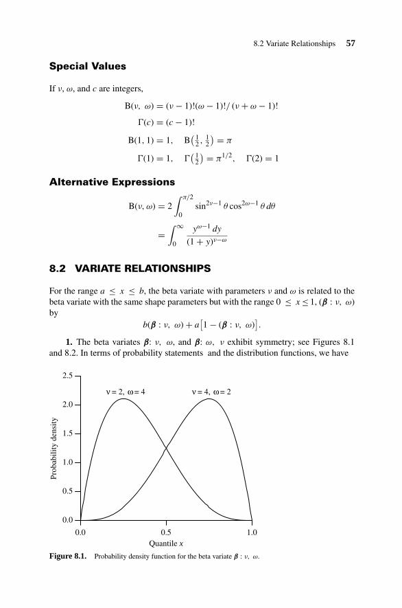
8.2 Variate Relationships 57
Special Values
If ν, ω, and c are integers,
B(ν, ω) = (ν − 1)!(ω − 1)!/ (ν + ω − 1)!
�(c) = (c − 1)!
B(1, 1) = 1, B( 1
2 , 12
) = π
�(1) = 1, �( 1
2
) = π1/2, �(2) = 1
Alternative Expressions
B(ν, ω) = 2∫ π/2
0sin2ν−1 θ cos2ω−1 θ dθ
=∫ ∞
0
yω−1 dy
(1 + y)ν−ω
8.2 VARIATE RELATIONSHIPS
For the range a ≤ x ≤ b, the beta variate with parameters ν and ω is related to thebeta variate with the same shape parameters but with the range 0 ≤ x ≤ 1, (β : ν, ω)by
b(β : ν, ω) + a[1 − (β : ν, ω)
].
1. The beta variates β: ν, ω, and β: ω, ν exhibit symmetry; see Figures 8.1and 8.2. In terms of probability statements and the distribution functions, we have
Quantile x
Prob
abili
ty d
ensi
ty
ν = 2, ω = 4 ν = 4, ω = 2
0.0
0.5
1.0
1.5
2.0
2.5
0.0 0.5 1.0
Figure 8.1. Probability density function for the beta variate β : ν, ω.
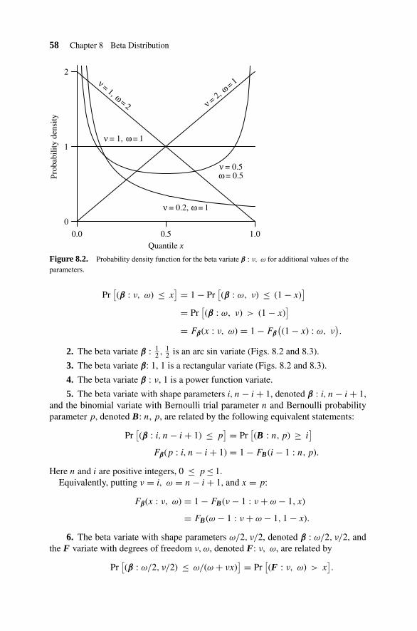
58 Chapter 8 Beta Distribution
Quantile x
Prob
abili
ty d
ensi
ty
ν = 1, ω= 2 ν = 2, ω= 1
ν = 1, ω = 1
ν = 0.5 ω = 0.5
ν = 0.2, ω = 1
0
1
2
0.0 0.5 1.0
Figure 8.2. Probability density function for the beta variate β : ν, ω for additional values of theparameters.
Pr[(β : ν, ω) ≤ x
] = 1 − Pr[(β : ω, ν) ≤ (1 − x)
]= Pr
[(β : ω, ν) > (1 − x)
]= Fβ(x : ν, ω) = 1 − Fβ
((1 − x) : ω, ν
).
2. The beta variate β : 12 , 1
2 is an arc sin variate (Figs. 8.2 and 8.3).
3. The beta variate β: 1, 1 is a rectangular variate (Figs. 8.2 and 8.3).
4. The beta variate β : ν, 1 is a power function variate.
5. The beta variate with shape parameters i, n − i + 1, denoted β : i, n − i + 1,and the binomial variate with Bernoulli trial parameter n and Bernoulli probabilityparameter p, denoted B: n, p, are related by the following equivalent statements:
Pr[(β : i, n − i + 1) ≤ p
] = Pr[(B : n, p) ≥ i
]Fβ(p : i, n − i + 1) = 1 − FB (i − 1 : n, p).
Here n and i are positive integers, 0 ≤ p ≤ 1.Equivalently, putting ν = i, ω = n − i + 1, and x = p:
Fβ(x : ν, ω) = 1 − FB (ν − 1 : ν + ω − 1, x)
= FB (ω − 1 : ν + ω − 1, 1 − x).
6. The beta variate with shape parameters ω/2, ν/2, denoted β : ω/2, ν/2, andthe F variate with degrees of freedom ν, ω, denoted F: ν, ω, are related by
Pr[(β : ω/2, ν/2) ≤ ω/(ω + νx)
] = Pr[(F : ν, ω) > x
].

8.3 Parameter Estimation 59
Quantile x
Prob
abili
ty α
0.0
0.5
1.0
0.0 0.5 1.0
ν = 2
, ω=
4 ν = 1, ω= 1
ν = 0.5, ω= 0.5
Figure 8.3. Distribution function for the beta variate β : ν, ω.
Hence the inverse distribution function Gβ(α : ω/2, ν/2) of the beta variate β :ω/2, ν/2 and the inverse survival function ZF (α : ν, ω) of the F variate F: ν, ω arerelated by
(ω/ν){[
1/Gβ(α : ω/2, ν/2)] − 1
} = ZF (α : ν, ω)
= GF (1 − α : ν, ω)
where α denotes probability.
7. The independent gamma variates with unit scale parameter and shape param-eter ν, denoted γ : 1, ν, and with shape parameter ω, denoted γ : 1, ω, respectively,are related to the beta variate β : ν, ω by
β : ν, ω ∼ (γ : 1, ν)/[(γ : 1, ν) + (γ : 1, ω)
].
8. As ν and ω tend to infinity, such that the ratio ν/ω remains constant, theβ : ν, ω variate tends to the standard normal variate N: 0, 1.
9. The variate β : ν, ω corresponds to the one-dimensional Dirichlet variatewith ν = c1, ω = c0. The Dirichlet distribution is the multivariate generalization ofthe beta distribution.
8.3 PARAMETER ESTIMATION
Parameter Estimator Method
ν x{[
x(1 − x)/s2] − 1
}Matching moments
ω (1 − x){[
x(1 − x)/s2] − 1
}Matching moments

60 Chapter 8 Beta Distribution
The maximum-likelihood estimators ν and ω are the solutions of the simultaneousequations
ψ(ν) − ψ(ν + ω) = n−1n∑
i=1
log xi
ψ(ω) − ψ(ν + ω) = n−1n∑
i=1
log(1 − xi).
8.4 RANDOM NUMBER GENERATION
If ν and ω are integers, then random numbers of the beta variate β : ν, ω can be com-puted from random numbers of the unit rectangular variate R using the relationshipwith the gamma variates γ : 1, ν and γ : 1, ω as follows:
γ : 1, ν ∼ − logν∏
i=1
Ri
γ : 1, ω ∼ − logω∏
j=1
Ri
β : ν, ω ∼ γ : 1, ν
(γ : 1, ν) + (γ : 1, ω).
8.5 INVERTED BETA DISTRIBUTION
The beta variate of the second kind, also known as the inverted beta or beta primevariate with parameters ν and ω, denoted Iβ : ν, ω, is related to the β : ν, ω variateby
Iβ : ν, ω ∼ (β : ν, ω)/[1 − (β : ν, ω)]
and to independent standard gamma variates by
Iβ : ν, ω ∼ (γ : 1, ν)/(γ : 1, ω).
The inverted beta variate with shape parameters ν/2, ω/2 is related to the F : ν, ω
variate by
Iβ : ν/2, ω/2 ∼ (ν/ω)F : ν, ω.
The pdf is xν−1/[B(ν, ω)(1 + x)ν+ω], x > 0.

8.7 Beta Binomial Distribution 61
8.6 NONCENTRAL BETA DISTRIBUTION
The noncentral beta variate β : ν, ω, δ is related to the independent noncentralchi-squared in variate χ2 : ν, δ and the central chi-squared variate χ2 : ω by
χ2 : ν, δ
(χ2 : ν, δ) + (χ2 : ω)∼ β : ν, ω, δ.
8.7 BETA BINOMIAL DISTRIBUTION
If the parameter p of a binomial variate B: n, p is itself a beta variate β : ν, ω, theresulting variate is a beta binomial variate with probability function(
n
x
)B(ν + x, n + ω − x)
B(ν, ω)
with mean nν/(ν + ω) and variance
nνω(n + ν + ω)/[(ν + ω)2(1 + ν + ω)].
This is also called the binomial beta or compound binomial distribution. For integer ν
and ω, this corresponds to the negative hypergeometric distribution. For ν = ω = 1,it corresponds to the discrete rectangular distribution. A multivariate extension of thisis the Dirichlet multinomial distribution.
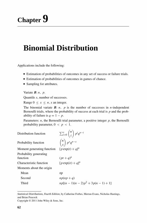
Chapter 9
Binomial Distribution
Applications include the following:
• Estimation of probabilities of outcomes in any set of success or failure trials.
• Estimation of probabilities of outcomes in games of chance.
• Sampling for attributes.
Variate B: n, p.
Quantile x, number of successes.
Range 0 ≤ x ≤ n, x an integer.
The binomial variate B: n, p is the number of successes in n-independentBernoulli trials, where the probability of success at each trial is p and the prob-ability of failure is q = 1 − p.
Parameters: n, the Bernoulli trial parameter, a positive integer p, the Bernoulliprobability parameter, 0 < p < 1.
Distribution function∑x
i=0
(n
i
)piqn−i
Probability function
(n
x
)pxqn−x
Moment generating function [p exp(t) + q]n
Probability generatingfunction (pt + q)n
Characteristic function [p exp(it) + q]n
Moments about the origin
Mean np
Second np(np + q)
Third np[(n − 1)(n − 2)p2 + 3p(n − 1) + 1]
Statistical Distributions, Fourth Edition, by Catherine Forbes, Merran Evans, Nicholas Hastings,and Brian PeacockCopyright © 2011 John Wiley & Sons, Inc.
62
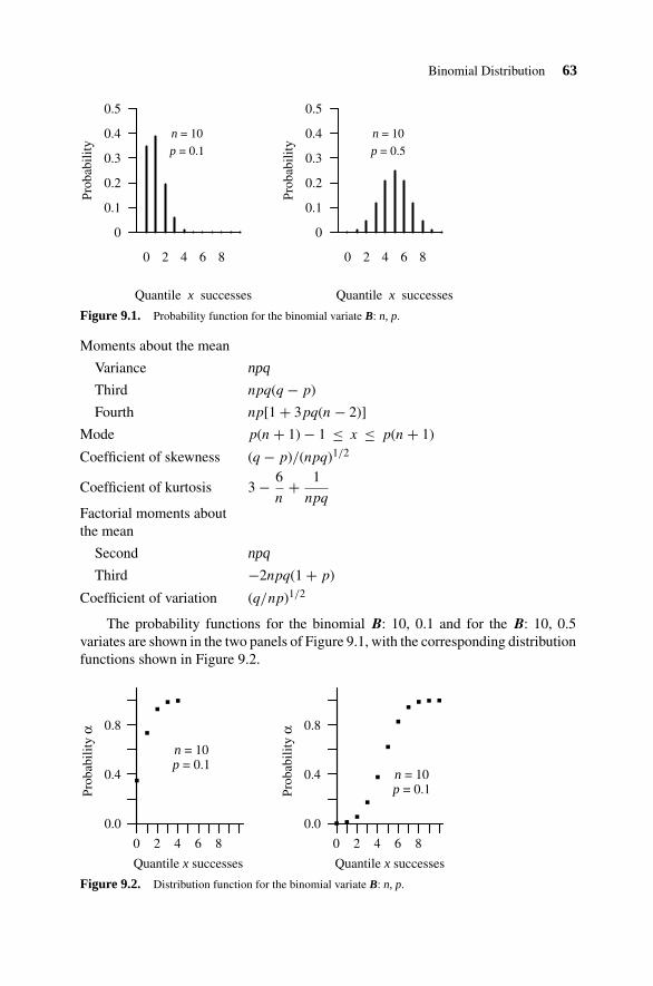
Binomial Distribution 63
Quantile x successes
Prob
abili
ty
0
0.1
0.2
0.3
0.4
0.5
0 2 4 6 8
n = 10
p = 0.1
Quantile x successesPr
obab
ility
0
0.1
0.2
0.3
0.4
0.5
0 2 4 6 8
n = 10
p = 0.5
Figure 9.1. Probability function for the binomial variate B: n, p.
Moments about the mean
Variance npq
Third npq(q − p)
Fourth np[1 + 3pq(n − 2)]
Mode p(n + 1) − 1 ≤ x ≤ p(n + 1)
Coefficient of skewness (q − p)/(npq)1/2
Coefficient of kurtosis 3 − 6
n+ 1
npqFactorial moments aboutthe mean
Second npq
Third −2npq(1 + p)
Coefficient of variation (q/np)1/2
The probability functions for the binomial B: 10, 0.1 and for the B: 10, 0.5variates are shown in the two panels of Figure 9.1, with the corresponding distributionfunctions shown in Figure 9.2.
Quantile x successes
Prob
abili
ty α
0.0
0.4
0.8
86420
n = 10 p = 0.1
Quantile x successes
Prob
abili
ty α
0.0
0.4
0.8
86420
n = 10 p = 0.1
Figure 9.2. Distribution function for the binomial variate B: n, p.
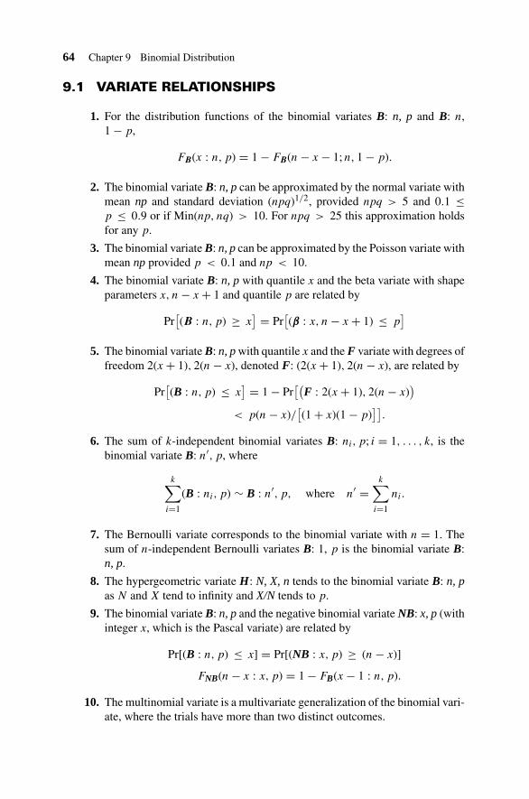
64 Chapter 9 Binomial Distribution
9.1 VARIATE RELATIONSHIPS
1. For the distribution functions of the binomial variates B: n, p and B: n,1 − p,
FB(x : n, p) = 1 − FB(n − x − 1; n, 1 − p).
2. The binomial variate B: n, p can be approximated by the normal variate withmean np and standard deviation (npq)1/2, provided npq > 5 and 0.1 ≤p ≤ 0.9 or if Min(np, nq) > 10. For npq > 25 this approximation holdsfor any p.
3. The binomial variate B: n, p can be approximated by the Poisson variate withmean np provided p < 0.1 and np < 10.
4. The binomial variate B: n, p with quantile x and the beta variate with shapeparameters x, n − x + 1 and quantile p are related by
Pr[(B : n, p) ≥ x
] = Pr[(β : x, n − x + 1) ≤ p
]
5. The binomial variate B: n, p with quantile x and the F variate with degrees offreedom 2(x + 1), 2(n − x), denoted F: (2(x + 1), 2(n − x), are related by
Pr[(B : n, p) ≤ x
] = 1 − Pr[(
F : 2(x + 1), 2(n − x))
< p(n − x)/[(1 + x)(1 − p)
]].
6. The sum of k-independent binomial variates B: ni, p; i = 1, . . . , k, is thebinomial variate B: n′, p, where
k∑i=1
(B : ni, p) ∼ B : n′, p, where n′ =k∑
i=1
ni.
7. The Bernoulli variate corresponds to the binomial variate with n = 1. Thesum of n-independent Bernoulli variates B: 1, p is the binomial variate B:n, p.
8. The hypergeometric variate H: N, X, n tends to the binomial variate B: n, pas N and X tend to infinity and X/N tends to p.
9. The binomial variate B: n, p and the negative binomial variate NB: x, p (withinteger x, which is the Pascal variate) are related by
Pr[(B : n, p) ≤ x] = Pr[(NB : x, p) ≥ (n − x)]
FNB(n − x : x, p) = 1 − FB(x − 1 : n, p).
10. The multinomial variate is a multivariate generalization of the binomial vari-ate, where the trials have more than two distinct outcomes.

9.3 Random Number Generation 65
9.2 PARAMETER ESTIMATION
Parameter Estimator Method/Properties
Bernoulli probability, p x/n Minimum variance unbiased
9.3 RANDOM NUMBER GENERATION
1. Rejection Technique. Select n unit rectangular random numbers. The numberof these that are less than p is a random number of the binomial variate B:n, p.
2. Geometric Distribution Method. If p is small, a faster method may be to addtogether x geometric random numbers until their sum exceeds n − x. Thenumber of such geometric random numbers is a binomial random number.

Chapter 10
Cauchy Distribution
The Cauchy distribution is of mathematical interest due to the absence of definedmoments.
Variate C: a, b.
Range −∞ < x < ∞.
Location parameter a, the median.
Scale parameter b > 0.
Distribution function1
2+ 1
πtan−1
(x − a
b
)
Probability density function
{πb
[1 +
(x − a
b
)2]}−1
Characteristic function exp(iat − |t|b)
Inverse distribution function
(of probability α) a + b[
tan π(α − 1
2
)]Moments Do not exist
Cumulants Do not exist
Mode a
Median a
10.1 NOTE
The Cauchy distribution is unimodal and symmetric, with much heavier tails than thenormal. The probability density function is symmetric about a, with upper and lowerquartiles, a ± b.
The probability density functions of the C: 0, b variate, for selected values of thescale parameter b, are shown in Figure 10.1.
Statistical Distributions, Fourth Edition, by Catherine Forbes, Merran Evans, Nicholas Hastings,and Brian PeacockCopyright © 2011 John Wiley & Sons, Inc.
66

10.2 Variate Relationships 67
Quantile x
0.1
0.2
0.3
0.4
0.5
0.6
−4 −3 −2 −1 43210
b = 2
b = 1
b = 0.5
a = 0
Probabilitydensity
Figure 10.1. Cauchy probability density function C:a,b.
10.2 VARIATE RELATIONSHIPS
The Cauchy variate C: a, b is related to the standard Cauchy variate C: 0, 1 by
C : a, b ∼ a + b(C : 0, 1).
1. The ratio of two independent unit normal variates N1, N2 is the standardCauchy variate C: 0, 1.
(N1/N2) ∼ C : 0, 1.
2. The standard Cauchy variate is a special case of the Student’s t variate withone degree of freedom, t: 1.
3. The sum of n-independent Cauchy variates C : ai, bi with location parametersai, i = 1, . . . , n and scale parameters bi, i = 1, . . . , n is a Cauchy variate C:a, b with parameters the sum of those of the individual variates:
n∑i=1
(C : ai, bi) ∼ C : a, b, where a =n∑
i=1
ai, b =n∑
i=1
bi.
The average of n-independent Cauchy variates C: a, b is the Cauchy C: a, b
variate. Hence the distribution is “stable” and infinitely divisible.
4. The reciprocal of a Cauchy variate C: a, b is a Cauchy variate C : a′, b′, wherea′, b′ are given by
1/(C : a, b) ∼ C : a′, b′, where a′ = a/(a2 + b2), b′ = b/(a2 + b2).

68 Chapter 10 Cauchy Distribution
10.3 RANDOM NUMBER GENERATION
The standard Cauchy variate C: 0, 1 is generated from the unit rectangular variateR by
C : 0, 1 ∼ cot(πR) = tan[π(R − 1
2
)].
10.4 GENERALIZED FORM
Shape parameter m > 0, normalizing constant k.For m = 1, this variate corresponds to the Cauchy variate C: a, b.For a = 0, this variate corresponds to a Student’s t variate with (2m − 1) degrees offreedom, multiplied by b(2m − 1)−1/2.
Probability density function k
[1 +
(x − a
b
)2]−m
, m≥ 1
where k = �(m)/[b�(1/2)�
(m − 1
2
)]Mean a
Median a
Mode a
rth Moment about the mean
⎧⎪⎪⎨⎪⎪⎩
�
(r + 1
2
)�
(m − r + 1
2
)
�(1/r)�(m − 1/r), r even, r < 2m − 1
0, r odd

Chapter 11
Chi-Squared Distribution
Important applications of the chi-squared variate arise from the fact that it is thedistribution of the sum of the squares of a number of normal variates. Where a set ofdata is represented by a theoretical model, the chi-squared distribution can be usedto test the goodness of fit between the observed data points and the values predictedby the model, subject to the differences being normally distributed. A particularlycommon application is the analysis of contingency tables.
Variate χ2 : ν.
Range 0 ≤ x < ∞.
Shape parameter ν, degrees of freedom.
Probability density functionx(ν−2)/2 exp(−x/2)
2ν/2�(ν/2)
where �(ν/2) is the gamma function
with argument ν/2
Moment generating function (1 − 2t)−ν/2, t < 12
Laplace transform of the pdf (1 + 2s)−ν/2, s > − 12
Characteristic function (1 − 2it)−ν/2
Cumulant generating function (−ν/2) log(1 − 2it)
rth Cumulant 2r−1ν(r − 1)!, r ≥ 1
rth Moment about the origin 2rr−1∏i=0
[i + (ν/2)] = 2r�(r + ν/2)
�(ν/2)Mean ν
Variance 2ν
Mode ν − 2, ν ≥ 2
Median ν − 23 (approximately for large ν)
Statistical Distributions, Fourth Edition, by Catherine Forbes, Merran Evans, Nicholas Hastings,and Brian PeacockCopyright © 2011 John Wiley & Sons, Inc.
69
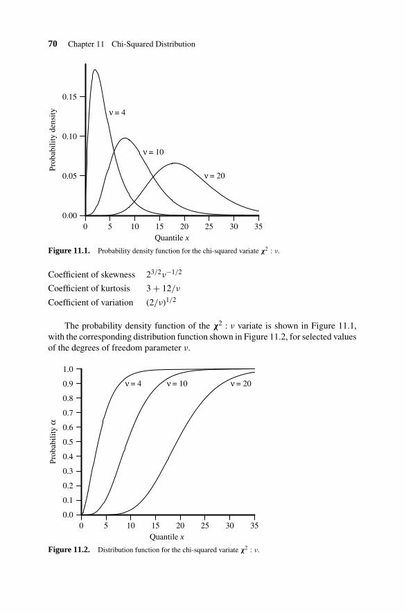
70 Chapter 11 Chi-Squared Distribution
Quantile x
Prob
abili
ty d
ensi
ty
0.00
0.05
0.10
0.15
50 10 15 20 25 30 35
ν = 20
ν = 10
ν = 4
Figure 11.1. Probability density function for the chi-squared variate χ2 : ν.
Coefficient of skewness 23/2ν−1/2
Coefficient of kurtosis 3 + 12/ν
Coefficient of variation (2/ν)1/2
The probability density function of the χ2 : ν variate is shown in Figure 11.1,with the corresponding distribution function shown in Figure 11.2, for selected valuesof the degrees of freedom parameter ν.
Quantile x
Prob
abili
ty α
0.0
0.1
0.2
0.3
0.4
0.5
0.6
0.7
0.8
0.9
1.0
50 10 15 20 25 30 35
ν = 20 ν = 10 ν = 4
Figure 11.2. Distribution function for the chi-squared variate χ2 : ν.

11.1 Variate Relationships 71
11.1 VARIATE RELATIONSHIPS
1. The chi-squared variate with ν degrees of freedom is equal to the gammavariate with scale parameter 2 and shape parameter ν/2, or equivalently istwice the gamma variate with scale parameter 1 and shape parameter ν/2.
χ2 : ν ∼ γ : 2, ν/2
∼ 2(γ : 1, ν/2).
Properties of the gamma variate apply to the chi-squared variate χ2 : ν. Thechi-squared variate χ2: 2 is the exponential variate E: 2.
2. The independent chi-squared variates with ν and ω degrees of freedom,denoted χ2 : ν and χ2 : ω, respectively, are related to the F variate withdegrees of freedom ν, ω, denoted F: ν, ω by
F : ν, ω ∼ (χ2 : ν)/ν
(χ2 : ω)/ω.
3. As ω tends to infinity, ν times the F variate F: ν, ω tends to the chi-squaredvariate χ2 : ν.
χ2 : ν ≈ ν(F : ν, ω) as ω → ∞.
4. The chi-squared variate χ2 : ν is related to the Student’s t variate with ν
degrees of freedom, denoted t: ν, and the independent unit normal variateN: 0, 1 by
t : ν ∼ N : 0, 1
[(χ2 : ν)/ν]1/2 .
5. The chi-squared variate χ2 : ν is related to the Poisson variate with meanx/2, denoted P: x/2, by
Pr[(χ2 : ν) > x] = Pr[(P : x/2) ≤ ((ν/2) − 1)].
Equivalent statements in terms of the distribution function F and inversedistribution function G are
1 − Fχ2 (x : ν) = FP ([(ν/2) − 1] : x/2)
Gχ2 ((1 − α) : ν) = x ⇔ GP (α : x/2) = (ν/2) − 1.
0 ≤ x < ∞; ν/2 a positive integer; 0 < α < 1; α denotes probability.
6. The chi-squared variate χ2 : ν is equal to the sum of the squares of ν-independent unit normal variates, N: 0, 1.
χ2 : ν ∼ν∑
i=1
(N : 0, 1)2i ∼
ν∑i=1
((N : μi, σi) − μi
σi
)2

72 Chapter 11 Chi-Squared Distribution
7. The sum of independent chi-squared variates is also a chi-squared variate:
n∑i=1
(χ2 : νi) ∼ χ2 : ν, where ν =n∑
i=1
νi.
8. The chi-squared variate χ2 : ν for ν large can be approximated by transfor-mations of the normal variate.
χ2 : ν ≈ 12 [(2ν − 1)1/2 + (N : 0, 1)]2
χ2 : ν ≈ ν[1 − 2/(9ν) + [2/(9ν)]1/2(N : 0, 1)]3.
The first approximation of Fisher is less accurate than the second of Wilson–Hilferty.
9. Given n normal variates N: μ, σ, the sum of the squares of their devia-tions from their mean is the variate σ2χ2 : n − 1. Define variates x, s2 asfollows:
x ∼ 1
n
n∑i=1
(N : μ, σ)i, s2 ∼ 1
n
n∑i=1
[(N : μ, σ)i − x
]2.
Then ns2/σ2 ∼ χ2 : n − 1.
10. Consider a set of n1-independent normal variates N: μ1, σ, and a set ofn2-independent normal variates N: μ2, σ (note same σ) and define variatesx1, x2, s
21, s
22 as follows:
x1 ∼ 1
n1
n1∑i=1
(N : μ1, σ)i; s21 ∼ 1
n1
n1∑i=1
[(N : μ1, σ)i − x1
]2
x2 ∼ 1
n2
n2∑j=1
(N : μ2, σ)j; s22 ∼ 1
n2
n2∑j=1
[(N : μ2, σ)j − x2
]2.
Then(n1s
21 + n2s
22
)/σ2 ∼ χ2 : n1 + n2 − 2.
11.2 RANDOM NUMBER GENERATION
For independent N: 0, 1 variates
χ2 : ν ∼ν∑
i=1
(N : 0, 1)2i .
See also the gamma distribution.
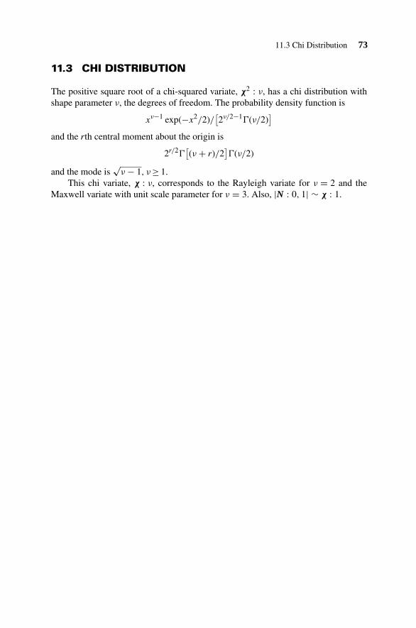
11.3 Chi Distribution 73
11.3 CHI DISTRIBUTION
The positive square root of a chi-squared variate, χ2 : ν, has a chi distribution withshape parameter ν, the degrees of freedom. The probability density function is
xν−1 exp(−x2/2)/[2ν/2−1�(ν/2)
]and the rth central moment about the origin is
2r/2�[(ν + r)/2
]�(ν/2)
and the mode is√
ν − 1, ν ≥ 1.This chi variate, χ : ν, corresponds to the Rayleigh variate for ν = 2 and the
Maxwell variate with unit scale parameter for ν = 3. Also, |N : 0, 1| ∼ χ : 1.
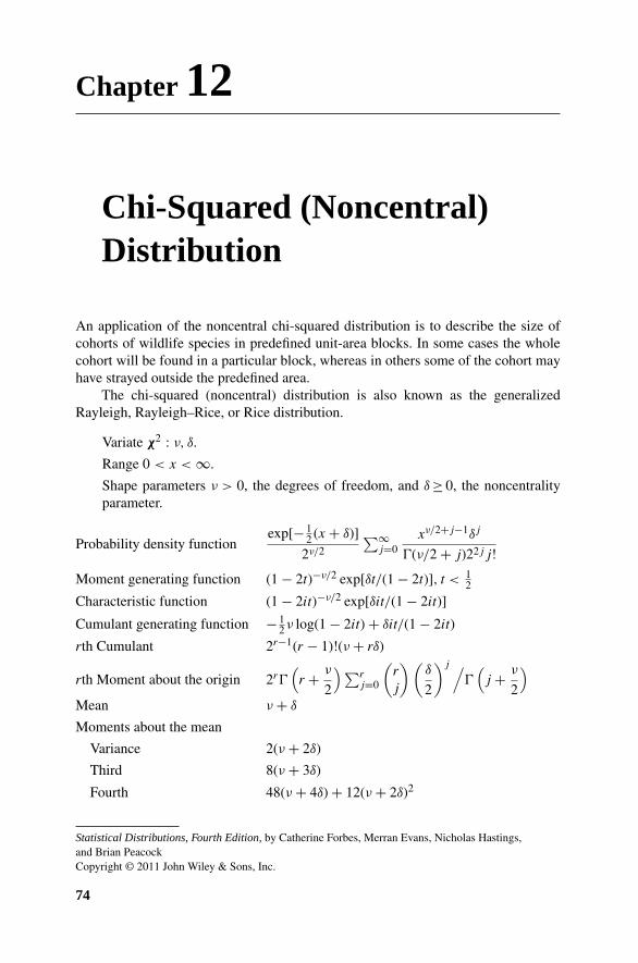
Chapter 12
Chi-Squared (Noncentral)Distribution
An application of the noncentral chi-squared distribution is to describe the size ofcohorts of wildlife species in predefined unit-area blocks. In some cases the wholecohort will be found in a particular block, whereas in others some of the cohort mayhave strayed outside the predefined area.
The chi-squared (noncentral) distribution is also known as the generalizedRayleigh, Rayleigh–Rice, or Rice distribution.
Variate χ2 : ν, δ.
Range 0 < x < ∞.
Shape parameters ν > 0, the degrees of freedom, and δ ≥ 0, the noncentralityparameter.
Probability density functionexp[− 1
2 (x + δ)]
2ν/2
∑∞j=0
xν/2+j−1δj
�(ν/2 + j)22jj!
Moment generating function (1 − 2t)−ν/2 exp[δt/(1 − 2t)], t < 12
Characteristic function (1 − 2it)−ν/2 exp[δit/(1 − 2it)]
Cumulant generating function − 12ν log(1 − 2it) + δit/(1 − 2it)
rth Cumulant 2r−1(r − 1)!(ν + rδ)
rth Moment about the origin 2r�(r + ν
2
) ∑rj=0
(r
j
) (δ
2
)j /�
(j + ν
2
)Mean ν + δ
Moments about the mean
Variance 2(ν + 2δ)
Third 8(ν + 3δ)
Fourth 48(ν + 4δ) + 12(ν + 2δ)2
Statistical Distributions, Fourth Edition, by Catherine Forbes, Merran Evans, Nicholas Hastings,and Brian PeacockCopyright © 2011 John Wiley & Sons, Inc.
74

12.1 Variate Relationships 75
Quantile x
Prob
abili
ty d
ensi
ty
0.00
0.05
0.10
0.15
50 10 15 20 25 30 35
δ = 10
δ = 2
δ = 0.5
ν = 4
Figure 12.1. Probability density function for the (noncentral) chi-squared variate χ2 : ν, δ.
Coefficient of skewness 81/2(ν + 3δ)/(ν + 2δ)3/2
Coefficient of kurtosis 3 + 12(ν + 4δ)/(ν + 2δ)2
Coefficient of variation [2(ν + 2δ)]1/2/(ν + δ)
The probability density function of the χ2 : 4, δ variate is shown in Figure 12.1for selected values of the noncentrality parameter δ.
12.1 VARIATE RELATIONSHIPS
1. Given ν-independent standard normal variates N: 0, 1, then, the noncentralchi-squared variate corresponds to
χ2 : ν, δ∼ν∑
i=1
[(N : 0, 1)i + δi]2∼
ν∑i=1
(N : δi, 1)2,
where δ =ν∑
i=1
δ2i .
2. The sum of n-independent noncentral chi-squared variates χ2 : νi, δi, i =1, . . . , n, is a noncentral chi-squared variate χ2 : ν, δ.
χ2 : ν, δ∼n∑
i=1
(χ2 : νi, δi), where ν =n∑
i=1
νi, δ =n∑
i=1
δi.
3. The noncentral chi-squared variate χ2 : ν, δ with zero noncentrality parameterδ = 0 is the (central) chi-squared variate χ2 : ν.

76 Chapter 12 Chi-Squared (Noncentral) Distribution
4. The standardized noncentral chi-squared variate χ2 : ν, δ tends to the standardnormal variate N: 0, 1, either when ν tends to infinity as δ remains fixed orwhen δ tends to infinity as ν remains fixed.
5. The noncentral chi-squared variate χ2 : ν, δ (for ν even) is related to twoindependent Poisson variates with parameters ν/2 and δ/2, denoted P: ν/2and P: δ/2, respectively, by
Pr[(χ2 : ν, δ) ≤ x] = Pr[[(P : ν/2) − (P : δ/2)] ≥ ν/2].
6. The independent noncentral chi-squared variate χ2 : ν, δ and central chi-squared variate χ2 : ω are related to the noncentral F variate F: ν, ω, δ by
F : ν, ω, δ ∼ (χ2 : ν, δ)/ν
(χ2 : ω)/ω.

Chapter 13
Dirichlet Distribution
The standard or Type I Dirichlet is a multivariate generalization of the beta distribution.
Vector quantile with elements x1, . . . , xk.
Range xi ≥ 0,∑k
i=1 xi ≤ 1.
Parameters ci > 0, i = 1, . . . , k and c0.
Probability density function�
(k∑
i=0
ci
)k∏
i=0
�(ci)
k∏i=1
xci−1i
(1 −
k∑i=1
xi
)c0−1
.
For individual elements (with c = ∑ki=0 ci):
Mean ci/c
Variance ci(c − ci)/[c2(c + 1)]
Covariance −cicj/[c2(c + 1)]
13.1 VARIATE RELATIONSHIPS
1. The elements Xi, i = 1, . . . , k, of the Dirichlet multivariate vector are re-lated to independent standard gamma variates with shape parameters ci, i =0, . . . , k, by
Xi ∼ γ : 1, ci(k∑
j=0(γ : 1, cj)
) , i = 1, . . . , k
Statistical Distributions, Fourth Edition, by Catherine Forbes, Merran Evans, Nicholas Hastings,and Brian PeacockCopyright © 2011 John Wiley & Sons, Inc.
77

78 Chapter 13 Dirichlet Distribution
and independent chi-squared variates with shape parameters 2νi, i =0, . . . , k, by
Xi ∼ χ2 : 2νi
k∑j=0
(χ2 : 2νj)
, i = 1, . . . , k.
2. For k = 1, the Dirichlet univariate is the beta variate β : ν, ω with parametersν = c1 and ω = c0. The Dirichlet variate can be regarded as a multivariategeneralization of the beta variate.
3. The marginal distribution of Xi is the standard beta distribution with param-eters
ν = ci and ω =k∑
j=0
cj − ci.
4. The Dirichlet variate with parameters npi is an approximation to the multi-nominal variate, for npi not too small for every i.
13.2 DIRICHLET MULTINOMIAL DISTRIBUTION
The Dirichlet multinominal distribution is the multivariate generalization of the betabinomial distribution. It is also known as the compound multinomial distribution and,for integer parameters, the multivariate negative hypergeometric distribution.
It arises if the parameters pi, i = 1, . . . , k, of the multinomial distribution followa Dirichlet distribution. It has probability function
n!�
(k∑
j=1cj
)
�
(n +
k∑j=1
cj
) k∏j=1
xj + cj
cj
,
k∑i=1
xi = n, xi ≥ 0.
The mean of the individual elements xi is nci/c, where c = ∑kj=1 cj , and the variances
and covariances correspond to those of a multinomial distribution with pi = ci/c. Themarginal distribution of Xi is a beta binomial.
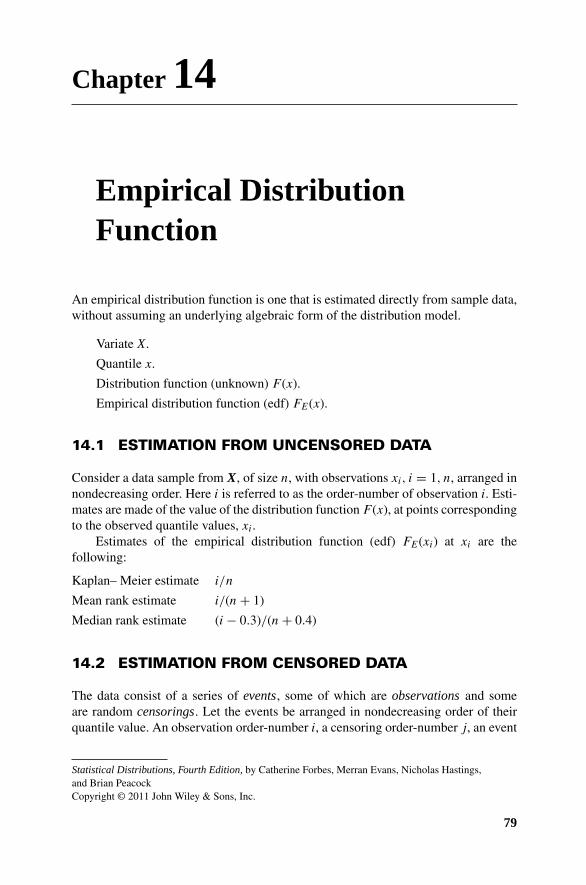
Chapter 14
Empirical DistributionFunction
An empirical distribution function is one that is estimated directly from sample data,without assuming an underlying algebraic form of the distribution model.
Variate X.
Quantile x.
Distribution function (unknown) F (x).
Empirical distribution function (edf) FE(x).
14.1 ESTIMATION FROM UNCENSORED DATA
Consider a data sample from X, of size n, with observations xi, i = 1, n, arranged innondecreasing order. Here i is referred to as the order-number of observation i. Esti-mates are made of the value of the distribution function F (x), at points correspondingto the observed quantile values, xi.
Estimates of the empirical distribution function (edf) FE(xi) at xi are thefollowing:
Kaplan– Meier estimate i/n
Mean rank estimate i/(n + 1)
Median rank estimate (i − 0.3)/(n + 0.4)
14.2 ESTIMATION FROM CENSORED DATA
The data consist of a series of events, some of which are observations and someare random censorings. Let the events be arranged in nondecreasing order of theirquantile value. An observation order-number i, a censoring order-number j, an event
Statistical Distributions, Fourth Edition, by Catherine Forbes, Merran Evans, Nicholas Hastings,and Brian PeacockCopyright © 2011 John Wiley & Sons, Inc.
79

80 Chapter 14 Empirical Distribution Function
order-number e, and a modified (observation) order-number mi are used. A modifiedorder-number is an adjusted observation order-number that allows for the censoreditems. The modified order-numbers and then the distribution function value at quantilexi are calculated with the modified order-number mi replacing the observation order-number i in the median rank equation above.
i = observation order-number (excludes censorings)
I = total number of observations (excludes censorings)
e = event order-number (observations and censorings)
n = total number of events (observations and censorings)
j = censoring order-number
ei = event-number of observation i
ej = event-number of censoring j
mi = modified order-number of observation i
C(i) = set of censoring occurring at or after observation i − 1
and before observation i (this set may be empty)
xi = the quantile value (e.g., age at failure) for observation i
xe = the quantile value for event e, which may be an observation
or a censoring
xj = the quantile value for censoring j
m∗i = n + 1 − mi
e∗i = n + 1 − ei
αj = the proportion of the current interobservation interval
that has elapsed when censoring j occurs
x0 = m0 = e0 = 0
For censoring j in the set C(i), αj is defined by
αj = (xj − xi−1)/(xi − xi−1).
αj is the proportion of the interval between observation i − 1 and observation i,which elapses before censoring j occurs. The method used is described in Bartlett andHastings (1998). The Herd-Johnson method described by d’Agostino and Stephens(1986) is equivalent to assuming that all values of αj are zero.
The formula for the modified order-number is
mi − mi−1 = m∗i−1
⎛⎝1 − e∗
i
e∗i−1
∏C(i)
e∗j + 1 − αj
e∗j − αj
⎞⎠ .
Here, the product is taken over suspensions in the set C(i). If this set is empty theproduct term has value 1, and
mi − mi−1 = m∗i−1/e
∗i−1
FE(xi) = (mi − 0.3)/(n + 0.4).
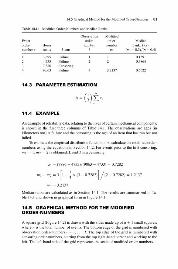
14.5 Graphical Method for the Modified Order-Numbers 81
Table 14.1: Modified Order-Numbers and Median Ranks
Observation ModifiedEvent order- order- Medianorder- Hours number number rank, F (x)number e run, x Status i mi (mi − 0.3)/(n + 0.4)
1 3,895 Failure 1 1 0.15912 4,733 Failure 2 2 0.38643 7,886 Censoring4 9,063 Failure 3 3.2137 0.6622
14.3 PARAMETER ESTIMATION
μ =(
1
I
) N∑e=1
xe
14.4 EXAMPLE
An example of reliability data, relating to the lives of certain mechanical components,is shown in the first three columns of Table 14.1. The observations are ages (inkilometers run) at failure and the censoring is the age of an item that has run but notfailed.
To estimate the empirical distribution function, first calculate the modified order-numbers using the equations in Section 14.2. For events prior to the first censoring,m1 = 1, m2 = 2 is obtained. Event 3 is a censoring.
α3 = (7886 − 4733)/(9063 − 4733) = 0.7282
m3 − m2 = 3
[1 − 1
3× (3 − 0.7282)
] /(2 − 0.7282) = 1.2137
m3 = 3.2137
Median ranks are calculated as in Section 14.1. The results are summarized in Ta-ble 14.1 and shown in graphical form in Figure 14.1.
14.5 GRAPHICAL METHOD FOR THE MODIFIEDORDER-NUMBERS
A square grid (Figure 14.2) is drawn with the sides made up of n + 1 small squares,where n is the total number of events. The bottom edge of the grid is numbered withobservation order-numbers i = 1, . . . , I. The top edge of the grid is numbered withcensoring order-numbers, starting from the top right-hand corner and working to theleft. The left-hand side of the grid represents the scale of modified order-numbers.
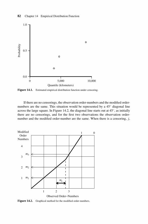
82 Chapter 14 Empirical Distribution Function
Quantile (kilometers)
Prob
abili
ty
0.0
0.5
1.0
0 5,000 10,000
Figure 14.1. Estimated empirical distribution function under censoring.
If there are no censorings, the observation order-numbers and the modified order-numbers are the same. This situation would be represented by a 45◦ diagonal lineacross the large square. In Figure 14.2, the diagonal line starts out at 45◦, as initiallythere are no censorings, and for the first two observations the observation order-number and the modified order-number are the same. When there is a censoring, j,
Observed Order−Numbers
αj
321
1
2
3
4
01
m1
m2
m3
ModifiedOrder
Numbers
Figure 14.2. Graphical method for the modified order-numbers.

14.6 Model Accuracy 83
between observation i − 1 and observation i, the censoring is indicated by a dottedvertical line placed a proportion αj between observations. The vertical dotted line i
between observation 2 and observation 3 illustrates this. The gradient of the diag-onal line increases at each censoring, becoming directed toward the correspondingcensoring order-number on the top scale of the square. In the example, there is onlyone censoring, so the gradient of the diagonal line increases only once. The modifiedorder-numbers are read off from the left-hand vertical scale, by drawing horizontallines across from the points where the vertical lines through the observation numbersintersect the diagonal line.
14.6 MODEL ACCURACY
For any given distribution model, let FM(xi) be the distribution function value atquantile xi, where the edf value is FE(xi). Let q2
i be the square of the differencebetween the model value FM(xi) and the edf value FE(xi).
q2i = [FM(xi) − FE(xi)]
2.
The mean square error between the edf points and the model distribution function isgiven by the Cramer–von Mises statistic:
Q2 =(
1
I
) I∑i=1
q2i .
A, the model accuracy, is defined (in percentage terms) by
A = 100(1 − Q).
If the edf points all lie exactly on the model distribution function curve, the modelaccuracy is 100%.
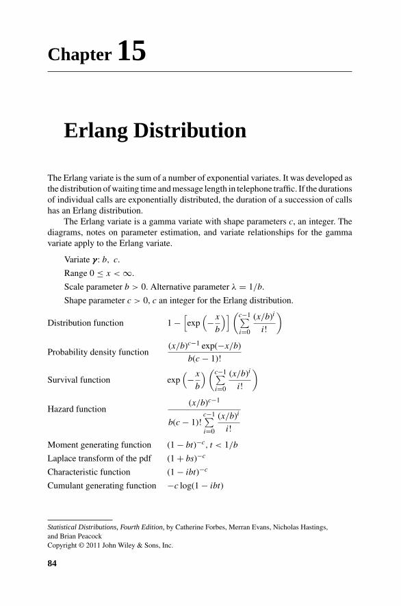
Chapter 15
Erlang Distribution
The Erlang variate is the sum of a number of exponential variates. It was developed asthe distribution of waiting time and message length in telephone traffic. If the durationsof individual calls are exponentially distributed, the duration of a succession of callshas an Erlang distribution.
The Erlang variate is a gamma variate with shape parameters c, an integer. Thediagrams, notes on parameter estimation, and variate relationships for the gammavariate apply to the Erlang variate.
Variate γ: b, c.
Range 0 ≤ x < ∞.
Scale parameter b > 0. Alternative parameter λ = 1/b.
Shape parameter c > 0, c an integer for the Erlang distribution.
Distribution function 1 −[exp
(−x
b
)] (c−1∑i=0
(x/b)i
i!
)
Probability density function(x/b)c−1 exp(−x/b)
b(c − 1)!
Survival function exp(−x
b
) (c−1∑i=0
(x/b)i
i!
)
Hazard function(x/b)c−1
b(c − 1)!c−1∑i=0
(x/b)i
i!
Moment generating function (1 − bt)−c, t < 1/b
Laplace transform of the pdf (1 + bs)−c
Characteristic function (1 − ibt)−c
Cumulant generating function −c log(1 − ibt)
Statistical Distributions, Fourth Edition, by Catherine Forbes, Merran Evans, Nicholas Hastings,and Brian PeacockCopyright © 2011 John Wiley & Sons, Inc.
84
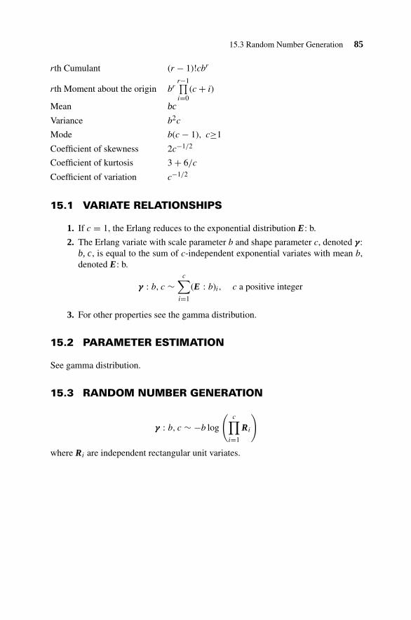
15.3 Random Number Generation 85
rth Cumulant (r − 1)!cbr
rth Moment about the origin brr−1∏i=0
(c + i)
Mean bc
Variance b2c
Mode b(c − 1), c≥1
Coefficient of skewness 2c−1/2
Coefficient of kurtosis 3 + 6/c
Coefficient of variation c−1/2
15.1 VARIATE RELATIONSHIPS
1. If c = 1, the Erlang reduces to the exponential distribution E: b.
2. The Erlang variate with scale parameter b and shape parameter c, denoted γ:b, c, is equal to the sum of c-independent exponential variates with mean b,denoted E: b.
γ : b, c ∼c∑
i=1
(E : b)i, c a positive integer
3. For other properties see the gamma distribution.
15.2 PARAMETER ESTIMATION
See gamma distribution.
15.3 RANDOM NUMBER GENERATION
γ : b, c ∼ −b log
(c∏
i=1
Ri
)
where Ri are independent rectangular unit variates.
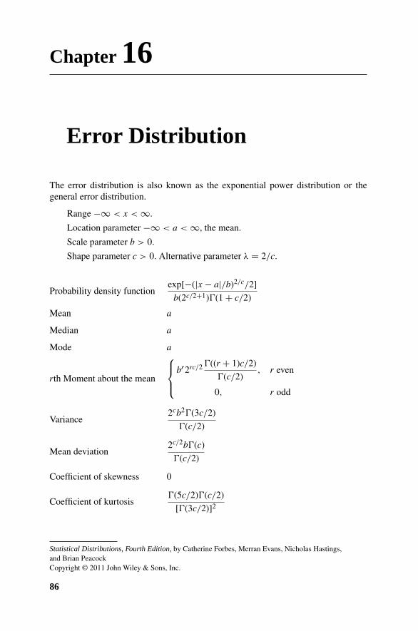
Chapter 16
Error Distribution
The error distribution is also known as the exponential power distribution or thegeneral error distribution.
Range −∞ < x < ∞.
Location parameter −∞ < a < ∞, the mean.
Scale parameter b > 0.
Shape parameter c > 0. Alternative parameter λ = 2/c.
Probability density functionexp[−(|x − a|/b)2/c/2]
b(2c/2+1)�(1 + c/2)
Mean a
Median a
Mode a
rth Moment about the mean
⎧⎪⎨⎪⎩
br2rc/2 �((r + 1)c/2)
�(c/2), r even
0, r odd
Variance2cb2�(3c/2)
�(c/2)
Mean deviation2c/2b�(c)
�(c/2)
Coefficient of skewness 0
Coefficient of kurtosis�(5c/2)�(c/2)
[�(3c/2)]2
Statistical Distributions, Fourth Edition, by Catherine Forbes, Merran Evans, Nicholas Hastings,and Brian PeacockCopyright © 2011 John Wiley & Sons, Inc.
86
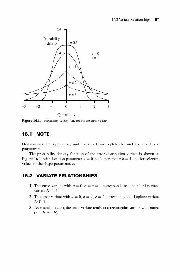
16.2 Variate Relationships 87
Quantile x
0.2
0.4
0.6
−3 −2 −1 3210
c = 3
c = 2
c = 1
c = 0.5Probability
density
a = 0b = 1
Figure 16.1. Probability density function for the error variate.
16.1 NOTE
Distributions are symmetric, and for c > 1 are leptokurtic and for c < 1 areplatykurtic.
The probability density function of the error distribution variate is shown inFigure 16.1, with location parameter a = 0, scale parameter b = 1 and for selectedvalues of the shape parameter, c.
16.2 VARIATE RELATIONSHIPS
1. The error variate with a = 0, b = c = 1 corresponds to a standard normalvariate N: 0, 1.
2. The error variate with a = 0, b = 12 , c = 2 corresponds to a Laplace variate
L: 0, 1.
3. As c tends to zero, the error variate tends to a rectangular variate with range(a − b, a + b).

Chapter 17
Exponential Distribution
This is a distribution of the time to an event when the probability of the event occurringin the next small time interval does not vary through time. It is also the distribution ofthe time between events when the number of events in any time interval has a Poissondistribution.
The exponential distribution has many applications. Examples include the timeto decay of a radioactive atom and the time to failure of components with constantfailure rates. It is used in the theory of waiting lines or queues, which are found inmany situations: from the gates at the entrance to toll roads through the time takenfor an answer to a telephone enquiry, to the time taken for an ambulance to arrive atthe scene of an accident. For exponentially distributed times, there will be many shorttimes, fewer longer times, and occasional very long times. See Chapter 38.
The exponential distribution is also known as the negative exponential distribu-tion.
Variate E: b.
Range 0 ≤ x < +∞.
Scale parameter b > 0, the mean.
Alternative parameter λ, the hazard function (hazard rate), λ = 1/b.
Distribution function 1 − exp(−x/b)
Probability density function (1/b) exp(−x/b) = λ exp(−λx)
Inverse distribution function b log[1/(1 − α)] = −b log(1 − α)
(of probability α)
Survival function exp(−x/b)
Inverse survival function b log(1/α) = −b log(α)
(of probability α)
Hazard function 1/b = λ
Statistical Distributions, Fourth Edition, by Catherine Forbes, Merran Evans, Nicholas Hastings,and Brian PeacockCopyright © 2011 John Wiley & Sons, Inc.
88
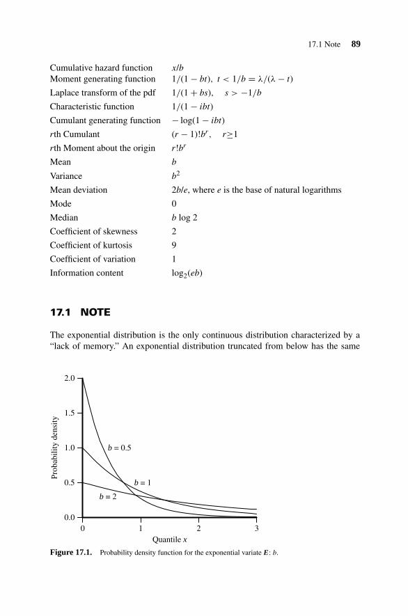
17.1 Note 89
Cumulative hazard function x/bMoment generating function 1/(1 − bt), t < 1/b = λ/(λ − t)
Laplace transform of the pdf 1/(1 + bs), s > −1/b
Characteristic function 1/(1 − ibt)
Cumulant generating function − log(1 − ibt)
rth Cumulant (r − 1)!br, r≥1
rth Moment about the origin r!br
Mean b
Variance b2
Mean deviation 2b/e, where e is the base of natural logarithms
Mode 0
Median b log 2
Coefficient of skewness 2
Coefficient of kurtosis 9
Coefficient of variation 1
Information content log2(eb)
17.1 NOTE
The exponential distribution is the only continuous distribution characterized by a“lack of memory.” An exponential distribution truncated from below has the same
Quantile x
Prob
abili
ty d
ensi
ty
0.0
0.5
1.0
1.5
2.0
210 3
b = 2
b = 1
b = 0.5
Figure 17.1. Probability density function for the exponential variate E: b.

90 Chapter 17 Exponential Distribution
Quantile x
Prob
abili
ty α
0.0
0.5
1.0
210 3
b = 2
b = 1
b = 0.5
Figure 17.2. Distribution function for the exponential variate E:b.
distribution with the same parameter b. The geometric distribution is its discreteanalogue. The hazard rate is constant.
The probability density function of the E : b variate is shown in Figure 17.1 forselected values of the scale parameter, b. The corresponding distribution function andcumulative hazard function are shown in Figures 17.2 and 17.3, respectively.
Mean
Cum
ulat
ive
haza
rd
0
1
0 bx
Figure 17.3. Cumulative hazard function for the exponential variate E: b.

17.2 Variate Relationships 91
17.2 VARIATE RELATIONSHIPS
(E : b)/b ∼ E : 1, the unit exponential variate.
1. The exponential variate E: b is a special case of the gamma variate γ: b, c
corresponding to shape parameter c = 1.
E : b ∼ γ : b, 12. The exponential variate E: b is a special case of the Weibull variate W: b, c
corresponding to shape parameter c = 1.
E : b ∼ W : b, 1
E: 1 is related to Weibull variate W: b, c
b(E : 1)1/c ∼ W : b, c.
3. The exponential variate E: b is related to the unit rectangular variate R by
E : b ∼ −b log R.
4. The sum of c-independent exponential variates, E: b, is the Erlang (gamma)variate γ: b, c, with integer parameter c.
c∑i=1
(E : b)i ∼ γ : b, c
5. The difference of the two independent exponential variates, (E : b)1 and(E : b)2, is the Laplace variate with parameters 0, b, denoted L: 0, b.
L : 0, b ∼ (E : b)1 − (E : b)2
If L: a, b is the Laplace variate, E : b ∼ |(L : a, b) − a|.6. The exponential variate E: b is related to the standard power function variate
with shape parameter c, here denoted X: c, for c = 1/b
X : c ∼ exp(−E : b) for c = 1/b
and the Pareto variate with shape parameter c, here denoted X: a, c for c = 1/b, by
X : a, c ∼ a exp(E : b) for c = 1/b.
7. The exponential variate E: b is related to the Gumbel extreme value variateV: a,b by
V : a, b ∼ a − log(E : b).
8. Let Y be a random variate with a continuous distribution function Fγ . Thenthe standard exponential variate E: 1 corresponds to E : 1 ∼ − log(1 − FY ).

92 Chapter 17 Exponential Distribution
17.3 PARAMETER ESTIMATION
Parameter Estimator Method/Properties
b x Unbiased, maximum likelihood
17.4 RANDOM NUMBER GENERATION
Random numbers of the exponential variate E: b can be generated from randomnumbers of the unit rectangular variate R using the relationship
E : b ∼ −b log R.

Chapter 18
Exponential Family
Variate can be discrete or continuous and uni- or multidimensional.Parameter θ can be uni- or multidimensional.The exponential family is characterized by having a pdf or pf of the form
exp[A(θ) · B(x) + C(x) + D(θ)
].
18.1 MEMBERS OF THE EXPONENTIAL FAMILY
These include the univariate Bernoulli, binomial, Poisson, geometric, gamma,normal, inverse Gaussian, logarithmic, Rayleigh, and von Mises distributions. Mul-tivariate distributions include the multinomial, multivariate normal, Dirichlet, andWishart.
18.2 UNIVARIATE ONE-PARAMETER EXPONENTIALFAMILY
The natural exponential family has B(x) = x, with A(θ) the natural or canonicalparameter.
For A(θ) = θ:
Probability (density) function exp[θx + C(x) + D(θ)
]Characteristic function exp
[D(θ) − D(θ + it)
]Cumulant generating function D(θ) − D(θ + it)
rth Cumulant − dr
dθrD(θ)
Statistical Distributions, Fourth Edition, by Catherine Forbes, Merran Evans, Nicholas Hastings,and Brian PeacockCopyright © 2011 John Wiley & Sons, Inc.
93

94 Chapter 18 Exponential Family
Particular cases are:
Binomial B: n, p for θ = p
A(θ) = log[θ/(1 − θ)] = log(p/q), B(x) = x
C(x) = log
(n
x
)
D(θ) = n log(1 − θ) = n log q
Gamma γ: b, c, for θ = 1/b scale parameter
A(θ) = −θ = −1/b, B(x) = x
C(x) = (c − 1) log x
D(θ) = c log θ − log �(c) = −c log b − log �(c)
Inverse Gaussian I: μ, λ, for θ = μ,
A(θ) = − λ
2θ2 = − λ
2μ2 , B(x) = x
C(x) = − 12
[log
(2π x3
λ
)+ λ
x
]
D(θ) = λ
θ= λ
μ
Negative binomial NB: x, p, for θ = p
A(θ) = log(1 − θ) = log(q), B(y) = y
C(y) = log
(x + y − 1
x − 1
)
D(θ) = x log(θ) = x log(p)
Normal N: μ, 1, for θ = μ,
A(θ) = θ
σ2 , B(x) = x
C(x) = −1
2
[log 2(πσ2) + x2
σ2
]
D(θ) = − μ2
2σ2
18.4 Generalized Exponential Distributions 95
Poisson P: λ, for θ = λ,
A(θ) = log θ = log λ, B(x) = x
C(x) = − log(x!)
D(θ) = −θ = −λ
Families of distributions obtained by sampling from one-parameter exponential fam-ilies are themselves one-parameter exponential families.
18.3 PARAMETER ESTIMATION
The shared important properties of exponential families enable estimation by like-lihood methods, using computer programs such as GenStat (www.vsni.co.uk),R (www.r-project.org), or Stata (www.stata.com).
18.4 GENERALIZED EXPONENTIAL DISTRIBUTIONS
All of the pdfs (or pfs) for the exponential family of distributions satisfy the property
∂f
∂x= −g(x)f (x)
h(x), (18.1)
where g(x) is a polynomial of degree at most one, and h(x) is a polynomial of degreeat most two.
Lye and Martin (1993) propose the univariate generalized exponential family ofdistributions having densities satisfying Equation (18.1) but where the functions g(x)and h(x) are not constrained to low order polynomial functions.
Generalized Student’s t Distribution
In particular, Lye and Martin propose the generalized Student’s t distribution, where
g(x) =M−1∑i=0
αixi
and
h(x) = γ2x2.
γ2 is the “degrees of freedom” parameter. When M = 6, the pdf has the form
f (x) = exp
[θ1 tan−1(x/γ) + θ2 log(γ2 + x2) +
6∑i=3
θixi−2 − η
],
96 Chapter 18 Exponential Family
for −∞ < x < ∞, where
η =∫ ∞
−∞exp
[θ1 tan−1(u/γ) + θ2 log(γ2 + u2) +
6∑i=3
θiui−2
]du
is the normalizing constant.
Variate Relationships
The generalized Student’s t variate is denoted by GET : γ, α0, α1, α2, α3, α4, α5 andsatisfies
θ1 = −α0
γ+ γα2 − γ3α4
θ2 = −α1
2+ γ2α3
2− γ4α5
2
θ3 = −α2 + γ2α4
θ4 = −α3
2+ γ2α5
2
θ5 = −α4
3
θ6 = −α5
4.
1. The standard Student’s t variate t: is a special case of the generalized Student’st variate GET with ν = γ2 degrees of freedom where θ2 = −(1 + γ2) and θ1 = θ3 =θ4 = θ5 = θ6 = 0.
2. The Cauchy variate C: is a special case of the generalized Student’s t variateGET with θ2 = −2 and θ1 = θ3 = θ4 = θ5 = θ6 = 0.
3. The standard Normal variate N : μ, σ2 is a special case of the generalized Stu-dent’s t variate GET with θ1 = θ2 = θ5 = θ6 = 0 and θ3 = μ/σ2 and θ4 = −1/(1σ2).
Generalized Exponential Normal Distribution
The generalized exponential normal variate GEN is defined as a special case of thegeneralized exponential variate with θ1 = θ2 = 0.
Generalized Lognormal Distribution
In particular, Lye and Martin propose the generalized lognormal distribution, where
g(x) = α0 log(x) +M−1∑i=1
αiui−1,

18.4 Generalized Exponential Distributions 97
and
h(x) = x.
When M = 6, the pdf has the form
f (x) = exp
[θ1(log(x))2 + θ2 log(x) +
6∑i=1
θixi−2
],
for x > 0, where
η =∫ ∞
0exp
[θ1(log(u))2 + θ2 log(x) +
6∑i=1
θiui−2
]du
is the normalizing constant.
Variate Relationships
GEL : θ1 = −α0/2, θ2 = −α1
θj+1 = −αj/(j − 1), for j = 2, 3, 4, 5.
1. The standard lognormal variate L : m, σ is a special case of the generalizedexponential lognormal variate GEL with parameters θ1 = 1/(2σ2), θ2 = − log m/σ2,and all thetaj = 0, for j = 3, 4, 5, and 6.
2. The gamma distribution variate γ : b, c is a special case of the generalizedexponential lognormal variate GEL with parameters θ2 = (c − 1), θ3 = −1/b, andall θj = 0, for j = 1, 4, 5, and 6.
3. The Rayleigh distribution variate X : b is a special case of the generalizedexponential lognormal variate GEL with parameters θ2 = 1, θ4 = −1/(2b2), and allθj = 0, for j = 1, 3, 5, and 6.

Chapter 19
Extreme Value (Gumbel)Distribution
The extreme value distribution was developed as the distribution of the largest of anumber of values and was originally applied to the estimation of flood levels. It hassince been applied to the estimation of the magnitude of earthquakes. The distributionmay also be applied to the study of athletic and other records.
We consider the distribution of the largest extreme. Reversal of the sign of x givesthe distribution of the smallest extreme. This is the Type I, the most common of threeextreme value distributions, known as the Gumbel distribution.
Variate V : a, b.
Range −∞ < x < +∞.
Location parameter a, the mode.
Scale parameter b > 0.
Distribution function exp{ − exp
[ − (x − a)/b]}
Probability density function (1/b) exp[−(x−a)/b
]× exp{ − exp
[ − (x−a)/b]}
Inverse distribution function a − b log[
log(1/α)]
(of probability α)
Inverse survival function a − b log{
log[1/(1 − α)
]}(of probability α)
Hazard functionexp
[ − (x − a)/b]
b(
exp{
exp[ − (x − a)/b
]} − 1)
Moment generating function exp(at)�(1 − bt), t < 1/b
Characteristic function exp(iat)�(1 − ibt)
Statistical Distributions, Fourth Edition, by Catherine Forbes, Merran Evans, Nicholas Hastings,and Brian PeacockCopyright © 2011 John Wiley & Sons, Inc.
98

19.1 Note 99
Mean a − b�′(1)
�′(1) = −0.57722 is the first derivativeof the gamma function �(n)with respect to n at n = 1.
Variance b2π2/6
Coefficient of skewness 1.139547
Coefficient of kurtosis 5.4
Mode a
Median a − b log(log 2)
19.1 NOTE
Extreme value variates correspond to the limit, as n tends to infinity, of the maximumvalue of n-independent random variates with the same continuous distribution. Log-arithmic transformations of extreme value variates of Type II (Frechet) and Type III(Weibull) correspond to Type I Gumbel variates.
Figure 19.1 shows the probability density function for the V : a, b variate, whileFigures 19.2 and 19.3 display the corresponding distribution and hazard function,respectively.
Quantile x
a−3b a−b a a+b a+3b a+5b
0.1
0.2
0.3
0.4
0.5
Probabilitydensity
Figure 19.1. Probability density function for the extreme value variate V: a, b (largest extreme).

100 Chapter 19 Extreme Value (Gumbel) Distribution
Quantile x
0.5
1.0
a−3b a−b a a+b a+3b
0.368
Probability
α
Figure 19.2. Distribution function for the extreme value variate V: a, b (largest extreme).
19.2 VARIATE RELATIONSHIPS
((V : a, b) − a)/b ∼ V : 0, 1 is the standard Gumbel extreme value variate.
1. The Gumbel extreme value variate V: a, b is related to the exponential variateE: b by
Quantile x
a−3b a−b a a+b a+3b
Hazard
1
Figure 19.3. Hazard function for the extreme value variate V: a, b (largest extreme).

19.4 Random Number Generation 101
V : a, b = a − log(E : b).
2. Let (E : b)i, i = 1, . . . , n, be independent exponential variates with scale pa-rameter b. For large n,
(E : b)n+a−b log(m) ≈ V : a, b for m = 1, 2, . . .
3. The standard extreme value variate V: 0, 1 is related to the Weibull variate W:b, c by
−c log[(W : b, c)/b] ∼ V : 0, 1.
The extreme value distribution is also known as the “log-Weibull” distribution and isan approximation to the Weibull distribution for large c.
4. The difference of the two independent extreme value variates (V : a, b)1 and(V : a, b)2 is the logistic variate with parameters 0 and b, here denoted X: 0, b,
X : 0, b ∼ (V : a, b)1 − (V : a, b)2.
5. The standard extreme value variate, V: 0, 1 is related to the Pareto variate,here denoted X: a, c by
X : a, c ∼ a{1 − exp[− exp(−V : 0, 1)]}1/c
and the standard power function variate, here denoted X: 0, c by
X : 0, c ∼ exp{− exp[−(V : 0, 1)/c]}.
19.3 PARAMETER ESTIMATION
By the method of maximum likelihood, the estimators a, b are the solutions of thesimultaneous equations
b = x −
n∑i=1
xi exp(
−xi
b
)∑n
i=1 exp(− xi
b
)
a = −b log
[1
n
n∑i=1
exp
(−xi
b
)].
19.4 RANDOM NUMBER GENERATION
Let R denote a unit rectangular variate. Random numbers of the extreme value variateV: a, b can be generated using the relationship
V : a, b ∼ a − b log(− log R).
Chapter 20
F (Variance Ratio) orFisher–Snedecor Distribution
The F variate is the ratio of two chi-squared variates. Chi-squared is the distributionof the variance between data and a theoretical model. The F distribution provides abasis for comparing the ratios of subsets of these variances associated with differentfactors.
Many experimental scientists make use of the technique called analysis of vari-ance. This method identifies the relative effects of the “main” variables and interac-tions between these variables. The F distribution represents the ratios of the variancesdue to these various sources. For example, a biologist may wish to ascertain the rela-tive effects of soil type and water on the yield of a certain crop. The F ratio would beused to compare the variance due to soil type and that due to amount of watering withthe residual effects due to other possible causes of variation in yield. The interactionbetween watering and soil type can also be assessed. The result will indicate whichfactors, if any, are a significant cause of variation.
Variate F : ν, ω.
Range 0 ≤ x < ∞.
Shape parameters ν, ω, positive integers, referred to as “numerator” and “denom-inator” degrees of freedom, respectively.
Probability density function�[(ν + ω)/2](ν/ω)ν/2x(ν−2)/2
�(ν/2)�(ω/2)[1 + (ν/ω)x
](ν+ω)/2
rth Moment about the origin(ω/ν)r�(ν/2 + r)�(ω/2 − r)
�(ν/2)�(ω/2), ω > 2r
Meanω
ω − 2, ω > 2
Statistical Distributions, Fourth Edition, by Catherine Forbes, Merran Evans, Nicholas Hastings,and Brian PeacockCopyright © 2011 John Wiley & Sons, Inc.
102

20.1 Variate Relationships 103
Quantile x
Prob
abili
ty d
ensi
ty
432100.0
0.2
0.4
0.6
0.8
1.0
1.2
ν = 4
ν = 10
ν = 40 ω = 40
Figure 20.1. Probability density function for the F variate F : ν, ω.
Variance2ω2(ν + ω − 2)
ν(ω − 2)2(ω − 4), ω > 4
Modeω(ν − 2)
ν(ω + 2), ν > 2
Coefficient of skewness(2ν + ω − 2)[8(ω − 4)]1/2
ν1/2(ω − 6)(ν + ω − 2)1/2 , ω > 6
Coefficient of kurtosis 3 + 12[(ω − 2)2(ω − 4)+ν(ν + ω − 2)(5ω − 22)]
ν(ω − 6)(ω − 8)(ν + ω − 2), ω>8
Coefficient of variation
[2(ν + ω − 2)
ν(ω − 4)
]1/2
, ω > 4
The probability density function of the F : ν, 40 variate is shown in Figure 20.1,for selected values of the numerator degrees of freedom parameter, ν. The correspond-ing distribution functions are shown in Figure 20.2.
20.1 VARIATE RELATIONSHIPS
1. The quantile of the variate F : ν, ω at probability level 1 − α is the reciprocalof the quantile of the variate F : ω, ν at probability level α. That is,
GF (1 − α : ν, ω) = 1/GF (α : ω, ν)

104 Chapter 20 F (Variance Ratio) or Fisher–Snedecor Distribution
Quantile x
Prob
abili
ty α
432100.0
0.2
0.4
0.6
0.8
1.0
ν =
4 ν
= 1
0ν
= 4
0
ω = 40
Figure 20.2. Distribution function for the F variate F : ν, ω.
where GF (α : ν, ω) is the inverse distribution function of F : ν, ω at probabilitylevel α.
2. The variate F : ν, ω is related to the independent chi-squared variates χ2 : ν
and χ2 : ω by
F : ν, ω ∼ (χ2 : ν)/ν
(χ2 : ω)/ω.
3. As the degrees of freedom ν and ω increase, the F : ν, ω variate tends tonormality.
4. The variate F : ν, ω tends to the chi-squared variate χ2 : ν as ω tends toinfinity:
F : ν, ω ≈ (1/ν)(χ2 : ν) as ω → ∞.
5. The quantile of the variate F: 1, ω at probability level α is equal to the squareof the quantile of the Student’s t variate t : ω at probability level 1
2 (1 + α). That is,
GF (α : 1, ω) =[Gt
(1
2(1 + α) : ω
)]2
.
where G is the inverse distribution function. In terms of the inverse survival functionthe relationship is
ZF (α : 1, ω) =[Zt
(1
2α : ω
)]2
.
20.1 Variate Relationships 105
6. The variate F : ν, ω and the beta variate β : w/2, ν/2 are related by
Pr[(F : ν, ω) > x] = Pr[(β : ω/2, ν/2) ≤ ω/(ω + νx)]
= SF (x : ν, ω)
= Fβ([ω/(ω + νx)] : ω/2, ν/2)
where S is the survival function and F is the distribution function. Hence the inversesurvival function ZF (α : ν, ω) of the variate F : ν, ω and the inverse distributionfunction Gβ(α : ω/2, ν/2) of the beta variate β : ω/2, ν/2 are related by
ZF (α : ν, ω) = GF ((1 − α) : ν, ω)
= (ω/ν){[1/Gβ(α : ω/2, ν/2)] − 1}
where α denotes probability.
7. The variate F : ν, ω and the inverted beta variate Iβ : ν/2, ω/2 are relatedby
F : ν, ω ∼ (ω/v)(Iβ : ν/2, ω/2).
8. Consider two sets of independent normal variates (N : μ1, σ1)i; i =1, . . . , n1 and (N : μ2, σ2)j; j = 1, . . . , n2. Define variates x1, x2, s2
1, s22 as follows:
x1 =n1∑i=1
(N : μ1, σ1)i/n1, x2 =n2∑
j=1
(N : μ2, σ2)j/n2
s21 =
n1∑i=m
[(N : μ1, σ1)i − x1]2/n1
s22 =
n2∑j=1
[(N : μ2, σ2)j − x2]2/n2.
Then
F : n1, n2 ∼ n1s21/(n1 − 1)σ2
1
n2s22/(n2 − 1)σ2
2
.
9. The variate F : ν, ω is related to the binomial variate with Bernoulli trialparameter 1
2 (ω + ν − 2) and Bernoulli probability parameter p by
Pr
[(F : ν, ω) <
ωp
ν(1 − p)
]= 1 − Pr
[(B :
1
2(ω + ν − 2), p
)≤ 1
2(ν − 2)
]
where ω + ν is an even integer.

106 Chapter 20 F (Variance Ratio) or Fisher–Snedecor Distribution
10. The ratio of two independent Laplace variates, with parameters 0 and b,denoted (L : 0, b)i, i = 1, 2 is related to the F: 2, 2 variate by
F : 2, 2 ∼ |(L : 0, b)1||(L : 0, b)2| .

Chapter 21
F (Noncentral) Distribution
Variate F: ν, ω, δ.
Range 0 < x < ∞.
Shape parameters ν, ω, positive integers are the degrees of freedom, and δ > 0the noncentrality parameter.
Probability density function kexp(−δ/2)νν/2ωω/2x(ν−2)/2
B(ν/2, ω/2)(ω + νx)(ν+ω)/2 ,
where k = 1 +∞∑
j=1
((νδx)/2
ω + νx
)j
× (ν + ω)(ν + ω + 2)(ν + ω + 2j − 2)
j!ν(ν + 2) · · · (ν + 2j − 2)
rth Moment about the origin(ω
ν
)r �((ν/2) + r)�((ω/2) − r)
�(ω/2)
r∑j=0
(r
j
) (δν
2
)j
�(ν
2+ j
)
Meanω(ν + δ)
ν(ω − 2), ω > 2
Variance 2(ω
ν
)2(
(ν + δ)2 + (ν + 2δ)(ω − 2)
(ω − 2)2(ω − 4)
), ω > 4
Mean deviation2[(ν + δ)2 + (ν + 2δ)(ω − 2)]
[(ν + δ)2(ω − 4)]1/2 , ω > 2
The probability density function of the F: 4, 40, δ variate for selected values ofthe noncentrality parameter δ is shown in Figure 21.1.
Statistical Distributions, Fourth Edition, by Catherine Forbes, Merran Evans, Nicholas Hastings,and Brian PeacockCopyright © 2011 John Wiley & Sons, Inc.
107

108 Chapter 21 F (Noncentral) Distribution
Quantile x
Prob
abili
ty d
ensi
ty
0 543210.0
0.2
0.4
0.6
0.8
δ = 0.5
δ = 2
δ = 5
ν = 4, ω = 40
Figure 21.1. Probability density function for the (noncentral) F variate F: ν, ω, δ.
21.1 VARIATE RELATIONSHIPS
1. The noncentral F variate F: ν, ω, δ is related to the independent noncentralchi-squared variate χ2 : ν, δ and central chi-squared variate χ2 : ω by
F : ν, ω, δ ∼ (χ2 : ν, δ)/ν
(χ2 : ω)/ω.
2. The noncentral F variate F : ν, ω, δ tends to the (central) F variate F : ν, ω
as δ tends to zero.
3. If the negative binomial variate NB : ω/2, p, and the Poisson variate P : δ/2are independent, then they are related to the noncentral F variate F : ν, ω, δ (for ν
even) by
Pr[(F : ν, ω, δ) < p ω/ ν]
= Pr[[(NB : ω/2, p) − (P : δ/2)] ≥ ν/2].

Chapter 22
Gamma Distribution
The gamma distribution includes the chi-squared, Erlang, and exponential distribu-tions as special cases, but the shape parameter of the gamma is not confined to integervalues. The gamma distribution starts at the origin and has a flexible shape. Theparameters are easy to estimate by matching moments.
Variate γ: b, c.
Range 0 ≤ x < ∞.
Scale parameter b > 0. Alternative parameter λ, λ = 1/b.
Shape parameter c > 0.
Distribution function For c an integer see Erlang distribution.
Probability density function (x/b)c−1[exp(−x/b)]/b�(c), where �(c)is the gamma function with argument c
(see Section 8.1)
Moment generating function (1 − bt)−c, t < 1/b
Laplace transform of the pdf (1 + bs)−c, s > −1/b
Characteristic function (1 − ibt)−c
Cumulant generating function −c log(1 − ibt)
rth Cumulant (r − 1)!cbr
rth Moment about the origin br�(c + r)/�(c)
Mean bc
Variance b2c
Mode b(c − 1), c ≥ 1
Coefficient of skewness 2c−1/2
Coefficient of kurtosis 3 + 6/c
Coefficient of variation c−1/2
Statistical Distributions, Fourth Edition, by Catherine Forbes, Merran Evans, Nicholas Hastings,and Brian PeacockCopyright © 2011 John Wiley & Sons, Inc.
109
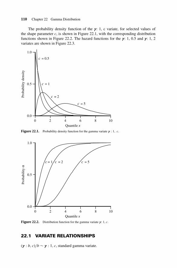
110 Chapter 22 Gamma Distribution
The probability density function of the γ: 1, c variate, for selected values ofthe shape parameter c, is shown in Figure 22.1, with the corresponding distributionfunctions shown in Figure 22.2. The hazard functions for the γ: 1, 0.5 and γ: 1, 2variates are shown in Figure 22.3.
Quantile x
Prob
abili
ty d
ensi
ty
0 642 1080.0
0.5
1.0
c = 0.5
c = 1
c = 2
c = 5
Figure 22.1. Probability density function for the gamma variate γ : 1, c.
Quantile x
Prob
abili
ty α
0 642 1080.0
0.5
1.0
c = 5 c = 2 c = 1
Figure 22.2. Distribution function for the gamma variate γ: 1, c.
22.1 VARIATE RELATIONSHIPS
(γ : b, c)/b ∼ γ : 1, c, standard gamma variate.
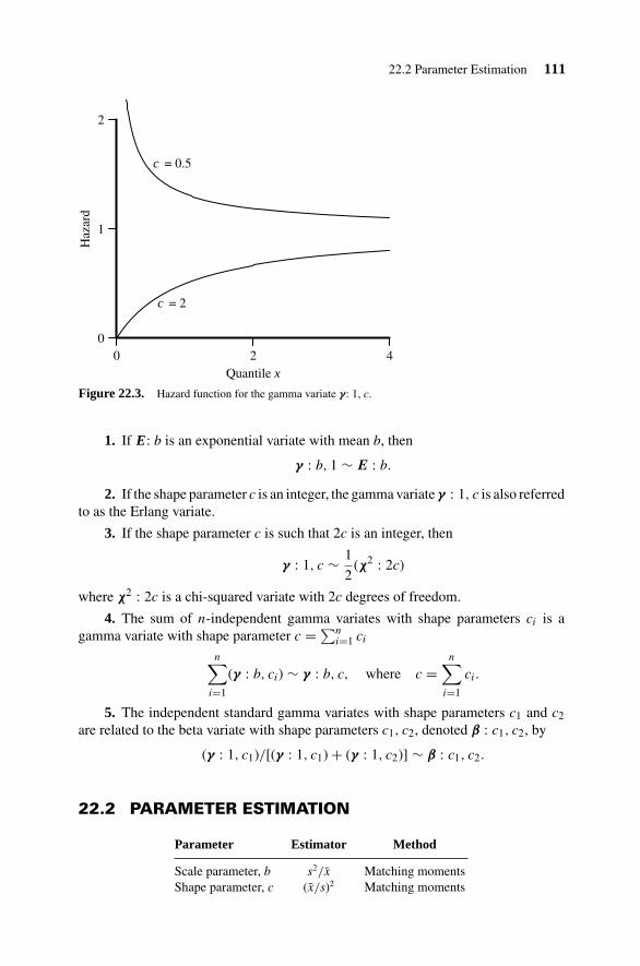
22.2 Parameter Estimation 111
Quantile x
Haz
ard
20 40
1
2
c = 0.5
c = 2
Figure 22.3. Hazard function for the gamma variate γ: 1, c.
1. If E: b is an exponential variate with mean b, then
γ : b, 1 ∼ E : b.
2. If the shape parameter c is an integer, the gamma variate γ : 1, c is also referredto as the Erlang variate.
3. If the shape parameter c is such that 2c is an integer, then
γ : 1, c ∼ 1
2(χ2 : 2c)
where χ2 : 2c is a chi-squared variate with 2c degrees of freedom.
4. The sum of n-independent gamma variates with shape parameters ci is agamma variate with shape parameter c = ∑n
i=1 ci
n∑i=1
(γ : b, ci) ∼ γ : b, c, where c =n∑
i=1
ci.
5. The independent standard gamma variates with shape parameters c1 and c2are related to the beta variate with shape parameters c1, c2, denoted β : c1, c2, by
(γ : 1, c1)/[(γ : 1, c1) + (γ : 1, c2)] ∼ β : c1, c2.
22.2 PARAMETER ESTIMATION
Parameter Estimator Method
Scale parameter, b s2/x Matching momentsShape parameter, c (x/s)2 Matching moments

112 Chapter 22 Gamma Distribution
Maximum-likelihood estimators b and c are solutions of the simultaneous equations[see Section 8.1 for ψ(c)].
b = x/c
log c − ψ(c) = log
⎡⎣x
/ (n∏
i=1
xi
)1/n⎤⎦ .
22.3 RANDOM NUMBER GENERATION
Variates γ: b, c for the case where c is an integer (equivalent to the Erlang variate)can be computed using
γ : b, c ∼ −b log
(c∏
i=1
Ri
)=
c∑i=1
−b log Ri.
where the Ri are independent unit rectangular variates.
22.4 INVERTED GAMMA DISTRIBUTION
The variate 1/(γ : λ = 1/b, c) is the inverted gamma variate and has probabilitydensity function (with quantile y)
exp(−λ/y)λc(1/y)c+1
�(c).
Its mean is λ/(c − 1) for c > 1 and its variance is
λ2/[(c − 1)2(c − 2)] for c > 2.
22.5 NORMAL GAMMA DISTRIBUTION
For a normal N : μ, σ variate, the normal gamma prior density for (μ, σ) is obtainedby specifying a normal density for the conditional prior of μ given σ, and an invertedgamma density for the marginal prior of σ, and is
τ1/2
(2π)1/2σexp
(− τ
2σ2 (μ − μ0)2)
× 2
�(ν/2)
(νs2
2
)ω/21
σν+1 exp
(− νs2
2σ2
)
where μ0, τ, ν, and s2 are the parameters of the prior distribution. In particular,
E(μ|σ) = E(μ) = μ0, variance (μ|σ) = σ2/τ.
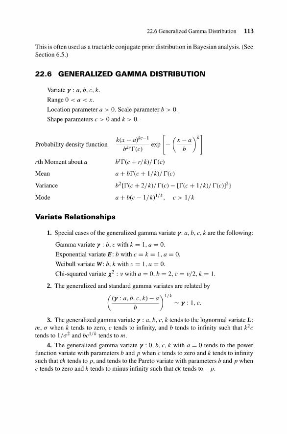
22.6 Generalized Gamma Distribution 113
This is often used as a tractable conjugate prior distribution in Bayesian analysis. (SeeSection 6.5.)
22.6 GENERALIZED GAMMA DISTRIBUTION
Variate γ : a, b, c, k.
Range 0 < a < x.
Location parameter a > 0. Scale parameter b > 0.
Shape parameters c > 0 and k > 0.
Probability density functionk(x − a)kc−1
bkc�(c)exp
[−
(x − a
b
)k]
rth Moment about a br�(c + r/k)/�(c)
Mean a + b�(c + 1/k)/�(c)
Variance b2{�(c + 2/k)/�(c) − [�(c + 1/k)/�(c)]2}Mode a + b(c − 1/k)1/k, c > 1/k
Variate Relationships
1. Special cases of the generalized gamma variate γ: a, b, c, k are the following:
Gamma variate γ : b, c with k = 1, a = 0.
Exponential variate E: b with c = k = 1, a = 0.
Weibull variate W: b, k with c = 1, a = 0.
Chi-squared variate χ2 : ν with a = 0, b = 2, c = ν/2, k = 1.
2. The generalized and standard gamma variates are related by((γ : a, b, c, k) − a
b
)1/k
∼ γ : 1, c.
3. The generalized gamma variate γ : a, b, c, k tends to the lognormal variate L:m, σ when k tends to zero, c tends to infinity, and b tends to infinity such that k2c
tends to 1/σ2 and bc1/k tends to m.
4. The generalized gamma variate γ : 0, b, c, k with a = 0 tends to the powerfunction variate with parameters b and p when c tends to zero and k tends to infinitysuch that ck tends to p, and tends to the Pareto variate with parameters b and p whenc tends to zero and k tends to minus infinity such that ck tends to −p.
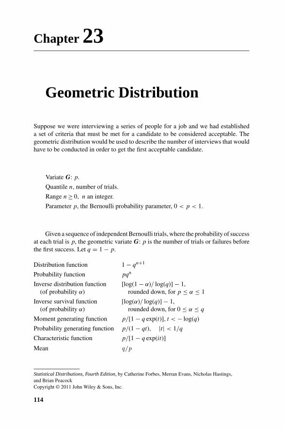
Chapter 23
Geometric Distribution
Suppose we were interviewing a series of people for a job and we had establisheda set of criteria that must be met for a candidate to be considered acceptable. Thegeometric distribution would be used to describe the number of interviews that wouldhave to be conducted in order to get the first acceptable candidate.
Variate G: p.
Quantile n, number of trials.
Range n ≥ 0, n an integer.
Parameter p, the Bernoulli probability parameter, 0 < p < 1.
Given a sequence of independent Bernoulli trials, where the probability of successat each trial is p, the geometric variate G: p is the number of trials or failures beforethe first success. Let q = 1 − p.
Distribution function 1 − qn+1
Probability function pqn
Inverse distribution function [log(1 − α)/ log(q)] − 1,(of probability α) rounded down, for p ≤ α ≤ 1
Inverse survival function [log(α)/ log(q)] − 1,(of probability α) rounded down, for 0 ≤ α ≤ q
Moment generating function p/[1 − q exp(t)], t < − log(q)
Probability generating function p/(1 − qt), |t| < 1/q
Characteristic function p/[1 − q exp(it)]
Mean q/p
Statistical Distributions, Fourth Edition, by Catherine Forbes, Merran Evans, Nicholas Hastings,and Brian PeacockCopyright © 2011 John Wiley & Sons, Inc.
114

23.2 Variate Relationships 115
Quantile n, number of trials
Prob
abili
ty
0.0
0.1
0.2
0.3
0.4
0.5
86420
p = 0.25
Quantile n, number of trials
Prob
abili
ty
0.0
0.1
0.2
0.3
0.4
0.5
6420
p = 0.5
Figure 23.1. Probability function for the geometric variate G: p.
Moments about mean
Variance q/p2
Third q(1 + q)/p3
Fourth (9q2/p4) + (q/p2)
Mode 0
Coefficient of skewness (1 + q)/q1/2
Coefficient of kurtosis 9 + p2/q
Coefficient of variation q−1/2
23.1 NOTES
1. The geometric distribution is a discrete analogue of the continuous exponentialdistribution and only these are characterized by a “lack of memory.”
2. An alternative form of the geometric distribution involves the number of trialsup to and including the first success. This has probability function pqn−1, mean 1/p,and probability generating function pt/(1 − qt). The geometric distribution is alsosometimes called the Pascal distribution.
The probability functions for the G: 0.25 and G: 0.5 variates are shown in thetwo panels of Figure 23.1.
23.2 VARIATE RELATIONSHIPS
1. The geometric variate is a special case of the negative binomial variate NB:x, p with x = 1.
G : p ∼ NB : 1, p.

116 Chapter 23 Geometric Distribution
2. The sum of x-independent geometric variates is the negative binomial variate
x∑i=1
(G : p)i ∼ NB : x, p.
23.3 RANDOM NUMBER GENERATION
Random numbers of the geometric variate G: p can be generated from random num-bers of the unit rectangular variate R using the relationship
G : p ∼ [log(R)/ log(1 − p)] − 1
rounded up to the next larger integer.

Chapter 24
Hypergeometric Distribution
Suppose a wildlife biologist is interested in the reproductive success of wolves thathad been introduced into an area. Her approach could be to catch a sample, size X,and place radio collars on them. The next year, after the wolf packs had been allowedto spread, a second sample, size n, could be caught and the number of this sample thathad the radio collars would be x. The hypergeometric distribution could then be usedto estimate the total number of wolves, N, in the area. This example illustrates animportant point in the application of theory to practice—that is, the assumptions thatmust be made to make the application of a particular theory (distribution) reliable andvalid. In the cited example it was assumed that the wolves had intermixed randomlyand that the samples were drawn randomly and independently on the successiveyears. Also, it was assumed that there had been minimal losses due to the activitiesof hunters or farmers or gains due to reproduction or encroachment from other areas.Probability and statistical distribution theory provide useful research tools, whichmust be complemented by domain knowledge.
Variate H : N, X, n.
Quantile x, number of successes.
Range max[0, n − N + X] ≤ x ≤ min[X, n].
Parameters N, the number of elements in the population; X, the number ofsuccesses in the population; n, sample size.
From a population of N elements of which X are successes (i.e., possess a certainattribute) we draw a sample of n items without replacement. The number of successesin such a sample is a hypergeometric variate H : N, X, n.
Probability function(probability of exactly x successes)
(X
x
) (N − X
n − x
) / (N
n
)
Mean nX/N
Moments about the meanVariance (nX/N)(1 − X/N)(N − n)/(N − 1)
Statistical Distributions, Fourth Edition, by Catherine Forbes, Merran Evans, Nicholas Hastings,and Brian PeacockCopyright © 2011 John Wiley & Sons, Inc.
117
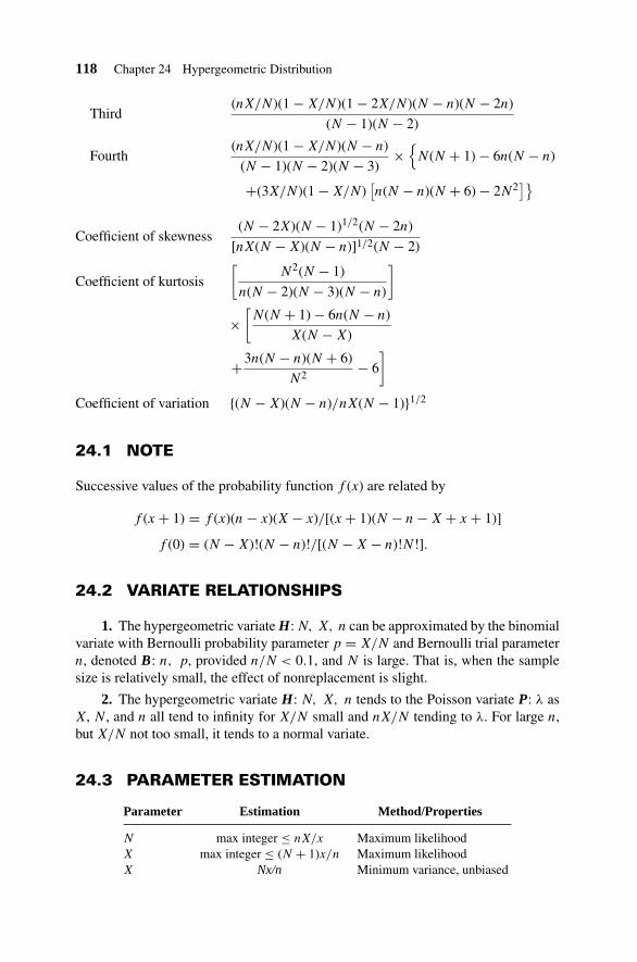
118 Chapter 24 Hypergeometric Distribution
Third(nX/N)(1 − X/N)(1 − 2X/N)(N − n)(N − 2n)
(N − 1)(N − 2)
Fourth(nX/N)(1 − X/N)(N − n)
(N − 1)(N − 2)(N − 3)×
{N(N + 1) − 6n(N − n)
+(3X/N)(1 − X/N)[n(N − n)(N + 6) − 2N2
]}
Coefficient of skewness(N − 2X)(N − 1)1/2(N − 2n)
[nX(N − X)(N − n)]1/2(N − 2)
Coefficient of kurtosis
[N2(N − 1)
n(N − 2)(N − 3)(N − n)
]
×[N(N + 1) − 6n(N − n)
X(N − X)
+3n(N − n)(N + 6)
N2 − 6
]
Coefficient of variation {(N − X)(N − n)/nX(N − 1)}1/2
24.1 NOTE
Successive values of the probability function f (x) are related by
f (x + 1) = f (x)(n − x)(X − x)/[(x + 1)(N − n − X + x + 1)]
f (0) = (N − X)!(N − n)!/[(N − X − n)!N!].
24.2 VARIATE RELATIONSHIPS
1. The hypergeometric variate H: N, X, n can be approximated by the binomialvariate with Bernoulli probability parameter p = X/N and Bernoulli trial parametern, denoted B: n, p, provided n/N < 0.1, and N is large. That is, when the samplesize is relatively small, the effect of nonreplacement is slight.
2. The hypergeometric variate H: N, X, n tends to the Poisson variate P: λ asX, N, and n all tend to infinity for X/N small and nX/N tending to λ. For large n,but X/N not too small, it tends to a normal variate.
24.3 PARAMETER ESTIMATION
Parameter Estimation Method/Properties
N max integer ≤ nX/x Maximum likelihoodX max integer ≤ (N + 1)x/n Maximum likelihoodX Nx/n Minimum variance, unbiased
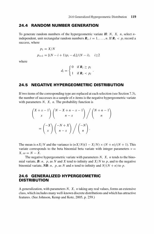
24.6 Generalized Hypergeometric Distribution 119
24.4 RANDOM NUMBER GENERATION
To generate random numbers of the hypergeometric variate H: N, X, n, select n-independent, unit rectangular random numbers Ri, i = 1, . . . , n. If Ri < pi record asuccess, where
p1 = X/N
pi+1 = [(N − i + 1)pi − di]/(N − i), i≥2
where
di ={
0 if Ri ≥ pi
1 if Ri < pi
.
24.5 NEGATIVE HYPERGEOMETRIC DISTRIBUTION
If two items of the corresponding type are replaced at each selection (see Section 7.3),the number of successes in a sample of n items is the negative hypergeometric variatewith parameters N, X, n. The probability function is
(X + x − 1
x
) (N − X + n − x − 1
n − x
) / (N + n − 1
n
)
=(−X
x
) (−N + X
n − x
) / (−N
n
).
The mean is nX/N and the variance is (nX/N)(1 − X/N) × (N + n)/(N + 1). Thisvariate corresponds to the beta binomial beta variate with integer parameters ν =X, ω = N − X.
The negative hypergeometric variate with parameters N, X, n tends to the bino-mial variate, B: n, p, as N and X tend to infinity and X/N to p, and to the negativebinomial variate, NB: n, p, as N and n tend to infinity and N/(N + n) to p.
24.6 GENERALIZED HYPERGEOMETRICDISTRIBUTION
A generalization, with parameters N, X, n taking any real values, forms an extensiveclass, which includes many well-known discrete distributions and which has attractivefeatures. (See Johnson, Kemp and Kotz, 2005, p. 259.)

Chapter 25
Inverse Gaussian (Wald)Distribution
The inverse Gaussian distribution has applications in the study of diffusion processesand as a lifetime distribution model.
Variate I: μ, λ.
Range x > 0.
Location parameter μ > 0, the mean.
Scale parameter λ > 0.
Probability density function(λ/(2πx3)
)1/2exp
(−λ(x − μ)2
2μ2x
)
Moment generating function exp
{λ
μ
[1 −
(1 − 2μ2t
λ
)1/2]}
Characteristic function exp
{λ
μ
[1 −
(1 − 2μ2it
λ
)1/2]}
rth Cumulant 1 · 3 · 5 · · · (2r − 3)μ2r−1λ1−r, r ≥ 2
Cumulant generating functionλ
μ
[1 −
(1 + 2
μ2it
λ
)1/2]
rth Moment about the origin μrr−1∑i=0
(r − 1 + i)!
i!(r − 1 − i)!
( μ
2λ
)i
, r ≥ 2
Mean μ
Variance μ3/λ
Statistical Distributions, Fourth Edition, by Catherine Forbes, Merran Evans, Nicholas Hastings,and Brian PeacockCopyright © 2011 John Wiley & Sons, Inc.
120

25.2 Parameter Estimation 121
Quantile x
Prob
abili
ty d
ensi
ty
0.0 0.5 1.0 1.5 2.0 2.5 3.00.0
0.5
1.0
1.5
2.0
2.5
λ = 0.5
λ = 0.25
λ = 1
λ = 2
μ = 1
Figure 25.1. Probability density function for the inverse Gaussian variate I: μ, λ.
Mode μ
[(1 + 9μ2
4λ2
)1/2
− 3μ
2λ
]
Coefficient of skewness 3(μ/λ)1/2
Coefficient of kurtosis 3 + 15μ/λ
Coefficient of variation (μ/λ)1/2
The probability density function for the I: 1, λ variate is shown in Figure 25.1for selected values of the scale parameter λ.
25.1 VARIATE RELATIONSHIPS
1. The standard Wald variate is a special case of the inverse Gaussian variate I:μ, λ, for μ = 1.
2. The standard inverse Gaussian variate I: μ, λ tends to the standard normalvariate N: 0, 1 as λ tends to infinity.
25.2 PARAMETER ESTIMATION
Parameter Estimator Method/Properties
μ x Maximum likelihood
λ n
/(n∑
i=1
x−1i − (x)−1
)Maximum likelihood
λ (n − 1)
/(n∑
i=1
x−1i − (x)−1
)Minimum variance,unbiased
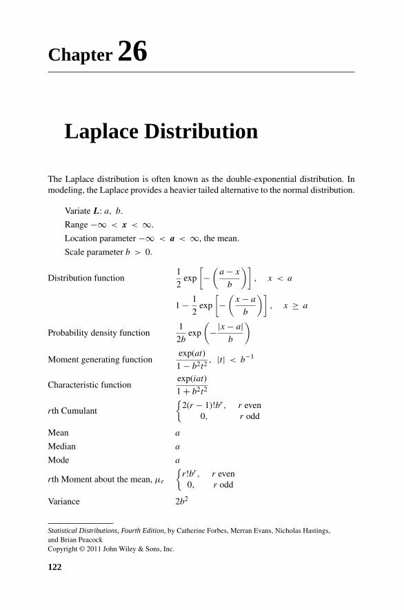
Chapter 26
Laplace Distribution
The Laplace distribution is often known as the double-exponential distribution. Inmodeling, the Laplace provides a heavier tailed alternative to the normal distribution.
Variate L: a, b.
Range −∞ < x < ∞.
Location parameter −∞ < a < ∞, the mean.
Scale parameter b > 0.
Distribution function1
2exp
[−
(a − x
b
)], x < a
1 − 1
2exp
[−
(x − a
b
)], x ≥ a
Probability density function1
2bexp
(−|x − a|
b
)
Moment generating functionexp(at)
1 − b2t2 , |t| < b−1
Characteristic functionexp(iat)
1 + b2t2
rth Cumulant
{2(r − 1)!br, r even
0, r odd
Mean a
Median a
Mode a
rth Moment about the mean, μr
{r!br, r even
0, r odd
Variance 2b2
Statistical Distributions, Fourth Edition, by Catherine Forbes, Merran Evans, Nicholas Hastings,and Brian PeacockCopyright © 2011 John Wiley & Sons, Inc.
122
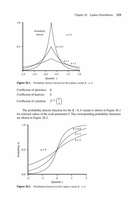
Chapter 26 Laplace Distribution 123
Quantile x
0.5
1.0
−2.5 −1.5 −0.5 0.5 1.5 2.5
b = 0.5
b = 1 b = 2
a = 0
Probabilitydensity
Figure 26.1. Probability density function for the Laplace variate L : a, b.
Coefficient of skewness 0
Coefficient of kurtosis 6
Coefficient of variation 21/2(
b
a
)
The probability density function for the L : 0, b variate is shown in Figure 26.1for selected values of the scale parameter b. The corresponding probability functionsare shown in Figure 26.2.
Quantile x
Prob
abili
ty α
0.0
0.5
1.0
−2 −1 10 2
b = 0.5
b = 1
b = 2
a = 0
Figure 26.2. Distribution function for the Laplace variate L : a, b.

124 Chapter 26 Laplace Distribution
26.1 VARIATE RELATIONSHIPS
1. The Laplace variate L: a, b is related to the independent exponential variatesE: b and E: 1 by
E : b ∼ |(L : a, b) − a|E : 1 ∼ |(L : a, b) − a|/b.
2. The Laplace variate L: 0, b is related to two independent exponential variatesE: b by
L : 0, b ∼ (E : b)1 − (E : b)2.
3. Two independent Laplace variates, with parameter a = 0, are related to the Fvariate with parameters ν = ω = 2, F: 2, 2, by
F : 2, 2 ∼ |(L : 0, b)1/(L : 0, 2)2|.
26.2 PARAMETER ESTIMATION
Parameter Estimator Method/Properties
a Median Maximum likelihood
b 1n
n∑i=1
|xi − a| Maximum likelihood
26.3 RANDOM NUMBER GENERATION
The standard Laplace variate L: 0, 1 is related to the independent unit rectangularvariates R1, R2 by
L : 0, 1 ∼ log(R1/R2).

Chapter 27
Logarithmic SeriesDistribution
Range x ≥ 1, an integer.
Shape parameter 0 < c < 1.
For simplicity, also let k = −1/ log(1 − c).
Probability function kcx/x
Probability generating function log(1 − ct)/ log(1 − c), |t| < 1/c
Moment generating function log[1 − c exp(t)]/ log(1 − c)
Characteristic function log[1 − c exp(it)]/ log(1 − c)
Moments about the origin
Mean kc(1 − c)
Second kc/(1 − c)2
Third kc(1 + c)/(1 − c)3
Fourth kc(1 + 4c + c2)/(1 − c)4
Moments about the meanVariance kc(1 − kc)/(1 − c)2
Third kc(1 + c − 3kc + 2k2c2)/(1 − c)3
Fourthkc[1 + 4c + c2 − 4kc(1 + c) + 6k2c2 − 3k3c3]
(1 − c)4
Coefficient of skewness(1 + c) − 3kc + 2k2c2
(kc)1/2(1 − kc)3/2
Coefficient of kurtosis1 + 4c + c2 − 4kc(1 + c) + 6k2c2 − 3k3c3
kc(1 − kc)2
Statistical Distributions, Fourth Edition, by Catherine Forbes, Merran Evans, Nicholas Hastings,and Brian PeacockCopyright © 2011 John Wiley & Sons, Inc.
125

126 Chapter 27 Logarithmic Series Distribution
Quantile x
Prob
abili
ty α
0.0
0.1
0.2
0.3
0.4
0.5
0.6
0.7
0.8
42
c = 0.5
Quantile xPr
obab
ility
α
0.0
0.1
0.2
0.3
0.4
155 25
c = 0.9
Figure 27.1. Probability function for the logarithmic series variate.
The probability functions for the logarithmic series variate, with shape parametersc = 0.5 and c = 0.9 are shown in the two panels of Figure 27.1.
27.1 VARIATE RELATIONSHIPS
1. The logarithmic series variate with parameter c corresponds to the powerseries distribution variate with parameter c and series function − log(1 − c).
2. The limit toward zero of a zero truncated (i.e., excluding x = 0) negative bi-nomial variate with parameters x and p = 1 − c is a logarithmic series variatewith parameter c.
27.2 PARAMETER ESTIMATION
The maximum-likelihood and method of moments estimators c satisfy the equation
x = c
−(1 − c) log(1 − c).
Other asymptotically unbiased estimators of c are
1 −(
proportion of
x′s equal to 1
)/x
1 −(n−1
∑x2j
) /x.

Chapter 28
Logistic Distribution
The distribution function of the logistic is used as a model for growth. For example,with a new product we often find that growth is initially slow, then gains momentum,and finally slows down when the market is saturated or some form of equilibrium isreached.
Applications include the following:
• Market penetration of a new product
• Population growth
• The expansion of agricultural production
• Weight gain in animals
Range −∞ < x < ∞.
Location parameter a, the mean.
Scale parameter b > 0.
Alternative parameter k = πb/31/2, the standard deviation.
Distribution function 1 − {1 + exp[(x − a)/b]}−1
= {1 + exp[−(x − a)/b]}−1
= 1
2
{1 + tanh
[1
2(x − a)/b
]}
Probability density functionexp[−(x − a)/b]
b{1 + exp[−(x − a)/b]}2
= exp[(x − a)/b]
b{1 + exp[(x − a)/b]}2
= sech2[(x − a)/2b]
4b
Statistical Distributions, Fourth Edition, by Catherine Forbes, Merran Evans, Nicholas Hastings,and Brian PeacockCopyright © 2011 John Wiley & Sons, Inc.
127

128 Chapter 28 Logistic Distribution
Inverse distribution function a + b log[α/(1 − α)](of probability α)
Survival function {1 + exp[(x − a)/b]}−1
Inverse survival function a + b log[(1 − α)/α](of probability α)
Hazard function {b{1 + exp[−(x − a)/b]}}−1
Cumulative hazard function log{1 + exp[(x − a)/b]}Moment generating function exp(at)�(1 − bt)�(1 + bt) = πbt exp(at)/ sin(πbt)
Characteristic function exp(iat)πbit/ sin(πbit)
Mean a
Variance π2b2/3
Mode a
Median a
Coefficient of skewness 0
Coefficient of kurtosis 4.2
Coefficient of variation πb/(31/2a)
28.1 NOTES
1. The logistic distribution is the limiting distribution, as n tends to infinity, ofthe average of the largest to smallest sample values, of random samples ofsize n from an exponential-type distribution.
2. The standard logistic variate, here denoted X: 0, 1 with parameters a = 0, b =1, has a distribution function FX and probability density function fX with theproperties
fX = FX(1 − FX)
x = log[FX/(1 − FX)].
The probability density function for the logistic variate is shown in Figure 28.1for location parameter a = 0 and for selected values of the scale parameter b. Thecorresponding probability functions are shown in Figure 28.2.
28.2 VARIATE RELATIONSHIPS
The standard logistic variate, here denoted X: 0, 1, is related to the logistic variate,denoted X: a, b by
X : 0, 1 ∼ [(X : a, b) − a]/b.

28.2 Variate Relationships 129
Quantile x
−4 −3 −2 −1 43210
0.2
0.4
0.6
Probabilitydensity
b = 0.5
b = 1
b = 2
a = 0
Figure 28.1. Probability density function for the logistic variate.
Quantile x
−4 −3 −2 −1 43210
0.5
1.0
Probabilityα
b = 0.5
b = 1
b = 2
a = 0
Figure 28.2. Distribution function for the logistic variate.
1. The standard logistic variate X: 0, 1 is related to the standard exponentialvariate E: 1 by
X : 0, 1 ∼ − log{exp(−E : 1)/[1 + exp(−E : 1)]}.

130 Chapter 28 Logistic Distribution
For two independent standard exponential variates E: 1, then
X : 0, 1 ∼ − log[(E : 1)1/(E : 1)2].
2. The standard logistic variate X: 0, 1 is the limiting form of the weighted sumof n-independent standard Gumbel extreme value variates V: 0, 1 as n tends to infinity
X : 0, 1 ≈n∑
i=1
(V : 0, 1)i/ i, n → ∞.
3. Two independent standard Gumbel extreme value variates, V: a, b, are relatedto the logistic variate X: 0, b by
X : 0, b ∼ (V : a, b)1 − (V : a, b)2.
4. The Pareto variate, here denoted Y: a, c, is related to the standard logisticvariate X: 0, 1 by
X : 0, 1 ∼ − log{[(Y : a, c)/a]c − 1}.5. The standard power function variate, here denoted Y: 1, c, is related to the
standard logistic variate X: 0, 1 by
X : 0, 1 ∼ − log[(Y : 1, c)−c − 1].
28.3 PARAMETER ESTIMATION
The maximum-likelihood estimators a and b of the location and scale parameters arethe solutions of the simultaneous equations
n
2=
n∑i=1
exp(
xi−a
b
)[1 + exp
(xi−a
b
)]
n =n∑
i=1
(xi − a
b
) exp(
xi−a
b
)− 1
exp(
xi−a
b
)+ 1
.
28.4 RANDOM NUMBER GENERATION
Let R denote a unit rectangular variate. Random numbers of the logistic variate X: a,b can be generated using the relation
X : a, b ∼ a + b log[R/(1 − R)].

Chapter 29
Lognormal Distribution
The lognormal distribution is applicable to random variables that are constrained byzero but have a few very large values. The resulting distribution is asymmetrical andpositively skewed. Examples include the following:
• The weight of adults
• The concentration of minerals in deposits
• Duration of time off due to sickness
• Distribution of wealth
• Machine down times
The application of a logarithmic transformation to the data can allow the datato be approximated by the symmetrical normal distribution, although the absence ofnegative values may limit the validity of this procedure.
Variate L : m, σ or L : μ, σ.
Range 0 ≤ x < ∞.
Scale parameter m > 0, the median.
Alternative parameter μ, the mean of log L.
m and μ are related by m = exp μ, μ = log m.
Shape parameter σ > 0, the standard deviation of log L.
For compactness the substitution ω = exp(σ2) is used in several formulas.
Probability density function1
xσ(2π)1/2 exp
(−[log(x/m)]2
2σ2
)
= 1
xσ(2π)1/2 exp
(−(log x − μ)2
2σ2
)
Statistical Distributions, Fourth Edition, by Catherine Forbes, Merran Evans, Nicholas Hastings,and Brian PeacockCopyright © 2011 John Wiley & Sons, Inc.
131
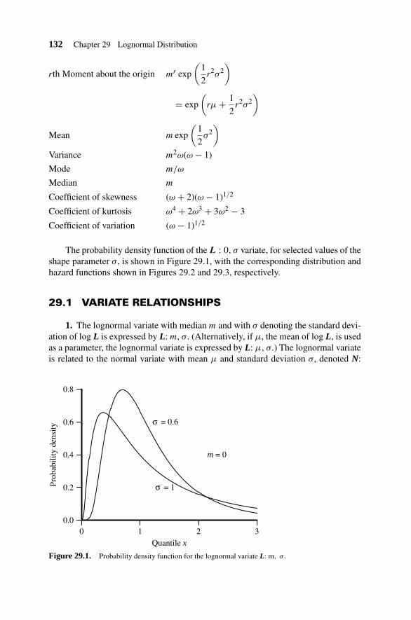
132 Chapter 29 Lognormal Distribution
rth Moment about the origin mr exp
(1
2r2σ2
)
= exp
(rμ + 1
2r2σ2
)
Mean m exp
(1
2σ2
)
Variance m2ω(ω − 1)
Mode m/ω
Median m
Coefficient of skewness (ω + 2)(ω − 1)1/2
Coefficient of kurtosis ω4 + 2ω3 + 3ω2 − 3
Coefficient of variation (ω − 1)1/2
The probability density function of the L : 0, σ variate, for selected values of theshape parameter σ, is shown in Figure 29.1, with the corresponding distribution andhazard functions shown in Figures 29.2 and 29.3, respectively.
29.1 VARIATE RELATIONSHIPS
1. The lognormal variate with median m and with σ denoting the standard devi-ation of log L is expressed by L: m, σ. (Alternatively, if μ, the mean of log L, is usedas a parameter, the lognormal variate is expressed by L: μ, σ.) The lognormal variateis related to the normal variate with mean μ and standard deviation σ, denoted N:
Quantile x
Prob
abili
ty d
ensi
ty
210 30.0
0.2
0.4
0.6
0.8
σ = 0.6
σ = 1
m = 0
Figure 29.1. Probability density function for the lognormal variate L: m, σ.
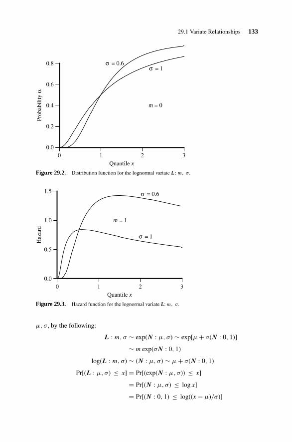
29.1 Variate Relationships 133
Quantile x
Prob
abili
ty α
210 30.0
0.2
0.4
0.6
0.8 σ = 0.6 σ = 1
m = 0
Figure 29.2. Distribution function for the lognormal variate L : m, σ.
Quantile x
Haz
ard
210 30.0
0.5
1.0
1.5 σ = 0.6
σ = 1
m = 1
Figure 29.3. Hazard function for the lognormal variate L: m, σ.
μ, σ, by the following:
L : m, σ ∼ exp(N : μ, σ) ∼ exp[μ + σ(N : 0, 1)]
∼ m exp(σN : 0, 1)
log(L : m, σ) ∼ (N : μ, σ) ∼ μ + σ(N : 0, 1)
Pr[(L : μ, σ) ≤ x] = Pr[(exp(N : μ, σ)) ≤ x]
= Pr[(N : μ, σ) ≤ log x]
= Pr[(N : 0, 1) ≤ log((x − μ)/σ)]

134 Chapter 29 Lognormal Distribution
2. For small σ, the normal variate N : log μ, σ approximates the lognormal vari-ate L : μ, σ.
3. Transformations of the following form, for a and b constant, of the lognormalvariate L : μ, σ are also lognormal:
exp(a)(L : μ, σ)b ∼ L : a + bμ, bσ.
4. For two independent lognormal variates, L : μ1, σ1 and L : μ2, σ2,
(L : μ1, σ1) × (L : μ2, σ2) ∼ L : μ1 + μ2, (σ21 + σ2
2 )1/2
(L : μ1, σ1)/(L : μ2, σ2) ∼ L : μ1 − μ2, (σ21 + σ2
2 )1/2.
5. The geometric mean of the n-independent lognormal variates L : μ, σ is alsoa lognormal variate (
n∏i=1
(L : μ, σ)i
)1/n
∼ L : μ, σ/n1/2.
29.2 PARAMETER ESTIMATION
The following estimators are derived by transformation to the normal distribution.
Parameter Estimator
Median, m m = exp μ
Mean of log(L), μ μ =(
1
n
)n∑
i=1log xi
Variance of log(L), σ2 σ2 =(
1
n − 1
)n∑
i=1[log(xi − μ)]2
29.3 RANDOM NUMBER GENERATION
The relationship of the lognormal variate L : m, σ to the unit normal variate N: 0,1 gives
L : m, σ ∼ m exp(σN : 0, 1)
∼ exp[μ + σ(N : 0, 1)].

Chapter 30
Multinomial Distribution
The multinomial variate is a multidimensional generalization of the binomial. Con-sider a trial that can result in only one of k possible distinct outcomes, labeledAi, i = 1, . . . , k. Outcome Ai occurs with probability pi. The multinomial distri-bution relates to a set of n-independent trials of this type. The multinomial multi-variate is M = [Mi], where Mi is the variate “number of times event Ai occurs,”i = 1, . . . , k. The quantile is a vector x = [x1, . . . , xk]′. For the multinomial variate,xi is the quantile of Mi and is the number of times event Ai occurs in the n trials.
Suppose we wish to test the robustness of a complex component of an automobileunder crash conditions. The component may be damaged in various ways each withdifferent probabilities. If we wish to evaluate the probability of a particular combina-tion of failures we could apply the multinomial distribution. A useful approximationto the multinomial distribution is the application of the chi-squared distribution to theanalysis of contingency tables.
Multivariate M : n, p1, . . . , pk.
Range xi ≥ 0,∑k
i=1 xi = n, xi an integer.
Parameters n and pi, i = 1, . . . , k, where 0 < pi < 1,∑k
i=1 pi = 1.
The joint probability function f (x1, . . . , xk) is the probability that each event Ai
occurs xi times, i = 1, . . . , k, in the n trials, and is given by
Probability function n!k∏
i=1(pxi
i /xi!)
Probability generating function
(k∑
i=1piti
)n
Moment generating function
(k∑
i=1pi exp(ti)
)n
Cumulant generating function n log
(k∑
i=1pi exp(iti)
)
Statistical Distributions, Fourth Edition, by Catherine Forbes, Merran Evans, Nicholas Hastings,and Brian PeacockCopyright © 2011 John Wiley & Sons, Inc.
135

136 Chapter 30 Multinomial Distribution
Individual elements, Mi
Mean npi
Variance npi(1 − pi)
Covariance −npipj, i /= j
Third cumulant
⎧⎨⎩
npi(1 − pi)(1 − 2pi) i = j = k
−npipk(1 − 2pi) i = j /= k
2npipjpk i, j, k all distinct
Fourth cumulant
⎧⎪⎪⎪⎪⎨⎪⎪⎪⎪⎩
npi(1 − pi)[1 − 6pi(1 − pi)
]i = j = k = l
−npipl
[1 − 6pi(1 − pi)
]i = j = k /= l
−npipk[1 − 2pi − 2pk + 6pipk] i = j /= k = l
2npipkpl(1 − 3pi) i = j /= k /= l
−6npipjpkpl i, j, k, l all distinct
30.1 VARIATE RELATIONSHIPS
If k = 2 and p1 = p, the multinomial variate corresponds to the binomial variate B: n,p. The marginal distribution of each Mi is the binomial distribution with parametersn, pi.
30.2 PARAMETER ESTIMATION
For individual elements
Parameter Estimator Method/Properties
pi xi/n Maximum likelihood

Chapter 31
Multivariate Normal(Multinormal) Distribution
A multivariate normal distribution is a multivariate extension of the normal distribu-tion.
The bivariate normal distribution may be applied to the description of correlatedvariables, such as smoking and performance on respiratory function tests. An ex-tension of the concept may be applied to multiple correlated variables such as heartdisease, body weight, exercise, and dietary habits.
Multivariate MN : μ, �.
Quantile x = [x1, . . . , xk]′ a k×1 vector.
Range −∞ < xi < ∞, for i = 1, . . . , k.
Location parameter, the k×1 mean vector, μ = [μ1, . . . , μk]′, with −∞ <
μi < ∞.
Parameter �, the k × k positive definite variance-covariance matrix, withelements �ij = σij . Note σii = σ2
i .
Probability density function f (x) = (2π)−(1/2)k|�|−1/2
× exp[ − 1
2 (x − μ)′�−1(x − μ)]
Characteristic function exp( − 1
2 t′�t)
exp(it′μ
)Moment generating function exp
(μ′t + 1
2 t′�t)
Cumulant generating function − 12 t′�t + i′t′μ
Mean μ
Variance-covariance �
Moments about the mean
Third 0
Fourth σijσkl + σikσjl + σilσjk
Statistical Distributions, Fourth Edition, by Catherine Forbes, Merran Evans, Nicholas Hastings,and Brian PeacockCopyright © 2011 John Wiley & Sons, Inc.
137

138 Chapter 31 Multivariate Normal (Multinormal) Distribution
rth Cumulant 0 for r > 2For individual elements MN i
Probability density function (2π)−1/2|�ii|−1/2
× exp[ − 1
2
(xi − μi
)′�−1
ii
(xi − μi
)]Mean μi
Variance �ii = σ2i
Covariance �ij = σij
31.1 VARIATE RELATIONSHIPS
1. A fixed linear transformation of a multivariate normal variate is also a multi-variate normal variate. For a, a constant j×1 vector, and B, a j × k fixed matrix, theresulting variate is of dimension j×1:
a + B(MN : μ, �) ∼ (MN : a + Bμ, B�B′).
2. The multinormal variate with k = 1 corresponds to the normal variate N :μ, σ, where μ = μ1 and σ2 = �11.
3. The sample mean of variates with any joint distribution with finite meanand variance tends to the multivariate normal form. This is the simplest form of themultivariate central limit theorem.
31.2 PARAMETER ESTIMATION
For individual elements
Parameter Estimator Method/Properties
μi xi =n∑
t=1
xti Maximum likelihood
�ij
n∑t=1
(xti − xi)(xtj − xj) Maximum likelihood

Chapter 32
Negative Binomial Distribution
The Pascal variate is the number of failures before the xth success in a sequence ofBernoulli trials, where the probability of success at each trial is p and the probability offailure is q = 1 − p. This generalizes to the negative binomial variate for noninteger x.
Suppose prosecution and defense lawyers were choosing 12 citizens to comprisea jury. The Pascal distribution could be applied to estimate the number of rejectionsbefore the jury selection process was completed. The Pascal distribution is an ex-tension of the geometric distribution, which applies to the number of failures beforethe first success. The Pascal distribution generalizes to the negative binomial, whenthe definition of “success” is not an integer. An example of the negative binomialis the number of scoops of ice cream needed to fill a bowl, as this is not necessarilyan integer.
Variate NB: x, p.
Quantile y.
Range 0 ≤ y < ∞, y an integer.
Parameters 0 < x < ∞, 0 < p < 1, q = 1 − p.
Distribution function (Pascal)y∑
i=0
(x + i − 1
x − 1
)pxqi (integer x only)
Probability function (Pascal)
(x + y − 1
x − 1
)pxqy (integer x only)
Probability function �(x + y)pxqy/�(x)y!
Moment generating function px(1 − q exp t)−x, t < log(q)
Probability generating function px(1 − qt)−x, |t| < 1/q
Characteristic function px[1 − q exp(it)
]−x
Cumulant generating function x log(p) − x log[1 − q exp(it)
]
Statistical Distributions, Fourth Edition, by Catherine Forbes, Merran Evans, Nicholas Hastings,and Brian PeacockCopyright © 2011 John Wiley & Sons, Inc.
139
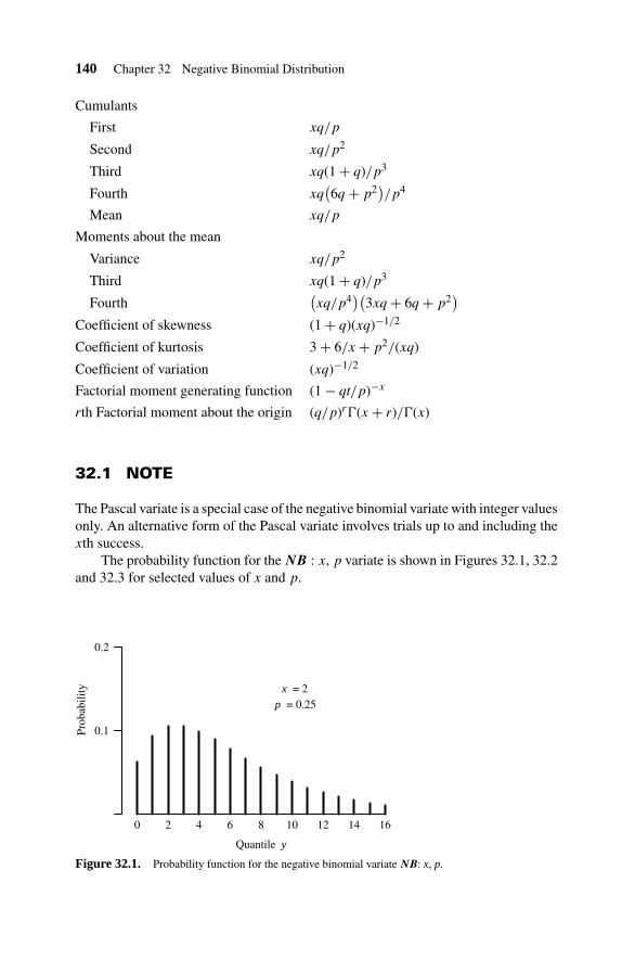
140 Chapter 32 Negative Binomial Distribution
Cumulants
First xq/p
Second xq/p2
Third xq(1 + q)/p3
Fourth xq(6q + p2
)/p4
Mean xq/p
Moments about the mean
Variance xq/p2
Third xq(1 + q)/p3
Fourth(xq/p4
)(3xq + 6q + p2
)Coefficient of skewness (1 + q)(xq)−1/2
Coefficient of kurtosis 3 + 6/x + p2/(xq)
Coefficient of variation (xq)−1/2
Factorial moment generating function (1 − qt/p)−x
rth Factorial moment about the origin (q/p)r�(x + r)/�(x)
32.1 NOTE
The Pascal variate is a special case of the negative binomial variate with integer valuesonly. An alternative form of the Pascal variate involves trials up to and including thexth success.
The probability function for the NB : x, p variate is shown in Figures 32.1, 32.2and 32.3 for selected values of x and p.
Quantile y
Prob
abili
ty
0.1
0.2
0 642 108 12 14 16
x = 2 p = 0.25
Figure 32.1. Probability function for the negative binomial variate NB: x, p.

32.2 Variate Relationships 141
Quantile y
Prob
abili
ty
0.1
0.2
0 642 108 12 14 16
x = 2
p = 0.5
Figure 32.2. Probability function for the negative binomial variate NB: x, p.
32.2 VARIATE RELATIONSHIPS
1. The sum of k-independent negative binomial variates NB: xi, p; i = 1, . . . , k
is a negative binomial variate NB: x′, p, where
k∑i = 1
(NB : xi, p) ∼ NB : x′, p, where x′ =k∑
i = 1
xi.
2. The geometric variate G: p is a special case of the negative binomial variatewith x = 1.
G : p ∼ NB : 1, p
Quantile y
Prob
abili
ty
0.1
0.2
0 642 108 12 14 16
x = 5
p = 0.5
Figure 32.3. Probability function for the negative binomial variate NB: x, p.
142 Chapter 32 Negative Binomial Distribution
3. The sum of x-independent geometric variates G: p is a negative binomialvariate.
x∑i = 1
(G : p)i ∼ NB : x, p
4. The negative binomial variate corresponds to the power series variate withparameter c = 1 − p, and probability function (1 − c)−x.
5. As x tends to infinity and p tends to 1 with x(1 − p) = λ held fixed, thenegative binomial variate tends to the Poisson variate, P : λ.
6. The binomial variate B: n, p and negative binomial variate NB: x, p arerelated by
Pr[(B : n, p) ≤ x
] = Pr[(NB : x, p) ≥ (n − x)
].
32.3 PARAMETER ESTIMATION
Parameter Estimator Method/Properties
p (x − 1)/(y + x − 1) Unbiased
p x/(y + x) Maximum likelihood
32.4 RANDOM NUMBER GENERATION
1. Rejection Technique. Select a sequence of unit rectangular random numbers,recording the numbers of those that are greater than and less than p. When the numberless than p first reaches x, the number greater than p is a negative binomial randomnumber, for x and y integer valued.
2. Geometric Distribution Method. If p is small, a faster method may be to addx geometric random numbers, as
NB : x, p ∼x∑
i=1
(G : p)i.
Chapter 33
Normal (Gaussian)Distribution
The normal distribution is applicable to a very wide range of phenomena and isthe most widely used distribution in statistics. It was originally developed as anapproximation to the binomial distribution when the number of trials is large andthe Bernoulli probability p is not close to 0 or 1. It is also the asymptotic form of thesum of random variables under a wide range of conditions.
The normal distribution was first described by the French mathematician deMoivre in 1733. The development of the distribution is often ascribed to Gauss, whoapplied the theory to the movements of heavenly bodies.
Variate N: μ, σ.
Range −∞ < x < ∞.
Location parameter μ, the mean.
Scale parameter σ > 0, the standard deviation.
Probability density function σ(2π)1/2/
exp
(−(x − μ)2
2σ2
)
Moment generating function exp
(μt + 1
2σ2t2
)
Characteristic function exp
(iμt − 1
2σ2t2
)
Cumulant generating
function iμt − 1
2σ2t2
rth Cumulant κ1 = μ, κ2 = σ2, κr = 0, r > 2
Mean μ
Statistical Distributions, Fourth Edition, by Catherine Forbes, Merran Evans, Nicholas Hastings,and Brian PeacockCopyright © 2011 John Wiley & Sons, Inc.
143

144 Chapter 33 Normal (Gaussian) Distribution
rth Moment about the mean
⎧⎨⎩
μr = 0 r oddμr = σrr!/{2r/2[(r/2)!]}
= σr(r − 1)(r − 3) · · · (3)(1) r even
Variance σ2
Mean deviation σ(2/π)1/2
Mode μ
Median μ
Standardized rth moment about themean
{ηr = 0 r oddηr = r!/{2r/2[(r/2)!]} r even
Coefficient of skewness 0
Coefficient of kurtosis 3
Information content log2[σ(2πe)1/2]
The probability density function of the standard N : 0, 1 variate is shown inFigure 33.1, with the corresponding distribution and hazard functions shown inFigure 33.2 and 33.3, respectively.
33.1 VARIATE RELATIONSHIPS
The standard normal variate N: 0, 1 and the normal variate N: μ, σ are related by
N : 0, 1 ∼ [(N : μ, σ) − μ]/σ.
1. Let N i, i = 1, . . . , n be independent normal variates with means μi andvariances σ2
i . Then∑n
i=1 ciN i is normally distributed with mean∑n
i=1 ciμi andvariance
∑ni=1 c2
i σ2i , where the ci, i = 1, . . . , n are constant weighting factors.
Quantile x
Prob
abili
ty d
ensi
ty
−3 −2 −1 3210
0.2
0.4
Figure 33.1. Probability density function for the standard normal variate N: 0, 1.
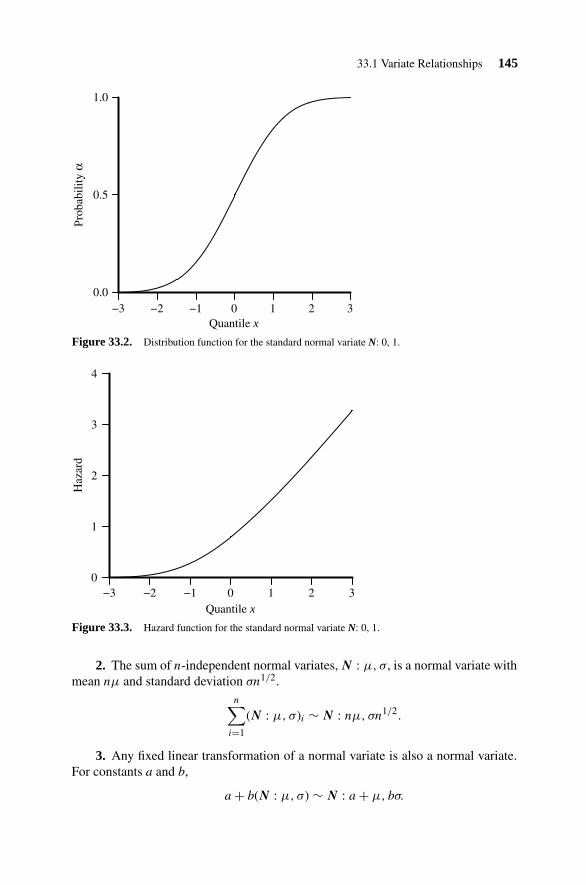
33.1 Variate Relationships 145
Quantile x
Prob
abili
ty α
−3 −2 −1 32100.0
0.5
1.0
Figure 33.2. Distribution function for the standard normal variate N: 0, 1.
Quantile x
Haz
ard
−3 −2 −1 32100
1
2
3
4
Figure 33.3. Hazard function for the standard normal variate N: 0, 1.
2. The sum of n-independent normal variates, N : μ, σ, is a normal variate withmean nμ and standard deviation σn1/2.
n∑i=1
(N : μ, σ)i ∼ N : nμ, σn1/2.
3. Any fixed linear transformation of a normal variate is also a normal variate.For constants a and b,
a + b(N : μ, σ) ∼ N : a + μ, bσ.

146 Chapter 33 Normal (Gaussian) Distribution
4. The sum of the squares of ν-independent unit normal variates, N: 0, 1, is achi-squared variate with ν degrees of freedom, χ2 : ν:
ν∑i=1
(N : 0, 1)2i ∼ χ2 : ν
and for δi, i = 1, . . . , ν, and δ = ∑νi=1 δ2
i ,
ν∑i=1
[(N : 0, 1) + δi]2 ∼
ν∑i=1
(N : δi, 1)2 ∼ χ2 : ν, δ
where χ2 : ν, δ is the noncentral chi-squared variate with parameters ν, δ.
5. The normal variate N : μ, σ and the lognormal variate L : μ, σ arerelated by
L : μ, σ ∼ exp(N : μ, σ).
6. The ratio of two independent N: 0, 1 variates is the standard Cauchy variatewith parameters 0 and 1, here denoted C: 0, 1,
C : 0, 1 ∼ (N : 0, 1)1/(N : 0, 1)2.
7. The standardized forms of the following variates tend to the standard normalvariate N: 0, 1:
Binomial B: n, p as n tends to infinity.
Beta β : ν, ω as ν and ω tend to infinity such that ν/ω is constant.
Chi-squared χ2 : ν as ν tends to infinity.
Noncentral chi-squared χ2 : ν, δ as δ tends to infinity, such that ν remainsconstant, and also as ν tends to infinity such that δ remains constant.
Gamma γ: b, c as c tends to infinity.
Inverse Gaussian I : μ, λ as λ tends to infinity.
Lognormal L : μ, σ as σ tends to zero.
Poisson P : λ as λ tends to infinity.
Student’s t : ν as ν tends to infinity.
8. The sample mean of n-independent and identically distributed random vari-ates, each with mean μ and variance σ2, tends to be normally distributed with meanμ and variance σ2/n, as n tends to infinity.
9. If n-independent variates have finite means and variances, then the standard-ized form of their sample mean tends to be normally distributed, as n tends to infinity.These follow from the central limit theorem.

33.4 Truncated Normal Distribution 147
33.2 PARAMETER ESTIMATION
Parameter Estimator Method/Properties
μ x Unbiased, maximum likelihoodσ2 ns2/(n − 1) Unbiasedσ2 s2 Maximum likelihood
33.3 RANDOM NUMBER GENERATION
Let R1 and R2 denote independent unit rectangular variates. Then two independentstandard normal variates are generated by
√−2 log R1 sin(2πR2)√−2 log R1 cos(2πR2).
33.4 TRUNCATED NORMAL DISTRIBUTION
When normal variates N : μ, σ are restricted to lie within an interval [a, b] thedistribution of the variate is said to be truncated. The resulting characteristics ofthe so-called truncated normal variate X may be described in terms of the probabilitydensity function, fN (x), and the probability distribution function, FN (x), respectively,of the standard normal variate N : 0, 1.
Variate X : μ, σ, a, b.
Range a ≤ x ≤ b.
Location parameter μ.
Scale parameter σ.
Trunctation parameters a (lower) and b (upper).
Let a∗ = a−μσ
and b∗ = b−μσ
.
Probability density functionfN (x)
[FN (b∗) − FN (a∗)]
Moment generating function exp
(μt + σ2t2
2
)[FN (b∗ − tσ) − FN (a∗ − tσ)]
[FN (b∗) − FN (a∗)]
Characteristic function exp
(iμt − σ2t2
2
)FN (b∗ − itσ) − FN (a∗ − itσ)
FN (b∗) − FN (a∗)
Mean μ + σfN (a∗) − fN (b∗)
[FN (b∗) − FN (a∗)]

148 Chapter 33 Normal (Gaussian) Distribution
Quantile x
Prob
abili
ty d
ensi
ty
−3 −2 −1 0 54321
Truncated Normala = −1b = 2
Normalμ = 1σ = 1
Half Normala = μ = 1
b = ∞
Figure 33.4. Probability density function for the truncated normal variate X : μ, σ, a, b.
Variance σ2
[1 + a∗fN (a∗) − b∗fN (b∗)
[FN (b∗) − FN (a∗)]−
([fN (a∗) − fN (b∗)]
[FN (b∗) − FN (a∗)]
)2]
The probability density functions for the truncated normal variate X : 1, 1, −1, 2variate and the half normal variate X : 1, 1, −2, are both shown in Figure 33.4, alongwith the corresponding pdf for the N : 1, 1 variate.
33.5 VARIATE RELATIONSHIPS
1. The truncated normal variate X : μ, σ, a, b is the same as the normal variateN: μ, σ if both a = −∞ and b = ∞.
2. If for the truncated normal variate X : μ, σ, a, b either a = μ and b = ∞, ora = −∞ and b = μ, then the variate is called a half normal variate.

Chapter 34
Pareto Distribution
The Pareto distribution is often described as the basis of the 80/20 rule. For exam-ple, 80% of customer complaints regarding a make of vehicle typically arise from20% of components. Other applications include the distribution of income and theclassification of stock in a warehouse on the basis of frequency of movement.
Range a ≤ x < ∞.
Location parameter a > 0.
Shape parameter c > 0.
Distribution function 1 − (a/x)c
Probability density function cac/xc+1
Inverse distribution function (of probability α) a(1 − α)−1/c
Survival function (a/x)c
Inverse survival function (of probability α) aα−1/c
Hazard function c/x
Cumulative hazard function c log (x/a)
rth Moment about the mean car/(c − r), c > r
Mean ca/(c − 1), c > 1
Variance ca2/[(c − 1)2(c − 2)], c > 2
Mode a
Median 21/ca
Coefficient of variation [c(c − 2)]−1/2, c > 2
34.1 NOTE
This is a Pareto distribution of the first of three kinds. Stable Pareto distributions have0 < c < 2.
Statistical Distributions, Fourth Edition, by Catherine Forbes, Merran Evans, Nicholas Hastings,and Brian PeacockCopyright © 2011 John Wiley & Sons, Inc.
149

150 Chapter 34 Pareto Distribution
Quantile x
Prob
abili
ty d
ensi
ty
1.0 1.5 2.0 2.5 3.0 3.5 4.00.0
0.5
1.0
1.5
2.0
c = 2
c = 1
a = 1
Figure 34.1. Probability density function for the Pareto variate X: a, c.
Quantile x
Prob
abili
ty d
ensi
ty
1.0 1.5 2.0 2.5 3.0 3.5 4.00.0
0.2
0.4
0.6
0.8
1.0
c = 2
c = 1
a = 1
Figure 34.2. Distribution function for the Pareto variate X: a, c.
The probability density function for the Pareto variate X : 1, c is shown inFigure 34.1 for selected values of the shape parameter, c. The correspondingdistribution functions are shown in Figure 34.2.
34.2 VARIATE RELATIONSHIPS
1. The Pareto variate, here denoted X: a, c, is related to the following variates:
The exponential variate E: b with parameter b = 1/c,
log[(X : a, c)/a] ∼ E : 1/c.

34.4 Random Number Generation 151
The power function variate Y : b, c with parameter b = 1/a,
[X : a, c]−1 ∼ Y : 1/a, c.
The standard logistic variate, here denoted Y : 0, 1,
− log{[(X : a, c)/a]c − 1} ∼ Y : 0, 1.
2. The n-independent Pareto variates, X: a, c, are related to a standard gammavariate with shape parameter n, γ: 1, n, and to a chi-squared variate with 2n degreesof freedom by
2a
n∑i=1
log[(X : a, c)i/c] = 2a logn∏
i=1
(X : a, c)i/cn
∼ γ : 1, n
∼ χ2 : 2n.
34.3 PARAMETER ESTIMATION
Parameter Estimator Method/Properties
1/c(
1n
)∑n
i=1 log(
xi
a
)Maximum likelihood
a min xi Maximum likelihood
34.4 RANDOM NUMBER GENERATION
The Pareto variate X: a, c is related to the unit rectangular variate R by
X : a, c,∼ a(1 − R)−1/c.

Chapter 35
Poisson Distribution
The Poisson distribution is applied in counting the number of rare but open-endedevents. A classic example is the number of people per year who become invalids dueto being kicked by horses. Another application is the number of faults in a batch ofmaterials.
It is also used to represent the number of arrivals, say, per hour, at a service center.This number will have a Poisson distribution if the average arrival rate does not varythrough time. If the interarrival times are exponentially distributed, the number ofarrivals in a unit time interval are Poisson distributed. In practice, arrival rates mayvary according to the time of day or year, but a Poisson model will be used for periodsthat are reasonably homogeneous.
The mean and variance are equal and can be estimated by observing the charac-teristics of actual samples of “arrivals” or “faults.” See Chapter 38.
Variate P : λ.
Range 0 ≤ x < ∞, x an integer.
Parameter λ > 0, the mean, also the variance.
Distribution functionX∑
i=1λi exp(−λ)/i!
Probability function λx exp(−λ)/x!
Moment generating function exp{λ[exp(t) − 1]}Probability generating function exp[λ(t − 1)]
Characteristic function exp{λ[exp(it) − 1]}Cumulant generating function λ[exp(it) − 1] = λ
∞∑j=1
(it)j/j!
rth Cumulant λ
Moments about the origin
Mean λ
Second λ + λ2
Statistical Distributions, Fourth Edition, by Catherine Forbes, Merran Evans, Nicholas Hastings,and Brian PeacockCopyright © 2011 John Wiley & Sons, Inc.
152

35.2 Variate Relationships 153
Third λ[(λ + 1)2 + λ]
Fourth λ(λ3 + 6λ2 + 7λ + 1)
rth Moment about the mean λr−2∑i=0
(r − 1
i
)μi, r > 1, μ0 = 1
Moments about the mean
Variance λ
Third λ
Fourth λ(1 + 3λ)
Fifth λ(1 + 10λ)
Sixth λ(1 + 25λ + 15λ2)
Mode The mode occurs when x is the largest integerless than λ. For λ an integer the values x = λ
and x = λ − 1 are tie modes.
Coefficient of skewness λ−1/2
Coefficient of kurtosis 3 + 1/λ
Coefficient of variation λ−1/2
Factorial moments about the mean
Second λ
Third −2λ
Fourth 3λ(λ + 2)
35.1 NOTE
Successive values of the probability function f (x), for x = 0, 1, 2, . . ., are relatedby
f (x + 1) = λf (x)/(x + 1)
f (0) = exp(−λ).
The probability function for the P : λ variate is shown in the panels of Figure 35.1for selected values of λ, with the corresponding distribution functions shown in thepanels of Figure 34.2.
35.2 VARIATE RELATIONSHIPS
1. The sum of a finite number of independent Poisson variates, P : λ1, P :λ2, . . . , P : λn, is a Poisson variate with mean equal to the sum of the means of

154 Chapter 35 Poisson Distribution
Quantile x
Prob
abili
ty
0.0
0.2
0.4
0.6
0.8
1.0
3210 4
λ = 0.5
Quantile x
Prob
abili
ty
0.0
0.2
0.4
0.6
0.8
1.0
543210
λ = 0.5
Quantile x
Prob
abili
ty
0.0
0.2
0.4
0.6
0.8
1.0
76543210
λ = 0.5
Quantile x
Prob
abili
ty
0.0
0.2
0.4
0.6
0.8
1.0
876543210 9
λ = 0.5
Quantile x
Prob
abili
ty
0.0
0.2
0.4
0.6
0.8
1.0
97531 11 13
λ = 0.5
Quantile x
Prob
abili
ty
0.0
0.2
0.4
0.6
0.8
1.0
64 108 12 14 16
λ = 0.5
Figure 35.1. Probability function for the Poisson variate P : λ.
the separate variates:
(P : λ1) + (P : λ2) + · · · + (P : λn)
∼ (P : λ1 + λ2 + · · · + λn).
2. The Poisson variate P : λ is the limiting form of the binomial variate B: n, p,as n tends to infinity and p tends to zero such that np tends to λ.
limn→∞,np→λ
[(n
x
)px(1 − p)n−x
]= λx exp(−λ)/x!
3. For large values of λ the Poisson variate P : λ may be approximated by thenormal variate with mean λ and variance λ.

35.2 Variate Relationships 155
Quantile x
Prob
abili
ty α
0.0
0.2
0.4
0.6
0.8
1.0
3210 4
λ = 0.5
Quantile x
Prob
abili
ty α
0.0
0.2
0.4
0.6
0.8
1.0
543210
λ = 0.5
Quantile x
Prob
abili
ty α
0.0
0.2
0.4
0.6
0.8
1.0
76543210
λ = 0.5
Quantile x
Prob
abili
ty α
0.0
0.2
0.4
0.6
0.8
1.0
876543210 9
λ = 0.5
Quantile x
Prob
abili
ty α
0.0
0.2
0.4
0.6
0.8
1.0
97531 11 13
λ = 0.5
Quantile x
Prob
abili
ty α
0.0
0.2
0.4
0.6
0.8
1.0
64 108 12 14 16
λ = 0.5
Figure 35.2. Distribution function for the Poisson variate P : λ.
4. The probability that the Poisson variate P : λ is less than or equal to x isequal to the probability that the chi-squared variate with 2(1 + x) degrees of freedom,denoted χ2 : 2(1 + x), is greater than 2λ.
Pr[(P : λ) ≤ x] = Pr[(χ2 : 2(1 + x)) > 2λ]
5. The hypergeometric variate H : N, X, n tends to a Poisson variate P : λ as X,N, and n all tend to infinity, for X/N tending to zero, and nX/N tending to λ.
6. The Poisson variate P : λ is the power series variate with parameter λ andseries function exp(λ).

156 Chapter 35 Poisson Distribution
35.3 PARAMETER ESTIMATION
Parameter Estimator Method/Properties
λ x Maximum likelihood,Minimum variance unbiased
35.4 RANDOM NUMBER GENERATION
Calculate the distribution function F (x) for x = 0, 1, 2, . . . , N, where N is an arbi-trary (large) cut off number. Choose random numbers of the unit rectangular variateR. If F (x) ≤ R < F (x + 1), then the corresponding Poisson random number is x.

Chapter 36
Power Function Distribution
Range 0 ≤ x ≤ b.
Shape parameter c, scale parameter b > 0.
Distribution function (x/b)c
Probability density function cxc−1/bc
Inverse distribution function bα1/c
(of probability α)
Hazard function cxc−1/(bc − xc)
Cumulative hazard function − log[1 − (x/b)c]
rth Moment about the origin brc/(c + r)
Mean bc/(c + 1)
Variance b2c/[(c + 2)(c + 1)2]
Mode b for c > 1, 0 for c < 1
Median b/21/c
Coefficient of skewness 2(1 − c)(2 + c)1/2/((3 + c)c1/2)
Coefficient of kurtosis 3(c + 2)[2(c + 1)2 + c(c + 5)]/[c(c + 3)(c + 4)]
Coefficient of variation [c(c + 2)]−1/2
The probability density function for the power function variate X : 1, c is shownin Figure 36.1, for selected values of the shape parameter c, with the correspondingdistribution function is shown in Figure 36.2.
36.1 VARIATE RELATIONSHIPS
1. The power function variate with scale parameter b and shape parameter c,here denoted X: b, c, is related to the power function variate X: 1/b, c by
[X : b, c]−1 ∼ X :1
b, c.
Statistical Distributions, Fourth Edition, by Catherine Forbes, Merran Evans, Nicholas Hastings,and Brian PeacockCopyright © 2011 John Wiley & Sons, Inc.
157

158 Chapter 36 Power Function Distribution
Quantile x
Prob
abili
ty d
ensi
ty
0.0 0.5 1.00
1
2
3
b = 1
c = 3c = 0.5
Figure 36.1. Probability density function for the power function variateX : b, c.
2. The standard power function variate, denoted X: 1, c, is a special case of thebeta variate, β : ν, ω, with ν = c, ω = 1.
X : 1, c ∼ β : c, 1
3. The standard power function, denoted X: 1, c, is related to the followingvariates:
Quantile x
Prob
abili
ty α
0.0 0.5 1.00
1
b = 1
c = 3
c = 0.5
Figure 36.2. Distribution function for the power function variateX : b, c.

36.3 Random Number Generation 159
The exponential variate E: b with shape parameter b = 1/c,
− log[X : 1, c] ∼ E : 1/c.
The Pareto variate with location parameter zero and shape parameter c, here denotedY : 0, c,
[X : 1, c]−1 ∼ Y : 0, c.
The standard logistic variate, here denoted Y : 0, 1,
− log{(X : 1, c)−c − 1} ∼ Y : 0, 1.
The standard Weibull variate, with shape parameter k,
[− log(X : 1, c)c]1/k ∼ W : 1, k.
The standard Gumbel extreme value variate, V : 0, 1,
− log[−c log(X : 1, c)] ∼ V : 0, 1.
4. The power function variate with shape parameter c = 1, denoted X: b, 1,corresponds to the rectangular variate R: 0, b.
5. Two independent standard power function variates, denoted X: 1, c, are relatedto the standard Laplace variate L: 0, 1 by
−c log[(X : 1, c)1/(X : 1, c)2] ∼ L : 0, 1.
36.2 PARAMETER ESTIMATION
Parameter Estimator Method/Properties
c n
/ [n∑
j=1log xj
]Maximum likelihood
c x/(1 − x) Matching moments
36.3 RANDOM NUMBER GENERATION
The power function random variate X: b, c can be obtained from the unit rectangularvariate R by
X : b, c ∼ b(R)1/c.
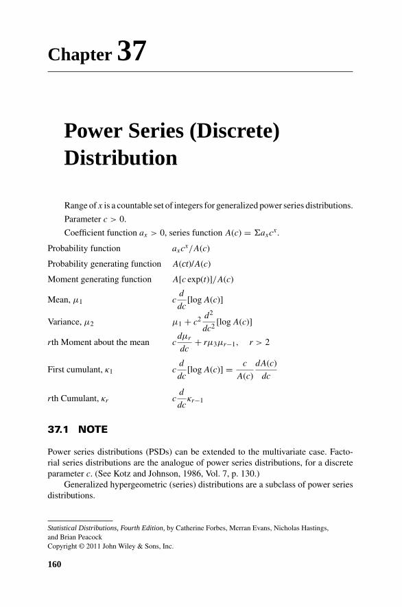
Chapter 37
Power Series (Discrete)Distribution
Range of x is a countable set of integers for generalized power series distributions.
Parameter c > 0.
Coefficient function ax > 0, series function A(c) = �axcx.
Probability function axcx/A(c)
Probability generating function A(ct)/A(c)
Moment generating function A[c exp(t)]/A(c)
Mean, μ1 cd
dc[log A(c)]
Variance, μ2 μ1 + c2 d2
dc2 [log A(c)]
rth Moment about the mean cdμr
dc+ rμ3μr−1, r > 2
First cumulant, κ1 cd
dc[log A(c)] = c
A(c)
dA(c)
dc
rth Cumulant, κr cd
dcκr−1
37.1 NOTE
Power series distributions (PSDs) can be extended to the multivariate case. Facto-rial series distributions are the analogue of power series distributions, for a discreteparameter c. (See Kotz and Johnson, 1986, Vol. 7, p. 130.)
Generalized hypergeometric (series) distributions are a subclass of power seriesdistributions.
Statistical Distributions, Fourth Edition, by Catherine Forbes, Merran Evans, Nicholas Hastings,and Brian PeacockCopyright © 2011 John Wiley & Sons, Inc.
160

37.3 Parameter Estimation 161
37.2 VARIATE RELATIONSHIPS
1. The binomial variate B: n, p is a PSD variate with parameter c = p/(1 − p)and series function A(c) = (1 + c)n = (1 − p)−n.
2. The Poisson variate P : λ is a PSD variate with parameter c = λ and seriesfunction A(c) = exp(c) and is uniquely characterized by having equal meanand variance for any c.
3. The negative binomial variate NB: x, p is a PSD variate with parameterc = 1 − p and series function A(c) = (1 − c)−x = p−x.
4. The logarithmic series variate is a PSD variate with parameter c and seriesfunction A(c) = − log(1 − c).
37.3 PARAMETER ESTIMATION
The estimator c of the shape parameter, obtained by the methods of maximum like-lihood or matching moments, is the solution of the equation
x = cd
dc[log A(c)] = c
A(c)
d[A(c)]
dc.

Chapter 38
Queuing Formulas
A queuing or waiting line system is where customers arrive for service, possiblywait in line, are served, and depart. Examples are supermarket checkouts, airlinecheck-ins, bank tellers, and so on. Queuing theory provides a classification systemand mathematical analysis of basic queuing models and this assists in the concep-tual understanding, design, and operation of queuing systems. Simulation techniquesprovide a way to create more elaborate models. Here we summarize the formulas fora number of the standard mathematical queuing models. Figure 38.1 illustrates thebasic situation of customers arriving, possibly waiting in a queue, being served, anddeparting.
38.1 CHARACTERISTICS OF QUEUING SYSTEMSAND KENDALL-LEE NOTATION
We can describe various types of queuing system in terms of six characteristics. Inthe following sections we introduce these characteristics, the Kendall-Lee notation,which is used to describe them, and some terms and symbols.
Characteristics of Queuing Systems
Arrival Pattern
Inter-arrival times at a queuing system follow a statistical distribution, commonlytaken to be a (negative) exponential distribution. The parameter λ (lambda) is theaverage arrival rate per unit time. An exponential arrival pattern is denoted by theletter M, for Markov, in the Kendall-Lee notation. The term Poisson arrivals is alsoused to describe this pattern, as the number of arrivals in any given time interval hasa Poisson distribution.
Statistical Distributions, Fourth Edition, by Catherine Forbes, Merran Evans, Nicholas Hastings,and Brian PeacockCopyright © 2011 John Wiley & Sons, Inc.
162

38.1 Characteristics of Queuing Systems and Kendall-Lee Notation 163
Arrivals Server 1
Server 2
Figure 38.1. A queuing system.
Service Time
The servers, assumed to be identical, have service times that follow a statistical distri-bution. If the distribution is exponential, the average service rate per server is denotedby μ. The mean service time per server for any service time distribution is denoted byτ. In the Kendall-Lee notation, an exponential service pattern is denoted by the letterM, a general service-time distribution is denoted by G, and a deterministic servicetime is denoted by D.
Number of Servers
The number of servers is denoted by s.
Queue Discipline
The queue discipline is the rule for taking items from the queue. The most common isfirst come first served, denoted by FCFS. Many mathematical results do not dependon the queue discipline and apply for a general discipline, denoted by G.
Maximum Number in System
The maximum number of customers in the system is denoted by C. The default valueis infinity, that is, no limit on the number of customers in the system.
Population
The size of the population from which the customers are drawn is denoted by N. Thedefault value is infinity, that is, no limit on the population from which the customersare drawn.
Customer Behavior
The following features of customer behavior sometimes occur. Analysis of queuesinvolving these behaviors is carried out by simulation rather than by application ofmathematical formulas.

164 Chapter 38 Queuing Formulas
• Balking is deciding not to join a queue dependent on its length;
• Reneging is leaving a queue after you have joined;
• Jockeying is switching from queue to queue in multiple queue systems.
Kendall-Lee Notation
Kendall-Lee notation is a shorthand way of describing a queuing system based on thecharacteristics just described. The value of each characteristic is denoted by its lettersymbol or a suitable numeric value, for example:
M/M/2/FCFS/6/∞
indicates a queuing system with Poisson arrivals, exponential service, two servers,first come first served (FCFS) queue discipline, a limit of six customers in the queueand an unlimited source of customers in the population.
38.2 DEFINITIONS, NOTATION, AND TERMINOLOGY
Steady State
Queuing formulas apply to steady state average values of properties such as theaverage length of the queue, the average time a customer spends in the queuingsystem and so on. Systems reach a steady state only if the arrival rate is less than themaximum service rate, or if excess arrivals are rejected by the system due to limitson the length of the queue.
Traffic Intensity and Traffic Density
For the basic M/M/1 queue the traffic intensity is the ratio of the arrival rate to theservice rate, and this must be less than one for the system to reach a steady state. Forother systems, the ratio of an arrival rate to a service rate appears in many queuingformulas. We refer to this quantity as the traffic density. The traffic density can bemore than one and the system will reach equilibrium if there are sufficient servers orif the there are queue restrictions. Figure 38.2 demonstrates the average number in anM/M/1 system as a function of the traffic intensity.
Notation and Terminology
Table 38.1 displays the symbols associated with the many varied queuing systemsdescribed in this chapter.
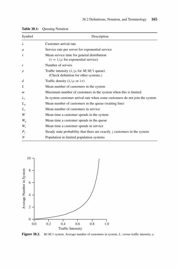
38.2 Definitions, Notation, and Terminology 165
Table 38.1: Queuing Notation
Symbol Description
λ Customer arrival rate
μ Service rate per server for exponential service
τ Mean service time for general distribution(τ = 1/μ for exponential service)
s Number of servers
ρ Traffic intensity (λ/μ for M/M/1 queue)(Check definition for other systems.)
d Traffic density (λ/μ or λτ)
L Mean number of customers in the system
m Maximum number of customers in the system when this is limited
λa In-system customer arrival rate when some customers do not join the system
Lq Mean number of customers in the queue (waiting line)
Ls Mean number of customers in service
W Mean time a customer spends in the system
Wq Mean time a customer spends in the queue
Ws Mean time a customer spends in service
Pj Steady state probability that there are exactly j customers in the system
N Population in limited population systems
Traffic Intensity
Ave
rage
Num
ber
in S
yste
m
0.0 0.2 0.4 0.6 0.8 1.0
10
8
6
4
2
0
Figure 38.2. M/M/1 system. Average number of customers in system, L, versus traffic intensity ρ.

166 Chapter 38 Queuing Formulas
38.3 GENERAL FORMULAS
Little’s formula,
L = λW
is based on equilibrium considerations and applies to a wide range of queuing systems.The formula simply asserts that the average number of customers in the system is equalto the customer arrival rate multiplied by the average time a customer spends in thesystem. Other general formulas are
Lq = λWq
Ws = τ
Ls = λWs = λτ
W = Wq + Ws = Wq + τ
L = Lq + Ls = Lq + λτ.
The delay ratio, denoted by H , is equal to the average time in the queue divided byaverage time in service, with
H = Wq/Ws = (L/λτ) − 1.
For equilibrium the maximum service rate must exceed the arrival rate
s > λτ
or, if some customers do not join, so that the in-system arrival rate is λa ≤ λ, then
s > λaτ.
38.4 SOME STANDARD QUEUING SYSTEMS
The M/M/1/G/∞/∞ System
This model has Poisson arrivals at rate λ, exponential service at rate μ, one server,and no limit on the queue length or the population. The formulas for this system areshown in Table 38.2.
Application
The practical result from this model is that for the queue to be kept at moderate lengththe traffic intensity should not exceed 0.75, that is, the arrival rate must not be morethan 75% of the service rate, and the server should be idle (or relaxed) 25% of the time.
The M/M/s/G/ ∞/∞ System
This model has Poisson arrivals at rate λ, exponential service at rate μ, s servers andno limit on the queue length or the population. The formulas for this system are shownin Table 38.3.

38.4 Some Standard Queuing Systems 167
Table 38.2: M/M/1/G/∞/∞ System Formulas
Description Symbol Formula
Traffic intensity ρ λ/μ
Probability server is idle P0 1 − ρ
Probability j customers in system Pj ρj (1 − ρ)
Probability server is busy ρ
Average number in system L ρ/ (1 − ρ) = λ/ (μ − λ)
Average number in queue Lq λ2/[μ (μ − λ)] = ρ2/ (1 − ρ)
Average number in service Ls ρ
Average time in system W 1/ (μ − λ)
Average time in queue Wq ρ/[μ (1 − ρ)]
Average time in service Ws 1/μ
Delay ratio H Wq/Ws = ρ/ (1 − ρ)
Table 38.3: M/M/s/G/∞/∞ System Formulas
Description Symbol Formula
Traffic intensity ρ λ/sμ
Traffic density d λ/μ
Probability all servers idle P0 1/[∑s−1
i=0 (sρ)i/i! + (sρ)s/s!(1 − ρ)]
Probability j customers in Pj P0(sρ)j/j!system for j = 1, 2, . . . , s
P0(sρ)j/[s!sj−s
]for j > s
Probability all servers busy Pj≥s P0(sρ)s/ [s!(1 − ρ)]
Proportion of servers busy ρ
Average number in queue Lq Pj≥s/(1 − ρ)
Average number in service Ls λ/μ = d
Average number in system L Lq + λ/μ
Average time in system W L/λ
Average time in queue Wq Pj≥s/(sμ − λ)
Average time in service Ws 1/μ
Delay ratio H Wq/Ws = μPj≥s/(sμ − λ)
For FCFS service discipline
Probability time in queue > t Pj≥s exp [−sμ (1 − ρ) t]

168 Chapter 38 Queuing Formulas
Table 38.4: M/G/1/G/∞/∞ System Formulas
Description Symbol Formula
Coefficient of variation of service time v σ/τ
distribution
Traffic intensity ρ λτ
Average number in queue Lq
(λ2σ2 + ρ2
)/[2 (1 − ρ)]
If the service time is deterministic, it’sstandard deviation is zero
Average number in queue, deterministic Lq(D) ρ2/[2(1 − ρ)]server
Ratio average number in queue for server Lq/Lq(D) v2 + 1with coefficient of variation, v
to deterministic server
Probability server is idle P0 1 − ρ
Probability server is busy ρ
Average number in system L Lq + ρ
Average number in service Ls ρ
Average time in queue Wq Lq/λ
Average time in system W Wq + 1/μ
Average time in service Ws τ
Delay ratio H Wq/Ws = Lq/(λτ)
Delay ratio relative to deterministic server H v2 + 1
The M/G/1/G/∞/∞ System (Pollaczek-Khinchin)
This model has Poisson arrivals at rate λ, a general service distribution with mean τ andstandard deviation σ, one server, and no limit on the queue length or the population.The results for this queue were derived by Pollaczek and Khinchin. The formulas forthis system are shown in Table 38.4.
Application
The practical result is that the queue length increases with the square of the coefficientof variation of the service time distribution. Hence the length of the queue in frontof a service facility will be reduced if the variability of the service time is reduced.Figure 38.3 displays the average length of the queue under this system as a functionof the coefficient of variation of service time.
The M/M/1/G/m/∞ System
This model has Poisson arrivals at rate λ, exponential service rate μ, one server, alimit of m on the number of customers in the system and no limit on the population.

38.4 Some Standard Queuing Systems 169
Coefficient of variation of service time, v
Ave
rage
leng
th o
f qu
eue
/ L
q(D)
0.0
0.5
1.0
1.5
2.0
2.5
3.0
3.5
0.0 0.5 1.0 1.5
Figure 38.3. M/G/1/G/∞/∞ system. Queue length as a function of the coefficient of variation ofthe service time distribution, as a multiple of the length for a deterministic server.
Arrivals who find that there are m customers in the system (or equivalently, m − 1 inthe queue) do not enter the system. Equilibrium can be achieved even with λ greaterthan or equal to μ, because arrivals who find the queue too long do not join the system.The formulas for this system are shown in Table 38.5.
The M/G/m/G/m/∞ System (Erlang)
This model has Poisson arrivals at rate λ, general service distribution with mean τ,m servers, a limit of m on the number in the system and no limit on the population.Arrivals who find that there are m customers in the system, that is, all servers arebusy, do not enter the system. Equilibrium can be achieved even with λ greater thanor equal to μ, because arrivals who find the queue too long do not join the system.The formulas for this system are shown in Table 38.6.
Application
This system was analyzed by Erlang for application to a telephone system wherem service channels were provided and customers who found them all busy wereassumed to be lost to the system. The probability that all servers are busy is Erlang’sloss formula. The analysis is used to choose a value of m, the number of servers, sothat the loss of customers is at an acceptable level.
The M/M/1/G/N/N System (One Server, FinitePopulation N)
This model has a finite population, N. A common application is where the itemsare machines and so we will refer to the items in the population as machines. Each
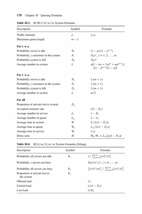
170 Chapter 38 Queuing Formulas
Table 38.5: M/M/1/G/m/∞ System Formulas
Description Symbol Formula
Traffic intensity ρ λ/μ
Maximum queue length m − 1
For λ /= μ
Probability server is idle P0 (1 − ρ)/(1 − ρm+1)
Probability j customers in the system Pj P0ρj, j = 1, 2, . . . , m
Probability system is full Pm P0ρm
Average number in system L p[1 − (m + 1)pm + mpm+1]/[(1 − pm+1)(1 − p)]
For λ = μ
Probability server is idle P0 1/(m + 1)
Probability j customers in the system Pj 1/(m + 1)
Probability system is full Pm 1/(m + 1)
Average number in system L m/2
For all
Proportion of arrivals lost to system Pm
Accepted customer rate λ(1 − Pm)
Average number in service Ls 1 − P0
Average number in queue Lq L − Ls
Average time in system W L/ [λ(1 − Pm)]
Average time in queue Wq Lq/ [λ(1 − Pm)]
Average time in service Ws 1/μ
Delay ratio H Wq/Ws = Lq/[ρ(1 − Pm)]
Table 38.6: M/G/m/G/m/∞ System Formulas (Erlang)
Description Symbol Formula
Probability all servers are idle P0 1/ [∑m
k=0(λτ)k/k!]
Probability j servers are busy P0(λτ)j/j!, j = 0, . . . , m
Probability all servers are busy Pm
[(λτ)m/m!
] / [∑m
k=0(λτ)k/k!]
Proportion of arrivals lost to Pm
the system
Offered load λτ
Carried load λτ(1 − Pm)
Lost load λτPm
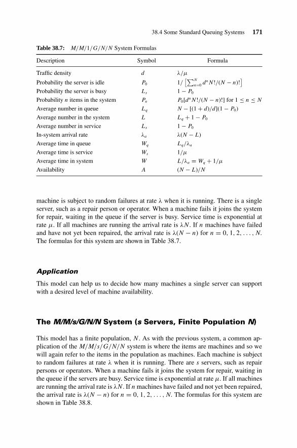
38.4 Some Standard Queuing Systems 171
Table 38.7: M/M/1/G/N/N System Formulas
Description Symbol Formula
Traffic density d λ/μ
Probability the server is idle P0 1/[∑N
n=0 dnN!/(N − n)!]
Probability the server is busy Ls 1 − P0
Probability n items in the system Pn P0[dnN!/(N − n)!] for 1 ≤ n ≤ N
Average number in queue Lq N − [(1 + d)/d](1 − P0)
Average number in the system L Lq + 1 − P0
Average number in service Ls 1 − P0
In-system arrival rate λa λ(N − L)
Average time in queue Wq Lq/λa
Average time is service Ws 1/μ
Average time in system W L/λa = Wq + 1/μ
Availability A (N − L)/N
machine is subject to random failures at rate λ when it is running. There is a singleserver, such as a repair person or operator. When a machine fails it joins the systemfor repair, waiting in the queue if the server is busy. Service time is exponential atrate μ. If all machines are running the arrival rate is λN. If n machines have failedand have not yet been repaired, the arrival rate is λ(N − n) for n = 0, 1, 2, . . . , N.
The formulas for this system are shown in Table 38.7.
Application
This model can help us to decide how many machines a single server can supportwith a desired level of machine availability.
The M/M/s/G/N/N System (s Servers, Finite Population N)
This model has a finite population, N. As with the previous system, a common ap-plication of the M/M/s/G/N/N system is where the items are machines and so wewill again refer to the items in the population as machines. Each machine is subjectto random failures at rate λ when it is running. There are s servers, such as repairpersons or operators. When a machine fails it joins the system for repair, waiting inthe queue if the servers are busy. Service time is exponential at rate μ. If all machinesare running the arrival rate is λN. If n machines have failed and not yet been repaired,the arrival rate is λ(N − n) for n = 0, 1, 2, . . . , N. The formulas for this system areshown in Table 38.8.

172 Chapter 38 Queuing Formulas
Table 38.8: M/M/s/G/N/N System Formulas
Description Symbol Formula
Traffic density d λ/μ
Probability the server is idle P0 1/∑s−1
n=0 dn[N!/(N − n)!n!]
+∑N
n=sdn[N!/(N − n)!s!sn−s]
Probability n items in the Pn P0(dn[N!/(N − n)!n!])system for 1 ≤ n ≤ s
P0(dn[N!/(N − n)!s!sn−s])for s < n ≤ N
Average number in queue Lq
∑N
n=s(n − s)Pn
Average number in the system L Lq + ∑s−1n=0 nPn + s
(1 − ∑s−1
n=0 Pn
)In-system arrival rate λa λ(N − L)
Average time in queue Wq Lq/λa
Average time is service Ws 1/μ
Average time in system W L/λa = Wq + 1/μ
Availability A (N − L)/N
Application
This model can help us to decide how many servers are needed to support a givennumber of machines at a desired level of machine availability.
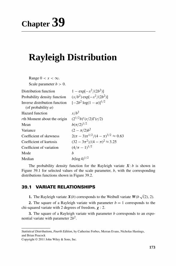
Chapter 39
Rayleigh Distribution
Range 0 < x < ∞.
Scale parameter b > 0.
Distribution function 1 − exp[−x2/(2b2)]
Probability density function (x/b2) exp[−x2/(2b2)]
Inverse distribution function [−2b2 log(1 − α)]1/2
(of probability α)
Hazard function x/b2
rth Moment about the origin (21/2b)r(r/2)�(r/2)
Mean b(π/2)1/2
Variance (2 − π/2)b2
Coefficient of skewness 2(π − 3)π1/2/(4 − π)3/2 ≈ 0.63
Coefficient of kurtosis (32 − 3π2)/(4 − π)2 ≈ 3.25
Coefficient of variation (4/π − 1)1/2
Mode b
Median b(log 4)1/2
The probability density function for the Rayleigh variate X: b is shown inFigure 39.1 for selected values of the scale parameter, b, with the correspondingdistributions functions shown in Figure 39.2.
39.1 VARIATE RELATIONSHIPS
1. The Rayleigh variate X(b) corresponds to the Weibull variate W(b√
(2), 2).
2. The square of a Rayleigh variate with parameter b = 1 corresponds to thechi-squared variate with 2 degrees of freedom, χ : 2.
3. The square of a Rayleigh variate with parameter b corresponds to an expo-nential variate with parameter 2b2.
Statistical Distributions, Fourth Edition, by Catherine Forbes, Merran Evans, Nicholas Hastings,and Brian PeacockCopyright © 2011 John Wiley & Sons, Inc.
173
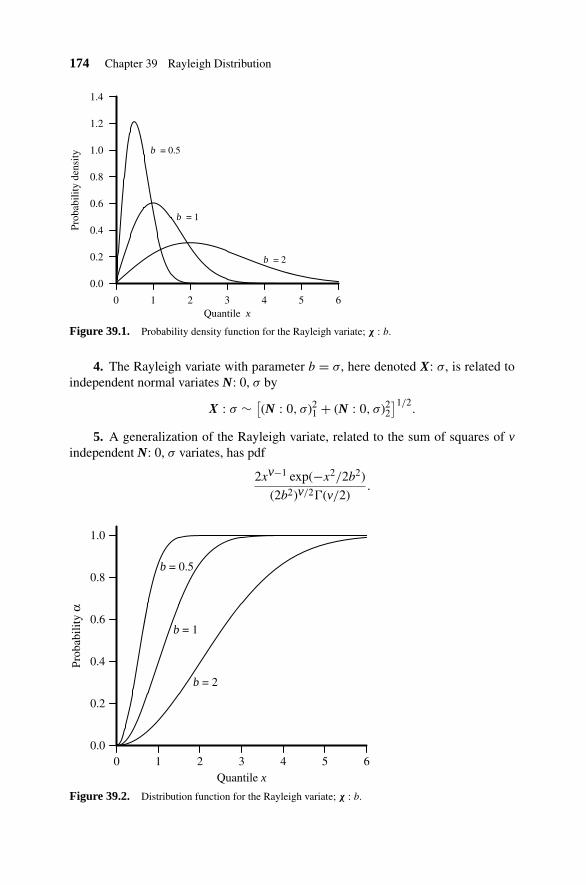
174 Chapter 39 Rayleigh Distribution
Quantile x
Prob
abili
ty d
ensi
ty
6543210
0.0
0.2
0.4
0.6
0.8
1.0
1.2
1.4
b = 0.5
b = 1
b = 2
Figure 39.1. Probability density function for the Rayleigh variate; χ : b.
4. The Rayleigh variate with parameter b = σ, here denoted X: σ, is related toindependent normal variates N: 0, σ by
X : σ ∼ [(N : 0, σ)2
1 + (N : 0, σ)22
]1/2.
5. A generalization of the Rayleigh variate, related to the sum of squares of vindependent N: 0, σ variates, has pdf
2xv−1 exp(−x2/2b2)
(2b2)v/2�(v/2).
Quantile x
Prob
abili
ty α
65432100.0
0.2
0.4
0.6
0.8
1.0
b = 0.5
b = 1
b = 2
Figure 39.2. Distribution function for the Rayleigh variate; χ : b.

39.2 Parameter Estimation 175
with rth moment about the origin
(21/2b)r�((r + v)/2
)�(v/2)
.
For b = 1, this corresponds to the chi variate χ : v.
39.2 PARAMETER ESTIMATION
Parameter Estimator Method/Properties
b(
12n
∑n
i=1 x2i
)1/2Maximum likelihood
Chapter 40
Rectangular (Uniform)Continuous Distribution
Every value in the range of the distribution is equally likely to occur. This is thedistribution taken by uniform random numbers. It is widely used as the basis for thegeneration of random numbers for other statistical distributions.
Variate R: a, b.
Where we write R without specifying parameters, we imply the standard or unitrectangular variate R: 0, 1.
Range a ≤ x ≤ b.
Location parameter a, the lower limit of the range. Parameter b, the upper limitof the range.
Distribution function (x − a)/(b − a)
Probability density function 1/(b − a)
Inverse distribution function (of probability α) a + α(b − a)
Inverse survival function (of probability α) b − α(b − a)
Hazard function 1/(b − x)
Cumulative hazard function − log[(b − x)/(b − a)]
Moment generating function [exp(bt) − exp(at)]/[t(b − a)]
Characteristic function [exp(ibt) − exp(iat)]/[it(b − a)]
rth Moment about the originbr+1 − ar+1
(b − a)(r + 1)
Mean (a + b)/2
Statistical Distributions, Fourth Edition, by Catherine Forbes, Merran Evans, Nicholas Hastings,and Brian PeacockCopyright © 2011 John Wiley & Sons, Inc.
176
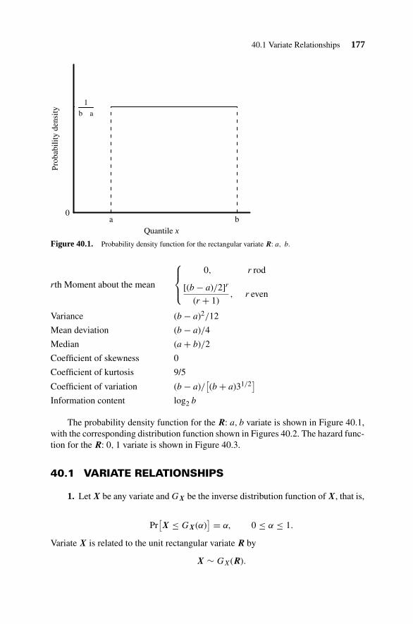
40.1 Variate Relationships 177
Quantile x
Prob
abili
ty d
ensi
ty
ba0
1
b − a
Figure 40.1. Probability density function for the rectangular variate R: a, b.
rth Moment about the mean
⎧⎪⎨⎪⎩
0, r rod
[(b − a)/2]r
(r + 1), r even
Variance (b − a)2/12
Mean deviation (b − a)/4
Median (a + b)/2
Coefficient of skewness 0
Coefficient of kurtosis 9/5
Coefficient of variation (b − a)/[(b + a)31/2
]Information content log2 b
The probability density function for the R: a, b variate is shown in Figure 40.1,with the corresponding distribution function shown in Figures 40.2. The hazard func-tion for the R: 0, 1 variate is shown in Figure 40.3.
40.1 VARIATE RELATIONSHIPS
1. Let X be any variate and GX be the inverse distribution function of X, that is,
Pr[X ≤ GX(α)
] = α, 0 ≤ α ≤ 1.
Variate X is related to the unit rectangular variate R by
X ∼ GX(R).

178 Chapter 40 Rectangular (Uniform) Continuous Distribution
Quantile x
Prob
abili
ty α
ba0
1
Figure 40.2. Distribution function for the rectangular variate R: a, b.
Quantile x
Haz
ard
0.0 0.5 1.0
1
5
10
Figure 40.3. Hazard function for the unit rectangular variate R: 0, 1.
For X any variate with a continuous density function fX(x), the cdf of x, fX(x),satisfies
FX(x) ∼ R : 0, 1.
2. The distribution function of the sum of n-independent unit rectangular variatesRi, i = 1, . . . , n is
k∑i=0
(−1)i(
n
i
)(x − i)n
n!, k ≤ x ≤ k + 1, k = 0, 1, . . . , n − 1.

40.3 Random Number Generation 179
3. The unit parameter beta variate β: 1, 1 and the power function variate, heredenoted X: 1, 1, correspond to a unit rectangular variate R.
4. The mean of two independent unit rectangular variates is a standard symmet-rical triangular variate.
40.2 PARAMETER ESTIMATION
Parameter Estimator Method
Lower limit, a x − 31/2s Matching moments
Upper limit, b x + 31/2s Matching moments
40.3 RANDOM NUMBER GENERATION
Algorithms to generate pseudorandom numbers, which closely approximate indepen-dent standard unit rectangular variates, R: 0, 1, are a standard feature in statisticalsoftware.

Chapter 41
Rectangular (Uniform)Discrete Distribution
In sample surveys it is often assumed that the items (e.g., people) being surveyed areuniformly distributed through the sampling frame.
Variate D: 0, n.
Range 0 ≤ x ≤ n, x an integer taking values 0, 1, 2, . . ., n.
Distribution function (x + 1)/(n + 1)
Probability function 1/(n + 1)
Inverse distribution function (of probability α) α(n + 1) − 1
Survival function (n − x)/(n + 1)
Inverse survival function (of probability α) n − α(n + 1)
Hazard function 1/(n − x)
Probability generating function (1 − tn+1)/[(n + 1)(1 − t)]
Characteristic function {1 − exp[it(n + 1)]}/{[1 − exp(it)](n + 1)}
Moments about the origin
Mean n/2
Second n(2n + 1)/6
Third n2(n + 1)/4
Variance n(n + 2)/12
Coefficient of skewness 0
Coefficient of kurtosis3
5[3 − 4/n(n + 2)]
Coefficient of variation [(n + 2)/3n]1/2
The probability function for the D : 0, n variate is shown in Figure 41.1, withthe corresponding distribution function shown in Figure 41.2.
Statistical Distributions, Fourth Edition, by Catherine Forbes, Merran Evans, Nicholas Hastings,and Brian PeacockCopyright © 2011 John Wiley & Sons, Inc.
180

41.2 General Form 181
Quantile x
Prob
abili
ty
1
n + 1
0 n
Figure 41.1. Probability function for the discrete rectangular variate D: 0, n.
41.1 GENERAL FORM
Let a ≤ x ≤ a + nh, such that any point of the sample space is equally likely. The terma is a location parameter and h, the size of the increments, is a scale parameter. Theprobability function is still 1/(n + 1). The mean is a + nh/2, and the rth momentsare those of the standard form D: 0, 1 multiplied by hr.
As N tends to infinity and h tends to zero with nh = b − a, the discrete rectan-gular variate D: a, a + nh tends to the continuous rectangular variate R: a, b.
Quantile x
Prob
abili
ty α
0
1
0 n
Figure 41.2. Distribution function for the discrete rectangular variate D: 0, n.

182 Chapter 41 Rectangular (Uniform) Discrete Distribution
41.2 PARAMETER ESTIMATION
Parameter Estimator Method/Properties
Location parameter, a x − nh/2 Matching moments
Increments, h{
12s2/[n(n − 2)]}1/2
Matching moments

Chapter 42
Student’s t Distribution
The Student’s t distribution is used to test whether the difference between the meansof two samples of observations is statistically significant. For example, the heightsof a random sample of basketball players could be compared with the heights from arandom sample of football players. The Student’s t distribution would be used to testwhether the data indicated that one group was significantly taller than the other. Moreprecisely, it would be testing the hypothesis that both samples were drawn from thesame normal population. A significant value of t would cause the hypothesis to berejected, indicating that the means were significantly different.
Variate t: ν.
Range −∞ < x < ∞.
Shape parameter ν, degrees of freedom, ν a positive integer.
Distribution function
⎧⎪⎪⎪⎪⎪⎪⎪⎪⎪⎪⎪⎪⎪⎪⎪⎪⎪⎪⎪⎨⎪⎪⎪⎪⎪⎪⎪⎪⎪⎪⎪⎪⎪⎪⎪⎪⎪⎪⎪⎩
1
2+ 1
πtan−1
( x
ν1/2
)
+ 1
π
xν1/2
ν + x2
⎡⎣(ν−3)/2∑
j=0
aj
(1 + x2/ν)j
⎤⎦ , ν odd
1
2+ x
2(ν + x2)1/2
(ν−2)/2∑j=0
bj(1 + x2
ν
)j, ν even
where aj = [2j/(2j + 1)]aj−1, a0 = 1
bj = [(2j − 1)/2j]bj−1, b0 = 1
Probability density function{�[(ν + 1)/2]}
(πν)1/2�(ν/2)[1 + (x2/ν)](ν+1)/2
Mean 0, ν > 1
Statistical Distributions, Fourth Edition, by Catherine Forbes, Merran Evans, Nicholas Hastings,and Brian PeacockCopyright © 2011 John Wiley & Sons, Inc.
183

184 Chapter 42 Student’s t Distribution
Quantile x
Prob
abili
ty d
ensi
ty
−3 −2 −1 3210
0.0
0.25
0.5
ν = 1
ν = 5
ν = 100
Figure 42.1. Probability density function for Student’s t variate, t: ν.
rth Moment about the mean
⎧⎨⎩
μr = 0, r odd
μr = 1 · 3 · 5 · · · (r − 1)νr/2
(ν − 2)(ν − 4) · · · (ν − r)r even, ν > r
Variance ν/(ν − 2), ν > 2
Mean deviation ν1/2�
[1
2(ν − 1)
] / [π1/2�
(1
2ν
)]
Mode 0
Coefficient of skewness 0, ν > 3 (always symmetrical)
Coefficient of kurtosis 3(ν − 2)/(ν − 4), ν > 4
Quantile x
−3 −2 −1 3210
0.5
1.0
ν = 1
ν = 5 ν = 100Probability α
Figure 42.2. Distribution function for Student’s t variate, t : ν.

42.1 Variate Relationships 185
The probability density function for the Student’s t variate t : v is shown inFigure 42.1 for selected values of the degrees of freedom parameter, v, with thecorresponding distributions functions shown in Figure 42.2.
42.1 VARIATE RELATIONSHIPS
1. The Student’s t variate with ν degrees of freedom, t: ν, is related to the inde-pendent chi-squared variate χ2 : ν, the F variate F: 1, ν, and the unit normal variateN: 0, 1 by
(t : ν)2 ∼ (χ2 : 1
)/[(
χ2 : ν)/ν
]∼ F : 1, ν
∼ (N : 0, 1)2/[(
χ2 : ν)/ν
]
t : ν ∼ (N : 0, 1)/[(
χ2 : ν)/ν
]1/2.
Equivalently, in terms of a probability statement,
Pr[(t : ν) ≤ x] = 1
2
{1 + Pr
[(F : 1, ν) ≤ x2]}.
In terms of the inverse survival function of t : ν at probability level 12α, denoted
Zt( 1
2α : ν), and the survival function of the F variate F : 1, ν at probability level α,
denoted ZF (α : 1, ν), the last equation is equivalent to
[Zt
(1
2α : ν
)]2
= ZF (α : 1, ν).
2. As ν tends to infinity, the variate t : ν tends to the unit normal variate N: 0,1.The approximation is reasonable for ν ≥ 30.
t : ν ≈ N : 0, 1; ν ≥ 30.
3. Consider independent normal variates N : μ, σ. Define variates x, s2 asfollows:
x ∼(
1
n
) n∑i=1
(N : μ, σ)i, s2 ∼(
1
n
) n∑i=1
[(N : μ, σ)i − x]2.
Then
t : n − 1 ∼ x − μ
s/(n − 1)1/2 .
4. Consider a set of n1-independent normal variates N : μ1, σ, and a setof n2-independent normal variates N : μ2, σ. Define variates x1, x2, s
21, s
22 as

186 Chapter 42 Student’s t Distribution
follows:
x1 ∼(
1
n1
) n1∑i=1
(N : μ1, σ)i,
x2 ∼(
1
n2
) n2∑j=1
(N : μ2, σ)j
s21 ∼
(1
n1
) n1∑i=1
[(N : μ1, σ)i − x1
]2
s22 ∼
(1
n2
) n2∑j=1
[(N : μ2, σ)j − x2
]2.
Then
t : n1 + n2 − 2 ∼ (x1 − x2) − (μ1 − μ2)(n1s
21 + n2s
22
n1 + n2 − 2
)1/2 (1
n1+ 1
n2
)1/2.
5. The t: 1 variate corresponds to the standard Cauchy variate, C : 0, 1.
6. The t : ν variate is related to two independent F : ν, ν variates by
(ν1/2/2)[(F : ν, ν)1/2
1 − (F : ν, ν)−1/22
]∼ t : ν.
7. Two independent chi-squared variates χ2 : ν are related to the t : ν variate by(ν1/2
2
) [(χ2 : ν)1 − (χ2 : ν)2
][(χ2 : ν)1(χ2 : ν)2
]1/2 ∼ t : ν.
42.2 RANDOM NUMBER GENERATION
From independent N: 0, 1 and χ2 : ν variates
t : ν ∼ N : 0, 1√(χ2 : ν)/ν
or from a set of ν + 1 independent N: 0, 1 variates
t : ν ∼ (N : 0, 1)ν+1√ν∑
i=1(N : 0, 1)2
i /ν
.

Chapter 43
Student’s t (Noncentral)Distribution
The noncentral t distribution can be applied to the testing of one-sided hypothesesrelated to normally distributed data. For example, if the mean test score of a largecohort of students is known, then it would be possible to test the hypothesis that themean score of a subset, from a particular teacher, was higher than the general meanby a specified amount.
Variate t: ν, δ.
Range −∞ < x < ∞.
Shape parameters ν a positive integer, the degrees of freedom and −∞ < δ < ∞,the noncentrality parameter.
Probability density function(ν)ν/2 exp(−δ2/2)
�(ν/2)π1/2(ν + x2)(ν+1)/2
×∞∑i=0
�
(ν + i + 1
2
)(xδ)i
i!
(2
ν + x2
)i/2
rth Moment about the origin (ν/2)r/2�((ν − r)/2)/�(ν/2)
×r/2∑j=0
(r
2j
)(2j)!δr−2j/(2jj!), ν > r
Meanδ(ν/2)1/2�((ν − 1)/2)
�(ν/2), ν > 1
Varianceν
(ν − 2)(1 + δ2) − ν
2δ2
(�((ν − 1)/2)
�(ν/2)
)2
, ν > 2
Statistical Distributions, Fourth Edition, by Catherine Forbes, Merran Evans, Nicholas Hastings,and Brian PeacockCopyright © 2011 John Wiley & Sons, Inc.
187
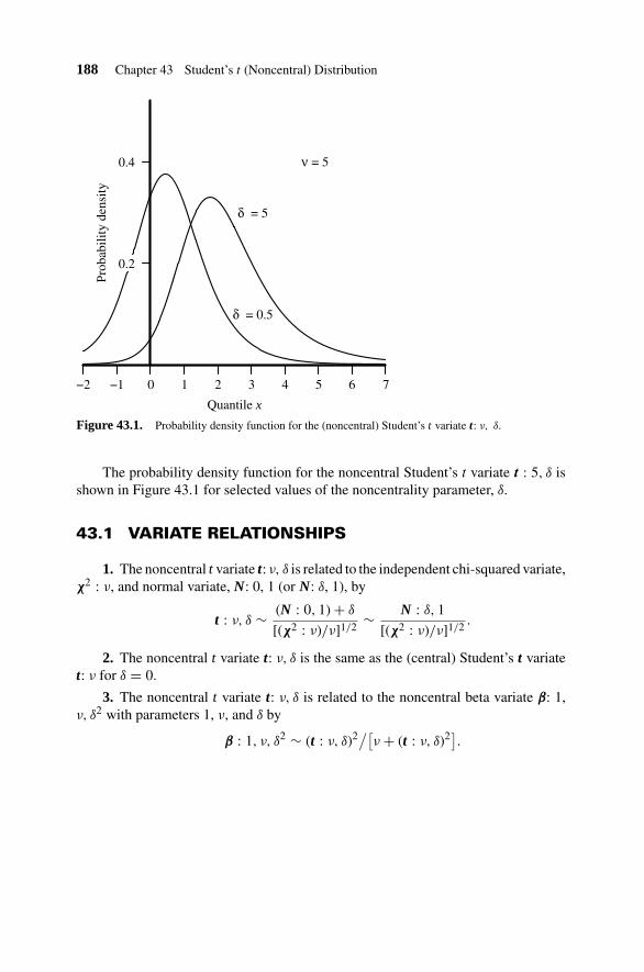
188 Chapter 43 Student’s t (Noncentral) Distribution
Quantile x
Prob
abili
ty d
ensi
ty
−2 −1 76543210
0.2
0.4 ν = 5
δ = 5
δ = 0.5
Figure 43.1. Probability density function for the (noncentral) Student’s t variate t: ν, δ.
The probability density function for the noncentral Student’s t variate t : 5, δ isshown in Figure 43.1 for selected values of the noncentrality parameter, δ.
43.1 VARIATE RELATIONSHIPS
1. The noncentral t variate t: ν, δ is related to the independent chi-squared variate,χ2 : ν, and normal variate, N: 0, 1 (or N: δ, 1), by
t : ν, δ ∼ (N : 0, 1) + δ
[(χ2 : ν)/ν]1/2 ∼ N : δ, 1
[(χ2 : ν)/ν]1/2 .
2. The noncentral t variate t: ν, δ is the same as the (central) Student’s t variatet: ν for δ = 0.
3. The noncentral t variate t: ν, δ is related to the noncentral beta variate β: 1,ν, δ2 with parameters 1, ν, and δ by
β : 1, ν, δ2 ∼ (t : ν, δ)2/[ν + (t : ν, δ)2].

Chapter 44
Triangular Distribution
Range a ≤ x ≤ b.
Parameters: Shape parameter c, the mode.
Location parameter a, the lower limit; parameter b, the upper limit.
Distribution function
⎧⎪⎪⎪⎨⎪⎪⎪⎩
(x − a)2
(b − a)(c − a), if a ≤ x ≤ c
1 − (b − x)2
(b − a)(b − c), if c ≤ x ≤ b
Probability density function
⎧⎨⎩
2(x − a)/[(b − a)(c − a)], if a ≤ x ≤ c
2(b − x)/[(b − a)(b − c)], if c ≤ x ≤ b
Mean (a + b + c)/3
Variance (a2 + b2 + c2 − ab − ac − bc)/18
Mode c
The probability density function for the triangular variate for selected values ofthe shape parameter, c, relative to the two location parameters, a and b, are shown inFigure 44.1.
44.1 VARIATE RELATIONSHIPS
1. The standard triangular variate corresponding to a = 0, b = 1, has median√c/2 for c ≥ 1
2 and 1 − √(1 − c)/2 for c ≤ 1
2 .
2. The standard symmetrical triangular variate is a special case of the tri-angular variate with a = 0, b = 1, c = 1
2 . It has even moments about the mean
Statistical Distributions, Fourth Edition, by Catherine Forbes, Merran Evans, Nicholas Hastings,and Brian PeacockCopyright © 2011 John Wiley & Sons, Inc.
189
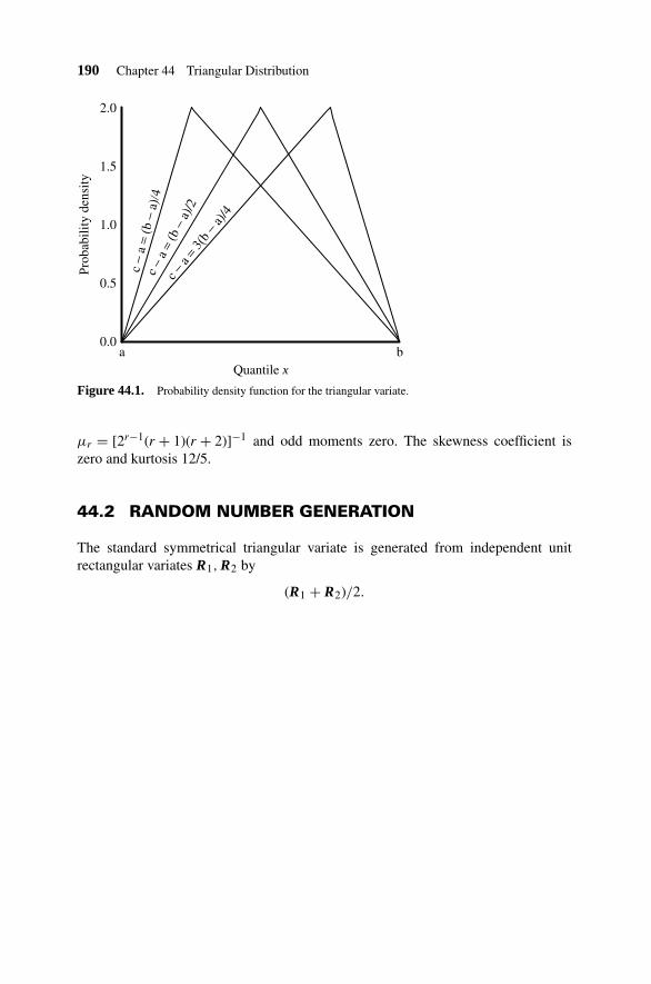
190 Chapter 44 Triangular Distribution
Quantile x
Prob
abili
ty d
ensi
ty
ba0.0
0.5
1.0
1.5
2.0
c −
a =
(b −
a)/4
c −
a =
(b −
a)/2
c − a
= 3(b
− a)/4
Figure 44.1. Probability density function for the triangular variate.
μr = [2r−1(r + 1)(r + 2)]−1 and odd moments zero. The skewness coefficient iszero and kurtosis 12/5.
44.2 RANDOM NUMBER GENERATION
The standard symmetrical triangular variate is generated from independent unitrectangular variates R1, R2 by
(R1 + R2)/2.
Chapter 45
von Mises Distribution
Range 0 < x ≤ 2π, where x is a circular random variate.
Scale parameter b > 0 is the concentration parameter.
Location parameter 0 ≤ a < 2π is the mean direction.
Distribution function [2πI0(b)]−1
{xI0(b) + 2
∞∑j=0
Ij(b)sin j(x − a)
j
},
where It(b) =(
b
2
)t ∞∑i=0
(b2/4)t
i!�(t + i + 1)
is the modified Bessel functionof the first kind of order t;
for order t = 0, I0(b) =∞∑i=0
b2i/[22i(i!)2]
Probability density function exp[b cos(x − a)]/(2πI0(b))
Characteristic function [It(b)/I0][cos(at) + i sin(at)]
rth Trigonometric momentabout the origin
{[Ir(b)/I0(b)] cos(ar)
[Ir(b)/I0(b)] sin(ar)Mean direction a
Mode a
Circular variance 1 − I1(b)/I0(b)
45.1 NOTE
The von Mises distribution can be regarded as the circular analogue of the normaldistribution on the line. The distribution is unimodal, symmetric about a, and infinitelydivisible. The minimum value occurs at a ± π [whichever is in range (0, 2π)], andthe ratio of maximum to minimum values of the pdf is exp(2b).
Statistical Distributions, Fourth Edition, by Catherine Forbes, Merran Evans, Nicholas Hastings,and Brian PeacockCopyright © 2011 John Wiley & Sons, Inc.
191

192 Chapter 45 von Mises Distribution
Quantile x
Prob
abili
ty d
ensi
ty
0 π 2 π 3π 2 2π
2
4
b = 1.5
b = 2
b = 1
a = π
Figure 45.1. Probability density function for the von Mises variate.
The probability density function for the von Mises variate with location parametera = π and for selected values of the scale parameter, b, are shown in Figure 45.1.
45.2 VARIATE RELATIONSHIPS
1. For b = 0, the von Mises variate reduces to the rectangular variate R: a, bwith a = 0, b = 2π with pdf 1/(2π).
2. For large b, the von Mises variate tends to the normal variate N: μ, σ withμ = 0, σ = 1/b.
3. For independent normal variates, with means sin(a) and cos(a), respectively,let their corresponding polar coordinates be R and θ. The conditional distribution ofθ, given R = 1, is the von Mises distribution with parameters a and b.
45.3 PARAMETER ESTIMATION
Parameter Estimator Method/Properties
a tan−1
(n∑
i=1
sin xi
/ n∑i=1
cos xi
)Maximum likelihood
I1(b)/I0(b)(a measure of precision)
1
n
[(n∑
i=1
cos xi
)2
+(
n∑i=1
sin xi
)2]1/2
Maximum likelihood

Chapter 46
Weibull Distribution
The Weibull variate is commonly used as a lifetime distribution in reliability applica-tions. The two-parameter Weibull distribution can represent decreasing, constant, orincreasing failure rates. These correspond to the three sections of the “bathtub curve”of reliability, referred to also as “burn-in,” “random,” and “wearout” phases of life.The bi-Weibull distribution can represent combinations of two such phases of life.
Variate W : η, β.
Range 0 ≤ x < ∞.
Scale parameter η > 0 is the characteristic life.
Shape parameter β > 0.
Distribution function 1 − exp[−(x/η)β]
Probability density function (βxβ−1/ηβ) exp[−(x/η)β]
Inverse distribution function η{log[1/(1 − α)]}1/β
(of probability α)
Survival function exp[−(x/η)β]
Inverse survival function η[log(1/α)1/β](of probability α)
Hazard function βxβ−1/ηβ
Cumulative hazard function (x/η)β
rth Moment about the origin ηr�[(β + r)/β]
Mean η�[(β + 1)/β]
Variance η2(�[(β + 2)/β] − {�[(β + 1)/β]}2)
Mode
{η(1 − 1/β)1/β, β≥1
0, β≤1
Statistical Distributions, Fourth Edition, by Catherine Forbes, Merran Evans, Nicholas Hastings,and Brian PeacockCopyright © 2011 John Wiley & Sons, Inc.
193

194 Chapter 46 Weibull Distribution
Quantile x
Prob
abili
ty d
ensi
ty
210 30.0
0.2
0.4
0.6
0.8
1.0
1.2
1.4
=β 0.5
=β 1
=β 3
=η 1
Figure 46.1. Probability density function for the Weibull variate. W : η, β.
Median η(log 2)1/β
Coefficient of variation
(�[(β + 2)/β]
{�[(β + 1)/β]}2 − 1
)1/2
The probability density function for the W: 1, β variate for selected values ofthe shape parameter, β, is shown in Figure 46.1, with the corresponding distributionfunctions shown in Figure 46.2 and the corresponding hazard functions shown inFigure 46.3. The relationship between the shape parameter, β, and the mean andstandard deviation of the W: 1, β variate is shown in Figure 46.4.
Quantile x
Prob
abili
ty d
ensi
ty
210 30.0
0.2
0.4
0.6
0.8
1.0
β = 0.5
β = 1β = 3
η = 1
Figure 46.2. Distribution function for the Weibull variate. W : η, β.
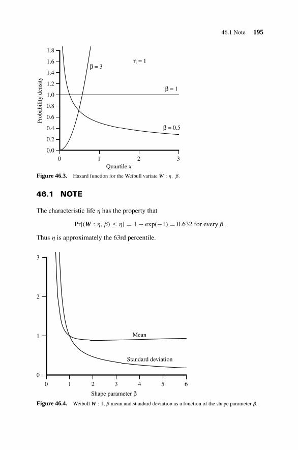
46.1 Note 195
Quantile x
Prob
abili
ty d
ensi
ty
210 30.0
0.2
0.4
0.6
0.8
1.0
1.2
1.4
1.6
1.8
β = 0.5
β = 1
β = 3η = 1
Figure 46.3. Hazard function for the Weibull variate W : η, β.
46.1 NOTE
The characteristic life η has the property that
Pr[(W : η, β) ≤ η] = 1 − exp(−1) = 0.632 for every β.
Thus η is approximately the 63rd percentile.
Shape parameter β6543210
0
1
2
3
Mean
Standard deviation
Figure 46.4. Weibull W : 1, β mean and standard deviation as a function of the shape parameter β.

196 Chapter 46 Weibull Distribution
46.2 VARIATE RELATIONSHIPS
1. The standard Weibull variate has a characteristic life value η = 1. The generalWeibull variate W: η, β is a sealed standard Weibull variate.
W : η, β ∼ η(W : 1, β),2. The Weibull variate W : η, β with shape parameter β = 1 is the exponential
variate E : η with mean η,
W : η, 1 ∼ E : η.
The Weibull variate W : η, β is related to E : η by (W : η, β)β ∼ E : ηβ.
3. The Weibull variate W : η, 2 is the Rayleigh variate, and the Weibull variateW : η, β is also known as the truncated Rayleigh variate.
4. The Weibull variate W : η, βη is related to the standard extreme value(Gumbel) variate V: 0, 1 by
−β log[(W : η, β)/η] ∼ V : 0, 1.
46.3 PARAMETER ESTIMATION
By the method of maximum likelihood the estimators, η, β, of the shape and scaleparameters are the solution of the simultaneous equations:
η =[(
1
n
) n∑i=1
xβi
]1/β
β = n
(1/η)n∑
i=1xβi log xi −
n∑i=1
log xi
.
46.4 RANDOM NUMBER GENERATION
Random numbers of the Weibull variate W : η, β can be generated from those of theunit rectangular variate R using the relationship
W : η, β ∼ η(− log R)1/β.
46.5 THREE-PARAMETER WEIBULL DISTRIBUTION
Further flexibility can be introduced into the Weibull distribution by adding a thirdparameter, which is a location parameter and is usually denoted by the symbol gamma(γ). The probability density is zero for x < γ and then follows a Weibull distributionwith origin at γ . In reliability applications, gamma is often referred to as the minimumlife, but this does not guarantee that no failures will occur below this value in the future.
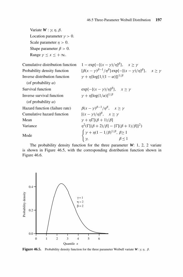
46.5 Three-Parameter Weibull Distribution 197
Variate W : γ, η, β.
Location parameter γ > 0.
Scale parameter η > 0.
Shape parameter β > 0.
Range γ ≤ x ≤ + ∞.
Cumulative distribution function 1 − exp{−[(x − γ)/η]β}, x ≥ γ
Probability density function [β(x − γ)β−1/ηβ] exp{−[(x − γ)/η]β}, x ≥ γ
Inverse distribution function γ + η{log[1/(1 − α)]}1/β
(of probability α)
Survival function exp{−[(x − γ)/η]β}, x ≥ γ
Inverse survival function γ + η[log(1/α)]1/β
(of probability α)
Hazard function (failure rate) β(x − γ)β−1/ηβ, x ≥ γ
Cumulative hazard function [(x − γ)/η]β, x ≥ γ
Mean γ + η�[(β + 1)/β]
Variance η2(�[(β + 2)/β] − {�[(β + 1)/β]}2)
Mode
{γ + η(1 − 1/β)1/β, β≥ 1
γ, β ≤ 1
The probability density function for the three parameter W: 1, 2, 2 variateis shown in Figure 46.5, with the corresponding distribution function shown inFigure 46.6.
Quantile x
Prob
abili
ty d
ensi
ty
6543210
0.0
0.2
0.4
γ = 1η = 2β = 2
Figure 46.5. Probability density function for the three parameter Weibull variate W: γ, η, β.

198 Chapter 46 Weibull Distribution
Quantile x
Prob
abili
ty α
6543210
0.0
0.5
1.0
γ = 1η = 2β = 2
Figure 46.6. Distribution function for the three parameter Weibull variate W: γ, η, β.
46.6 THREE-PARAMETER WEIBULL RANDOM NUMBERGENERATION
Random numbers of the Weibull variate W: γ, η, β can be generated from the unitrectangular variate R using the relationship
W : γ, η, β ∼ γ + η(− log R)1/β.
46.7 BI-WEIBULL DISTRIBUTION
A bi-Weibull distribution is formed by combining two Weibull distributions. Thisprovides a distribution model with a very flexible shape. In reliability analysis, forexample, it can represent combinations of (two of) decreasing, constant, and/or in-creasing failure rates. Even more flexibility can be introduced by adding more than twoWeibull distributions, but this increases the number of parameters to be estimated. Sev-eral versions of the bi-Weibull distribution have been proposed by different authors.These versions differ in the way in which the two Weibull distributions are combined,and in the number of parameters specified. The five-parameter bi-Weibull distributiondescribed here is used in the RELCODE software package (www.albanyint.com.au).
46.8 FIVE-PARAMETER BI-WEIBULL DISTRIBUTION
W : λ, θ, γ, η, β.
Phase 1 scale parameter λ > 0, shape parameter θ > 0.
Phase 2 location parameter γ ≥ 0, scale parameter η > 0, shape parameter β > 0.

46.8 Five-Parameter Bi-Weibull Distribution 199
A five-parameter bi-Weibull distribution is derived by adding two Weibull hazardfunctions. The first of these hazard functions is a two-parameter Weibull hazard func-tion with the equation
h(x) = λθ(λx)θ−1
where x is the component age, h(x) is the hazard function at age x, λ is the reciprocalof a scale parameter, and θ is a shape parameter. The case where θ = 1 correspondsto a constant failure rate λ. The second hazard function is a three-parameter Weibullhazard function, which becomes operative for x > γ . The equation is
h(x) =(
β
η
) ((x − γ)
η
)β−1
here, β, η, and γ are shape, scale, and location parameters, respectively, as in thethree-parameter Weibull distribution.
Adding the two hazard functions gives the five-parameter bi-Weibull distribution,for which the hazard and reliability equations are:
Hazard function
h(x) =
⎧⎪⎨⎪⎩
λθ(λx)θ−1 0 < x < γ
λθ(λx)θ−1 +(
β
η
) ((x − γ)
η
)β−1
x ≥ γ
Survival function
S(x) ={
e−(λx)θ 0 < x < γ
exp(−{(λx)θ + [(x − γ)/η]β}) x ≥ γ
Quantile x
Haz
ard
0 8642 10 12 14
0
1
2
3
4
5
λ = 0.1
θ = 0.7
γ =4
η = 4β = 3
Figure 46.7. Bi-Weibull hazard function W: λ, θ, γ, η, β.

200 Chapter 46 Weibull Distribution
Quantile x
Haz
ard
840 12
0.15
0.3 =λ 0.1
=θ 0.7=γ 4
=η 4
=β 3
Figure 46.8. Bi-Weibull probability density function W: λ, θ, γ, η, β.
Bi-Weibull Random Number Generation
Use the equations given for the bi-Weibull survival function S(x) to calculate valuesof S(x), for values of x from 0 to γ + 2η, and keep the results in a table. Generatea uniform random number R and look up the value of x corresponding to S(x) = R(approximately) in the table.
Bi-Weibull Graphs
Figures 46.7, 46.8, 46.9 show, respectively, examples of the five-parameter bi-Weibullhazard function, probability density function, and reliability function. Note that the
Quantile x
Prob
abili
ty α
840 12
0.5
1.0
λ = 0.1
θ = 0.7γ = 4
η = 4
β = 3
Figure 46.9. Bi-Weibull distribution function W: λ, θ, γ, η, β.

46.9 Weibull Family 201
hazard function has a “bathtub” shape, which in a reliability application correspondsto a combination of burn-in and wearout failures. The range of shapes that can betaken by the bi-Weibull distribution is large. Any combination of two Weibull failurerate patterns can be accommodated, for example, burn-in plus wearout, random pluswearout, burn-in plus random, random plus another random starting later. β is notrequired to be greater than 1, nor θ less than 1. In practice, the use of the five-parameterbi-Weibull distribution to detect the onset of wearout is one of its main advantages.
46.9 WEIBULL FAMILY
The negative exponential, two-parameter Weibull, three-parameter Weibull, andbi-Weibull distributions form a family of distributions of gradually increasingcomplexity.
The negative exponential is the simplest and has a constant hazard function. Thetwo-parameter Weibull extends the range of models to include (one of) decreasing,constant, or increasing hazard function. The three-parameter Weibull model adds alocation parameter to the two-parameter model. The bi-Weibull distribution allows(two of) decreasing, constant, and increasing hazard function.

Chapter 47
Wishart (Central) Distribution
Matrix variate: WC: k, n, �.
Formed from n-independent multinormal variates MN: μ, � by
WC: k, n,� ∼n∑
i=1
(MN: μi, � − μi)(MN: μi, � − μi)′.
Matrix quantile X a k × k positive semidefinite matrix, with elementsXij .
Parameters k, n ≥ k, �, where k is the dimension of the n-associated multinormalmultivariates; n is the degrees of freedom, n ≥ k; and � is the k × k variance-covariance matrix of the associated multinormal multivariates, with elements�ij = σij .
Distribution function�k[(k + 1)/2]|X|n/2
1F1
(n/2; (k + 1)/2; − 1
2�−1X)
�k
[12 (n + k + 1)
]|2�|n/2
where 1F1 is a hypergeometric functionof the matrix argument
Probability density function exp
(−1
2tr�−1X
)|X|(n−k−1)/2
/ {�k
(n
2
)|2�|n/2
}
Characteristic function |Ik − 2i�T |−n/2, where T is asymmetric k × k matrix such that�−1 − 2T is positive define
Moment generating function |Ik − 2�T |−n/2
rth Moment about origin |2�|r�k
(1
2n + r
) /�k
(1
2n
)
Mean n�
Individual elements E(Xij) = nσij
cov(Xij, Xrs) = n(σirσjs + σisσjr)
Statistical Distributions, Fourth Edition, by Catherine Forbes, Merran Evans, Nicholas Hastings,and Brian PeacockCopyright © 2011 John Wiley & Sons, Inc.
202
47.2 Variate Relationships 203
47.1 NOTE
The Wishart variate is a k-dimensional generalization of the chi-squared variate,which is the sum of squared normal variates. It performs a corresponding role formultivariate normal problems as the chi-squared does for the univariate normal.
47.2 VARIATE RELATIONSHIPS
1. The Wishart k × k matrix variate WC: k, n, � is related to n-independentmultinormal multivariates of dimension k, MN: μ,�, by
WC : k, n,� ∼n∑
i=1
(MN : μi, � − μi)(MN : μi, � − μi)′.
2. The sum of mutually independent Wishart variates WC: k, ni, � is also aWishart variate with parameters k, �ni, �.∑
(WC : k, ni, �) ∼ WC : k,∑
ni, �.
Chapter 48
Statistical Tables
Table 48.1: Normal Distribution Function −FN (x)Table 48.2: Percentiles of the Chi-Squared χ2 : ν Distribution, G(1 − α)Table 48.3: Percentiles of the F : ν, ω DistributionTable 48.4: Percentiles of the Student’s t DistributionTable 48.5: Partial Expectations for the Standard Normal Distribution
Statistical Distributions, Fourth Edition, by Catherine Forbes, Merran Evans, Nicholas Hastings,and Brian PeacockCopyright © 2011 John Wiley & Sons, Inc.
204
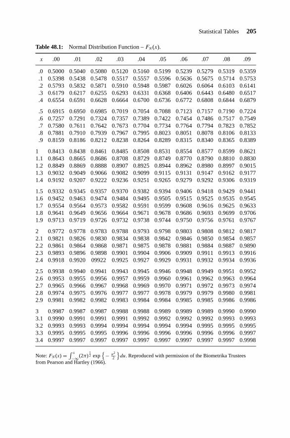
Statistical Tables 205
Table 48.1: Normal Distribution Function – FN (x).
x .00 .01 .02 .03 .04 .05 .06 .07 .08 .09
.0 0.5000 0.5040 0.5080 0.5120 0.5160 0.5199 0.5239 0.5279 0.5319 0.5359
.1 0.5398 0.5438 0.5478 0.5517 0.5557 0.5596 0.5636 0.5675 0.5714 0.5753
.2 0.5793 0.5832 0.5871 0.5910 0.5948 0.5987 0.6026 0.6064 0.6103 0.6141
.3 0.6179 0.6217 0.6255 0.6293 0.6331 0.6368 0.6406 0.6443 0.6480 0.6517
.4 0.6554 0.6591 0.6628 0.6664 0.6700 0.6736 0.6772 0.6808 0.6844 0.6879
.5 0.6915 0.6950 0.6985 0.7019 0.7054 0.7088 0.7123 0.7157 0.7190 0.7224
.6 0.7257 0.7291 0.7324 0.7357 0.7389 0.7422 0.7454 0.7486 0.7517 0.7549
.7 0.7580 0.7611 0.7642 0.7673 0.7704 0.7734 0.7764 0.7794 0.7823 0.7852
.8 0.7881 0.7910 0.7939 0.7967 0.7995 0.8023 0.8051 0.8078 0.8106 0.8133
.9 0.8159 0.8186 0.8212 0.8238 0.8264 0.8289 0.8315 0.8340 0.8365 0.8389
1 0.8413 0.8438 0.8461 0.8485 0.8508 0.8531 0.8554 0.8577 0.8599 0.86211.1 0.8643 0.8665 0.8686 0.8708 0.8729 0.8749 0.8770 0.8790 0.8810 0.88301.2 0.8849 0.8869 0.8888 0.8907 0.8925 0.8944 0.8962 0.8980 0.8997 0.90151.3 0.9032 0.9049 0.9066 0.9082 0.9099 0.9115 0.9131 0.9147 0.9162 0.91771.4 0.9192 0.9207 0.9222 0.9236 0.9251 0.9265 0.9279 0.9292 0.9306 0.9319
1.5 0.9332 0.9345 0.9357 0.9370 0.9382 0.9394 0.9406 0.9418 0.9429 0.94411.6 0.9452 0.9463 0.9474 0.9484 0.9495 0.9505 0.9515 0.9525 0.9535 0.95451.7 0.9554 0.9564 0.9573 0.9582 0.9591 0.9599 0.9608 0.9616 0.9625 0.96331.8 0.9641 0.9649 0.9656 0.9664 0.9671 0.9678 0.9686 0.9693 0.9699 0.97061.9 0.9713 0.9719 0.9726 0.9732 0.9738 0.9744 0.9750 0.9756 0.9761 0.9767
2 0.9772 0.9778 0.9783 0.9788 0.9793 0.9798 0.9803 0.9808 0.9812 0.98172.1 0.9821 0.9826 0.9830 0.9834 0.9838 0.9842 0.9846 0.9850 0.9854 0.98572.2 0.9861 0.9864 0.9868 0.9871 0.9875 0.9878 0.9881 0.9884 0.9887 0.98902.3 0.9893 0.9896 0.9898 0.9901 0.9904 0.9906 0.9909 0.9911 0.9913 0.99162.4 0.9918 0.9920 09922 0.9925 0.9927 0.9929 0.9931 0.9932 0.9934 0.9936
2.5 0.9938 0.9940 0.9941 0.9943 0.9945 0.9946 0.9948 0.9949 0.9951 0.99522.6 0.9953 0.9955 0.9956 0.9957 0.9959 0.9960 0.9961 0.9962 0.9963 0.99642.7 0.9965 0.9966 0.9967 0.9968 0.9969 0.9970 0.9971 0.9972 0.9973 0.99742.8 0.9974 0.9975 0.9976 0.9977 0.9977 0.9978 0.9979 0.9979 0.9980 0.99812.9 0.9981 0.9982 0.9982 0.9983 0.9984 0.9984 0.9985 0.9985 0.9986 0.9986
3 0.9987 0.9987 0.9987 0.9988 0.9988 0.9989 0.9989 0.9989 0.9990 0.99903.1 0.9990 0.9991 0.9991 0.9991 0.9992 0.9992 0.9992 0.9992 0.9993 0.99933.2 0.9993 0.9993 0.9994 0.9994 0.9994 0.9994 0.9994 0.9995 0.9995 0.99953.3 0.9995 0.9995 0.9995 0.9996 0.9996 0.9996 0.9996 0.9996 0.9996 0.99973.4 0.9997 0.9997 0.9997 0.9997 0.9997 0.9997 0.9997 0.9997 0.9997 0.9998
Note: FN (x) =∫ x
−∞(2π)12 exp
{− u2
2
}du. Reproduced with permission of the Biometrika Trustees
from Pearson and Hartley (1966).

206 Chapter 48 Statistical Tables
Table 48.2: Percentiles of the Chi-Squared χ2 : ν Distribution, G(l − α).
ν
∖1 − α 0.99 0.975 0.95 0.9 0.1 0.05 0.025 0.01
1 1.57088E-04 9.82069E-04 3.93214E-03 0.015791 2.70554 3.84146 5.02389 6.634902 0.020101 0.0506356 0.102587 0.210721 4.60517 5.99146 7.37776 9.210343 0.114832 0.215795 0.351846 0.584374 6.25139 7.81473 9.34840 11.34494 0.297109 0.484419 0.710723 1.063623 7.77944 9.48773 11.1433 13.2767
5 0.554298 0.831212 1.145476 1.61031 9.23636 11.0705 12.8325 15.08636 0.872090 1.23734 1.63538 2.20413 10.6446 12.5916 14.4494 16.81197 1.239042 1.68987 2.16735 2.83311 12.0170 14.0671 16.0128 18.47538 1.64650 2.17973 2.73264 3.48954 13.3616 15.5073 17.5345 20.09029 2.08790 2.70039 3.32511 4.16816 14.6837 16.9190 19.0228 21.6660
10 2.55821 3.24697 3.94030 4.86518 15.9872 18.3070 20.4832 23.209311 3.05348 3.81575 4.57481 5.57778 17.2750 19.6751 21.9200 24.725012 3.57057 4.40379 5.22603 6.30380 18.5493 21.0261 23.3367 26.217013 4.10692 5.00875 5.89186 7.04150 19.8119 22.3620 24.7356 27.688214 4.66043 5.62873 6.57063 7.78953 21.0641 23.6848 26.1189 29.1412
15 5.22935 6.26214 7.26094 8.54676 22.3071 24.9958 27.4884 30.577916 5.81221 6.90766 7.96165 9.31224 23.5418 26.2962 28.8454 31.999917 6.40776 7.56419 8.67176 10.0852 24.7690 27.5871 30.1910 33.408718 7.01491 8.23075 9.39046 10.8649 25.9894 28.8693 31.5264 34.805319 7.63273 8.90652 10.1170 11.6509 27.2036 30.1435 32.8523 36.1909
20 8.26040 9.59078 10.8508 12.4426 28.4120 31.4104 34.1696 37.566221 8.89720 10.2829 11.5913 13.2396 29.6151 32.6706 35.4789 38.932222 9.54249 10.9823 12.3380 14.0415 30.8133 33.9244 36.7807 40.289423 10.1957 11.6886 13.0905 14.8480 32.0069 35.1725 38.0756 41.638424 10.8564 12.4012 13.8484 15.6587 33.1962 36.4150 39.3641 42.9798
25 11.5240 13.1197 14.6114 16.4734 34.3816 37.6525 40.6465 44.314126 12.1981 13.8439 15.3792 17.2919 35.5632 38.8851 41.9232 45.641727 12.8785 14.5734 16.1514 18.1139 36.7412 40.1133 43.1945 46.962928 13.5647 15.3079 16.9279 18.9392 37.9159 41.3371 44.4608 48.278229 14.2565 16.0471 17.7084 19.7677 39.0875 42.5570 45.7223 49.5879
30 14.9535 16.7908 18.4927 20.5992 40.2560 43.7730 46.9792 50.892240 22.1643 24.4330 26.5093 29.0505 51.8051 55.7585 59.3417 63.690750 29.7067 32.3574 34.7643 37.6886 63.1671 67.5048 71.4202 76.153960 37.4849 40.4817 43.1880 46.4589 74.3970 79.0819 83.2977 88.3794
70 45.4417 48.7576 51.7393 55.3289 85.5270 90.5312 95.0232 100.42580 53.5401 57.1532 60.3915 64.2778 96.5782 101.879 106.629 112.32990 61.7541 65.6466 69.1260 73.2911 107.565 113.145 118.136 124.116
100 70.0649 74.2219 77.9295 82.3581 118.498 124.342 129.561 135.807
Note: Pr[χ2 : ν > G(l − α)] = α. Reproduced with permission of the Biometrika Trustees from Pearsonand Hartley (1966).

Statistical Tables 207
Table 48.3: Percentiles of the F : ν, ω DistributionUpper 5% points = G(0.95)
ω
∖ν
1 2 3 4 5 6 7 8 9 10 12 15 20 24 30 40 60 120 ∞1 161.4 199.5 215.7 224.6 230.2 234.0 236.8 238.9 240.5 241.9 243.9 245.9 248.0 249.1 250.1 251.1 252.2 253.3 254.32 18.51 19.00 19.16 19.25 19.30 19.33 19.35 19.37 19.38 19.40 19.41 19.43 19.45 19.45 19.46 19.47 19.48 19.49 19.503 10.13 9.55 9.28 9.12 9.01 8.94 8.89 8.85 8.81 8.79 8.74 8.70 8.66 8.64 8.62 8.59 8.57 8.55 8.534 7.71 6.94 6.59 6.39 6.26 6.16 6.09 6.04 6.00 5.96 5.91 5.86 5.80 5.77 5.75 5.72 5.69 5.66 5.63
5 6.61 5.79 5.41 5.19 5.05 4.95 4.88 4.82 4.77 4.74 4.68 4.62 4.56 4.53 4.50 4.46 4.43 4.40 4.366 5.99 5.14 4.76 4.53 4.39 4.28 4.21 4.15 4.10 4.06 4.00 3.94 3.87 3.84 3.81 3.77 3.74 3.70 3.677 5.59 4.74 4.35 4.12 3.97 3.87 3.79 3.73 3.68 3.64 3.57 3.51 3.44 3.41 3.38 3.34 3.30 3.27 3.238 5.32 4.46 4.07 3.84 3.69 3.58 3.50 3.44 3.39 3.35 3.28 3.22 3.15 3.12 3.08 3.04 3.01 2.97 2.939 5.12 4.26 3.86 3.63 3.48 3.37 3.29 3.23 3.18 3.14 3.07 3.01 2.94 2.90 2.86 2.83 2.79 2.75 2.71
10 4.96 4.10 3.71 3.48 3.33 3.22 3.14 3.07 3.02 2.98 2.91 2.85 2.77 2.74 2.70 2.66 2.62 2.58 2.5411 4.84 3.98 3.59 3.36 3.20 3.09 3.01 2.95 2.90 2.85 2.79 2.72 2.65 2.61 2.57 2.53 2.49 2.45 2.4012 4.75 3.89 3.49 3.26 3.11 3.00 2.91 2.85 2.80 2.75 2.69 2.62 2.54 2.51 2.47 2.43 2.38 2.34 2.3013 4.67 3.81 3.41 3.18 3.03 2.92 2.83 2.77 2.71 2.67 2.60 2.53 2.46 2.42 2.38 2.34 2.30 2.25 2.2114 4.60 3.74 3.34 3.11 2.96 2.85 2.76 2.70 2.65 2.60 2.53 2.46 2.39 2.35 2.31 2.27 2.22 2.18 2.13
15 4.54 3.68 3.29 3.06 2.90 2.79 2.71 2.64 2.59 2.54 2.48 2.40 2.33 2.29 2.25 2.20 2.16 2.11 2.0716 4.49 3.63 3.24 3.01 2.85 2.74 2.66 2.59 2.54 2.49 2.42 2.35 2.28 2.24 2.19 2.15 2.11 2.06 2.0117 4.45 3.59 3.20 2.96 2.81 2.70 2.61 2.55 2.49 2.45 2.38 2.31 2.23 2.19 2.15 2.10 2.06 2.01 1.9618 4.41 3.55 3.16 2.93 2.77 2.66 2.58 2.51 2.46 2.41 2.34 2.27 2.19 2.15 2.11 2.06 2.02 1.97 1.9219 4.38 3.52 3.13 2.90 2.74 2.63 2.54 2.48 2.42 2.38 2.31 2.23 2.16 2.11 2.07 2.03 1.98 1.93 1.88
20 4.35 3.49 3.10 2.87 2.71 2.60 2.51 2.45 2.39 2.35 2.28 2.20 2.12 2.08 2.04 1.99 1.95 1.90 1.8421 4.32 3.47 3.07 2.84 2.68 2.57 2.49 2.42 2.37 2.32 2.25 2.18 2.10 2.05 2.01 1.96 1.92 1.87 1.8122 4.30 3.44 3.05 2.82 2.66 2.55 2.46 2.40 2.34 2.30 2.23 2.15 2.07 2.03 1.98 1.94 1.89 1.84 1.7823 4.28 3.42 3.03 2.80 2.64 2.53 2.44 2.37 2.32 2.27 2.20 2.13 2.05 2.01 1.96 1.91 1.86 1.81 1.7624 4.26 3.40 3.01 2.78 2.62 2.51 2.42 2.36 2.30 2.25 2.18 2.11 2.03 1.98 1.94 1.89 1.84 1.79 1.73
25 4.24 3.39 2.99 2.76 2.60 2.49 2.40 2.34 2.28 2.24 2.16 2.09 2.01 1.96 1.92 1.87 1.82 1.77 1.7126 4.23 3.37 2.98 2.74 2.59 2.47 2.39 2.32 2.27 2.22 2.15 2.07 1.99 1.95 1.90 1.85 1.80 1.75 1.6927 4.21 3.35 2.96 2.73 2.57 2.46 2.37 2.31 2.25 2.20 2.13 2.06 1.97 1.93 1.88 1.84 1.79 1.73 1.6728 4.20 3.34 2.95 2.71 2.56 2.45 2.36 2.29 2.24 2.19 2.12 2.04 1.96 1.91 1.87 1.82 1.77 1.71 1.6529 4.18 3.33 2.93 2.70 2.55 2.43 2.35 2.28 2.22 2.18 2.10 2.03 1.94 1.90 1.85 1.81 1.75 1.70 1.64
30 4.17 3.32 2.92 2.69 2.53 2.42 2.33 2.27 2.21 2.16 2.09 2.01 1.93 1.89 1.84 1.79 1.74 1.68 1.6240 408 3.23 2.84 2.61 2.45 234 2.25 2.18 2.12 2.08 2.00 1.92 1.84 1.79 1.74 1.69 1.64 1.58 1.5160 4.00 3.15 2.76 2.53 2.37 2.25 2.17 2.10 2.04 1.99 1.92 1.84 1.75 1.70 1.65 1.59 1.53 1.47 1.39
120 3.92 3.07 2.68 2.45 2.29 2.17 2.09 2.02 1.96 1.91 1.83 1.75 1.66 1.61 1.55 1.50 1.43 1.35 1.25∞ 3.84 3.00 2.60 2.37 2.21 2.10 2.01 1.94 1.88 1.83 1.75 1.67 1.57 1.52 1.46 1.39 1.32 1.22 1.01
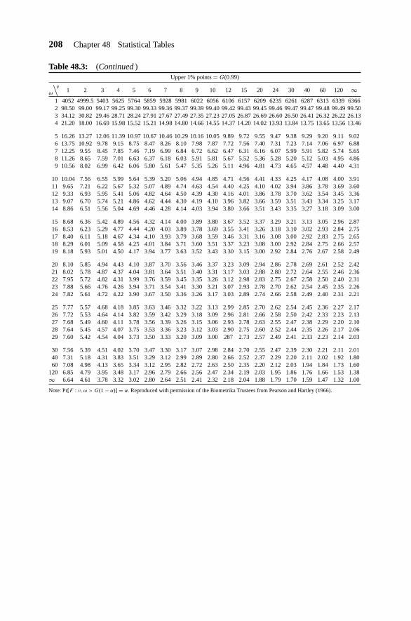
208 Chapter 48 Statistical Tables
Table 48.3: (Continued )Upper 1% points = G(0.99)
ω
∖ν
1 2 3 4 5 6 7 8 9 10 12 15 20 24 30 40 60 120 ∞1 4052 4999.5 5403 5625 5764 5859 5928 5981 6022 6056 6106 6157 6209 6235 6261 6287 6313 6339 63662 98.50 99.00 99.17 99.25 99.30 99.33 99.36 99.37 99.39 99.40 99.42 99.43 99.45 99.46 99.47 99.47 99.48 99.49 99.503 34.12 30.82 29.46 28.71 28.24 27.91 27.67 27.49 27.35 27.23 27.05 26.87 26.69 26.60 26.50 26.41 26.32 26.22 26.134 21.20 18.00 16.69 15.98 15.52 15.21 14.98 14.80 14.66 14.55 14.37 14.20 14.02 13.93 13.84 13.75 13.65 13.56 13.46
5 16.26 13.27 12.06 11.39 10.97 10.67 10.46 10.29 10.16 10.05 9.89 9.72 9.55 9.47 9.38 9.29 9.20 9.11 9.026 13.75 10.92 9.78 9.15 8.75 8.47 8.26 8.10 7.98 7.87 7.72 7.56 7.40 7.31 7.23 7.14 7.06 6.97 6.887 12.25 9.55 8.45 7.85 7.46 7.19 6.99 6.84 6.72 6.62 6.47 6.31 6.16 6.07 5.99 5.91 5.82 5.74 5.658 11.26 8.65 7.59 7.01 6.63 6.37 6.18 6.03 5.91 5.81 5.67 5.52 5.36 5.28 5.20 5.12 5.03 4.95 4.869 10.56 8.02 6.99 6.42 6.06 5.80 5.61 5.47 5.35 5.26 5.11 4.96 4.81 4.73 4.65 4.57 4.48 4.40 4.31
10 10.04 7.56 6.55 5.99 5.64 5.39 5.20 5.06 4.94 4.85 4.71 4.56 4.41 4.33 4.25 4.17 4.08 4.00 3.9111 9.65 7.21 6.22 5.67 5.32 5.07 4.89 4.74 4.63 4.54 4.40 4.25 4.10 4.02 3.94 3.86 3.78 3.69 3.6012 9.33 6.93 5.95 5.41 5.06 4.82 4.64 4.50 4.39 4.30 4.16 4.01 3.86 3.78 3.70 3.62 3.54 3.45 3.3613 9.07 6.70 5.74 5.21 4.86 4.62 4.44 4.30 4.19 4.10 3.96 3.82 3.66 3.59 3.51 3.43 3.34 3.25 3.1714 8.86 6.51 5.56 5.04 4.69 4.46 4.28 4.14 4.03 3.94 3.80 3.66 3.51 3.43 3.35 3.27 3.18 3.09 3.00
15 8.68 6.36 5.42 4.89 4.56 4.32 4.14 4.00 3.89 3.80 3.67 3.52 3.37 3.29 3.21 3.13 3.05 2.96 2.8716 8.53 6.23 5.29 4.77 4.44 4.20 4.03 3.89 3.78 3.69 3.55 3.41 3.26 3.18 3.10 3.02 2.93 2.84 2.7517 8.40 6.11 5.18 4.67 4.34 4.10 3.93 3.79 3.68 3.59 3.46 3.31 3.16 3.08 3.00 2.92 2.83 2.75 2.6518 8.29 6.01 5.09 4.58 4.25 4.01 3.84 3.71 3.60 3.51 3.37 3.23 3.08 3.00 2.92 2.84 2.75 2.66 2.5719 8.18 5.93 5.01 4.50 4.17 3.94 3.77 3.63 3.52 3.43 3.30 3.15 3.00 2.92 2.84 2.76 2.67 2.58 2.49
20 8.10 5.85 4.94 4.43 4.10 3.87 3.70 3.56 3.46 3.37 3.23 3.09 2.94 2.86 2.78 2.69 2.61 2.52 2.4221 8.02 5.78 4.87 4.37 4.04 3.81 3.64 3.51 3.40 3.31 3.17 3.03 2.88 2.80 2.72 2.64 2.55 2.46 2.3622 7.95 5.72 4.82 4.31 3.99 3.76 3.59 3.45 3.35 3.26 3.12 2.98 2.83 2.75 2.67 2.58 2.50 2.40 2.3123 7.88 5.66 4.76 4.26 3.94 3.71 3.54 3.41 3.30 3.21 3.07 2.93 2.78 2.70 2.62 2.54 2.45 2.35 2.2624 7.82 5.61 4.72 4.22 3.90 3.67 3.50 3.36 3.26 3.17 3.03 2.89 2.74 2.66 2.58 2.49 2.40 2.31 2.21
25 7.77 5.57 4.68 4.18 3.85 3.63 3.46 3.32 3.22 3.13 2.99 2.85 2.70 2.62 2.54 2.45 2.36 2.27 2.1726 7.72 5.53 4.64 4.14 3.82 3.59 3.42 3.29 3.18 3.09 2.96 2.81 2.66 2.58 2.50 2.42 2.33 2.23 2.1327 7.68 5.49 4.60 4.11 3.78 3.56 3.39 3.26 3.15 3.06 2.93 2.78 2.63 2.55 2.47 2.38 2.29 2.20 2.1028 7.64 5.45 4.57 4.07 3.75 3.53 3.36 3.23 3.12 3.03 2.90 2.75 2.60 2.52 2.44 2.35 2.26 2.17 2.0629 7.60 5.42 4.54 4.04 3.73 3.50 3.33 3.20 3.09 3.00 287 2.73 2.57 2.49 2.41 2.33 2.23 2.14 2.03
30 7.56 5.39 4.51 4.02 3.70 3.47 3.30 3.17 3.07 2.98 2.84 2.70 2.55 2.47 2.39 2.30 2.21 2.11 2.0140 7.31 5.18 4.31 3.83 3.51 3.29 3.12 2.99 2.89 2.80 2.66 2.52 2.37 2.29 2.20 2.11 2.02 1.92 1.8060 7.08 4.98 4.13 3.65 3.34 3.12 2.95 2.82 2.72 2.63 2.50 2.35 2.20 2.12 2.03 1.94 1.84 1.73 1.60
120 6.85 4.79 3.95 3.48 3.17 2.96 2.79 2.66 2.56 2.47 2.34 2.19 2.03 1.95 1.86 1.76 1.66 1.53 1.38∞ 6.64 4.61 3.78 3.32 3.02 2.80 2.64 2.51 2.41 2.32 2.18 2.04 1.88 1.79 1.70 1.59 1.47 1.32 1.00
Note: Pr[F : ν, ω > G(1 − α)] = α. Reproduced with permission of the Biometrika Trustees from Pearson and Hartley (1966).
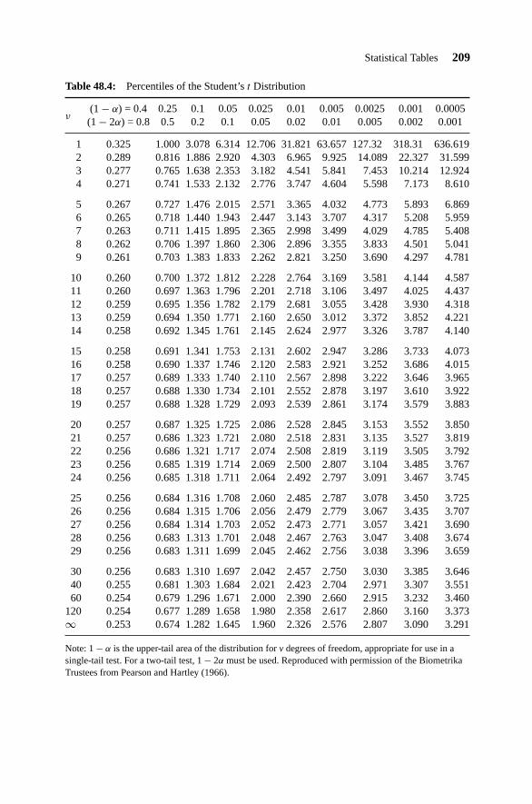
Statistical Tables 209
Table 48.4: Percentiles of the Student’s t Distribution
(1 − α) = 0.4 0.25 0.1 0.05 0.025 0.01 0.005 0.0025 0.001 0.0005(1 − 2α) = 0.8 0.5 0.2 0.1 0.05 0.02 0.01 0.005 0.002 0.001ν
1 0.325 1.000 3.078 6.314 12.706 31.821 63.657 127.32 318.31 636.6192 0.289 0.816 1.886 2.920 4.303 6.965 9.925 14.089 22.327 31.5993 0.277 0.765 1.638 2.353 3.182 4.541 5.841 7.453 10.214 12.9244 0.271 0.741 1.533 2.132 2.776 3.747 4.604 5.598 7.173 8.610
5 0.267 0.727 1.476 2.015 2.571 3.365 4.032 4.773 5.893 6.8696 0.265 0.718 1.440 1.943 2.447 3.143 3.707 4.317 5.208 5.9597 0.263 0.711 1.415 1.895 2.365 2.998 3.499 4.029 4.785 5.4088 0.262 0.706 1.397 1.860 2.306 2.896 3.355 3.833 4.501 5.0419 0.261 0.703 1.383 1.833 2.262 2.821 3.250 3.690 4.297 4.781
10 0.260 0.700 1.372 1.812 2.228 2.764 3.169 3.581 4.144 4.58711 0.260 0.697 1.363 1.796 2.201 2.718 3.106 3.497 4.025 4.43712 0.259 0.695 1.356 1.782 2.179 2.681 3.055 3.428 3.930 4.31813 0.259 0.694 1.350 1.771 2.160 2.650 3.012 3.372 3.852 4.22114 0.258 0.692 1.345 1.761 2.145 2.624 2.977 3.326 3.787 4.140
15 0.258 0.691 1.341 1.753 2.131 2.602 2.947 3.286 3.733 4.07316 0.258 0.690 1.337 1.746 2.120 2.583 2.921 3.252 3.686 4.01517 0.257 0.689 1.333 1.740 2.110 2.567 2.898 3.222 3.646 3.96518 0.257 0.688 1.330 1.734 2.101 2.552 2.878 3.197 3.610 3.92219 0.257 0.688 1.328 1.729 2.093 2.539 2.861 3.174 3.579 3.883
20 0.257 0.687 1.325 1.725 2.086 2.528 2.845 3.153 3.552 3.85021 0.257 0.686 1.323 1.721 2.080 2.518 2.831 3.135 3.527 3.81922 0.256 0.686 1.321 1.717 2.074 2.508 2.819 3.119 3.505 3.79223 0.256 0.685 1.319 1.714 2.069 2.500 2.807 3.104 3.485 3.76724 0.256 0.685 1.318 1.711 2.064 2.492 2.797 3.091 3.467 3.745
25 0.256 0.684 1.316 1.708 2.060 2.485 2.787 3.078 3.450 3.72526 0.256 0.684 1.315 1.706 2.056 2.479 2.779 3.067 3.435 3.70727 0.256 0.684 1.314 1.703 2.052 2.473 2.771 3.057 3.421 3.69028 0.256 0.683 1.313 1.701 2.048 2.467 2.763 3.047 3.408 3.67429 0.256 0.683 1.311 1.699 2.045 2.462 2.756 3.038 3.396 3.659
30 0.256 0.683 1.310 1.697 2.042 2.457 2.750 3.030 3.385 3.64640 0.255 0.681 1.303 1.684 2.021 2.423 2.704 2.971 3.307 3.55160 0.254 0.679 1.296 1.671 2.000 2.390 2.660 2.915 3.232 3.460
120 0.254 0.677 1.289 1.658 1.980 2.358 2.617 2.860 3.160 3.373∞ 0.253 0.674 1.282 1.645 1.960 2.326 2.576 2.807 3.090 3.291
Note: 1 − α is the upper-tail area of the distribution for v degrees of freedom, appropriate for use in asingle-tail test. For a two-tail test, 1 − 2α must be used. Reproduced with permission of the BiometrikaTrustees from Pearson and Hartley (1966).

210 Chapter 48 Statistical Tables
Table 48.5: Partial Expectations for the Standard Normal Distribution
Partial expectation P(x) = ∫ ∞x
(u − x)f (u) du
When x < 3.0, use −x as an approximation for the partial expectation
x P(x) x P(x) x P(x)
−2.9 2.9005 −0.9 1.0004 1.1 0.0686−2.8 2.8008 −0.8 0.9202 1.2 0.0561−2.7 2.7011 −0.7 0.8429 1.3 0.0455−2.6 2.6015 −0.6 0.7687 1.4 0.0367−2.5 2.5020 −0.5 0.6987 1.5 0.0293−2.4 2.4027 −0.4 0.6304 1.6 0.0232−2.3 2.3037 −0.3 0.5668 1.7 0.0183−2.2 2.2049 −0.2 0.5069 1.8 0.0143−2.1 2.1065 −0.1 0.4509 1.9 0.0111−2.0 2.0085 0.0 0.3989 2.0 0.0085−1.9 1.9111 0.1 0.3509 2.1 0.0065−1.8 1.8143 0.2 0.3069 2.2 0.0049−1.7 1.7183 0.3 0.2668 2.3 0.0037−1.6 1.6232 0.4 0.2304 2.4 0.0027−1.5 1.5293 0.5 0.1978 2.5 0.0020−1.4 1.4367 0.6 0.1687 2.6 0.0015−1.3 1.3455 0.7 0.1429 2.7 0.0011−1.2 1.2561 0.8 0.1202 2.8 0.0008−1.1 1.1686 0.9 0.1004 2.9 0.0005−1.0 1.0833 1.0 0.0833 3.0 0.0004

Bibliography
Azzalini, A., A Class of Distributions Which Includes the Normal Ones, Scandinavian Journal of Statis-tics, 12, 2, 171–178 (1985).
Bartlett, H. J. G., and Hastings, N. A. J., Improved Reliability Estimates for Samples ContainingSuspensions, Journal of Quality in Maintenance Engineering, 4, 107–114 (1998).
Box, G. E. P., Jenkins, G. M., and Reinsel, G. C., Time Series Analysis: Forecasting and Control, 4thed., Wiley (2008).
Casella, G., and Berger, R. L., Statistical Inference, 2nd ed., Thomson, (2002).Cooper, R., Introduction to Queuing Theory, 2nd ed., North-Holland, (1981).Cox, D. R., Principles of Statistical Inference, Cambridge, (2006).D’Agostino, R. B., and Stephens, M. A., Goodness of Fit Techniques, Marcel Dekker (1986).Fernandez, C., and Steel, M. F. J., On Bayesian Modeling of Fat Tails and Skewness, Journal of the
American Statistical Association, 93, 359–371 (1998).Fruhwirth-Schnatter, S., Finite Mixture and Markov Switching Models, Springer (2006).Hall, A. R., Generalized Method of Moments, Oxford University Press (2005).Hamilton, J. D., Time Series Analysis, Princeton University Press (1994).Johnson, N. L., and Kotz, S. Distributions in Statistics: Continuous Multivariate Distributions, Wiley
(1972).Johnson, N. L., and Kotz, S., Urn Models and Their Application, an Approach to Modern Discrete
Probability Theory, Wiley (1977).Johnson, N. L., and Kotz, S., Developments in Discrete Distributions, 1969–1980. International Statis-
tical Review, 50, 70–101 (1982).Johnson, N. L., Kotz, S., and Balakrishnan, N., Continuous Univariate Distributions, 2nd ed. (2 vols.),
Wiley (1994).Johnson, N. L., Kotz, S., and Kemp, A. W., Univariate Discrete Distributions, 3rd ed., Wiley (2005).Johnston, J., DiNardo, J., Econometric Methods, 4th ed., McGraw-Hill (1997).Kendall, D., Some Problems in the Theory of Queues, Journal of the Royal Statistical Society Series B,
13, 151–185, (1951).Kotz, S., and Johnson, N. L., Encyclopedia of Statistical Sciences, Volumes 1–9 and supplement, Wiley
(1982–1989).Lee, A., Applied Queuing Theory, St Martins Press, (1966).Lye, J., and Martin, V. L., Robust Estimation, Nonnormalities, and Generalized Exponential Distributions,
Journal of the American Statistical Association, 88, No. 421, 261–267 (1993).Mardia, K. V., Statistics of Directional Data, Academic Press (1972).Marriot, F. H. C., A Dictionary of Statistical Terms, 5th ed., Wiley, (1990).
Statistical Distributions, Fourth Edition, by Catherine Forbes, Merran Evans, Nicholas Hastings,and Brian PeacockCopyright © 2011 John Wiley & Sons, Inc.
211

212 Bibliography
McCullagh, P., and Nelder, J. A., Generalised Linear Models, Chapman and Hall (1989).Nadarajah, A. and Kotz, S., Skewed Distributions Generated by the Normal Kernal, Statistics and
Probability Letters, 65, 269–277 (2003).O’Hagan, A. and Leonard, T., Bayes Estimation Subject to Uncertainty About Parameter Constraints,
Biometrika, 63, 2, 201–203 (1976).Patel, J. K., Kapadia, C. H., and Owen, D. B., Handbook of Statistical Distributions, Marcel Dekker
(1976).Patil, G. P., Boswell, M. T., and Ratnaparkhi, M. V., Dictionary and Classified Bibliography of
Statistical Distributions in Scientific Work: Vol. 1. Discrete Models (with S. W. Joshi); Vol. 2. ContinuousUnivariate Models; Vol. 3. Multivariate Models (with J. J. J. Roux), International Cooperative PublishingHouse (1984).
Pearson, E. S., and Hartley, H. O., eds., Biometrika Tables for Statisticians, Vol. 1, 3rd ed., CambridgeUniversity Press (1966).
Pearson, K. ed., Tables of Incomplete Beta Functions, 2nd ed., Cambridge University Press (1968).Robert, C. P., The Bayesian Choice: From Decision-Theoretic Foundations to Computational Implemen-
tation, 2nd ed., Springer (2007).Stuart, A., and Ord, J. K., Kendall’s Advanced Theory of Statistics, Vol. I, Distribution Theory, 6th ed.,
Hodder Arnold (1994).Winston, W.L., Operations Research, Brooks/Cole-Thompson Learning, (2004).


