Statistical Color Models with Application to Skin Detection with EM Training

Anthony Dotterer

3-1-2006

Introduction

Jones and Rehg develop two Gaussian mixture models (GMM) representing color of skin and not-skin in [1]. However, these models are quite generic; since they were trained using many different images from the web under arbitrary illumination conditions. This paper attempts to specialize these models to a single person with a constant background and constant illumination. To achieve this goal, Expectation Maximization (EM) is used on a set of training images to fine tune the Gaussian mixture models.

Setup

In order to perform EM, a Gaussian mixture model must be initialized. The GMMs derived in [1] are used from the code provided by Dr. Collins. There are 32 models, where 16 are skin matching models and the other 16 are non-skin, background models. The following figures show some input, the skin mask output, and the image mask output.

Illustration 1: Input picture 1

Illustration 2: Skin mask of picture 1

Illustration 3: Image masked for picture 1

The following table contains the parameters of the GMMs in [1].

Model Red Mean

Green Mean

Blue Mean

Red Variance

Green Variance

Blue Variance

Weight

1 73.53 29.94 17.76 765.40 121.44 112.80 0.02942 249.71 233.94 217.49 39.94 154.44 396.05 0.03313 161.68 116.25 96.95 291.03 60.48 162.85 0.06544 186.07 136.62 114.40 274.95 64.60 198.27 0.07565 189.26 98.37 51.18 633.18 222.40 250.69 0.05546 247.00 152.20 90.84 65.23 691.53 609.92 0.03147 150.10 72.66 37.76 408.63 200.77 257.57 0.04548 206.85 171.09 156.34 530.08 155.08 572.79 0.04699 212.78 152.82 120.04 160.57 84.52 243.90 0.0956

10 234.87 175.43 138.94 163.80 121.57 279.22 0.076311 151.19 97.74 74.59 425.40 73.56 175.11 0.110012 120.52 77.55 59.82 330.45 70.34 151.82 0.067613 192.20 119.62 82.32 152.76 92.14 259.15 0.075514 214.29 136.08 87.24 204.90 140.17 270.19 0.050015 99.57 54.33 38.06 448.13 90.18 151.29 0.066716 238.88 203.08 176.91 178.38 156.27 404.99 0.0749

Skin GMM

Model Red Mean

Green Mean

Blue Mean

Red Variance

Green Variance

Blue Variance

Weight

1 254.37 254.41 253.82 2.77 2.81 5.46 0.06372 9.39 8.09 8.52 46.84 33.59 32.48 0.05163 96.57 96.95 91.53 280.69 156.79 436.58 0.08644 160.44 162.49 159.06 355.98 115.89 591.24 0.06365 74.98 63.23 46.33 414.84 245.95 361.27 0.07476 121.83 60.88 18.31 2502.24 1383.53 237.18 0.03657 202.18 154.88 91.04 957.42 1766.94 1582.52 0.03498 193.06 201.93 206.55 562.88 190.23 447.28 0.06499 51.88 57.14 61.55 344.11 191.77 433.40 0.0656

10 30.88 26.84 25.32 222.07 118.65 182.41 0.118911 44.97 85.96 131.95 651.32 840.52 963.67 0.0362

Model Red Mean

Green Mean

Blue Mean

Red Variance

Green Variance

Blue Variance

Weight

12 236.02 236.27 230.70 225.03 117.29 331.95 0.084913 207.86 191.2 164.12 494.04 237.69 533.52 0.036814 99.83 148.11 188.17 955.88 654.95 916.70 0.038915 135.06 131.92 123.10 350.35 130.30 388.43 0.094316 135.96 103.89 66.88 806.44 642.20 350.36 0.0477

Non-skin GMM

These models in [1] were applied using the Matlab code in Appendix A provided by Dr. Collins.

In order to apply EM to a picture, the mixture models need to be combined to correctly train to the person's skin and the background of the pictures. To combine the GMMs, the sum of both of the GMMs' weights must equal 1. Therefore, the weights of both GMMs are divided by 2.

Basic EM Implementation

To initialize the EM algorithm, an array of parameters is constructed. This array grows with each iteration and contains each GMMs' means, variances, and weights at each iteration of the EM algorithm.

The EM algorithm starts with the expectation step or E-step. This step computes the probabilities of all data points for each Gaussian model. Next, all of these probabilities are summed up. Finally, each of the calculated probabilities for each models are normalized with the previously calculated sum.

The next step of is of the algorithm is the maximization step or M-step. In this step, the mean, variance, and weight of each GMM is maximized for the data set. First

Formula 1: Parameter Set extracted from [2]

Formula 2: The sum of the probabilities for each class from [2]

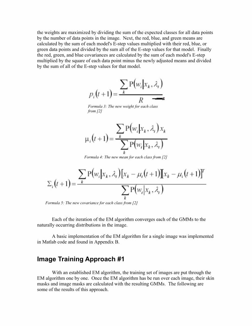
the weights are maximized by dividing the sum of the expected classes for all data points by the number of data points in the image. Next, the red, blue, and green means are calculated by the sum of each model's E-step values multiplied with their red, blue, or green data points and divided by the sum all of the E-step values for that model. Finally the red, green, and blue covariances are calculated by the sum of each model's E-step multiplied by the square of each data point minus the newly adjusted means and divided by the sum of all of the E-step values for that model.

Each of the iteration of the EM algorithm converges each of the GMMs to the naturally occurring distributions in the image.

A basic implementation of the EM algorithm for a single image was implemented in Matlab code and found in Appendix B.

Image Training Approach #1

With an established EM algorithm, the training set of images are put through the EM algorithm one by one. Once the EM algorithm has be run over each image, their skin masks and image masks are calculated with the resulting GMMs. The following are some of the results of this approach.

Formula 3: The new weight for each class from [2]

Formula 4: The new mean for each class from [2]

Formula 5: The new covariance for each class from [2]

Illustration 4: Input picture 2

Illustration 5: Skin mask from approach 1

Illustration 6: Image masked for picture 6

The following tables contain the GMMs after this approach.

Models Red Mean

Green Mean

Blue Mean

Red Variance

Green Variance

Blue Variance

Weight

1 37.4484 32.5658 34.1843 13.8999 4.3041 6.2758 0.07232 182.0000 185.0000 192.0000 0.0000 0.0000 0.0000 0.00003 94.7552 99.6847 111.0957 17.2699 19.5284 28.4164 0.12124 142.9789 145.5472 153.2264 16.9915 11.5471 17.9825 0.01345 120.9929 80.2765 74.3183 36.5524 17.6171 5.0302 0.02536 182.0000 188.0000 186.0000 0.0000 0.0000 0.0000 0.00007 112.4719 81.5838 75.4216 32.0925 9.9314 5.4775 0.09268 168.4660 171.4826 178.6172 8.2754 3.6815 3.2656 0.07869 163.5939 166.8673 174.5367 4.8418 1.2531 1.9210 0.0231

10 179.0000 181.0000 180.0000 0.0000 0.0000 0.0000 0.000011 131.5429 91.3794 85.1058 80.9489 37.2305 30.9587 0.431712 103.1082 72.8879 69.4870 87.9763 13.7888 9.9340 0.083713 135.0000 96.0000 89.0000 0.0000 0.0000 0.0000 0.000014 142.6915 144.9823 152.0000 18.8445 7.9394 0.0000 0.001915 76.7001 57.6445 58.2287 232.1433 9.9674 20.2618 0.056216 181.0000 185.0000 188.0000 0.0000 0.0000 0.0000 0.0000

Skin GMM

Models Red Mean

Green Mean

Blue Mean

Red Variance

Green Variance

Blue Variance

Weight

1 254.3700 254.4100 253.8200 2.7700 2.8100 5.4600 0.00002 26.0199 22.7637 23.9363 2.3893 2.0352 2.0911 0.05643 85.5143 89.4215 97.6160 12.3674 9.2640 17.9022 0.09054 159.2924 162.7913 170.4675 9.7654 3.8964 5.4984 0.02795 90.3027 65.5843 62.7222 60.4085 7.2927 9.6805 0.03716 50.4974 40.3170 42.1664 91.5191 7.9992 11.1414 0.03947 156.4721 158.3457 164.5596 6.0494 1.1693 3.6613 0.00888 185.2112 184.5222 189.3651 12.6228 10.2581 8.7647 0.33409 65.4967 49.3106 50.3677 158.3785 9.3339 12.3695 0.0377

10 31.0593 27.3243 28.7598 4.8150 2.6862 3.2846 0.1108

Models Red Mean

Green Mean

Blue Mean

Red Variance

Green Variance

Blue Variance

Weight

11 76.8143 80.9796 88.3997 6.6987 6.0730 6.1805 0.035212 182.0000 188.0000 186.0000 0.0000 0.0000 0.0000 0.000013 175.6366 177.1109 183.1107 10.3601 3.4434 3.4622 0.147314 151.4817 153.8402 160.7890 9.5545 4.8666 11.1621 0.016415 123.6912 122.7599 131.2196 136.7536 112.7450 122.7393 0.029316 69.2796 70.0922 76.8519 47.5771 20.1546 23.0501 0.0294

Non-skin GMM

These tables show that the EM algorithm is working due to the contrast in the original variances versus the final variances as well as the differences in the models' weights. One thing to point out is the number of models that have a probability of 0 which effectively removes this model. Some models even have an almost 0 variance, meaning that they only models a pixel at their means although these only occur when their weights are almost 0.

This EM process was implemented in Matlab using the EM calculation function in Appendix D and the GMM applier in Appendix C.

This particular EM approach has a downfall. It biases on the last image. EM is meant to be run over the whole training set to encompass all of the different features that occur in all of the training images. The next section will describe an approach that attempts to remedy this problem.

Image Training Approach #2

This second approach to training the GMM algorithm with the EM algorithm is to run it over the entire training set. Unfortunately this approach creates a problem with memory limits, due the fact that the entire training set must be loaded into memory. Therefore, the training sets were limited to three images. The following figures are the results from training on the first three images.

Illustration 7: Input image 0

Illustration 8: Skin mask from approach 2

The following tables contain the GMMs after this approach.

Model Red Mean

Green Mean

Blue Mean

Red Variance

Green Variance

Blue Variance

Weight

1 44.7533 37.7986 37.6286 54.9015 8.4493 8.2369 0.05792 192.9774 195.0191 194.0191 0.0235 0.0209 0.0209 0.00003 111.5958 116.2774 119.0166 61.1048 58.4686 63.6481 0.04334 148.0359 149.1413 148.2574 40.6585 4.5243 4.9476 0.09845 118.1438 81.8271 73.7301 13.3746 6.1385 2.6059 0.00756 190.4370 191.8304 191.7016 2.6987 3.2964 5.7048 0.00007 106.3561 76.8091 68.2218 64.6643 19.3080 15.2999 0.00168 169.8269 171.1283 171.4325 11.5098 6.4394 11.7756 0.34779 165.1209 166.8360 166.9714 5.5512 2.9833 4.0836 0.0001

10 180.1756 180.4754 178.1448 1.6843 1.4019 3.7059 0.000111 123.5026 86.7994 77.1792 54.5835 16.9132 12.1807 0.097912 104.2707 75.4331 66.9675 62.0316 15.9075 14.0191 0.194513 141.1892 98.0875 89.2599 8.4821 7.1792 5.7496 0.0020

Illustration 9: Image masked from input 0

Model Red Mean

Green Mean

Blue Mean

Red Variance

Green Variance

Blue Variance

Weight

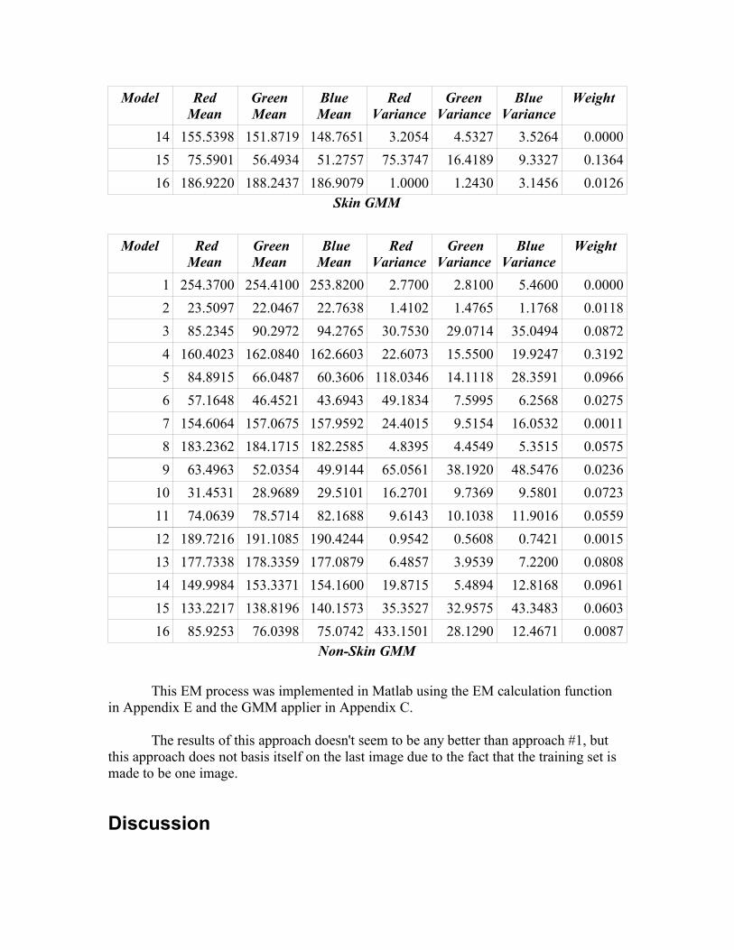
14 155.5398 151.8719 148.7651 3.2054 4.5327 3.5264 0.000015 75.5901 56.4934 51.2757 75.3747 16.4189 9.3327 0.136416 186.9220 188.2437 186.9079 1.0000 1.2430 3.1456 0.0126

Skin GMM

Model Red Mean

Green Mean

Blue Mean

Red Variance

Green Variance

Blue Variance

Weight

1 254.3700 254.4100 253.8200 2.7700 2.8100 5.4600 0.00002 23.5097 22.0467 22.7638 1.4102 1.4765 1.1768 0.01183 85.2345 90.2972 94.2765 30.7530 29.0714 35.0494 0.08724 160.4023 162.0840 162.6603 22.6073 15.5500 19.9247 0.31925 84.8915 66.0487 60.3606 118.0346 14.1118 28.3591 0.09666 57.1648 46.4521 43.6943 49.1834 7.5995 6.2568 0.02757 154.6064 157.0675 157.9592 24.4015 9.5154 16.0532 0.00118 183.2362 184.1715 182.2585 4.8395 4.4549 5.3515 0.05759 63.4963 52.0354 49.9144 65.0561 38.1920 48.5476 0.0236

10 31.4531 28.9689 29.5101 16.2701 9.7369 9.5801 0.072311 74.0639 78.5714 82.1688 9.6143 10.1038 11.9016 0.055912 189.7216 191.1085 190.4244 0.9542 0.5608 0.7421 0.001513 177.7338 178.3359 177.0879 6.4857 3.9539 7.2200 0.080814 149.9984 153.3371 154.1600 19.8715 5.4894 12.8168 0.096115 133.2217 138.8196 140.1573 35.3527 32.9575 43.3483 0.060316 85.9253 76.0398 75.0742 433.1501 28.1290 12.4671 0.0087

Non-Skin GMM

This EM process was implemented in Matlab using the EM calculation function in Appendix E and the GMM applier in Appendix C.

The results of this approach doesn't seem to be any better than approach #1, but this approach does not basis itself on the last image due to the fact that the training set is made to be one image.

Discussion

Both of the approaches to apply an EM algorithm to a training set seem to make the skin GMMs match more of the background and non-skin areas like hair and eyes. I think that this occurs because the skin GMMs need to be trained only to skin, and the non-skin GMMs need to be trained only to the background. Unfortunately, trying to identify the skin is the job of the algorithm. Thusly, we have the chicken and the egg situation. Only if a person was to 'cut' out the skin from the background, and then train each GMM set to the appropriate images would the results be anything great. It maybe possible to use the skin GMM to generically identify the person's skin, then using EM on the skin GMM for the masked image. With the EMed skin GMM, the training set would have its skin mask recalculated. Then with the new mask, the background GMMs could be EMed on the unmasked image area. Finally the trained skin GMM and non-skin GMM could be ran on the images to better find the person's skin.

References

[1] Michael J. Jones, James M. Rehg, "Statistical Color Models with Application to Skin Detection," cvpr, p. 1274, 1999 IEEE Computer Society Conference on Computer Vision and Pattern Recognition (CVPR'99) - Volume 1, 1999.

[2] Lecture notes on GMM and EM for CSE586, lectured by Dr. Robert Collins. Figures are cited in slides to Andrew W. Moore, Copyright © 2001

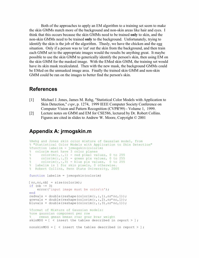
Appendix A: jrmogskin.m

%Rehg and Jones skin color mixture of Gaussian model, from% "Statistical Color Models with Application to Skin Detection"%function labelim = jrmogskin(colorim)% colorim must have 3 color planes% colorim(:,:,1) = red pixel values, 0 to 255% colorim(:,:,2) = green pix values, 0 to 255% colorim(:,:,3) = blue pix values, 0 to 255% labelim is 1 for skin pixels, 0 otherwise.% Robert Collins, Penn State University, 2005function labelim = jrmogskin(colorim)[nr,nc,nb] = size(colorim);if (nb ~= 3) error('input image must be color\n');endredvals = double(reshape(colorim(:,:,1),nr*nc,1));grevals = double(reshape(colorim(:,:,2),nr*nc,1));bluvals = double(reshape(colorim(:,:,3),nr*nc,1));%format of Mixture of Gaussian models:%one gaussian component per row% rmean gmean bmean rvar gvar bvar weightskinMOG = [ < insert the tables described in report > ];nonskinMOG = [ < insert the tables described in report > ];

skinscores = zeros(size(redvals));for i=1:size(skinMOG,1) p = skinMOG(i,:); tmp = ((redvals-p(1)).^2 / p(4) + (grevals-p(2)).^2 / p(5) + (bluvals-p(3)).^2 / p(6)); tmp = p(7) * exp(- tmp / 2) / ((2 * pi)^(3/2) * sqrt(p(4)*p(5)*p(6))); skinscores = skinscores + tmp;end

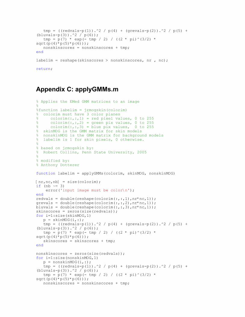
nonskinscores = zeros(size(redvals));for i=1:size(nonskinMOG,1) p = nonskinMOG(i,:); tmp = ((redvals-p(1)).^2 / p(4) + (grevals-p(2)).^2 / p(5) + (bluvals-p(3)).^2 / p(6)); tmp = p(7) * exp(- tmp / 2) / ((2 * pi)^(3/2) * sqrt(p(4)*p(5)*p(6))); nonskinscores = nonskinscores + tmp;endlabelim = reshape(skinscores > nonskinscores, nr , nc);return;

Appendix B: jrmogskinWithEM.m

%Rehg and Jones skin color mixture of Gaussian model, from% "Statistical Color Models with Application to Skin Detection"% with Anthony Dotterer's home brewed EM extension to train the% inital Gaussian Models to the passed picture for a better skin match.%%function labelim = jrmogskin(colorim)% colorim must have 3 color planes% colorim(:,:,1) = red pixel values, 0 to 255% colorim(:,:,2) = green pix values, 0 to 255% colorim(:,:,3) = blue pix values, 0 to 255% labelim is 1 for skin pixels, 0 otherwise.% Robert Collins, Penn State University, 2005%% added EM extension authored by% Anthony Dottererfunction labelim = jrmogskinWithEM(colorim)[nr,nc,nb] = size(colorim);if (nb ~= 3) error('input image must be color\n');endredvals = double(reshape(colorim(:,:,1),nr*nc,1));grevals = double(reshape(colorim(:,:,2),nr*nc,1));bluvals = double(reshape(colorim(:,:,3),nr*nc,1));%format of Mixture of Gaussian models:%one gaussian component per row% rmean gmean bmean rvar gvar bvar weight

skinMOG = [ < insert the tables described in report > ];nonskinMOG = [ < insert the tables described in report > ];%%%%%%%%%%%%%%%%%%%%% BEGIN THE EM Mod %%%%%%%%%%%%%%%%%%%%%% Construct a parameter vector that will hold each EM iterationlamda = zeros(32, 7, 1);lamda(1:16, :, 1) = skinMOG(:, :);lamda(17:32, :, 1) = nonskinMOG(: ,:);% make all of the mixture's weights sum to 1 or close to 1for i = 1:32 lamda(i, 7, 1) = lamda(i, 7, 1) / 2;end;% let it iterate for a bit (just to see if this works at all)for t = 1:4 % compute the propabilities of all datapoints for each class props = zeros(32, nr*nc); for i = 1:32 tmp = (redvals - lamda(i, 1, t)).^2 / lamda(i, 4, t) + (grevals - lamda(i, 2, t)).^2 / lamda(i, 5, t) + (bluvals - lamda(i, 3, t)).^2 / lamda(i, 6, t); tmp = lamda(i, 7, t) * exp(- tmp / 2) / ((2 * pi)^(3/2) * sqrt(lamda(i, 4, t)*lamda(i, 5, t)*lamda(i, 6, t))); props(i, :) = tmp(:, 1)'; end; % compute the sum of the propabilities of all datapoints for each class propssum = sum(props, 1); % compute expected classes for all datapoints for each class Estep = zeros(32, nr*nc); for i = 1:32 Estep(i, :) = props(i, :) ./ propssum; end; % compute the sum of the expected classes for all datapoints Estepsum = sum(Estep, 2); % compute the new weights for each class newWeights = []; for i = 1:32 newWeights(i) = Estepsum(i) / (nr*nc); end; % compute the new means for each class for each color newMeans = zeros(32, 3); for i = 1:32 if (Estepsum(i) ~= 0) tmp = sum(Estep(i, :)' .* redvals); newMeans(i, 1) = sum(Estep(i, :)' .* redvals) / Estepsum(i); newMeans(i, 2) = sum(Estep(i, :)' .* grevals) / Estepsum(i); newMeans(i, 3) = sum(Estep(i, :)' .* bluvals) / Estepsum(i); else

newMeans(i, :) = lamda(i, 1:3, t); % 0 estep sum means 0 weight just pass previous value end; end; % compute the new variances for each class for each color % NOTE: if the variance drop to zero, because it is too small then use the smallest double value possible newVar = zeros(32, 3); for i = 1:32 if (Estepsum(i) ~= 0) newVar(i, 1) = max(sum(Estep(i, :)' .* (redvals - newMeans(i, 1)).^2) / Estepsum(i), eps);

newVar(i, 2) = max(sum(Estep(i, :)' .* (grevals - newMeans(i, 2)).^2) / Estepsum(i), eps); newVar(i, 3) = max(sum(Estep(i, :)' .* (bluvals - newMeans(i, 3)).^2) / Estepsum(i), eps); else newVar(i, :) = lamda(i, 4:6, t); % 0 estep sum means 0 weight just pass previous value end; end; % setup the next run in the lamda vector newLamda = zeros(32, 7, 1); for i = 1:32 newLamda(i, 1, 1) = newMeans(i, 1); newLamda(i, 2, 1) = newMeans(i, 2); newLamda(i, 3, 1) = newMeans(i, 3); newLamda(i, 4, 1) = newVar(i, 1); newLamda(i, 5, 1) = newVar(i, 2); newLamda(i, 6, 1) = newVar(i, 3); newLamda(i, 7, 1) = newWeights(i); end; lamda(:, :, t+1) = newLamda; %lamda(:, :, t+1) = [ newMeans, newVar, newWeights' ]; end;% replace the values of the skin and non-skin modelsskinMOG = lamda(1:16, :, t+1);nonskinMOG = lamda(17:32, :, t+1);%%%%%%%%%%%%%%%%%%% END THE EM Mod %%%%%%%%%%%%%%%%%%%skinscores = zeros(size(redvals));for i=1:size(skinMOG,1) p = skinMOG(i,:); tmp = ((redvals-p(1)).^2 / p(4) + (grevals-p(2)).^2 / p(5) + (bluvals-p(3)).^2 / p(6)); tmp = p(7) * exp(- tmp / 2) / ((2 * pi)^(3/2) * sqrt(p(4)*p(5)*p(6))); skinscores = skinscores + tmp;endnonskinscores = zeros(size(redvals));for i=1:size(nonskinMOG,1) p = nonskinMOG(i,:);

tmp = ((redvals-p(1)).^2 / p(4) + (grevals-p(2)).^2 / p(5) + (bluvals-p(3)).^2 / p(6)); tmp = p(7) * exp(- tmp / 2) / ((2 * pi)^(3/2) * sqrt(p(4)*p(5)*p(6))); nonskinscores = nonskinscores + tmp;endlabelim = reshape(skinscores > nonskinscores, nr , nc);return;

Appendix C: applyGMMs.m

% Applies the EMed GMM matrices to an image%%function labelim = jrmogskin(colorim)% colorim must have 3 color planes% colorim(:,:,1) = red pixel values, 0 to 255% colorim(:,:,2) = green pix values, 0 to 255% colorim(:,:,3) = blue pix values, 0 to 255% skinMOG is the GMM matrix for skin models% nonskinMOG is the GMM matrix for background models% labelim is 1 for skin pixels, 0 otherwise.%% based on jrmogskin by:% Robert Collins, Penn State University, 2005%% modified by:% Anthony Dottererfunction labelim = applyGMMs(colorim, skinMOG, nonskinMOG)[nr,nc,nb] = size(colorim);if (nb ~= 3) error('input image must be color\n');endredvals = double(reshape(colorim(:,:,1),nr*nc,1));grevals = double(reshape(colorim(:,:,2),nr*nc,1));bluvals = double(reshape(colorim(:,:,3),nr*nc,1));skinscores = zeros(size(redvals));for i=1:size(skinMOG,1) p = skinMOG(i,:); tmp = ((redvals-p(1)).^2 / p(4) + (grevals-p(2)).^2 / p(5) + (bluvals-p(3)).^2 / p(6)); tmp = p(7) * exp(- tmp / 2) / ((2 * pi)^(3/2) * sqrt(p(4)*p(5)*p(6))); skinscores = skinscores + tmp;endnonskinscores = zeros(size(redvals));for i=1:size(nonskinMOG,1) p = nonskinMOG(i,:); tmp = ((redvals-p(1)).^2 / p(4) + (grevals-p(2)).^2 / p(5) + (bluvals-p(3)).^2 / p(6)); tmp = p(7) * exp(- tmp / 2) / ((2 * pi)^(3/2) * sqrt(p(4)*p(5)*p(6))); nonskinscores = nonskinscores + tmp;

endlabelim = reshape(skinscores > nonskinscores, nr , nc);return;

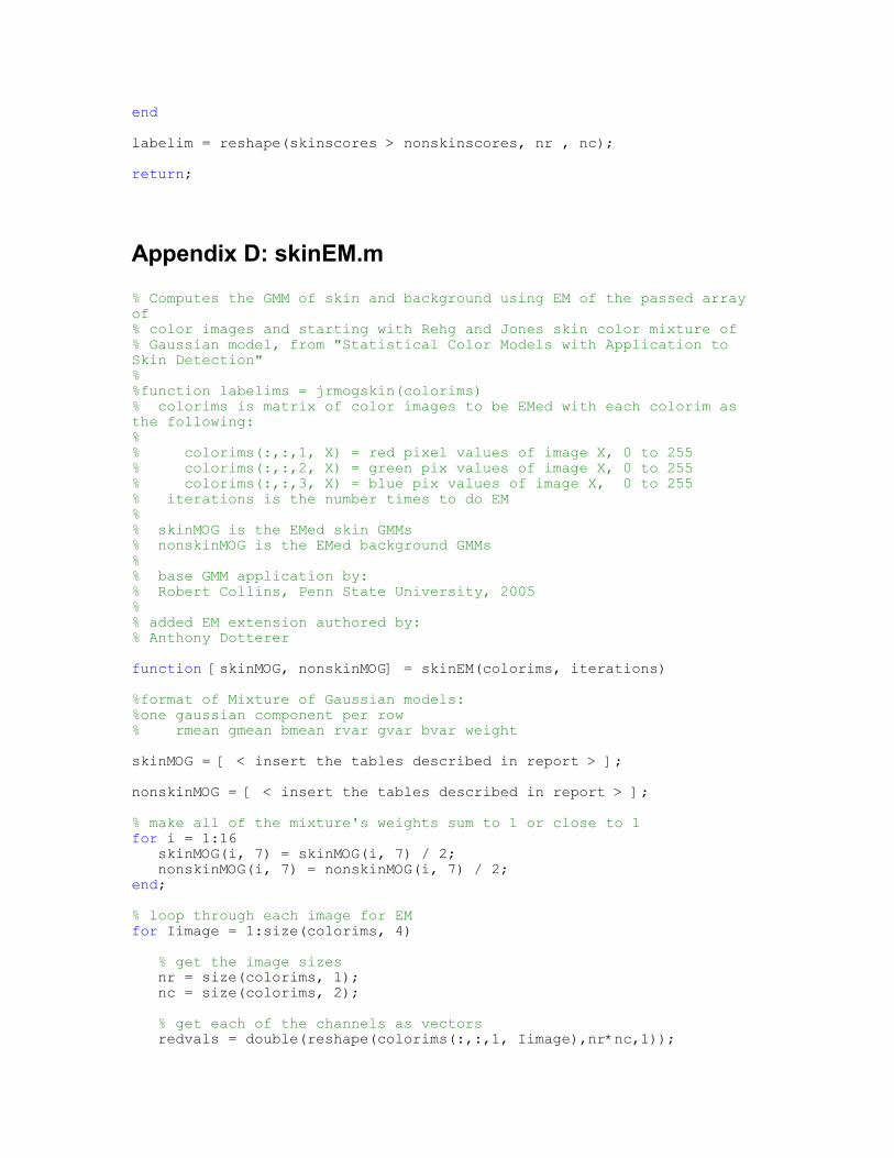
Appendix D: skinEM.m

% Computes the GMM of skin and background using EM of the passed array of% color images and starting with Rehg and Jones skin color mixture of% Gaussian model, from "Statistical Color Models with Application to Skin Detection"% %function labelims = jrmogskin(colorims)% colorims is matrix of color images to be EMed with each colorim as the following:% % colorims(:,:,1, X) = red pixel values of image X, 0 to 255% colorims(:,:,2, X) = green pix values of image X, 0 to 255% colorims(:,:,3, X) = blue pix values of image X, 0 to 255% iterations is the number times to do EM%% skinMOG is the EMed skin GMMs% nonskinMOG is the EMed background GMMs%% base GMM application by:% Robert Collins, Penn State University, 2005%% added EM extension authored by:% Anthony Dottererfunction [skinMOG, nonskinMOG] = skinEM(colorims, iterations)%format of Mixture of Gaussian models:%one gaussian component per row% rmean gmean bmean rvar gvar bvar weightskinMOG = [ < insert the tables described in report > ];nonskinMOG = [ < insert the tables described in report > ];% make all of the mixture's weights sum to 1 or close to 1 for i = 1:16 skinMOG(i, 7) = skinMOG(i, 7) / 2; nonskinMOG(i, 7) = nonskinMOG(i, 7) / 2;end;% loop through each image for EMfor Iimage = 1:size(colorims, 4) % get the image sizes nr = size(colorims, 1); nc = size(colorims, 2); % get each of the channels as vectors redvals = double(reshape(colorims(:,:,1, Iimage),nr*nc,1));

grevals = double(reshape(colorims(:,:,2, Iimage),nr*nc,1)); bluvals = double(reshape(colorims(:,:,3, Iimage),nr*nc,1)); % Construct a parameter vector that will hold each EM iteration lamda = zeros(32, 7, 1); lamda(1:16, :, 1) = skinMOG(:, :); lamda(17:32, :, 1) = nonskinMOG(: ,:); % let it iterate for a bit (just to see if this works at all) for t = 1:iterations % compute the propabilities of all datapoints for each class props = zeros(32, nr*nc); for i = 1:32 tmp = (redvals - lamda(i, 1, t)).^2 / lamda(i, 4, t) + (grevals - lamda(i, 2, t)).^2 / lamda(i, 5, t) + (bluvals - lamda(i, 3, t)).^2 / lamda(i, 6, t); tmp = lamda(i, 7, t) * exp(- tmp / 2) / ((2 * pi)^(3/2) * sqrt(lamda(i, 4, t)*lamda(i, 5, t)*lamda(i, 6, t))); props(i, :) = tmp(:, 1)'; end; % compute the sum of the propabilities of all datapoints for each class propssum = sum(props, 1); % compute expected classes for all datapoints for each class Estep = zeros(32, nr*nc); for i = 1:32 Estep(i, :) = props(i, :) ./ propssum; end; % compute the sum of the expected classes for all datapoints Estepsum = sum(Estep, 2); % compute the new weights for each class newWeights = []; for i = 1:32 newWeights(i) = Estepsum(i) / (nr*nc); end; % compute the new means for each class for each color newMeans = zeros(32, 3); for i = 1:32 if (Estepsum(i) ~= 0) tmp = sum(Estep(i, :)' .* redvals); newMeans(i, 1) = sum(Estep(i, :)' .* redvals) / Estepsum(i); newMeans(i, 2) = sum(Estep(i, :)' .* grevals) / Estepsum(i); newMeans(i, 3) = sum(Estep(i, :)' .* bluvals) / Estepsum(i); else newMeans(i, :) = lamda(i, 1:3, t); % 0 estep sum means 0 weight just pass previous value end; end; % compute the new variances for each class for each color % NOTE: if the variance drop to zero, because it is too small then use the smallest double value possible

newVar = zeros(32, 3); for i = 1:32 if (Estepsum(i) ~= 0) newVar(i, 1) = max(sum(Estep(i, :)' .* (redvals - newMeans(i, 1)).^2) / Estepsum(i), eps); newVar(i, 2) = max(sum(Estep(i, :)' .* (grevals - newMeans(i, 2)).^2) / Estepsum(i), eps); newVar(i, 3) = max(sum(Estep(i, :)' .* (bluvals - newMeans(i, 3)).^2) / Estepsum(i), eps); else newVar(i, :) = lamda(i, 4:6, t); % 0 estep sum means 0 weight just pass previous value end; end; % setup the next run in the lamda vector newLamda = zeros(32, 7, 1); for i = 1:32 newLamda(i, 1, 1) = newMeans(i, 1); newLamda(i, 2, 1) = newMeans(i, 2); newLamda(i, 3, 1) = newMeans(i, 3); newLamda(i, 4, 1) = newVar(i, 1); newLamda(i, 5, 1) = newVar(i, 2); newLamda(i, 6, 1) = newVar(i, 3); newLamda(i, 7, 1) = newWeights(i); end; lamda(:, :, t+1) = newLamda; %lamda(:, :, t+1) = [ newMeans, newVar, newWeights' ]; end; % replace the values of the skin and non-skin models skinMOG = lamda(1:16, :, t+1); nonskinMOG = lamda(17:32, :, t+1); end; % image loop% try to normalize the skin's total probalities to 1 and background's to 1totalSkinProp = sum(skinMOG(:, 7));totalNonskinProp = sum(nonskinMOG(:, 7));for i = 1:16 skinMOG(i, 7) = skinMOG(i, 7) / totalSkinProp; nonskinMOG(i, 7) = nonskinMOG(i, 7) / totalNonskinProp;end;return;

Appendix D: skinEM2.m

% Computes the GMM of skin and background using EM of the passed array of% color images and starting with Rehg and Jones skin color mixture of% Gaussian model, from "Statistical Color Models with Application to Skin Detection"%

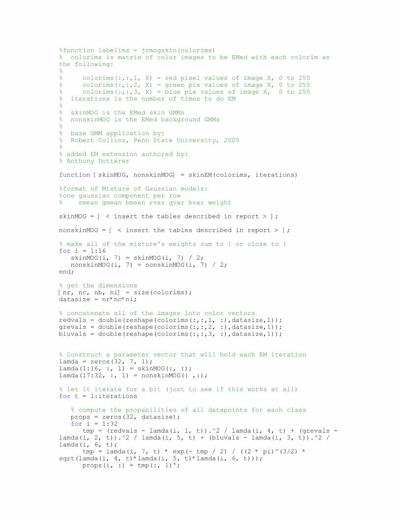
%function labelims = jrmogskin(colorims)% colorims is matrix of color images to be EMed with each colorim as the following:% % colorims(:,:,1, X) = red pixel values of image X, 0 to 255% colorims(:,:,2, X) = green pix values of image X, 0 to 255% colorims(:,:,3, X) = blue pix values of image X, 0 to 255% iterations is the number of times to do EM %% skinMOG is the EMed skin GMMs% nonskinMOG is the EMed background GMMs%% base GMM application by:% Robert Collins, Penn State University, 2005%% added EM extension authored by:% Anthony Dottererfunction [skinMOG, nonskinMOG] = skinEM(colorims, iterations)%format of Mixture of Gaussian models:%one gaussian component per row% rmean gmean bmean rvar gvar bvar weightskinMOG = [ < insert the tables described in report > ];nonskinMOG = [ < insert the tables described in report > ];% make all of the mixture's weights sum to 1 or close to 1 for i = 1:16 skinMOG(i, 7) = skinMOG(i, 7) / 2; nonskinMOG(i, 7) = nonskinMOG(i, 7) / 2;end;% get the dimensions[nr, nc, nb, ni] = size(colorims);datasize = nr*nc*ni;% concatenate all of the images into color vectors redvals = double(reshape(colorims(:,:,1, :),datasize,1));grevals = double(reshape(colorims(:,:,2, :),datasize,1));bluvals = double(reshape(colorims(:,:,3, :),datasize,1));

% Construct a parameter vector that will hold each EM iterationlamda = zeros(32, 7, 1);lamda(1:16, :, 1) = skinMOG(:, :);lamda(17:32, :, 1) = nonskinMOG(: ,:);% let it iterate for a bit (just to see if this works at all)for t = 1:iterations % compute the propabilities of all datapoints for each class props = zeros(32, datasize); for i = 1:32 tmp = (redvals - lamda(i, 1, t)).^2 / lamda(i, 4, t) + (grevals - lamda(i, 2, t)).^2 / lamda(i, 5, t) + (bluvals - lamda(i, 3, t)).^2 / lamda(i, 6, t); tmp = lamda(i, 7, t) * exp(- tmp / 2) / ((2 * pi)^(3/2) * sqrt(lamda(i, 4, t)*lamda(i, 5, t)*lamda(i, 6, t))); props(i, :) = tmp(:, 1)';

end; % compute the sum of the propabilities of all datapoints for each class propssum = sum(props, 1); % compute expected classes for all datapoints for each class Estep = zeros(32, datasize); for i = 1:32 Estep(i, :) = props(i, :) ./ propssum; end; % compute the sum of the expected classes for all datapoints Estepsum = sum(Estep, 2); % compute the new weights for each class newWeights = []; for i = 1:32 newWeights(i) = Estepsum(i) / datasize; end; % compute the new means for each class for each color newMeans = zeros(32, 3); for i = 1:32 if (Estepsum(i) ~= 0) tmp = sum(Estep(i, :)' .* redvals); newMeans(i, 1) = sum(Estep(i, :)' .* redvals) / Estepsum(i); newMeans(i, 2) = sum(Estep(i, :)' .* grevals) / Estepsum(i); newMeans(i, 3) = sum(Estep(i, :)' .* bluvals) / Estepsum(i); else newMeans(i, :) = lamda(i, 1:3, t); % 0 estep sum means 0 weight just pass previous value end; end; % compute the new variances for each class for each color % NOTE: if the variance drop to zero, because it is too small then use the smallest double value possible newVar = zeros(32, 3); for i = 1:32 if (Estepsum(i) ~= 0) newVar(i, 1) = max(sum(Estep(i, :)' .* (redvals - newMeans(i, 1)).^2) / Estepsum(i), eps); newVar(i, 2) = max(sum(Estep(i, :)' .* (grevals - newMeans(i, 2)).^2) / Estepsum(i), eps); newVar(i, 3) = max(sum(Estep(i, :)' .* (bluvals - newMeans(i, 3)).^2) / Estepsum(i), eps); else newVar(i, :) = lamda(i, 4:6, t); % 0 estep sum means 0 weight just pass previous value end; end; % setup the next run in the lamda vector newLamda = zeros(32, 7, 1); for i = 1:32 newLamda(i, 1, 1) = newMeans(i, 1); newLamda(i, 2, 1) = newMeans(i, 2); newLamda(i, 3, 1) = newMeans(i, 3); newLamda(i, 4, 1) = newVar(i, 1); newLamda(i, 5, 1) = newVar(i, 2);

newLamda(i, 6, 1) = newVar(i, 3); newLamda(i, 7, 1) = newWeights(i); end; lamda(:, :, t+1) = newLamda; %lamda(:, :, t+1) = [ newMeans, newVar, newWeights' ]; end;% replace the values of the skin and non-skin modelsskinMOG = lamda(1:16, :, t+1);nonskinMOG = lamda(17:32, :, t+1);

% try to normalize the skin's total probalities to 1 and background's to 1totalSkinProp = sum(skinMOG(:, 7));totalNonskinProp = sum(nonskinMOG(:, 7));for i = 1:16 skinMOG(i, 7) = skinMOG(i, 7) / totalSkinProp; nonskinMOG(i, 7) = nonskinMOG(i, 7) / totalNonskinProp;end;return;