Statistical Approaches to Establishing Bioequivalence€¦ · Guidance for Industry Statistical...

Guidance for Industry

Statistical Approaches toEstablishing Bioequivalence

U.S. Department of Health and Human ServicesFood and Drug Administration

Center for Drug Evaluation and Research (CDER)January 2001

BP

Guidance for Industry

Statistical Approaches toEstablishing Bioequivalence

Additional copies are available from:

Office of Training and CommunicationsDivision of Communications Management

Drug Information Branch, HFD-2105600 Fishers Lane

Rockville MD 20857(Tel) 301-827-4573

(Internet) http://www.fda.gov/cder/guidance/index.htm

U.S. Department of Health and Human ServicesFood and Drug Administration

Center for Drug Evaluation and Research (CDER)January 2001

BP

Table of Contents

I. INTRODUCTION..................................................................................................................................................................1

II. BACKGROUND....................................................................................................................................................................1

A. GENERAL............................................................................................................................................................................. 1B. STATISTICAL ...................................................................................................................................................................... 2

III. STATISTICAL MODEL......................................................................................................................................................3

IV. STATISTICAL APPROACHES FOR BIOEQUIVALENCE.........................................................................................3

A. AVERAGE BIOEQUIVALENCE.............................................................................................................................................. 4B. POPULATION BIOEQUIVALENCE ......................................................................................................................................... 5C. INDIVIDUAL BIOEQUIVALENCE ........................................................................................................................................... 6

V. STUDY DESIGN....................................................................................................................................................................7

A. EXPERIMENTAL DESIGN..................................................................................................................................................... 7B. SAMPLE SIZE AND DROPOUTS ........................................................................................................................................... 8

VI. STATISTICAL ANALYSIS ................................................................................................................................................9

A. LOGARITHMIC TRANSFORMATION .................................................................................................................................... 9B. DATA ANALYSIS .............................................................................................................................................................. 10

VII. MISCELLANEOUS ISSUES ........................................................................................................................................13

A. STUDIES IN MULTIPLE GROUPS....................................................................................................................................... 13B. CARRYOVER EFFECTS...................................................................................................................................................... 13C. OUTLIER CONSIDERATIONS ............................................................................................................................................. 14D. DISCONTINUITY................................................................................................................................................................ 15

REFERENCES ................................................................................................................................................................................16

APPENDIX A..................................................................................................................................................................................21

APPENDIX B..................................................................................................................................................................................25

APPENDIX C..................................................................................................................................................................................28

APPENDIX D..................................................................................................................................................................................32

APPENDIX E..................................................................................................................................................................................34

APPENDIX F..................................................................................................................................................................................35

APPENDIX G..................................................................................................................................................................................40

APPENDIX H..................................................................................................................................................................................45

J:\!GUIDANC\3616fnl.doc01/31/01

GUIDANCE FOR INDUSTRY1

Statistical Approachesto Establishing Bioequivalence

I. INTRODUCTION

This guidance provides recommendations to sponsors and applicants who intend, either before or afterapproval, to use equivalence criteria in analyzing in vivo or in vitro bioequivalence (BE) studies forinvestigational new drug applications (INDs), new drug applications (NDAs), abbreviated new drugapplications (ANDAs) and supplements to these applications. This guidance discusses threeapproaches for BE comparisons: average, population, and individual. The guidance focuses on how touse each approach once a specific approach has been chosen. This guidance replaces a prior FDAguidance entitled Statistical Procedures for Bioequivalence Studies Using a Standard Two-Treatment Crossover Design, which was issued in July 1992.

II. BACKGROUND

A. General

Requirements for submitting bioavailability (BA) and BE data in NDAs, ANDAs, andsupplements, the definitions of BA and BE, and the types of in vivo studies that are appropriateto measure BA and establish BE are set forth in 21 CFR part 320. This guidance providesrecommendations on how to meet provisions of part 320 for all drug products.

Defined as relative BA, BE involves comparison between a test (T) and reference (R) drugproduct, where T and R can vary, depending on the comparison to be performed (e.g., to-be-marketed dosage form versus clinical trial material, generic drug versus reference listed drug,

1 This guidance has been prepared by the Population and Individual Bioequivalence Working Group of the

Biopharmaceutics Coordinating Committee in the Office of Pharmaceutical Science, Center for Drug Evaluation andResearch (CDER) at the Food and Drug Administration (FDA).

This guidance represents the Food and Drug Administration's current thinking on this topic. Itdoes not create or confer any rights for or on any person and does not operate to bind FDA or thepublic. An alternative approach may be used if such approach satisfies the requirements of theapplicable statutes and regulations.

2

drug product changed after approval versus drug product before the change). Although BAand BE are closely related, BE comparisons normally rely on (1) a criterion, (2) a confidenceinterval for the criterion, and (3) a predetermined BE limit. BE comparisons could also be usedin certain pharmaceutical product line extensions, such as additional strengths, new dosageforms (e.g., changes from immediate release to extended release), and new routes ofadministration. In these settings, the approaches described in this guidance can be used todetermine BE. The general approaches discussed in this guidance may also be useful whenassessing pharmaceutical equivalence or performing equivalence comparisons in clinicalpharmacology studies and other areas.

B. Statistical

In the July 1992 guidance on Statistical Procedures for Bioequivalence Studies Using aStandard Two-Treatment Crossover Design (the 1992 guidance), CDER recommended thata standard in vivo BE study design be based on the administration of either single or multipledoses of the T and R products to healthy subjects on separate occasions, with randomassignment to the two possible sequences of drug product administration. The 1992 guidancefurther recommended that statistical analysis for pharmacokinetic measures, such as area underthe curve (AUC) and peak concentration (Cmax), be based on the two one-sided testsprocedure to determine whether the average values for the pharmacokinetic measuresdetermined after administration of the T and R products were comparable. This approach istermed average bioequivalence and involves the calculation of a 90% confidence interval forthe ratio of the averages (population geometric means) of the measures for the T and Rproducts. To establish BE, the calculated confidence interval should fall within a BE limit,usually 80-125% for the ratio of the product averages.2 In addition to this general approach,the 1992 guidance provided specific recommendations for (1) logarithmic transformation ofpharmacokinetic data, (2) methods to evaluate sequence effects, and (3) methods to evaluateoutlier data.

Although average BE is recommended for a comparison of BA measures in most BE studies,this guidance describes two new approaches, termed population and individualbioequivalence. These new approaches may be useful, in some instances, for analyzingin vitro and in vivo BE studies.3 The average BE approach focuses only on the comparison ofpopulation averages of a BE measure of interest and not on the variances of the measure for the

2 For a broad range of drugs, a BE limit of 80 to 125% for the ratio of the product averages has been adopted

for use of an average BE criterion. Generally, the BE limit of 80 to 125% is based on a clinical judgment that a testproduct with BA measures outside this range should be denied market access.

3 For additional recommendations on in vivo studies, see the FDA guidance for industry on Bioavailabilityand Bioequivalence Studies for Orally Administered Drug Products C General Considerations. Additionalrecommendations on in vitro studies will be provided in an FDA guidance for industry on Bioavailability andBioequivalence Studies for Nasal Aerosols and Nasal Sprays for Local Action, when finalized.

3

T and R products. The average BE method does not assess a subject-by-formulationinteraction variance, that is, the variation in the average T and R difference among individuals. In contrast, population and individual BE approaches include comparisons of both averages andvariances of the measure. The population BE approach assesses total variability of the measurein the population. The individual BE approach assesses within-subject variability for the T andR products, as well as the subject-by-formulation interaction.

III. STATISTICAL MODEL

Statistical analyses of BE data are typically based on a statistical model for the logarithm of the BAmeasures (e.g., AUC and Cmax). The model is a mixed-effects or two-stage linear model. Eachsubject, j, theoretically provides a mean for the log-transformed BA measure for each formulation, µTj

and µRj for the T and R formulations, respectively. The model assumes that these subject-specificmeans come from a distribution with population means µT and µR, and between-subject variances σBT

2

and σBR2, respectively. The model allows for a correlation, ρ, between µTj and µRj. The subject-by-

formulation interaction variance component (Schall and Luus 1993), σD2, is related to these parameters

as follows:

σD2 = variance of (µTj - µRj)

= (σBT - σBR)2 + 2 (1-ρ)σBTσBR Equation 1

For a given subject, the observed data for the log-transformed BA measure are assumed to beindependent observations from distributions with means µTj and µRj, and within-subject variances σWT

2

and σWR2. The total variances for each formulation are defined as the sum of the within- and between-

subject components (i.e., σTT2 = σWT

2 + σBT2 and σTR

2 = σWR2 + σBR

2). For analysis of crossoverstudies, the means are given additional structure by the inclusion of period and sequence effect terms.

IV. STATISTICAL APPROACHES FOR BIOEQUIVALENCE

The general structure of a BE criterion is that a function (Θ) of population measures should bedemonstrated to be no greater than a specified value (θ). Using the terminology of statistical hypothesistesting, this is accomplished by testing the hypothesis H0: Θ>θ versus HA: Θ#θ at a desired level ofsignificance, often 5%. Rejection of the null hypothesis H0 (i.e., demonstrating that the estimate of Θ isstatistically significantly less than θ) results in a conclusion of BE. The choice of Θ and θ differs inaverage, population, and individual BE approaches.

A general objective in assessing BE is to compare the log-transformed BA measure after administrationof the T and R products. As detailed in Appendix A, population and individual approaches are basedon the comparison of an expected squared distance between the T and R formulations to the expected

4

squared distance between two administrations of the R formulation. An acceptable T formulation is onewhere the T-R distance is not substantially greater than the R-R distance. In both population andindividual BE approaches, this comparison appears as a comparison to the reference variance, which isreferred to as scaling to the reference variability.

Population and individual BE approaches, but not the average BE approach, allow two types of scaling: reference-scaling and constant-scaling. Reference-scaling means that the criterion used is scaled to thevariability of the R product, which effectively widens the BE limit for more variable reference products. Although generally sufficient, use of reference-scaling alone could unnecessarily narrow the BE limit fordrugs and/or drug products that have low variability but a wide therapeutic range. This guidance,therefore, recommends mixed-scaling for the population and individual BE approaches (section IV.Band C). With mixed scaling, the reference-scaled form of the criterion should be used if the referenceproduct is highly variable; otherwise, the constant-scaled form should be used.

A. Average Bioequivalence

The following criterion is recommended for average BE:

(µT - µR)2 # θA2 Equation 2

where

µT = population average response of the log-transformed measure for the T formulation µR = population average response of the log-transformed measure for the R formulation

as defined in section III above.

5

This criterion is equivalent to:

-θA # (µT - µR) # θA Equation 3

and, usually, θA = ln(1.25).

B. Population Bioequivalence

The following mixed-scaling approach is recommended for population BE (i.e., use thereference-scaled method if the estimate of σTR > σT0 and the constant-scaled method if theestimate of σTR # σT0).

The recommended criteria are:

! Reference-Scaled:

(µT - µR)2 + (σTT2 - σTR

2)-------------------------------- # θp Equation 4

σTR2

or

! Constant-Scaled:

(µT - µR)2 + (σTT2 - σTR

2)-------------------------------- # θp Equation 5 σT0

2

where:

µT = population average response of the log-transformed measure for the T formulation

µR = population average response of the log-transformed measure for the R formulation

σTT2 = total variance (i.e., sum of within- and between-subject

variances) of the T formulationσTR

2 = total variance (i.e., sum of within- and between-subject variances) of the R formulation

σT02 = specified constant total variance

θp = BE limit

6

Equations 4 and 5 represent an aggregate approach where a single criterion on the left-handside of the equation encompasses two major components: (1) the difference between the T andR population averages (µT - µR), and (2) the difference between the T and R total variances(σTT

2 - σTR2). This aggregate measure is scaled to the total variance of the R product or to a

constant value (σT02, a standard that relates to a limit for the total variance), whichever is

greater.

The specification of both σT0 and θP relies on the establishment of standards. The generation ofthese standards is discussed in Appendix A. When the population BE approach is used, inaddition to meeting the BE limit based on confidence bounds, the point estimate of thegeometric test/reference mean should fall within 80-125%.

C. Individual Bioequivalence

The following mixed-scaling approach is one approach for individual BE (i.e., use the reference-scaled method if the estimate of σWR > σW0, and the constant-scaled method if the estimate ofσWR # σW0). Also see section VII.D, Discontinuity, for further discussion.

The recommended criteria are:

! Reference-Scaled:

(µT - µR)2 + σD2 + (σWT

2 - σWR2)

----------------------------------------- # θI Equation 6 σWR

2

or

! Constant-Scaled:

(µT - µR)2 + σD2 + (σWT

2 - σWR2)

----------------------------------------- # θI Equation 7 σW0

2

where:

µT = population average response of the log-transformed measure for the T formulation

µR = population average response of the log-transformed measure for the R formulation

σD2 = subject-by-formulation interaction variance component

7

σWT2 = within-subject variance of the T formulation

σWR2 = within-subject variance of the R formulation

σW02 = specified constant within-subject variance

θI = BE limit

Equations 6 and 7 represent an aggregate approach where a single criterion on the left-handside of the equation encompasses three major components: (1) the difference between the Tand R population averages (µT - µR), (2) subject-by-formulation interaction (σD

2), and (3) thedifference between the T and R within-subject variances (σWT

2 - σWR2). This aggregate

measure is scaled to the within-subject variance of the R product or to a constant value (σW02, a

standard that relates to a limit for the within-subject variance), whichever is greater.

The specification of both σW0 and θI relies on the establishment of standards. The generation ofthese standards is discussed in Appendix A. When the individual BE approach is used, inaddition to meeting the BE limit based on confidence bounds, the point estimate of thegeometric test/reference mean ratio should fall within 80-125%.

V. STUDY DESIGN

A. Experimental Design

1. Nonreplicated Designs

A conventional nonreplicated design, such as the standard two-formulation, two-period,two-sequence crossover design, can be used to generate data where an average orpopulation approach is chosen for BE comparisons. Under certain circumstances,parallel designs can also be used.

2. Replicated Crossover Designs

Replicated crossover designs can be used irrespective of which approach is selected toestablish BE, although they are not necessary when an average or population approachis used. Replicated crossover designs are critical when an individual BE approach isused to allow estimation of within-subject variances for the T and R measures and thesubject-by-formulation interaction variance component. The following four-period,two-sequence, two-formulation design is recommended for replicated BE studies (seeAppendix B for further discussion of replicated crossover designs).

8

Period

1 2 3 4

1 T R T RSequence

2 R T R T

For this design, the same lots of the T and R formulations should be used for thereplicated administration. Each period should be separated by an adequate washoutperiod.

Other replicated crossover designs are possible. For example, a three-period design,as shown below, could be used.

Period

1 2 3

1 T R TSequence

2 R T R

A greater number of subjects would be encouraged for the three-period designcompared to the recommended four-period design to achieve the same statistical powerto conclude BE (see Appendix C).

B. Sample Size and Dropouts

A minimum number of 12 evaluable subjects should be included in any BE study. When anaverage BE approach is selected using either nonreplicated or replicated designs, methodsappropriate to the study design should be used to estimate sample sizes. The number ofsubjects for BE studies based on either the population or individual BE approach can beestimated by simulation if analytical approaches for estimation are not available. Furtherinformation on sample size is provided in Appendix C.

Sponsors should enter a sufficient number of subjects in the study to allow for dropouts. Because replacement of subjects during the study could complicate the statistical model andanalysis, dropouts generally should not be replaced. Sponsors who wish to replace dropoutsduring the study should indicate this intention in the protocol. The protocol should also state

9

whether samples from replacement subjects, if not used, will be assayed. If the dropout rate ishigh and sponsors wish to add more subjects, a modification of the statistical analysis may berecommended. Additional subjects should not be included after data analysis unless the trialwas designed from the beginning as a sequential or group sequential design.

VI. STATISTICAL ANALYSIS

The following sections provide recommendations on statistical methodology for assessment of average,population, and individual BE.

A. Logarithmic Transformation

1. General Procedures

This guidance recommends that BE measures (e.g., AUC and Cmax) be log-transformed using either common logarithms to the base 10 or natural logarithms (seeAppendix D). The choice of common or natural logs should be consistent and shouldbe stated in the study report. The limited sample size in a typical BE study precludes areliable determination of the distribution of the data set. Sponsors and/or applicants arenot encouraged to test for normality of error distribution after log-transformation, norshould they use normality of error distribution as a reason for carrying out the statisticalanalysis on the original scale. Justification should be provided if sponsors or applicantsbelieve that their BE study data should be statistically analyzed on the original ratherthan on the log scale.

2. Presentation of Data

The drug concentration in biological fluid determined at each sampling time point shouldbe furnished on the original scale for each subject participating in the study. Thepharmacokinetic measures of systemic exposure should also be furnished on the originalscale. The mean, standard deviation, and coefficient of variation for each variableshould be computed and tabulated in the final report.

In addition to the arithmetic mean and associated standard deviation (or coefficient ofvariation) for the T and R products, geometric means (antilog of the means of the logs)should be calculated for selected BE measures. To facilitate BE comparisons, themeasures for each individual should be displayed in parallel for the formulations tested. In particular, for each BE measure the ratio of the individual geometric mean of the Tproduct to the individual geometric mean of the R product should be tabulated side byside for each subject. The summary tables should indicate in which sequence each

10

subject received the product.

B. Data Analysis

1. Average Bioequivalence

a. Overview

Parametric (normal-theory) methods are recommended for the analysis of log-transformed BE measures. For average BE using the criterion stated inequations 2 or 3 (section III.A), the general approach is to construct a 90%confidence interval for the quantity µT-µR and to reach a conclusion of averageBE if this confidence interval is contained in the interval [-θA , θA]. Due to thenature of normal-theory confidence intervals, this is equivalent to carrying outtwo one-sided tests of hypothesis at the 5% level of significance (Schuirmann1987).

The 90% confidence interval for the difference in the means of the log-transformed data should be calculated using methods appropriate to theexperimental design. The antilogs of the confidence limits obtained constitutethe 90% confidence interval for the ratio of the geometric means between the Tand R products.

b. Nonreplicated Crossover Designs

For nonreplicated crossover designs, this guidance recommends parametric(normal-theory) procedures to analyze log-transformed BA measures. Generallinear model procedures available in PROC GLM in SAS or equivalentsoftware are preferred, although linear mixed-effects model procedures can alsobe indicated for analysis of nonreplicated crossover studies.

For example, for a conventional two-treatment, two-period, two-sequence (2 x2) randomized crossover design, the statistical model typically includes factorsaccounting for the following sources of variation: sequence, subjects nested insequences, period, and treatment. The Estimate statement in SAS PROCGLM, or equivalent statement in other software, should be used to obtainestimates for the adjusted differences between treatment means and thestandard error associated with these differences.

c. Replicated Crossover Designs

11

Linear mixed-effects model procedures, available in PROC MIXED in SAS orequivalent software, should be used for the analysis of replicated crossoverstudies for average BE. Appendix E includes an example of SAS programstatements.

d. Parallel Designs

For parallel designs, the confidence interval for the difference of means in thelog scale can be computed using the total between-subject variance. As in theanalysis for replicated designs (section VI. B.1.b), equal variances should notbe assumed.

2. Population Bioequivalence

a. Overview

Analysis of BE data using the population approach (section IV.B) should focusfirst on estimation of the mean difference between the T and R for the log-transformed BA measure and estimation of the total variance for each of thetwo formulations. This can be done using relatively simple unbiased estimatorssuch as the method of moments (MM) (Chinchilli 1996, and Chinchilli andEsinhart 1996). After the estimation of the mean difference and the varianceshas been completed, a 95% upper confidence bound for the population BEcriterion can be obtained, or equivalently a 95% upper confidence bound for alinearized form of the population BE criterion can be obtained. Population BEshould be considered to be established for a particular log-transformed BAmeasure if the 95% upper confidence bound for the criterion is less than orequal to the BE limit, θP, or equivalently if the 95% upper confidence bound forthe linearized criterion is less than or equal to 0.

To obtain the 95% upper confidence bound of the criterion, intervals based onvalidated approaches can be used. Validation approaches should be reviewedwith appropriate staff in CDER. Appendix F includes an example of upperconfidence bound determination using a population BE approach.

b. Nonreplicated Crossover Designs

For nonreplicated crossover studies, any available method (e.g., SAS PROCGLM or equivalent software) can be used to obtain an unbiased estimate of themean difference in log-transformed BA measures between the T and Rproducts. The total variance for each formulation should be estimated by the

12

usual sample variance, computed separately in each sequence and then pooledacross sequences.

c. Replicated Crossover Designs

For replicated crossover studies, the approach should be the same as fornonreplicated crossover designs, but care should be taken to obtain properestimates of the total variances. One approach is to estimate the within- andbetween-subject components separately, as for individual BE (see sectionVI.B.3), and then sum them to obtain the total variance. The method for theupper confidence bound should be consistent with the method used forestimating the variances.

d. Parallel Designs

The estimate of the means and variances from parallel designs should be thesame as for nonreplicated crossover designs. The method for the upperconfidence bound should be modified to reflect independent rather than pairedsamples and to allow for unequal variances.

3. Individual Bioequivalence

Analysis of BE data using an individual BE approach (section IV.C) should focus onestimation of the mean difference between T and R for the log-transformed BAmeasure, the subject-by-formulation interaction variance, and the within-subjectvariance for each of the two formulations. For this purpose, we recommend the MMapproach.

To obtain the 95% upper confidence bound of a linearized form of the individual BEcriterion, intervals based on validated approaches can be used. An example isdescribed in Appendix G. After the estimation of the mean difference and the varianceshas been completed, a 95% upper confidence bound for the individual BE criterion canbe obtained, or equivalently a 95% upper confidence bound for a linearized form of theindividual BE criterion can be obtained. Individual BE should be considered to beestablished for a particular log-transformed BA measure if the 95% upper confidencebound for the criterion is less than or equal to the BE limit, θI, or equivalently if the 95%upper confidence bound for the linearized criterion is less than or equal to 0.

The restricted maximum likelihood (REML) method may be useful to estimate meandifferences and variances when subjects with some missing data are included in thestatistical analysis. A key distinction between the REML and MM methods relates to

13

differences in estimating variance terms and is further discussed in Appendix H. Sponsors considering alternative methods to REML or MM are encouraged to discusstheir approaches with appropriate CDER review staff prior to submitting theirapplications.

VII. MISCELLANEOUS ISSUES

A. Studies in Multiple Groups

If a crossover study is carried out in two or more groups of subjects (e.g., if for logisticalreasons only a limited number of subjects can be studied at one time), the statistical modelshould be modified to reflect the multigroup nature of the study. In particular, the model shouldreflect the fact that the periods for the first group are different from the periods for the secondgroup. This applies to all of the approaches (average, population, and individual BE) describedin this guidance.

If the study is carried out in two or more groups and those groups are studied at different clinicalsites, or at the same site but greatly separated in time (months apart, for example), questionsmay arise as to whether the results from the several groups should be combined in a singleanalysis. Such cases should be discussed with the appropriate CDER review division.

A sequential design, in which the decision to study a second group of subjects is based on theresults from the first group, calls for different statistical methods and is outside the scope of thisguidance. Those wishing to use a sequential design should consult the appropriate CDERreview division.

B. Carryover Effects

Use of crossover designs for BE studies allows each subject to serve as his or her own controlto improve the precision of the comparison. One of the assumptions underlying this principle isthat carryover effects (also called residual effects) are either absent (the response to aformulation administered in a particular period of the design is unaffected by formulationsadministered in earlier periods) or equal for each formulation and preceding formulation. Ifcarryover effects are present in a crossover study and are not equal, the usual crossoverestimate of µT-µR could be biased. One limitation of a conventional two-formulation, two-period, two-sequence crossover design is that the only statistical test available for the presenceof unequal carryover effects is the sequence test in the analysis of variance (ANOVA) for thecrossover design. This is a between-subject test, which would be expected to have poordiscriminating power in a typical BE study. Furthermore, if the possibility of unequal carryovereffects cannot be ruled out, no unbiased estimate of µT-µR based on within-subject

14

comparisons can be obtained with this design.

For replicated crossover studies, a within-subject test for unequal carryover effects can beobtained under certain assumptions. Typically only first-order carryover effects are consideredof concern (i.e., the carryover effects, if they occur, only affect the response to the formulationadministered in the next period of the design). Under this assumption, consideration ofcarryover effects could be more complicated for replicated crossover studies than fornonreplicated studies. The carryover effect could depend not only on the formulation thatpreceded the current period, but also on the formulation that is administered in the currentperiod. This is called a direct-by-carryover interaction. The need to consider more than justsimple first-order carryover effects has been emphasized (Fleiss 1989). With a replicatedcrossover design, a within-subject estimate of µT-µR unbiased by general first-order carryovereffects can be obtained, but such an estimate could be imprecise, reducing the power of thestudy to conclude BE.

In most cases, for both replicated and nonreplicated crossover designs, the possibility ofunequal carryover effects is considered unlikely in a BE study under the following circumstances:

! It is a single-dose study.

! The drug is not an endogenous entity.

! More than an adequate washout period has been allowed between periods of the studyand in the subsequent periods the predose biological matrix samples do not exhibit adetectable drug level in any of the subjects.

! The study meets all scientific criteria (e.g., it is based on an acceptable study protocoland it contains sufficient validated assay methodology).

The possibility of unequal carryover effects can also be discounted for multiple-dose studiesand/or studies in patients, provided that the drug is not an endogenous entity and the studiesmeet all scientific criteria as described above. Under all other circumstances, the sponsor orapplicant could be asked to consider the possibility of unequal carryover effects, including adirect-by-carryover interaction. If there is evidence of carryover effects, sponsors shoulddescribe their proposed approach in the study protocol, including statistical tests for thepresence of such effects and procedures to be followed. Sponsors who suspect that carryovereffects might be an issue may wish to conduct a BE study with parallel designs.

C. Outlier Considerations

Outlier data in BE studies are defined as subject data for one or more BA measures that are

15

discordant with corresponding data for that subject and/or for the rest of the subjects in a study. Because BE studies are usually carried out as crossover studies, the most important type ofsubject outlier is the within-subject outlier, where one subject or a few subjects differ notablyfrom the rest of the subjects with respect to a within-subject T-R comparison. The existence ofa subject outlier with no protocol violations could indicate one of the following situations:

1. Product Failure

Product failure could occur, for example, when a subject exhibits an unusually high orlow response to one or the other of the products because of a problem with the specificdosage unit administered. This could occur, for example, with a sustained and/ordelayed-release dosage form exhibiting dose dumping or a dosage unit with a coatingthat inhibits dissolution.

2. Subject-by-Formulation Interaction

A subject-by-formulation interaction could occur when an individual is representative ofsubjects present in the general population in low numbers, for whom the relative BA ofthe two products is markedly different than for the majority of the population, and forwhom the two products are not bioequivalent, even though they might be bioequivalentin the majority of the population.

In the case of product failure, the unusual response could be present for either the T or Rproduct. However, in the case of a subpopulation, even if the unusual response is observed onthe R product, there could still be concern for lack of interchangeability of the two products. For these reasons, deletion of outlier values is generally discouraged, particularly fornonreplicated designs. With replicated crossover designs, the retest character of these designsshould indicate whether to delete an outlier value or not. Sponsors or applicants with thesetypes of data sets may wish to review how to handle outliers with appropriate review staff.

D. Discontinuity

The mixed-scaling approach has a discontinuity at the changeover point, σW0 (individual BEcriterion) or σT0 (population BE criterion), from constant- to reference-scaling. For example, ifthe estimate of the within-subject standard deviation of the reference is just above thechangeover point, the confidence interval will be wider than just below. In this context, theconfidence interval could pass the predetermined BE limit if the estimate is just below theboundary and could fail if just above. This guidance recommends that sponsors applying theindividual BE approach may use either reference-scaling or constant-scaling at either side of thechangeover point. With this approach, the multiple testing inflates the type I error rate slightly,to approximately 6.5%, but only over a small interval of σWR (about 0.18-0.20).

16

REFERENCES

Anderson, S., and W.W. Hauck, 1990, "Consideration of Individual Bioequivalence," J.Pharmacokin. Biopharm., 18:259-73.

Anderson, S., 1993, "Individual Bioequivalence: A Problem of Switchability (with discussion),"Biopharmaceutical Reports, 2(2):1-11.

Anderson, S., 1995, "Current Issues of Individual Bioequivalence," Drug Inf. J., 29:961-4.

Chen, M.-L., 1997, "Individual Bioequivalence — A Regulatory Update (with discussion)," J.Biopharm. Stat., 7:5-111.

Chen, M.-L., R. Patnaik, W.W. Hauck, D.J. Schuirmann, T. Hyslop, R.L. Williams, and the FDAPopulation and Individual Bioequivalence Working Group, 2000, AAn Individual BioequivalenceCriterion: Regulatory Considerations,@ Stat. Med., 19:2821-42.

Chen, M.-L., S.-C. Lee, M.-J. Ng, D.J. Schuirmann, L. J. Lesko, and R.L. Williams, 2000,"Pharmacokinetic analysis of bioequivalence trials: Implications for sex-related issues in clinicalpharmacology and biopharmaceutics," Clin. Pharmacol. Ther., 68(5):510-21.

Chinchilli, V.M., 1996, "The Assessment of Individual and Population Bioequivalence," J. Biopharm.Stat., 6:1-14.

Chinchilli, V.M., and J.D. Esinhart, 1996, ADesign and Analysis of Intra-Subject Variability in Cross-Over Experiments,@ Stat. Med., 15:1619-34.

Chow, S.-C., 1999, AIndividual Bioequivalence — A Review of the FDA Draft Guidance,@ Drug Inf.J., 33:435-44.

Diletti E., D. Hauschke, and V.W. Steinijans, 1991, ASample Size Determination for BioequivalenceAssessment By Means of Confidence Intervals,@ Int. J. Clin. Pharmacol. Therap., 29:1-8.

Efron, B., 1987, "Better Bootstrap Confidence Intervals (with discussion)," J. Amer. Stat. Assoc.,82:171-201.

Efron, B., and R.J. Tibshirani, 1993, An Introduction to the Bootstrap, Chapman and Hall, Ch. 14.

17

Ekbohm, G., and H. Melander, 1989, "The Subject-by-Formulation Interaction as a Criterion forInterchangeability of Drugs," Biometrics, 45:1249-54.

Ekbohm, G., and H. Melander, 1990, "On Variation, Bioequivalence and Interchangeability," Report14, Department of Statistics, Swedish University of Agricultural Sciences.

Endrenyi, L., and M. Schulz, 1993, "Individual Variation and the Acceptance of AverageBioequivalence," Drug Inf. J., 27:195-201.

Endrenyi, L., 1993, "A Procedure for the Assessment of Individual Bioequivalence," in Bio-International: Bioavailability, Bioequivalence and Pharmacokinetics (H.H.Blume, K.K. Midha,eds.), Medpharm Publications, 141-6.

Endrenyi, L., 1994, "A Method for the Evaluation of Individual Bioequivalence," Int. J. Clin.Pharmacol. Therap., 32:497-508.

Endrenyi, L., 1995, "A Simple Approach for the Evaluation of Individual Bioequivalence," Drug Inf. J.,29:847-55.

Endrenyi, L., and K.K. Midha, 1998, AIndividual Bioequivalence — Has Its Time Come?,@ Eur. J.Pharm. Sci., 6:271-8.

Endrenyi, L., G.L. Amidon, K.K. Midha, and J.P. Skelly, 1998, AIndividual Bioequivalence: Attractivein Principle, Difficult in Practice,@ Pharm. Res., 15:1321-5.

Endrenyi, L., and Y. Hao, 1998, AAsymmetry of the Mean-Variability Tradeoff Raises QuestionsAbout the Model in Investigations of Individual Bioequivalence,@ Int. J. Pharmacol. Therap., 36:450-7.

Endrenyi, L., and L. Tothfalusi, 1999, ASubject-by-Formulation Interaction in Determination ofIndividual Bioequivalence: Bias and Prevalence,@ Pharm. Res., 16:186-8.

Esinhart, J.D., and V.M. Chinchilli, 1994, "Sample Size Considerations for Assessing IndividualBioequivalence Based on the Method of Tolerance Interval," Int. J. Clin. Pharmacol. Therap.,32(1):26-32.

Esinhart, J.D., and V.M. Chinchilli, 1994, "Extension to the Use of Tolerance Intervals for theAssessment of Individual Bioequivalence," J. Biopharm. Stat., 4(1):39-52.

Fleiss, J.L., 1989, AA Critique of Recent Research on the Two-Treatment Crossover Design,@Controlled Clinical Trials, 10:237-43.

18

Graybill, F., and C.M. Wang, 1980, AConfidence Intervals on Nonnegative Linear Combinations ofVariances,@ J. Amer. Stat. Assoc., 75:869-73.

Hauck, W.W., and S. Anderson, 1984, "A New Statistical Procedure for Testing Equivalence in Two-Group Comparative Bioavailability Trials," J. Pharmacokin. Biopharm., 12:83-91.

Hauck, W.W., and S. Anderson, 1992, "Types of Bioequivalence and Related StatisticalConsiderations," Int. J. Clin. Pharmacol. Therap., 30:181-7.

Hauck, W.W., and S. Anderson, 1994, "Measuring Switchability and Prescribability: When is AverageBioequivalence Sufficient?," J. Pharmacokin. Biopharm., 22:551-64.

Hauck, W.W., M.-L. Chen, T. Hyslop, R. Patnaik, D. Schuirmann, and R.L. Williams for the FDAPopulation and Individual Bioequivalence Working Group, 1996, AMean Difference vs. VariabilityReduction: Tradeoffs in Aggregate Measures for Individual Bioequivalence," Int. J. Clin. Pharmacol.Therap., 34:535-41.

Holder, D.J., and F. Hsuan, 1993, "Moment-Based Criteria for Determining Bioequivalence,"Biometrika, 80:835-46.

Holder, D.J., and F. Hsuan, 1995, "A Moment-Based Method for Determining IndividualBioequivalence," Drug Inf. J., 29:965-79.

Howe, W.G., 1974. AApproximate Confidence Limits on the Mean of X+Y Where X and Y are TwoTabled Independent Random Variables,@ J. Amer. Stat. Assoc., 69:789-94.

Hsu, J.C., J.T.G. Hwang, H.-K. Liu, and S.J. Ruberg, 1994, AConfidence Intervals Associated withTests for Bioequivalence,@ Biometrika, 81:103-14.

Hwang, S., P.B. Huber, M. Hesney, and K.C. Kwan, 1978, "Bioequivalence and Interchangeability,"J. Pharm. Sci., 67:IV "Open Forum."

Hyslop, T., F. Hsuan, and D.J. Holder, 2000, AA Small-Sample Confidence Interval Approach toAssess Individual Bioequivalence,@ Stat. Med., 19:2885-97.

Kimanani, E.K., and D. Potvin, 1998, AParametric Confidence Interval for a Moment-Based ScaledCriterion for Individual Bioequivalence,@ J. Pharm. Biopharm., 25:595-614.

Liu, J.-P, 1995, AUse of the Repeated Crossover Designs in Assessing Bioequivalence,@ Stat. Med.,14:1067-78.

19

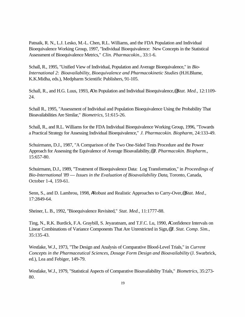
Patnaik, R. N., L.J. Lesko, M.-L. Chen, R.L. Williams, and the FDA Population and IndividualBioequivalence Working Group, 1997, "Individual Bioequivalence: New Concepts in the StatisticalAssessment of Bioequivalence Metrics," Clin. Pharmacokin., 33:1-6.

Schall, R., 1995, "Unified View of Individual, Population and Average Bioequivalence," in Bio-International 2: Bioavailability, Bioequivalence and Pharmacokinetic Studies (H.H.Blume,K.K.Midha, eds.), Medpharm Scientific Publishers, 91-105.

Schall, R., and H.G. Luus, 1993, AOn Population and Individual Bioequivalence,@ Stat. Med., 12:1109-24.

Schall R., 1995, "Assessment of Individual and Population Bioequivalence Using the Probability ThatBioavailabilities Are Similar," Biometrics, 51:615-26.

Schall, R., and R.L. Williams for the FDA Individual Bioequivalence Working Group, 1996, "Towardsa Practical Strategy for Assessing Individual Bioequivalence," J. Pharmacokin. Biopharm, 24:133-49.

Schuirmann, D.J., 1987, "A Comparison of the Two One-Sided Tests Procedure and the PowerApproach for Assessing the Equivalence of Average Bioavailability,@ J. Pharmacokin. Biopharm.,15:657-80.

Schuirmann, D.J., 1989, "Treatment of Bioequivalence Data: Log Transformation," in Proceedings ofBio-International '89 — Issues in the Evaluation of Bioavailability Data, Toronto, Canada,October 1-4, 159-61.

Senn, S., and D. Lambrou, 1998, ARobust and Realistic Approaches to Carry-Over,@ Stat. Med.,17:2849-64.

Sheiner, L. B., 1992, "Bioequivalence Revisited," Stat. Med., 11:1777-88.

Ting, N., R.K. Burdick, F.A. Graybill, S. Jeyaratnam, and T.F.C. Lu, 1990, AConfidence Intervals onLinear Combinations of Variance Components That Are Unrestricted in Sign,@ J. Stat. Comp. Sim.,35:135-43.

Westlake, W.J., 1973, "The Design and Analysis of Comparative Blood-Level Trials," in CurrentConcepts in the Pharmaceutical Sciences, Dosage Form Design and Bioavailability (J. Swarbrick,ed.), Lea and Febiger, 149-79.

Westlake, W.J., 1979, "Statistical Aspects of Comparative Bioavailability Trials," Biometrics, 35:273-80.

20

Westlake, W.J., 1981, "Response to Kirkwood, TBL.: Bioequivalence Testing — A Need toRethink," Biometrics, 37:589-94.

Westlake, W.J., 1988, "Bioavailability and Bioequivalence of Pharmaceutical Formulations,@ inBiopharmaceutical Statistics for Drug Development (K.E. Peace, ed.), Marcel Dekker, Inc., 329-52.

21

APPENDIX A

Standards

The equations in section IV call for standards to be established (i.e., σT0 and θP for assessment ofpopulation BE, σW0 and θI for individual BE). The recommended approach to establishing thesestandards is described below.

A. σσ T0 and σσ W0

As indicated in section IV, a general objective in assessing BE should be to compare thedifference in the BA log-measure of interest after the administration of the T and R formulations,T-R, with the difference in the same log-metric after two administrations of the R formulation,R-RN.


For population BE, the comparisons of interest should be expressed in terms of the ratioof the expected squared difference between T and R (administered to differentindividuals) and the expected squared difference between R and RN (administered todifferent individuals), as shown below.

E(T - R)2 = (µT - µR)2 + σTT2 + σTR

2 Equation 8

E(R - RN)2 = 2σTR2 Equation 9

E(T - R)2 (µT - µR)2 + σTT2 + σTR

2

------------- = -------------------------------Equation 10

E(R - RN)2 2σTR2

The population BE criterion in equation 4 (section IV.B.) is derived from equation 10,such that the criterion equals zero for two identical formulations. The square root ofequation 10 yields the “population difference ratio” (PDR):

22

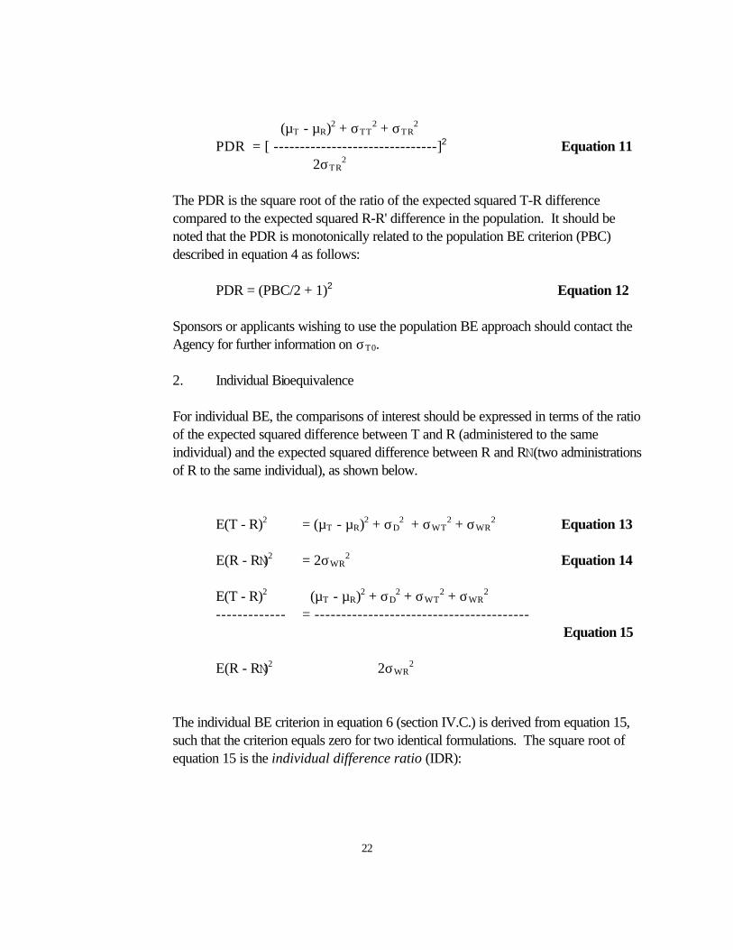
(µT - µR)2 + σTT2 + σTR

2

PDR = [ -------------------------------]2 Equation 11 2σTR

2

The PDR is the square root of the ratio of the expected squared T-R differencecompared to the expected squared R-R' difference in the population. It should benoted that the PDR is monotonically related to the population BE criterion (PBC)described in equation 4 as follows:

PDR = (PBC/2 + 1)2 Equation 12

Sponsors or applicants wishing to use the population BE approach should contact theAgency for further information on σT0.


For individual BE, the comparisons of interest should be expressed in terms of the ratioof the expected squared difference between T and R (administered to the sameindividual) and the expected squared difference between R and RN (two administrationsof R to the same individual), as shown below.

E(T - R)2 = (µT - µR)2 + σD2 + σWT

2 + σWR2 Equation 13

E(R - RN)2 = 2σWR2 Equation 14

E(T - R)2 (µT - µR)2 + σD2 + σWT

2 + σWR2

------------- = ----------------------------------------Equation 15

E(R - RN)2 2σWR2

The individual BE criterion in equation 6 (section IV.C.) is derived from equation 15,such that the criterion equals zero for two identical formulations. The square root ofequation 15 is the individual difference ratio (IDR):

23

(µT - µR)2 + σD2 + σWT

2 + σWR2

IDR = [ ----------------------------------------]2 Equation 16 2σWR

2

The IDR is the square root of the ratio of the expected squared T-R differencecompared to the expected squared R-R' difference within an individual. The IDR ismonotonically related to the individual BE criterion (IBC) described in equation 6 asfollows:

IDR = (IBC/2 + 1)2 Equation 17

This guidance recommends that σW0 = 0.2, based on the consideration of the maximumallowable IDR of 1.25.4

B. θθ P and θθ I

The determination of θP and θI should be based on the consideration of average BE criterionand the addition of variance terms to the population and individual BE criterion, as expressed bythe formula below.

average BE limit + variance factorθ = -----------------------------------------------

variance


(ln1.25)2 + εP

θP = -------------------------- Equation 18 σT0

2

The value of εP for population BE is guided by the consideration of the variance term(σTT

2 - σTR2) added to the average BE criterion. Sponsors or applicants wishing to use

the population BE approach should contact the Agency for further information on εP

and θP.

4 The IDR upper bound of 1.25 is drawn from the currently used upper BE limit of 1.25 for the average BE

criterion.

24


(ln1.25)2 + εI

θI = ----------------------- Equation 19 σW0

2

The value of εI for individual BE is guided by the consideration of the estimate ofsubject-by-formulation interaction (σD) as well as the difference in within-subjectvariability (σWT

2 - σWR2) added to the average BE criterion. The recommended

allowance for the variance term (σWT2 - σWR

2) is 0.02. In addition, this guidancerecommends a σD

2 allowance of 0.03. The magnitude of σD is associated with thepercentage of individuals whose average T to R ratios lie outside 0.8-1.25. It isestimated that if σD = 0.1356, ~10% of the individuals would have their average ratiosoutside 0.8-1.25, even if µT - µR= 0. When σD = 0.1741, the probability is ~20%.

Accordingly, on the basis of consideration for both σD and variability (σWT2 - σWR

2) inthe criterion, this guidance recommends that εI = 0.05.

25

APPENDIX B

Choice of Specific Replicated Crossover Designs

Appendix B describes why FDA prefers replicated crossover designs with only two sequences, andwhy we recommend the specific designs described in section V.A of this guidance.

1. Reasons Unrelated to Carryover Effects

Each unique combination of sequence and period in a replicated crossover design can be called a cell ofthe design. For example, the two-sequence, four-period design recommended insection V.A.1 has 8 cells. The four-sequence, four-period design below has 16 cells.

Period

1 2 3 4

1 T R R T

2 R T T RSequence

3 T T R R

4 R R T T

The total number of degrees-of-freedom attributable to comparisons among the cells is just the numberof cells minus one (unless there are cells with no observations).

The fixed effects that are usually included in the statistical analysis are sequence, period, and treatment(i.e., formulation). The number of degrees-of-freedom attributable to each fixed effect is generally equalto the number of levels of the effect, minus one. Thus, in the case of the two-sequence, four-perioddesign recommended in section V.A.1, there would be 2-1=1 degree-of-freedom due to sequence, 4-1=3 degrees-of-freedom due to period, and 2-1=1 degree-of-freedom due to treatment, for a total of1+3+1=5 degrees-of-freedom due to the three fixed effects. Because these 5 degrees-of-freedom donot account for all 7 degrees-of-freedom attributable to the eight cells of the design, the fixed effectsmodel is not saturated. There could be some controversy as to whether a fixed effects model thataccounts for more or all of the degrees-of-freedom due to cells (i.e., a more saturated fixed effectsmodel) should be used. For example, an effect for sequence-by-treatment interaction might be includedin addition to the three main effects — sequence, period, and treatment. Alternatively, a sequence-by-

26

period interaction effect might be included, which would fully saturate the fixed effects model.

If the replicated crossover design has only two sequences, use of only the three main effects (sequence,period, and treatment) in the fixed effects model or use of a more saturated model makes little differenceto the results of the analysis, provided there are no missing observations and the study is carried out inone group of subjects. The least squares estimate of µT-µR will be the same for the main effects modeland for the saturated model. Also, the method of moments (MM) estimators of the variance terms inthe model used in some approaches to assessment of population and individual BE (see Appendix H),which represent within-sequence comparisons, are generally fully efficient regardless of whether themain effects model or the saturated model is used.

If the replicated crossover design has more than two sequences, these advantages are no longerpresent. Main effects models will generally produce different estimates of µT-µR than saturated models(unless the number of subjects in each sequence is equal), and there is no well-accepted basis forchoosing between these different estimates. Also, MM estimators of variance terms will be fully efficientonly for saturated models, while for main effects models fully efficient estimators would have to includesome between-sequence components, complicating the analysis. Thus, use of designs with only twosequences minimizes or avoids certain ambiguities due to the method of estimating variances or due tospecific choices of fixed effects to be included in the statistical model.

2. Reasons Related to Carryover Effects

One of the reasons to use the four-sequence, four-period design described above is that it is thought tobe optimal if carryover effects are included in the model. Similarly, the two-sequence, three-perioddesign

Period

1 2 3

1 T R RSequence

2 R T T

is thought to be optimal among three-period replicated crossover designs. Both of these designs arestrongly balanced for carryover effects, meaning that each treatment is preceded by each othertreatment and itself an equal number of times.

With these designs, no efficiency is lost by including simple first-order carryover effects in the statisticalmodel. However, if the possibility of carryover effects is to be considered in the statistical analysis ofBE studies, the possibility of direct-by-carryover interaction should also be considered. If direct-by-

27

carryover interaction is present in the statistical model, these favored designs are no longer optimal. Indeed, the TRR/RTT design does not permit an unbiased within-subject estimate of µT-µR in thepresence of general direct-by-carryover interaction.

The issue of whether a purely main effects model or a more saturated model should be specified, asdescribed in the previous section, also is affected by possible carryover effects. If carryover effects,including direct-by-carryover interaction, are included in the statistical model, these effects will bepartially confounded with sequence-by-treatment interaction in four-sequence or six-sequencereplicated crossover designs, but not in two-sequence designs.

In the case of the four-period and three-period designs recommended in section V.A.1, the estimate ofµT-µR, adjusted for first-order carryover effects including direct-by-carryover interaction, is as efficientor more efficient than for any other two-treatment replicated crossover designs.

3. Two-Period Replicated Crossover Designs

For the majority of drug products, two-period replicated crossover designs such as the Balaam design(which uses the sequences TR, RT, TT, and RR) should be avoided for individual BE because subjectsin the TT or RR sequence do not provide any information on subject-by-formulation interaction. However, the Balaam design may be useful for particular drug products (e.g., a long half-life drug forwhich a two-period study would be feasible but a three- or more period study would not).

28

APPENDIX C

Sample Size Determination

Sample sizes for average BE should be obtained using published formulas. Sample sizes for populationand individual BE should be based on simulated data. The simulations should be conducted using adefault situation allowing the two formulations to vary as much as 5% in average BA with equalvariances and certain magnitude of subject-by-formulation interaction. The study should have 80 or90% power to conclude BE between these two formulations. Sample size also depends on themagnitude of variability and the design of the study. Variance estimates to determine the number ofsubjects for a specific drug can be obtained from the biomedical literature and/or pilot studies.

Tables 1-4 below give sample sizes for 80% and 90% power using the specified study design, given aselection of within-subject standard deviations (natural log scale), between-subject standard deviations(natural log scale), and subject-by-formulation interaction, as appropriate.

Table 1

Average BioequivalenceEstimated Numbers of Subjects

∆∆ =0.05

80% Power 90% PowerσW T = σD 2P 4P 2P 4P0.15 0.01 12 6 16 8

0.10 14 10 18 120.15 16 12 22 16

0.23 0.01 24 12 32 160.10 26 16 36 200.15 30 18 38 24

0.30 0.01 40 20 54 280.10 42 24 56 300.15 44 26 60 34

0.50 0.01 108 54 144 720.10 110 58 148 760.15 112 60 150 80

Note: 1. Results for two-period designs use method of Diletti et al. (Diletti 1991).2. Results for four-period designs use relative efficiency data of Liu (Liu 1995).

29

Table 2

Population BioequivalenceFour-Period Design (RTRT/TRTR)

Estimated Numbers of SubjectsεP =0.02, ∆∆ =0.05

σWR = σWT σBR=σBT 80% Power 90% Power0.15 0.15 18 22

0.30 24 32

0.23 0.23 22 28

0.46 24 32

0.30 0.30 22 28

0.60 26 34

0.50 0.50 22 28

1.00 26 34

Note: Results for population BE are approximate from simulation studies(1,540 simulations for each parameter combination), assuming two-sequence,four-period trials with a balanced design across sequences.

30

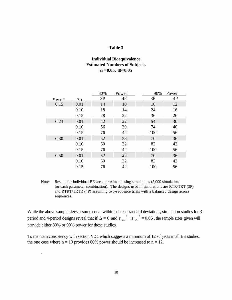
Table 3

Individual BioequivalenceEstimated Numbers of Subjects

εI =0.05, ∆∆ =0.05

80% Power 90% PowerσW T = σD 3P 4P 3P 4P0.15 0.01 14 10 18 12

0.10 18 14 24 160.15 28 22 36 26

0.23 0.01 42 22 54 300.10 56 30 74 400.15 76 42 100 56

0.30 0.01 52 28 70 360.10 60 32 82 420.15 76 42 100 56

0.50 0.01 52 28 70 360.10 60 32 82 420.15 76 42 100 56

Note: Results for individual BE are approximate using simulations (5,000 simulationsfor each parameter combination). The designs used in simulations are RTR/TRT (3P)and RTRT/TRTR (4P) assuming two-sequence trials with a balanced design acrosssequences.

While the above sample sizes assume equal within-subject standard deviations, simulation studies for 3-

period and 4-period designs reveal that if 0∆ = and 2 2 0.05WT WRσ σ− = , the sample sizes given will

provide either 80% or 90% power for these studies.

To maintain consistency with section V.C, which suggests a minimum of 12 subjects in all BE studies,the one case where n = 10 provides 80% power should be increased to n = 12.

.

31

Table 4

Individual BioequivalenceEstimated Numbers of Subjects

εI =0.05, ∆∆ =0.10With Constraint on ∆∆ (0.8 ≤≤ exp(∆∆ ) ≤≤ 1.25)

80% Power 90% PowerσW T = σD 4P 4P0.30 0.01 30 40

0.10 36 480.15 42 56

0.50 0.01 34 460.10 36 480.15 42 56

Note: Results for individual BE are approximate using simulations (5,000 simulationsfor each parameter combination). The designs used in simulations are RTRT/TRTR (4P),assuming two-sequence trials with a balanced design across sequences. When ∆=0.05,sample sizes remain the same as given in Table 3. This is because the studies are alreadypowered for variance estimation and inference, and therefore, a constraint on the pointestimate of ∆ has little influence on the sample size for small values of ∆.

32

APPENDIX D

Rationale for Logarithmic Transformation of Pharmacokinetic Data

A. Clinical Rationale

The FDA Generic Drugs Advisory Committee recommended in 1991 that the primary comparison ofinterest in a BE study is the ratio, rather than the difference, between average parameter data from the Tand R formulations. Using logarithmic transformation, the general linear statistical model employed inthe analysis of BE data allows inferences about the difference between the two means on the log scale,which can then be retransformed into inferences about the ratio of the two averages (means or medians)on the original scale. Logarithmic transformation thus achieves a general comparison based on the ratiorather than the differences.

B. Pharmacokinetic Rationale

Westlake observed that a multiplicative model is postulated for pharmacokinetic measures in BA/BEstudies (i.e., AUC and Cmax, but not Tmax) (Westlake 1973 and 1988). Assuming that elimination ofthe drug is first-order and only occurs from the central compartment, the following equation holds afteran extravascular route of administration:

AUC0-4 = FD/CL Equation 20

= FD/(VKe) Equation 21

where F is the fraction absorbed, D is the administered dose, and FD is the amount of drug absorbed. CL is the clearance of a given subject that is the product of the apparent volume of distribution (V) andthe elimination rate constant (Ke).5 The use of AUC as a measure of the amount of drug absorbed 5 Note that a more general equation can be written for any multicompartmental model as

AUC0-� = FD/Vdß λn Equation 22 where Vdß is the volume of distribution relating drug concentration in plasma or blood to the amount of drug in thebody during the terminal exponential phase, and λn is the terminal slope of the concentration-time curve.

33

involves a multiplicative term (CL) that might be regarded as a function of the subject. For this reason,Westlake contends that the subject effect is not additive if the data are analyzed on the original scale ofmeasurement.

Logarithmic transformation of the AUC data will bring the CL (VKe) term into the following equation inan additive fashion:

lnAUC0-4 = ln F + ln D - ln V - ln Ke Equation 23

Similar arguments were given for Cmax. The following equation applies for a drug exhibiting onecompartmental characteristics:

Cmax = (FD/V) x e-ke*Tmax Equation 24

where again F, D and V are introduced into the model in a multiplicative manner. However, afterlogarithmic transformation, the equation becomes

lnCmax = ln F + ln D - ln V - KeTmax Equation 25

Thus, log transformation of the Cmax data also results in the additive treatment of the V term.

34

APPENDIX E

SAS Program Statements for Average BE Analysis ofReplicated Crossover Studies

The following illustrates an example of program statements to run the average BE analysis usingPROC MIXED in SAS version 6.12, with SEQ, SUBJ, PER, and TRT identifying sequence,subject, period, and treatment variables, respectively, and Y denoting the response measure (e.g.,log(AUC), log(Cmax)) being analyzed:

PROC MIXED;CLASSES SEQ SUBJ PER TRT;MODEL Y = SEQ PER TRT/ DDFM=SATTERTH;RANDOM TRT/TYPE=FA0(2) SUB=SUBJ G;REPEATED/GRP=TRT SUB=SUBJ;ESTIMATE 'T vs. R' TRT 1 -1/CL ALPHA=0.1;

The Estimate statement assumes that the code for the T formulation precedes the code for the Rformulation in sort order (this would be the case, for example, if T were coded as 1 and R werecoded as 2). If the R code precedes the T code in sort order, the coefficients in the Estimatestatement would be changed to -1 1.

In the Random statement, TYPE=FA0(2) could possibly be replaced by TYPE=CSH. Thisguidance recommends that TYPE=UN not be used, as it could result in an invalid (i.e., not non-negative definite) estimated covariance matrix.

Additions and modifications to these statements can be made if the study is carried out in more thanone group of subjects.

35

APPENDIX F

Method for Statistical Test of Population Bioequivalence Criterion

Four-Period Crossover Designs

Appendix F describes a method for using the population BE criterion (see section IV.B, equations 4and 5). The procedure involves the computation of a test statistic that is either positive (does notconclude population BE) or negative (concludes population BE).

Consider the following statistical model which assumes a four-period design with equal replication ofT and R in each of s sequences with an assumption of no (or equal) carryover effects (equalcarryovers go into the period effects)

ijkl k ikl ijk ijklY µ γ δ ε= + + +

where 1,i s= K indicates sequence, 1, ij n= K indicates subject within sequence i, k = R, T

indicates treatment, l =1, 2 indicates replicate on treatment k for subjects within sequence i. ijklY is

the response of replicate l on treatment k for subject j in sequence i , iklγ represents the fixed

effect of replicate l on treatment k in sequence i , ijkδ is the random subject effect for subject j in

sequence i on treatment k , and ijklε is the random error for subject j within sequence i on

replicate l of treatment k . The ijklε ’s are assumed to be mutually independent and identically

distributed as

ε ijkl ~ N(0, σWk2 )

for 1,i s= K , 1, ij n= K , k = R, T, and l = 1, 2. Also, the random subject effects

( ),ij R ijR T ijTµ δ µ δ ′= + +δδ are assumed to be mutually independent and distributed as

2

2 2~ ,R BR BT BR

ijT BT BR BT

Nµ σ ρσ σµ ρσ σ σ

δδ .

The following constraint is applied to the nuisance parameters to avoid overparameterization of themodel for k=R, T:

36

2

1 1

0s

ikli l

γ= =

=∑ ∑

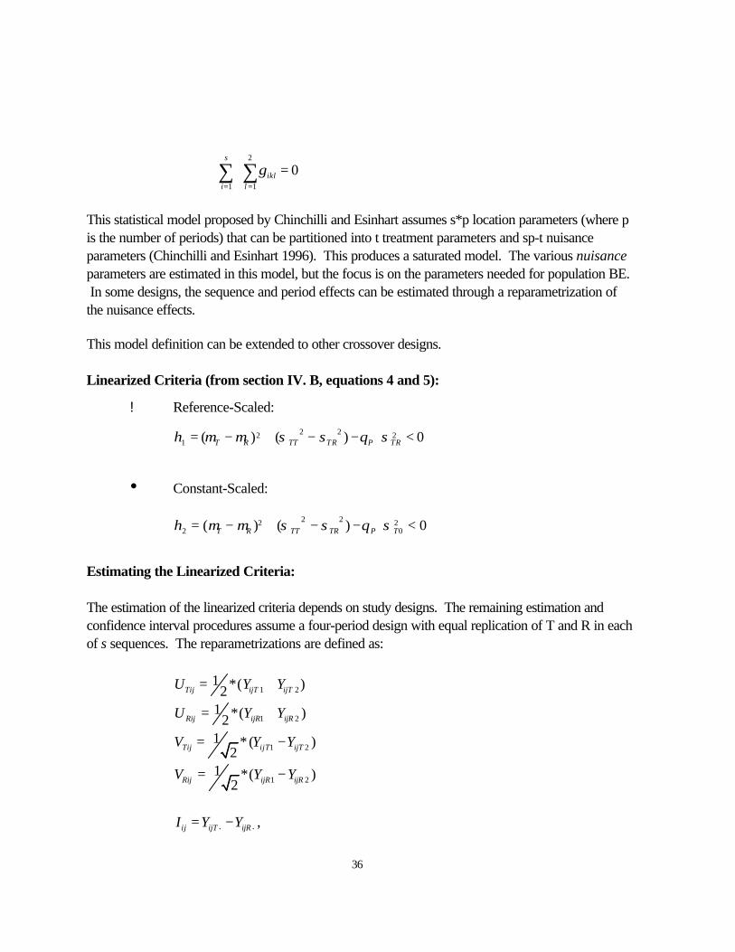
This statistical model proposed by Chinchilli and Esinhart assumes s*p location parameters (where pis the number of periods) that can be partitioned into t treatment parameters and sp-t nuisanceparameters (Chinchilli and Esinhart 1996). This produces a saturated model. The various nuisanceparameters are estimated in this model, but the focus is on the parameters needed for population BE. In some designs, the sequence and period effects can be estimated through a reparametrization ofthe nuisance effects.

This model definition can be extended to other crossover designs.

Linearized Criteria (from section IV. B, equations 4 and 5):

! Reference-Scaled:

2 22 21 ( ) ( ) 0T R TT TR P TRη µ µ σ σ θ σ= − + − − ⋅ <

• Constant-Scaled:

2 22 22 0( ) ( ) 0T R TT TR P Tη µ µ σ σ θ σ= − + − − ⋅ <

Estimating the Linearized Criteria:

The estimation of the linearized criteria depends on study designs. The remaining estimation andconfidence interval procedures assume a four-period design with equal replication of T and R in eachof s sequences. The reparametrizations are defined as:

1 21 *( )2Tij ijT ijTU Y Y= +

1 21 *( )2Rij ijR ijRU Y Y= +

1 21 * ( )

2Tij ijT ijTV Y Y= −

1 21 *( )

2Rij ijR ijRV Y Y= −

ij ijT ijRI Y Y• •

= − ,

37

for 1, ,i s= K and 1, , ij n= K , where

( )1 2

1

2ijT ijT ijTY Y Y= +g and ( )1 2

1

2ijR ijR ijRY Y Y= +g .

Compute the formulation means pooling across sequences:

1

1 , ,s

i kki

Y k R Tsµ∧

⋅ ⋅=

= =∑ and ˆ ˆ ˆT Rµ µ∆ = −

where

2

1 1

1

2

1 in

i k ijklj li

Y Yn⋅ ⋅

= =

= ∑ ∑ .

Compute the variances of , , ,Tij Rij Tij RijU U V V , pooling across sequences, and denote these variance

estimates by , , ,T R T RMU MU MV MV , respectively. Specifically,

( )2

1 1

1 i

T

ns

T Tij Tii jU

MU U Un = =

= −∑∑

( )2

1 1

1 i

T

ns

T Tij Tii jV

MV V Vn = =

= −∑∑

( )2

1 1

1 i

R

ns

R Rij Rii jU

MU U Un = =

= −∑∑

( )2

1 1

1 i

R

ns

R Rij Rii jV

MV V Vn = =

= −∑∑

1T R T R

s

I U U V V ii

n n n n n n s=

= = = = = − ∑

Then, the linearized criteria are estimated by:

! Reference-Scaled:

2

1 0.5 (1 ) [ 0.5 ]T T P R RMU MV MU MVη θ∧ ∧

= ∆ + + ⋅ − + ⋅ + ⋅

38


2

02 0.5 (1) [ 0.5 ]T T R R P TMU MV MU MVη θ σ∧ ∧

= ∆ + + ⋅ − ⋅ + ⋅ − ⋅

95% Upper Confidence Bounds for Criteria:

The table below illustrates the construction of a ( )1 α− level upper confidence bound based on the

two-sequence, four-period design, for the reference-scaled criterion, 1η∧

. Use α=0.05 for a 95%

upper confidence bound.

Hq= Confidence Bound Eq= Point Estimate Uq=(Hq- Eq)2

212

1

21

1 ,1 s

D i Ii

n sH t n Msα

∧−

=− −

= + ∆ ∑

2

DE∧

= ∆ DU

( ),

2

11

n s

n s EH

αχ −

− ⋅=

1TMU E= 1U

,2

( ) 22

n s

n s EH

αχ −

− ⋅= 0.5 2TMV E⋅ = 2U

,12

( ) 33

n s

n s E rsH rs

αχ − −

− ⋅= ( )1 3p RMU E rsθ− + = 3U rs

,12

( ) 44

n s

n s E rsH rs

αχ − −

− ⋅= (1 ) 0.5 4p RMV E rsθ− + ⋅ ⋅ =

4U rs

( )1

12

q qH E Uη = +∑ ∑

( )1

12

q qH E Uη = +∑ ∑ is the upper 95% confidence bound for 1η∧

. Note 1

s

ii

n n=

= ∑ , where s is

the number of sequences, in is the number of subjects per sequence, and 2,n sαχ − is from the

cumulative distribution function of the chi-square distribution with n s− degrees of freedom, i.e.

39

2 2,Pr ( )n s n sα αχ χ− −≤ = . The confidence bound for 2η

∧ is computed similarly, adjusting the

constants associated with the variance components where appropriate (in particular, the constantassociated with MUR and MVR).


212

1

21

1 ,1 s

D i Ii

n sH t n Msα

∧−

=− −

= + ∆ ∑

2

DE∧

= ∆ DU

( ),

2

11

n s

n s EH

αχ −

− ⋅=

1TMU E= 1U

,2

( ) 22

n s

n s EH

αχ −

− ⋅= 0.5 2TMV E⋅ = 2U

( ),1

2

33

n s

n s E csH cs

αχ − −

−= 1 3RMU E cs− ⋅ = 3U cs

( ),1

2

44

n s

n s E csH cs

αχ − −

−=

0.5 4RMV E cs− ⋅ = 4U cs

( )2

12 2

0q P T qH E Uη θ σ= − ⋅ +∑ ∑

Using the mixed-scaling approach, to test for population BE, compute the 95% upper confidencebound of either the reference-scaled or constant-scaled linearized criterion. The selection of eitherreference-scaled or constant-scaled approach depends on the study estimate of total standard

deviation of the reference product (estimated by 1

2[ 0.5 ]R RMU MV+ ⋅ in the four-period design). If

the study estimate of standard deviation is 0Tσ≤ , the constant-scaled criterion and its associated

confidence interval should be computed. Otherwise, the reference-scaled criterion and itsconfidence interval should be computed. The procedure for computing each of the confidencebounds is described above. If the upper confidence bound for the appropriate criterion is negativeor zero, conclude population BE. If the upper bound is positive, do not conclude population BE.

40

APPENDIX G

Method for Statistical Test of Individual Bioequivalence Criterion

Appendix G describes a method for using the individual BE criterion (see section IV.C, equations 6and 7). The procedure (Hyslop, Hsuan, and Holder 2000) involves the computation of a teststatistic that is either positive (does not conclude individual BE) or negative (concludes individualBE).

Consider the following statistical model that assumes a four-period design with equal replication of Tand R in each of s sequences with an assumption of no (or equal) carryover effects (equalcarryovers go into the period effects)

i j k l k i k l i j k i j k lY µ γ δ ε= + + +

where 1,i s= K indicates sequence, 1, ij n= K indicates subject within sequence i, k = R, T

indicates treatment, l=1, 2 indicates replicate on treatment k for subjects within sequence i. ijklY is the

response of replicate l on treatment k for subject j in sequence i , iklγ represents the fixed effect

of replicate l on treatment k in sequence i , ijkδ is the random subject effect for subject j in

sequence i on treatment k , and ijklε is the random error for subject j within sequence i on

replicate l of treatment k . The ijklε ’s are assumed to be mutually independent and identically

distributed as

ε ijkl ~ N(0, σWk2 )

for 1,i s= K , 1, ij n= K , k = R, T, and l = 1, 2. Also, the random subject effects

( ),ij R ijR T ijTµ δ µ δ ′= + +δδ are assumed to be mutually independent and distributed as

2

2 2~ ,R BR BT BR

ijT BT BR BT

Nµ σ ρσ σµ ρσ σ σ

δδ .

The following constraint is applied to the nuisance parameters to avoid overparameterization of themodel for k = R, T:

41

2

1 1

0s

ikli l

γ= =

=∑ ∑

This statistical model proposed by Chinchilli and Esinhart assumes s*p location parameters (where pis the number of periods) that can be partitioned into t treatment parameters and sp-t nuisanceparameters (Chinchilli and Esinhart, 1996). This produces a saturated model. The various nuisanceparameters are estimated in this model, but the focus is on the parameters needed for individual BE. In some designs, the sequence and period effects can be estimated through a reparametrization of thenuisance effects.

This model definition can be extended to other crossover designs.

Linearized Criteria (from section IV. C, equations 6 and 7) :

• Reference-Scaled:

2 22 2 21 ( ) ( ) 0T R D WT WR I WRη µ µ σ σ σ θ σ= − + + − − ⋅ <


2 22 2 22 0( ) ( ) 0T R D WT WR I Wη µ µ σ σ σ θ σ= − + + − − ⋅ <

Estimating the Linearized Criteria:

The estimation of the linearized criteria depends on study designs. The remaining estimation andconfidence interval procedures assume a four-period design with equal replication of T and R in eachof s sequences. The reparametrizations are defined as:

ij ijT ijRI Y Y• •

= −

1 2ij ijT ijTT Y Y= −

1 2ij ijR ijRR Y Y= −

for 1, ,i s= K and 1, , ij n= K , where

42

( )1 2

1

2ijT ijT ijTY Y Y= +g and ( )1 2

1

2ijR ijR ijRY Y Y= +g

Compute the formulation means, and the variances of ijI , ijT , and ijR , pooling across sequences,

and denote these variance estimates by IM , TM , and RM , respectively, where

1

1 , ,s

i kki

Y k R Tsµ∧

⋅ ⋅=

= =∑ and ˆ ˆ ˆT Rµ µ∆ = −

2

1 1

1

2

1 in

i k ijklj li

Y Yn⋅ ⋅

= =

= ∑ ∑

( )22

1 1

1 ins

II ij ii jI

M I In

σ∧

= =

= = −∑∑

1

s

I T R ii

n n n n s=

= = = − ∑

( )22

1 1

1ˆ2

ins

T WT ij ii jT

M T Tn

σ= =

= = −∑∑

( )22

1 1

1ˆ2

ins

R WR ij ii jR

M R Rn

σ= =

= = −∑∑ .

Then, the linearized criteria are estimated by:

• Reference-Scaled:

2

1 0.5 (1.5 )I T I RM M Mη θ∧ ∧

= ∆ + + ⋅ − + ⋅


2

202 0.5 1.5I T R I WM M Mη θ σ

∧ ∧= ∆ + + ⋅ − ⋅ − ⋅

and the subject-by-formulation interaction variance component can be estimated by:

43

( )2 2 2 21ˆ ˆ ˆ ˆ2D I WT WRσ σ σ σ= − +

95% Upper Confidence Bounds for Criteria:

The table below illustrates the construction of a ( )1 α− level upper confidence bound based on the

two-sequence, four-period design, for the reference-scaled criterion, 1η∧

. Use α=0.05 for a 95%

upper confidence bound.


212

1

21

1 ,1 s

D i Ii

n sH t n Msα

∧−

=− −

= + ∆ ∑

2

DE∧

= ∆ DU

2 ,

( ) I

n sI

n s MH

αχ −

− ⋅= I IE M= IU

2,

0.5 ( ) T

n sT

n s MH

αχ −

⋅ − ⋅= 0.5T TE M= ⋅ TU

( )2

1 ,

1.5 ( )I R

n sR

n s MH

α

θχ − −

− + ⋅ − ⋅= ( )1.5R I RE Mθ= − + ⋅ RU

( )1

12

q qH E Uη = +∑ ∑

where 1

s

ii

n n=

= ∑ , s is the number of sequences, and 2,n sαχ − is from the cumulative distribution

function of the chi-square distribution with n s− degrees of freedom, i.e. 2 2,P r ( )n s n sα αχ χ− −≤ = .

Then, ( )1

12

q qH E Uη = +∑ ∑ is the upper 95% confidence bound for 1η∧

. The confidence bound

for 2η∧

is computed similarly, adjusting the constants associated with the variance components where

appropriate (in particular, the constant associated with MR).

44


212

1

21

1 ,1 s

D i Ii

n sH t n Msα

∧−

=− −

= + ∆ ∑

2

DE∧

= ∆ DU

2 ,

( ) I

n sI

n s MH

αχ −

− ⋅= I IE M= IU

2,

0.5 ( ) T

n sT

n s MH

αχ −

⋅ − ⋅= 0.5T TE M= ⋅ TU

( )21 ,

1.5 ( ) R

n sR

n s MH

αχ − −

− ⋅ − ⋅= ( )1.5R RE M= − ⋅ RU

( )2

12 2

0q I W qH E Uη θ σ= − ⋅ +∑ ∑

Using the mixed-scaling approach, to test for individual BE, compute the 95% upper confidencebound of either the reference-scaled or constant-scaled linearized criterion. The selection of eitherreference-scaled or constant-scaled criterion depends on the study estimate of within-subjectstandard deviation of the reference product. If the study estimate of standard deviation is 0Wσ≤ , the

constant-scaled criterion and its associated confidence interval should be computed. Otherwise, thereference-scaled criterion and its confidence interval should be computed. The procedure forcomputing each of the confidence bounds is described above. If the upper confidence bound for theappropriate criterion is negative or zero, conclude individual BE. If the upper bound is positive, donot conclude individual BE.

This guidance recommends that sponsors use either reference-scaling or constant-scaling at thechangeover point (see section VII.D, Discontinuity). To test for individual BE, compute the 95%upper confidence bounds of both reference-scaled and constant-scaled linearized criteria. Theprocedure for computing these confidence bounds is described above. If the upper bound of eithercriterion is negative or zero (either

1 2orH Hη η ), conclude individual BE. If the upper bounds of

both criteria are positive, do not conclude individual BE.

45

APPENDIX H

Variance Estimation

Relatively simple unbiased estimators, the method of moments (MM) or the restricted maximumlikelihood (REML) method, can be used to estimate the mean and variance parameters in theindividual BE approach. A key distinction between the REML and MM methods relates todifferences in estimating variance terms. The REML method estimates each of the three variances,σD

2, σW R2, σW T

2, separately and then combines them in the individual BE criterion. The REMLestimate of σD

2 is found from estimates of σBR2, σBT

2, and the correlation, ρ. The MM approachis to estimate the sum of the variance terms in the numerator of the criterion, σD

2 + σW T2 - σW R

2,and does not necessarily estimate each component separately. One consequence of this differenceis that the MM estimator of σD

2 is unbiased but could be negative. The REML approach can alsolead to negative estimates, but if the covariance matrix of the random effects is forced to be aproper covariance matrix, the estimate of σD

2 can be made to be non-negative. This forced non-negativity has the effect of making the estimate positively biased and introduces a small amount ofconservatism to the confidence bound. The REML method can be used in special cases (e.g., whensubstantial missing data are present). In addition, the MM approaches have not yet been adaptedto models that allow assessment of carryover effects.

Statistical Approaches to Establishing Bioequivalence€¦ · Guidance for Industry Statistical...

Documents

Transcript of Statistical Approaches to Establishing Bioequivalence€¦ · Guidance for Industry Statistical...