Statistical and Economic Methodsfor Evaluating Exchange Rate Predictability∗

Pasquale Della CorteImperial College London

Ilias TsiakasUniversity of Guelph

October 2011

Abstract

This chapter provides a comprehensive review of the statistical and economic methods usedfor evaluating out-of-sample exchange rate predictability. We illustrate these methods by assess-ing the forecasting performance of a set of widely used empirical exchange rate models usingmonthly returns on nine major US dollar exchange rates. We find that empirical models basedon uncovered interest parity, purchasing power parity and the asymmetric Taylor rule performbetter than the random walk in out-of-sample forecasting using both statistical and economiccriteria. We also confirm that conditioning on monetary fundamentals does not generate out-of-sample economic value. Finally, combined forecasts formed using a variety of model averagingmethods perform better than individual empirical models. These results are robust to reasonablyhigh transaction costs, the choice of numeraire and the exclusion of any one currency from theinvestment opportunity set.

Keywords: Exchange Rates; Out-of-Sample Predictability; Mean Squared Error; EconomicValue; Combined Forecasts.

JEL Classification: F31; F37; G11; G17.

∗This paper is forthcoming as a chapter in the Handbook of Exchange Rates. The authors are grateful to Lu-cio Sarno and an anonymous referee for useful comments. Contact details : Pasquale Della Corte, Finance Group,Imperial College Business School, Imperial College London, 53 Prince’s Gate, London SW7 2AZ, UK. Email:p.dellacorte@imperial.ac.uk; Ilias Tsiakas, Department of Economics and Finance, University of Guelph, Guelph, On-tario N1G 2W1, Canada. Email: itsiakas@uoguelph.ca.

1 Introduction

Exchange rate fluctuations are regularly monitored with great interest by policy makers, practitioners

and academics. It is not surprising, therefore, that exchange rate predictability has long been at

the top of the research agenda in international finance. Starting with the seminal contribution of

Meese and Rogoff (1983), a large body of empirical research finds that models which condition on

economically meaningful variables do not provide reliable exchange rate forecasts. This has lead

to the prevailing view that exchange rates follow a random walk and hence are not predictable,

especially at short horizons.

Several well known puzzles in foreign exchange (FX) are responsible for this view. First, the

“exchange rate disconnect puzzle” concerns the empirical disconnect between exchange rate move-

ments and economic fundamentals such as money supply and real output (e.g., Mark, 1995; Cheung,

Chinn and Pascual, 2005; Rogoff and Stavrakeva, 2008). Second, the “forward premium puzzle”

implies that on average the interest differential is not offset by a commensurate depreciation of the

investment currency, which is an empirical violation of uncovered interest rate parity. As a result,

borrowing in low-interest rate currencies and investing in high-interest rate currencies forms the basis

of the widely used carry trade strategy in active currency management (e.g., Fama, 1984; Burnside,

Eichenbaum, Kleshchelski and Rebelo, 2011; Brunnermeier, Nagel and Pedersen, 2009; and Della

Corte, Sarno and Tsiakas, 2009). Third, there is extensive evidence that purchasing power parity

holds in the long run (e.g., Lothian and Taylor, 1996).

A recent contribution by Engel and West (2005) provides a possible resolution to the diffi culty of

tying exchange rates to economic fundamentals. Specifically, Engel andWest (2005) show analytically

that exchange rates can be consistent with present-value asset pricing models and still manifest near-

random walk behaviour if two conditions are met: (i) fundamentals are integrated of order one, and

(ii) the discount factor for future fundamentals is near one.1

A model that is nested by the Engel and West (2005) present value relation is a variant of the

Taylor (1993) rule used for exchange rate determination. The Taylor rule postulates that the central

bank adjusts the short-run nominal interest rate in response to changes in inflation, the output gap

and the exchange rate. Using alternative specifications of Taylor rule fundamentals, Molodtsova and

Papell (2009) provide strong evidence of short-horizon exchange rate predictability, and hence offer

renewed hope for empirical success in this literature. In short, one way to summarize the state of

the literature is that it has come full circle: from the Meese and Rogoff (1983) “no predictability

at short horizons,” to the Mark (1995) “predictability at long but not at short horizons,” to the

Cheung, Chinn and Pascual (2005) “no predictability at any horizon,”to finally the Molodtsova and

1The assumption of integrated fundamentals of order one is widely accepted in the literature. The assumption thatthe discount factor is close to one has been empirically validated by Sarno and Sojli (2009).

1

Papell (2009) “predictability at short horizons with Taylor rule fundamentals.”

This chapter aims at connecting these related literatures by providing a comprehensive review

of the statistical and economic methods used for evaluating exchange rate predictability, especially

out of sample. We assess the short-horizon forecasting performance of a set of widely used empirical

exchange rate models that include the random walk model, uncovered interest parity, purchasing

power parity, monetary fundamentals, and symmetric and asymmetric Taylor rules. Our analysis

employs monthly FX data ranging from January 1976 to June 2010 for the 10 most liquid (G10)

currencies in the world: the Australian dollar, Canadian dollar, Swiss franc, Deutsche mark\euro,

British pound, Japanese yen, Norwegian kroner, New Zealand dollar, Swedish kronor and US dollar.2

The vast majority of the FX literature uses a well established statistical methodology for eval-

uating exchange rate predictability. This methodology typically involves statistical tests of the null

hypothesis of equal predictive ability between the random walk benchmark and an alternative em-

pirical exchange rate model. The tests are based on the out-of-sample mean squared error (MSE) of

the forecasts generated by the models. In this chapter, we discuss the main recent contributions to

this methodology.

The most popular method for testing whether the alternative model has a lower MSE than the

benchmark is using the Diebold and Mariano (1995) andWest (1996) statistic. By design, however, all

the models we estimate are nested and this statistic has a non-standard distribution when comparing

forecasts from nested models. Therefore, we focus on the recent inference procedure by Clark and

West (2006, 2007), which accounts for the fact that under the null the MSE from the alternative

model is expected to be greater than that of the RW benchmark because the alternative model

introduces noise into the forecasting process by estimating a parameter vector that is not helpful in

prediction. For a comprehensive statistical evaluation, we also implement the encompassing test of

Clark and McCracken (2001) and the F -statistic of McCracken (2007) using bootstrapped critical

values. Finally, following Campbell and Thompson (2008) and Welch and Goyal (2008) we also

report the out-of-sample R2oos measure and a root MSE difference statistic.

In addition to the extensive literature on statistical evaluation, there is also an emerging line of

research proposing a methodology for assessing the economic value of exchange rate predictability.

A purely statistical analysis of predictability is not particularly informative to an investor as it falls

short of measuring whether there are tangible economic gains from using dynamic forecasts in active

portfolio management. We review this approach based on dynamic asset allocation that is used,

among others, by West, Edison and Cho (1993), Fleming, Kirby and Ostdiek (2001), Marquering

2Note that we will not be discussing two recent approaches to predicting movements in exchange rates: the mi-crostructure approach that conditions on order flow as a measure of net buying pressure for a currency (e.g., Evansand Lyons, 2002, and Rime, Sarno and Sojli, 2010); and (ii) the global imbalances approach (e.g., Gourinchas and Rey,2007, and Della Corte, Sarno and Sestieri, 2011).

2

and Verbeek (2004), Abhyankar, Sarno and Valente (2005), Bandi and Russell (2006), Han (2006),

Bandi, Russell and Zhu (2008), Della Corte, Sarno and Thornton (2008) and Della Corte, Sarno and

Tsiakas (2009, 2011).

We first design an international asset allocation strategy that exposes a US investor purely to

FX risk. The investor builds a portfolio by allocating her wealth between a domestic and a set of

foreign bonds and then uses the exchange rate forecasts from each model to predict the US dollar

return of the foreign bonds. We evaluate the performance of the dynamically rebalanced portfolios

using mean-variance analysis, which allows us to measure how much a risk averse investor is willing

to pay for switching from a portfolio strategy based on the random walk benchmark to an empirical

exchange rate model that conditions on economic fundamentals. In contrast to statistical measures of

forecast accuracy that are computed separately for each exchange rate, the economic value is assessed

for the portfolio generated by a model’s forecasts on all exchange rate returns. This contributes to

our finding that even modest statistical significance in out-of-sample predictive regressions can lead

to large economic benefits for investors.

Our review also includes an assessment of the economic value of combined forecasts. We use a

variety of model averaging methods, some of which generate forecast combinations in a naive ad hoc

manner, some exploit statistical measures of past out-of-sample forecasting performance, and some

that use economic measures of past predictability. All forecast combinations we explore are formed

ex ante using the full universe of individual forecasts of each model for each exchange rate. It is

important to note that the combined forecasts do not require a view of which model is best at any

given time period and therefore provide a way for resolving model uncertainty.

To preview our key results, we find strong statistical and economic evidence against the random

walk benchmark. In particular, empirical exchange rate models based on uncovered interest parity,

purchasing power parity and the asymmetric Taylor rule perform better than the random walk in out-

of-sample prediction using both statistical and economic criteria. We also confirm that conditioning

on monetary fundamentals does not generate out-of-sample economic gains. The worst performing

model is consistently the symmetric Taylor rule. Finally, combined forecasts formed using a variety

of model averaging methods perform even better than individual empirical models. These results

are robust to reasonably high transaction costs, the choice of numeraire and the exclusion of any one

currency from the investment opportunity set.

The remainder of the chapter is organized as follows. In the next section we briefly review

the empirical exchange rate models we estimate and their foundations in asset pricing. Section 3

describes the statistical methods we use for evaluating exchange rate predictability. In Section 4 we

present a general framework for assessing the economic value of forecasting exchange rates for a risk

averse investor with a dynamic mean-variance portfolio allocation strategy. Section 5 explains the

3

construction of combined forecasts using a variety of model averaging methods. Section 6 reports

our empirical results and, finally, Section 7 concludes.

2 Models for Exchange Rate Predictability

In this section we review the empirical models we use for evaluating exchange rate predictability. We

begin by describing the Engel and West (2005) present value model that nests and motivates many

of the predictive regressions we estimate.

2.1 A Present Value Model for Exchange Rates

The Engel and West (2005) model relates the exchange rate to economic fundamentals and the

expected future exchange rate as follows:

st = (1− b) (f1,t + z1,t) + b (f2,t + z2,t) + bEtst+1, (1)

where st is the log of the nominal exchange rate defined as the domestic price of foreign currency,

fi,t (i = 1, 2) are the observed economic fundamentals and zi,t are the unobserved fundamentals that

drive the exchange rate. Note that an increase in st implies a depreciation of the domestic currency.

This is a general asset pricing model that builds on earlier work on pricing stock returns by Campbell

and Shiller (1987, 1988) and West (1988).

Iterating forward and imposing the no-bubbles condition leads to the following present-value

relation:

st = (1− b)∞∑j=0

bjEt (f1,t+j + z1,t+j) + b

∞∑j=0

bjEt (f2,t+j + z2,t+j) . (2)

Engel and West (2005) show that the exchange rate will follow a random walk if the discount factor

b is close to one and either: (1) f1,t + z1,t ∼ I (1) and f2,t + z2,t = 0; or (2) f2,t + z2,t ∼ I (1). Some

other well-known exchange rate models take the general form of Equation (1), and in what follows,

we discuss two examples.

2.1.1 Monetary Fundamentals

Consider first the monetary exchange rate models of the 1970s and 1980s, which assume that the

money market relation is described by:

mt = pt + γyt − αit + vm,t, (3)

where mt is the log of the domestic money supply, pt is the log of the domestic price level, γ > 0

is the income elasticity of money demand, yt is the log of the domestic national income, α > 0 is

the interest rate semi-elasticity of money demand, it is the domestic nominal interest rate and vm,t

4

is a shock to domestic money demand. A similar equation holds for the foreign economy, where the

corresponding variables are denoted by m∗t , p∗t , y

∗t , i∗t and v

∗m,t. We assume that the parameters

{γ, α} of the foreign money demand are identical to the domestic parameters.

The nominal exchange rate is equal to its purchasing power parity (PPP) value plus the real

exchange rate qt:

st = pt − p∗t + qt. (4)

Finally, the interest parity condition is given by:

Etst+1 − st = it − i∗t + ρt, (5)

where ρt is the deviation from the uncovered interest parity (UIP) condition that is based on rational

expectations and risk neutrality. Hence ρt can be interpreted either as an expectational error or a

risk premium.

Using Equations (3) to (5) for the domestic and foreign economies and re-arranging, we get:

st =1

1 + α

[mt −m∗t − γ (yt − y∗t ) + qt −

(vm,t − v∗m,t

)− αρt

]+

α

1 + αEtst+1. (6)

This equation takes the form of the original model in Equation (1), where the discount factor is given

by b = α/1 + α, the observable fundamentals are f1,t = mt −m∗t − γ (yt − y∗t ), and the unobservable

fundamentals are z1,t = qt −(vm,t − v∗m,t

)and z2,t = −ρt.

2.1.2 Taylor Rule

The second model to be nested by the Engel and West (2005) present value relation is the Taylor

(1993) rule, where the home country is assumed to set the short-term nominal interest rate according

to:

it = i+ β1ygt + β2 (πt − π) + vt, (7)

where i is the target short-term interest rate, ygt is the output gap measured as the % deviation

of actual real GDP from an estimate of its potential level, πt is the inflation rate, π is the target

inflation rate and vt is a shock. The Taylor rule postulates that the central bank raises the short-term

nominal interest rate when output is above potential output and/or inflation rises above its desired

level.

The foreign country is assumed to follow a Taylor rule that explicitly targets exchange rates (e.g.,

Clarida, Gali and Gertler, 1998):

i∗t = −β0 (st − st) + i+ β1y∗gt + β2 (π∗t − π) + v∗t , (8)

5

where 0 < β0 < 1 and st is the target exchange rate. For simplicity, we assume that the home and

foreign countries target the same interest rate, i, and the same inflation rate, π. The rule indicates

that the foreign country raises interest rates when its currency depreciates relative to the target.3

We assume that the foreign central bank targets the PPP level of the exchange rate:

st = pt − p∗t . (9)

Taking the difference between the home and foreign Taylor rules, using interest parity (5), sub-

stituting the target exchange rate and solving for st gives:

st =β0

1 + β0(pt − p∗t )−

1

1 + β0

[β1(ygt − y

∗gt

)+ β2 (πt − π∗t ) + vt − v∗t + ρt

]+

1

1 + β0Etst+1. (10)

This equation also has the general form of the present value model in Equation (1), where the discount

factor is b = 1/1 + β0, f1,t = pt − p∗t and z2,t = −[β1(ygt − y

∗gt

)+ β2 (πt − π∗t ) + vt − v∗t + ρt

].

2.2 Predictive Regressions

Our empirical analysis is based on six predictive regressions for exchange rate returns, many of

which are nested and motivated by the Engel and West (2005) present value model. All predictive

regressions have the same linear structure:

∆st+1 = α+ βxt + εt+1, (11)

where ∆st+1 = st+1 − st, α and β are constants to be estimated and εt+1 is a normal error term.

The empirical models differ in the way they specify the economic fundamentals xt that are used to

forecast exchange rate returns.

2.2.1 Random Walk

The first regression is the random walk (RW) with drift model that sets β = 0. Since the seminal

work of Meese and Rogoff (1983), this model has become the benchmark in assessing exchange rate

predictability. The RW model captures the prevailing view in international finance research that

exchange rates are not predictable when conditioning on economic fundamentals, especially at short

horizons.3The argument still follows if the home country also targets exchange rates. It is standard to omit the exchange

rate target from Equation (7) on the interpretation that US monetary policy has essentially ignored exchange rates(see, Engel and West, 2005).

6

2.2.2 Uncovered Interest Parity

The second regression is based on the UIP condition:4

xt = it − i∗t . (12)

UIP is the cornerstone condition for FX market effi ciency. Assuming risk neutrality and rational

expectations, it implies that α = 0, β = 1, and the error term is serially uncorrelated. However,

numerous empirical studies consistently reject the UIP condition (e.g., Hodrick, 1987; Engel, 1996;

Sarno, 2005). As a result, it is a stylized fact that estimates of β tend to be closer to minus unity

than plus unity. This is commonly referred to as the “forward premium puzzle,”which implies that

high-interest currencies tend to appreciate rather than depreciate and forms the basis of the widely

used carry trade strategy in active currency management.5

2.2.3 Purchasing Power Parity

The third regression is based on the PPP hypothesis:

xt = pt − p∗t − st. (13)

The PPP hypothesis states that national price levels should be equal when expressed in a common

currency and is typically thought of as a long-run condition rather than holding at each point in

time (e.g., Rogoff, 1996; and Taylor and Taylor, 2004).

2.2.4 Monetary Fundamentals

The fourth regression conditions on monetary fundamentals (MF):

xt = (mt −m∗t )− (yt − y∗t )− st. (14)

The relation between exchange rates and fundamentals defined in Equation (14) suggests that a

deviation of the nominal exchange rate st+1 from its long-run equilibrium level determined by the

fundamentals xt, requires the exchange rate to move in the future so as to converge towards its long-

run equilibrium. The empirical evidence on the relation between exchange rates and fundamentals

is mixed. On the one hand, short-run exchange rate variability appears to be disconnected from

the underlying fundamentals (Mark, 1995) in what is commonly referred to as the “exchange rate

disconnect puzzle.”On the other hand, some recent empirical research finds that fundamentals and

nominal exchange rates move together in the long run (Groen, 2000; and Mark and Sul, 2001).4An alternative way of testing UIP is to estimate the “Fama regression” (Fama, 1984), which conditions on the

forward premium. Note that if covered interest parity (CIP) holds, the interest rate differential is equal to the forwardpremium and testing UIP is equivalent to testing for forward unbiasedness in exchange rates (Bilson, 1981). For recentevidence on CIP see Akram, Rime and Sarno (2008).

5Clarida, Sarno, Taylor and Valente (2003, 2006) and Boudoukh, Richardson and Whitelaw (2006) also show thatthe term structure of forward exchange (and interest) rates contains valuable information for forecasting spot exchangerates.

7

2.2.5 Taylor Rule

The final two regressions are based on simple versions of the Taylor (1993) rule. We estimate a

symmetric Taylor rule (TRs):

xt = 1.5 (πt − π∗t ) + 0.1(ygt − y

∗gt

), (15)

as well as an asymmetric Taylor rule (TRa) that assumes that the foreign central bank also targets

the real exchange rate:

xt = 1.5 (πt − π∗t ) + 0.1(ygt − y

∗gt

)+ 0.1 (st + p∗t − pt) . (16)

The domestic and foreign output gaps are computed with a Hodrick and Prescott (1997) (HP)

filter.6 The parameters on the inflation difference (1.5), output gap difference (0.1) and the real

exchange rate (0.1) are fairly standard in the literature (e.g., Engel, Mark and West, 2007; Mark,

2009). Alternative versions of the Taylor rule that we do not consider in this chapter may also account

for smoothing, where interest rate adjustments are not immediate but gradual, and heterogeneous

coeffi cients for (i) the US versus foreign inflation, and (ii) the US versus foreign output gap (e.g.,

Molodtsova and Papell, 2009).

3 Statistical Evaluation of Exchange Rate Predictability

The success or failure of empirical exchange rate models is typically determined by statistical tests of

out-of-sample predictive ability. Our statistical analysis tests for equal predictive ability between one

of the empirical exchange rate models we estimate (UIP, PPP, MF, TRs or TRa) and the benchmark

RW model. In effect, we are comparing the performance of a parsimonious restricted null model

(the RW, where β = 0) to a set of larger alternative unrestricted models that nest the parsimonious

model (where β 6= 0).7

We estimate all empirical exchange rate models using ordinary least squares (OLS), and then

run a pseudo out-of-sample forecasting exercise as follows (e.g., Stock and Watson, 2003). Given

today’s known observables {∆st+1, xt}T−1t=1 , we define an in-sample (IS) period using observations

{∆st+1, xt}Mt=1, and an out-of-sample (OOS) period using {∆st+1, xt}T−1t=M+1. This exercise produces

P = (T − 1) −M OOS forecasts. Our empirical analysis uses T − 1 = 413 monthly observations,

M = 120 and P = 293.8

6Note that in estimating the HP trend in sample or out of sample, at any given period t, we only use data up toperiod t − 1. We then update the HP trend every time a new observation is added to the sample. This captures asclosely as possible the information available to central banks at the time decisions are made.

7For a review of forecast evaluation see West (2006) and Clark and McCracken (2011).8The IS period for xt ranges from January 1976 to December 1985. The first OOS forecast is for the February 1986

value of ∆st+1 that conditions on the January 1986 value of xt. The last forecast is for June 2010.

8

In what follows, we describe a comprehensive set of statistical criteria for evaluating the OOS

predictive ability of empirical exchange rate models. First, we compute the Campbell and Thompson

(2008) OOS R2 statistic, R2oos, that compares the unconditional forecasts of the benchmark RW

model to the conditional forecasts of an alternative model. Let ∆st+1|t denote the one-step ahead

unconditional forecast from the RW and ∆st+1|t be the one-step ahead conditional forecast from the

alternative model represented by one of Equations (12) to (16). Then, the R2oos statistic is given by:

R2oos = 1−∑T−1

t=M+1

(∆st+1 −∆st+1|t

)2∑T−1t=M+1

(∆st+1 −∆st+1|t

)2 .A positive R2oos statistic implies that the alternative model outperforms the benchmark RW by having

a lower mean squared error (MSE).

Second, we compute the OOS root MSE difference statistic, ∆RMSE, as in Welch and Goyal

(2008):

∆RMSE =

√∑T−1t=M+1

(∆st+1 −∆st+1|t

)2P

−

√∑T−1t=M+1

(∆st+1 −∆st+1|t

)2P

.

A positive ∆RMSE denotes that the alternative model outperforms the benchmark RW by having

a lower RMSE.

The most popular method for testing whether the alternative model has a lower MSE than the

benchmark is using the Diebold and Mariano (1995) and West (1996) statistic, which has an as-

ymptotic standard normal distribution when comparing forecasts from non-nested models. However,

as shown by Clark and McCracken (2001) and McCracken (2007), this statistic has a non-standard

distribution when comparing forecasts from nested models and is severely undersized when using

standard normal critical values. Clark and McCracken (2001) and McCracken (2007) account for

this size distortion by deriving the non-standard asymptotic distributions for a number of statistical

tests as applied to nested models. We report the two tests with the best overall power and size prop-

erties: the ENC-F encompassing test statistic proposed by Clark and McCracken (2001) defined as

follows:

ENC-F =

∑T−1t=M+1

(∆st+1 −∆st+1|t

)2− (∆st+1 −∆st+1|t) (

∆st+1 −∆st+1|t)

P−1∑T−1

t=M+1

(∆st+1 −∆st+1|t

)2 ,

and the MSE-F test of McCracken (2007):

MSE-F =

∑T−1t=M+1

(∆st+1 −∆st+1|t

)2− (∆st+1 −∆st+1|t)2

P−1∑T−1

t=M+1

(∆st+1 −∆st+1|t

)2 .

When the models are correctly specified, the forecast errors are serially uncorrelated and exhibit

conditional homoskedasticity. In this case, Clark and McCracken (2001) and McCracken (2007)

numerically generate the asymptotic critical values for the ENC-F and MSE-F tests. When the

9

above conditions are not satisfied, a bootstrap procedure must be used to compute valid critical

values, which we discuss later.

Finally, we also apply the recently developed inference procedure by Clark and West (2006, 2007)

for testing the null of equal predictive ability of two nested models. This procedure acknowledges

the fact that under the null the MSE from the alternative model is expected to be greater than that

of the RW benchmark because the alternative model introduces noise into the forecasting process

by estimating a parameter vector that is not helpful in prediction. Therefore, finding that the RW

has smaller MSE is not clear evidence against the alternative model. Clark and West (2006, 2007)

suggest that the MSE should be adjusted as follows:

MSEadj =1

P

∑T−1

t=M+1(∆st+1 −∆st+1|t)

2 − 1

P

∑T−1

t=M+1(∆st+1|t −∆st+1|t)

2. (17)

Then, a computationally convenient way of testing for equal MSE is to define

ft+1|t = (∆st+1 −∆st+1|t)2 − [(∆st+1 −∆st+1|t)

2 − (∆st+1|t −∆st+1|t)2], (18)

and to regress ft+1|t on a constant, using the t-statistic for a zero coeffi cient, which we denote by

MSE-t. Even though the asymptotic distribution of this test is non-standard (e.g., McCracken, 2007),

Clark and West (2006, 2007) show that standard normal critical values provide a good approximation,

and therefore recommend to reject the null if the statistic is greater than +1.282 (for a one sided

0.10 test) or +1.645 (for a one sided 0.05 test).9

The above statistical tests compare the null hypothesis of equal forecast accuracy against the

one-sided alternative that forecasts from the unrestricted model are more accurate than those from

the restricted benchmark model. Asymptotic critical values for these test statistics, whenever avail-

able, tend to be severely biased in small samples. In addition to the size distortion, there may

be spurious evidence of return predictability in small samples when the forecasting variable is suffi -

ciently persistent (e.g., Nelson and Kim, 1993; Stambaugh, 1999). In order to address these concerns,

we obtain bootstrapped critical values for a one-sided test by estimating the model and generating

10, 000bootstrapped time series under the null. The procedure preserves the autocorrelation struc-

ture of the predictive variable and maintains the cross-correlation structure of the residual. The

bootstrap algorithm is summarized in Appendix A.

4 Economic Evaluation of Exchange Rate Predictability

This section describes the framework for evaluating the performance of an asset allocation strategy

that exploits predictability in exchange rate returns.

9This approximation tends to perform better when forecasts are obtained from rolling regressions than recursiveregressions.

10

4.1 The Dynamic FX Strategy

We design an international asset allocation strategy that involves trading the US dollar and nine

other currencies: the Australian dollar, Canadian dollar, Swiss franc, Deutsche mark\euro, British

pound, Japanese yen, Norwegian kroner, New Zealand dollar and Swedish kronor. Consider a US

investor who builds a portfolio by allocating her wealth between ten bonds: one domestic (US), and

nine foreign bonds (Australia, Canada, Switzerland, Germany, UK, Japan, Norway, New Zealand

and Sweden). The yield of the bonds is proxied by eurodeposit rates. At the each period t+ 1, the

foreign bonds yield a riskless return in local currency but a risky return rt+1 in US dollars, whose

expectation at time t is equal to Et [rt+1] = it + ∆st+1|t. Hence the only risk the US investor is

exposed to is FX risk.

Every period the investor takes two steps. First, she uses each predictive regression to forecast

the one-period ahead exchange rate returns. Second, conditional on the forecasts of each model, she

dynamically rebalances her portfolio by computing the new optimal weights. This setup is designed

to assess the economic value of exchange rate predictability by informing us which empirical exchange

rate model leads to a better performing allocation strategy.

4.2 Mean-Variance Dynamic Asset Allocation

Mean-variance analysis is a natural framework for assessing the economic value of strategies that

exploit predictability in the mean and variance. Consider an investor who has a one-period horizon

and constructs a dynamically rebalanced portfolio. Computing the time-varying weights of this

portfolio requires one-step ahead forecasts of the conditional mean and the conditional variance-

covariance matrix. Let rt+1 denote the K × 1 vector of risky asset returns; µt+1|t = Et [rt+1] is

the conditional expectation of rt+1; and Σt+1|t = Et

[(rt+1 − µt+1|t

)(rt+1 − µt+1|t

)′]is the K ×K

conditional variance-covariance matrix of rt+1.

Mean-variance analysis may involve three rules for optimal asset allocation: maximum expected

utility, maximum expected return and minimum volatility. Following Della Corte, Sarno and Tsiakas

(2009, 2011) our empirical analysis focuses on the maximum expected return strategy as this is the

strategy most often used in active currency management. For details on the maximum expected

utility rule and the minimum volatility rule see Han (2006).

The maximum expected return rule leads to a portfolio allocation on the effi cient frontier for a

given target conditional volatility. At each period t, the investor solves the following problem:

maxwt

{µp,t+1 = w′tµt+1|t +

(1− w′tι

)rf

}(19)

s.t.(σ∗p)2

= w′tΣt+1|twt, (20)

11

where σ∗p is the target conditional volatility of the portfolio returns. The solution to the maximum

expected return rule gives the following risky asset weights:

wt =σ∗p√Ct

Σ−1t+1|t

(µt+1|t − ιrf

), (21)

where Ct =(µt+1|t − ιrf

)′Σ−1t+1|t

(µt+1|t − ιrf

).

Then, the gross return on the investor’s portfolio is:

Rp,t+1 = 1 + rp,t+1 = 1 +(1− w′tι

)rf + w′trt+1. (22)

Note that we assume that Σt+1|t = Σ, where Σ is the unconditional covariance matrix of exchange

rate returns. In other words, we do not model the dynamics of FX return volatility and correlation.

Therefore, the optimal weights will vary across the empirical exchange rate models only to the extent

that the predictive regressions produce better forecasts of the exchange rate returns.10

4.3 Performance Measures

We assess the economic value of exchange rate predictability with a set of standard mean-variance

performance measures. We begin our discussion with the Fleming, Kirby and Ostdiek (2001) per-

formance fee, which is based on the principle that at any point in time, one set of forecasts is better

than another if investment decisions based on the first set lead to higher average realized utility. The

performance fee is computed by equating the average utility of the RW optimal portfolio with the

average utility of the alternative (e.g., UIP) optimal portfolio, where the latter is subject to expenses

F . Since the investor is indifferent between these two strategies, we interpret F as the maximum

performance fee she will pay to switch from the RW to the alternative (e.g., UIP) strategy. In other

words, this utility-based criterion measures how much a mean-variance investor is willing to pay for

conditioning on better exchange rate forecasts. The performance fee will depend on δ, which is the

investor’s degree of relative risk aversion (RRA). To estimate the fee, we find the value of F that

satisfies:T−1∑t=0

{(R∗p,t+1 −F

)− δ

2 (1 + δ)

(R∗p,t+1 −F

)2}=

T−1∑t=0

{Rp,t+1 −

δ

2 (1 + δ)R2p,t+1

}, (23)

where R∗p,t+1 is the gross portfolio return constructed using the forecasts from the alternative (e.g.,

UIP) model, and Rp,t+1 is the gross portfolio return implied by the benchmark RW model.

We also evaluate performance using the premium return, which builds on the Goetzmann, Inger-

soll, Spiegel and Welch (2007) manipulation-proof performance measure and is defined as:

P =1

(1− δ) ln

[1

T

T−1∑t=0

(R∗p,t+1Rf

)1−δ]− 1

(1− δ) ln

[1

T

T−1∑t=0

(Rp,t+1Rf

)1−δ], (24)

10See Della Corte, Sarno and Tsiakas (2012) for an economic evaluation of volatility and correlation timing in foreignexchange.

12

where Rf = 1 + rf . P is robust to the distribution of portfolio returns and does not require

the assumption of a particular utility function to rank portfolios. In contrast, the Fleming, Kirby

and Ostdiek (2001) performance fee assumes a quadratic utility function. P can be interpreted

as the certainty equivalent of the excess portfolio returns and hence can also be viewed as the

maximum performance fee an investor will pay to switch from the benchmark to another strategy.

In other words, this criterion measures the risk-adjusted excess return an investor enjoys for using

one particular exchange rate model rather than assuming a random walk. We report both F and P

in annualized basis points (bps).

In the context of mean-variance analysis, perhaps the most commonly used measure of economic

value is the Sharpe ratio (SR). The realized SR is equal to the average excess return of a portfolio

divided by the standard deviation of the portfolio returns. It is well known that because the SR

uses the sample standard deviation of the realized portfolio returns, it overestimates the conditional

risk an investor faces at each point in time and hence underestimates the performance of dynamic

strategies (e.g., Marquering and Verbeek, 2004; Han, 2006).

Finally, we also compute the Sortino ratio (SO), which measures the excess return to “bad”

volatility. Unlike the SR, the SO differentiates between volatility due to “up”and “down”move-

ments in portfolio returns. It is equal to the average excess return divided by the standard deviation

of only the negative returns. In other words, the SO does not take into account positive returns in

computing volatility because these are desirable. A large SO indicates a low risk of large losses.

4.4 Transaction Costs

The effect of transaction costs is an essential consideration in assessing the profitability of dynamic

trading strategies. We account for this effect in three ways. First, we calculate the performance

measures for the case when the bid-ask spread for spot exchange rates is equal to 8 bps. In foreign

exchange trading, this is a realistic range for the recent level of transaction costs.11 We follow the

simple approximation of Marquering and Verbeek (2004) by deducting the proportional transaction

cost from the portfolio return ex post. This ignores the fact that dynamic portfolios are no longer

optimal in the presence of transaction costs but maintains simplicity and tractability in our analysis.12

The second way of accounting for transaction costs acknowledges the fact that for long data

samples the transaction costs will likely change over time. Neely, Weller and Ulrich (2009) find that

11 In recent years, the typical transaction cost a large investor pays in the FX market is 1 pip, which is equal to 0.01

cent. For example, if the USD/GBP exchange rate is equal to 1.5000, 1 pip would raise it to 1.5001 and this wouldroughly correspond to 1/2 basis point proportional cost.12Our empirical analysis uses the full bid-ask spread. Note, however, that the effective spread is generally lower than

the quoted spread, since trading takes place at the best price quoted at any point in time, suggesting that the worsequotes will not attract trades. For example, Goyal and Saretto (2009) and Della Corte, Sarno and Tsiakas (2011)consider effective transaction costs in the range of 50% to 100% of the quoted spread. Assuming that the effectivespread is less than the quoted spread would make our economic evidence stronger.

13

the transaction cost for switching from a long to a short position in FX has on average declined from

about 10 bps in the 1970s to about 2 bps in recent years. If we were to keep transaction costs constant

over our sample period, we would spuriously introduce a decline in performance by penalizing more

recent returns too heavily relative to those early in the sample period. Therefore, we follow Neely,

Weller and Ulrich (2009) in estimating a simple time trend that assumes that the bid-ask spread was

20 bps at the beginning of our data sample and declined linearly to 4 bps by the end of the sample.

The actual one-way transaction cost is half of the bid-ask spread and hence declines from 10 bps

to 2 bps. Specifically, the net return from buying a currency at the spot exchange rate at time t

and selling at time t + 1 is equal to sbidt+1 − saskt = smidt+1 − smidt − τ t+1, where τ t+1 = ln (1−ct+1)(1+ct)

and

ct+1 = 0.5(Saskt+1 − Sbidt+1

)/Smidt+1 is the one-way transaction cost (e.g., Neely, Weller and Ulrich, 2009).

Upper case St is the spot exchange rate and lower case st is st = lnSt. In the first case we assume a

fixed bid-ask spread and hence τ t = τ , whereas in the second case τ t is time-varying.13

Third, we also calculate the break-even proportional transaction cost, τ be, that renders investors

indifferent between two strategies (e.g., Han, 2006). We assume that τ is a fixed fraction of the value

traded in all assets in the portfolio. Then, the cost of the dynamic strategy is τ |wt− wt−1(1+rj,t)1+rp,t

| for

each asset j ≤ K. In comparing a dynamic strategy with the benchmark RW strategy, an investor

who pays transaction costs lower than τ be will prefer the dynamic strategy. Since τ be is a proportional

cost paid every time the portfolio is rebalanced, we report τ be in monthly basis points.14

5 Combined Forecasts

Our analysis has so far focussed on evaluating the performance of individual empirical exchange

rate models relative to the random walk benchmark. Considering a large set of alternative models

that capture different aspects of exchange rate behaviour without knowing which model is “true”(or

best) inevitably generates model uncertainty. In this section, we resolve this uncertainty by exploring

whether portfolio performance improves when combining the forecasts arising from the full set of

predictive regressions. Even though the potentially superior performance of combined forecasts is

known since the seminal work of Bates and Granger (1969), applications in finance are only recently

becoming increasingly popular (e.g., Timmermann, 2006). Rapach, Strauss and Zhou (2010) argue

that forecast combinations can deliver statistically and economically significant out-of-sample gains

for two reasons: (i) they reduce forecast volatility relative to individual forecasts, and (ii) they are

13The derivation is as follows:Sbidt+1

Saskt=

Smidt+1 −0.5(S

askt+1−S

bidt+1)

Smidt +0.5(Saskt −Sbidt )

=Smidt+1

(1−

0.5(Saskt+1−Sbidt+1)

Smidt+1

)

Smidt

(1+

0.5(Saskt −Sbidt )Smidt

) =Smidt+1 (1−ct+1)Smidt (1+ct)

. Then,

ln sbidt+1 − ln saskt+1 = ln smidt+1 − ln smidt+1 − ln(1−ct+1)(1+ct)

.14For a slightly different calculation see Jondeau and Rockinger (2008).

14

linked to the real economy.15

Recall that we estimate N = 6 predictive regressions each of which provides an individual forecast

∆si,t+1 for the one-step ahead exchange rate return, where i ≤ N . We define the combined forecast

∆sc,t+1 as the weighted average of the N individual forecasts ∆si,t+1:

∆sc,t+1 =∑N

i=1ωi,t∆si,t+1, (25)

where {ωi,t}Ni=1 are the ex ante combining weights determined at time t.

We form three types of combined forecasts. The first one uses simple model averaging that in

turn implements three rules: (i) the mean of the panel of forecasts so that ωi,t = 1/N ; the median of

the {∆si,t+1}Ni=1 individual forecasts; and (iii) the trimmed mean that sets ωi,t = 0 for the individual

forecasts with the smallest and largest values and ωi,t = 1/ (N − 2) for the remaining individual

forecasts. These combined forecasts disregard the historical performance of the individual forecasts.

The second type of combined forecasts is based on Stock and Watson (2004) and uses statistical

information on the past OOS performance of each individual model. In particular, we compute the

discounted MSE (DMSE) forecast combination by setting the following weights:

ωi,t =DMSE−1i,t∑Nj=1DMSE−1j,t

, DMSEi,t =∑T−1

t=M+1θT−1−t (∆st+1 −∆si,t+1)

2 , (26)

where θ is a discount factor and M are the first in-sample observations on which we condition to

form the first out-of-sample forecast. For θ < 1, greater weight is attached to the most recent

forecast accuracy of the individual models. The DMSE forecasts are computed for three values

of θ = {0.90, 0.95, 1.0}. The case of no discounting (θ = 1) corresponds to the Bates and Granger

(1969) optimal forecast combination when the individual forecasts are uncorrelated. We also compute

simpler “most recently best”MSE (κ) forecast combinations that use no discounting (θ = 1) and

weigh individual forecasts by the inverse of the OOS MSE computed over the last κ months, where

κ = {12, 36, 60}.

The third type of combined forecasts does not use statistical information on the historical perfor-

mance of individual forecasts. Instead it exploits the economic information contained in the Sharpe

ratio (SR) of the portfolio returns generated by an individual forecasting model over a prespecified

recent period. We compute the discounted SR (DSR) combined forecast by setting the following

weights:

ωi,t =DSRi,t∑Nj=1DSRj,t

, DSRi,t =∑T−1

t=M+1θT−1−tSRt+1, (27)

Finally, we also compute simpler “most recently best” SR (κ) forecast combinations that use no

discounting (θ = 1) and weigh individual forecasts by the OOS SR computed over the last κ months,15For a Bayesian approach to forecast combinations see Avramov (2002), Cremers (2002), Wright (2008), and Della

Corte, Sarno and Tsiakas (2009, 2012).

15

where κ = {12, 36, 60}.

We assess the economic value of combined forecasts by treating them in the same way as any of

the individual empirical models. For instance, we compute the performance fee, F , for the DMSE

one-month ahead forecasts and compare it to the RW benchmark. Finally, note that where possible

we use these forecast combination methods not only for the OOS mean prediction but also for the

OOS variance covariance matrix that enters the weights in mean-variance asset allocation.

6 Empirical Results

6.1 Data on Exchange Rates and Economic Fundamentals

The data sample consists of 414 monthly observations ranging from January 1976 to June 2010, and

focuses on nine spot exchange rates relative to the US dollar (USD): the Australian dollar (AUD),

Canadian dollar (CAD), Swiss franc (CHF), Deutsche mark\euro (EUR), British pound (GBP),

Japanese yen (JPY), Norwegian kroner (NOK), New Zealand dollar (NZD) and Swedish kronor

(SEK). The exchange rate is defined as the US dollar price of a unit of foreign currency so that an

increase in the exchange rate implies a depreciation of the US dollar. These data are obtained through

the download data program (DDP) of the Board of Governors of the Federal Reserve System.16

Table 1 provides a detailed description of all data sources we use. For interest rates, we use the

one-month euro deposit rate taken from Datastream with the following exceptions. For Japan, the

euro deposit rate is only available from January 1979 and hence before this date we use Covered

Interest Parity (CIP) relative to USD to construct the no-arbitrage riskless rate. The one-month

forward exchange rate required to implement CIP is taken from Hai, Mark, and Wu (1997). For

Australia, Norway, New Zealand and Sweden, euro deposit rates are only available from April 1997.

For Australia and New Zealand, we combine the money market rate from January 1976 to November

1984 taken from the IMF’s International Financial Statistics (IFS) and CIP relative to USD from

December 1984 to March 1997 using one-month forward exchange rates taken from Datastream. For

Norway and Sweden, we use CIP relative to GBP from January 1976 to March 1997, using spot and

one-month forward exchange rates from Datastream.

Turning to macroeconomic data, we use non-seasonally adjusted M1 data to measure money

supply. For the UK, we use M0 due to the unavailability of M1 data. To construct these times series,

we combine IFS and national central bank data from Ecowin.17 We deseasonalize the money supply

data by implementing the procedure of Gomez and Maravall (2000).

16Before the introduction of the euro in January 1999, we use the US dollar-Deutsche mark exchange rate combinedwith the offi cial conversion rate between the Deutsche mark and the euro.17For Germany regarding the period of January 1976 to December 1979, we construct the money supply using data

on currency outside banks and demand deposits from IFS.

16

The price level is measured by the monthly consumer price index (CPI) obtained from the OECD’s

Main Economic Indicators (MEI). For Australia and New Zealand, CPI data are published at quar-

terly frequency and hence monthly observations are constructed by linear interpolation. For the

inflation rate we use an annual measure computed as the 12-month log difference of the CPI. We

define the output gap as deviations from the HP filter.

Since GDP data are generally available quarterly, we proxy real output by the seasonally ad-

justed monthly industrial production index (IPI) taken from IFS. For Australia, New Zealand, and

Switzerland, however, IPI data are only released at quarterly frequency and hence we obtain monthly

observations via linear interpolation.18 Orphanides (2001) has recently stressed the importance of

using real-time data to estimate Taylor rules for the United States, which are data available to cen-

tral banks when the policy decisions are made. Since real-time data are not available for most of

the countries included in this study, we mimic as closely as possible the information set available

to the central banks using quasi-real time data: although data incorporate revisions, we update the

HP trend each period so that ex-post data is not used to construct the output gap. In other words,

at time t we only use data up to t − 1 to construct the output gap. Using a number of detrending

methods, Orphanides and van Norden (2002) show that most of the difference between fully revised

and real-time data comes from using ex post data to construct potential output and not from the

data revisions themselves.19

We convert all data but interest rates by taking logs and multiplying by 100. Throughout the

rest of the chapter, the symbols st, it, mt, pt, πt, yt and ygt refer to transformed spot exchange rate,

interest rate, money supply, price level, inflation rate„real output and output gap, respectively. We

use an asterisk to denote the transformed data (i∗t , m∗t , p∗t , π

∗t , y

∗t and y

g∗t ) for the foreign country.

Table 2 reports the descriptive statistics for the monthly % FX returns, ∆st; the difference be-

tween domestic an foreign interest rates, it−i∗t ; the difference in % change in price levels, ∆ (pt − p∗t );

the difference in % change in money supply, ∆ (mt −m∗t ); and the difference in % change in real

output, ∆ (yt − y∗t ). For our sample period, the monthly sample means of the FX returns range from

−0.138% for SEK to 0.296% for JPY. The return standard deviations are similar across all exchange

rates at about 3% per month. Most FX returns exhibit negative skewness and higher than normal

kurtosis. Finally, the exchange rate return sample autocorrelations are no higher than 0.10 and

decay rapidly. For the economic fundamentals the notable trends are as follows: (i) it− i∗t are highly

persistent with long memory; (ii) ∆ (pt − p∗t ) are always negatively skewed; and (iii) ∆ (mt −m∗t )

and ∆ (yt − y∗t ) have occasionally high kurtosis.18For New Zealand, IPI data are only available from June 1977. We fill the gap using quarterly GDP data.19The output gap for the first period is computed using real output data from January 1970 to January 1976. In the

HP filter, we use a smoothing parameter equal to 14,400 as in Molodtsova and Papell (2009).

17

6.2 Predictive Regressions

We test the empirical performance of the models by first estimating the six predictive regressions

for nine monthly exchange rates. The regressions include the random walk (RW) model, uncovered

interest parity (UIP), purchasing power parity (PPP), monetary fundamentals (MF), symmetric

Taylor rule (TRs) and asymmetric Taylor rule (TRa). Table 3 presents the OLS estimates with Newey

and West (1987) standard errors. We focus primarily on the significance of the slope estimate β of

the predictive regressions since this would be an indication that the RW benchmark is misspecified.

Consistent with the large literature on the forward premium puzzle, the UIP β is predominantly

negative. The PPP β is always positive and for TRa it is always negative. For these three cases (UIP,

PPP and TRa), the β estimates are significant for half of the exchange rates. The least significant

slopes are for MF revolving around zero and for TRs for which they are always negative. Finally, the

R2oos of the predictive regressions is as high as 2.4% but in most cases it is below 1%. In conclusion,

the predictive regression results demonstrate that the empirical exchange rates models with the most

significant slopes are the UIP, PPP and TRa.

6.3 Statistical Evaluation

We assess the statistical performance of the empirical exchange rate models (UIP, PPP, MF, TRs and

TRa) by reporting out-of-sample tests of predictability against the null of the RW. We focus on the

following statistics: (i) the R2oos statistic of Campbell and Thompson (2008). Recall that a positive

R2oos value implies that the alternative model has lower MSE than the benchmark RW. However,

even a slightly negative R2oos may be consistent with a better performing alternative because the

calculation of the R2oos does take into account the adjustment in the MSE proposed by Clark and

West (2006, 2007) to account for the noise introduced in forecasting by estimating a parameter that

is not helpful in prediction; (ii) the ∆RMSE statistic, a positive value for which denotes superior

OOS performance for the competing model but is subject to the same criticism as the R2oos; (iii)

the Clark and McCracken (2001) ENC-F statistic; (iv) the McCracken (2007) MSE-F statistic;

and (v) the Clark and West (2006, 2007) MSE-t statistic. The null hypothesis for the ENC-F ,

MSE-F and MSE-t statistics is that the MSEs for the random walk and the competing model are

equal against the alternative that the competing model has lower MSE. One-sided critical values

are obtained by generating 10,000 bootstrapped time series as in Mark (1995) and Kilian (1999).

The OOS monthly forecasts are obtained in two ways: (i) with rolling regressions that use a 10-year

window that generates forecasts for the period of January 1986 to June 2010; and (ii) with recursive

regressions for the same forecasting period that successively re-estimate the model parameters every

time a new observation is added to the sample.

18

Table 4 shows that most of the statistics tend to be negative and hence provide evidence against

the alternative model. In many cases, however, the results are not statistically significant. If instead

we focus on the Clark and West (2006, 2007) MSE-t statistic, which makes the adjustment to the

MSE and is hence more reliable, a different picture emerges. For rolling regressions, the UIP and

PPP models have a positive MSE-t statistic for seven of the nine exchange rates, whereas the MF

and TRa models for six. The model that is most often significantly different from the RW is the

TRa. The worse performing model is the TRs. The results are very similar for recursive regressions.

In short, therefore, a careful examination of the empirical evidence reveals that many of the models

perform well against the RW with the clear exception of the TRs.

It is important to note that in out-of-sample predictive regressions, lack of statistical significance

does not imply lack of economic significance. Campbell and Thompson (2008) show that a small

R2 can generate large economic benefits for investors. They use a mean-variance framework to

demonstrate that a good way to judge the magnitude of R2 is to compare it to the square of

the Sharpe ratio (SR2). Even a modest R2 can lead to a substantial proportional increase in the

expected return by conditioning on the predictive variable xt. Indeed, regressions with large R2

statistics would be too profitable to believe, which is equivalent to the saying: “if you are so smart,

why aren’t you rich?” In the limit, an R2 close to 1 should lead to perfect predictions and hence

infinite profits for investors. Furthermore, dynamic asset allocation is by design multivariate thus

exploiting predictability in all exchange rate series. In the following section, we discuss in detail

whether the predictive regressions can generate economic value.

6.4 Economic Evaluation

We assess the economic value of exchange rate predictability by analyzing the performance of dy-

namically rebalanced portfolios based on one-month ahead forecasts from the six empirical exchange

rate models we estimate. The economic evaluation is conducted both IS and OOS, but again the

main focus of our analysis is OOS. The OOS results we present in this section are based on forecasts

constructed according to a recursive procedure that conditions only upon information up to the

month that the forecast is made. The predictive regressions are then successively re-estimated every

month.

Our empirical analysis focuses on the Sharpe ratio (SR), the Sortino ratio (SO), the Fleming,

Kirby and Ostdiek (2001) performance fee (F), the Goetzmann, Ingersoll, Spiegel and Welch (2007)

premium return measure (P) and the break even transaction cost τ be. The F and P performance

measures are computed for three cases: (i) zero transaction costs; (ii) a bid-ask spread of 8 bps; and

(iii) a bid-ask spread of 20 bps at the beginning of the sample that linearly decays to 4 bps at the

end of the sample as suggested by Neely, Weller and Ulrich (2009). Following Della Corte, Sarno

19

and Tsiakas (2009, 2011) our empirical analysis focuses on the maximum expected return strategy

as this is the strategy most often used in active currency management. We set a volatility target of

σ∗p = 10% and a degree of RRA δ = 6. We have experimented with different σ∗p and δ values and

found that qualitatively they have little effect on the asset allocation results discussed below.

Table 5 reports the IS and OOS portfolio performance and shows that there is high economic

value associated with some of the empirical exchange rate models. We first discuss the IS results,

which demonstrate that all models outperform the RW, except for the symmetric Taylor rule (TRs).

For example, SR = 1.30 for PPP, 1.28 for TRa, 1.18 for MF, 1.14 for UIP, 1.08 for RW and 0.96

for TRs. The SO have higher values ranging from 1.26 for TRs to 2.00 for PPP. Switching from

the benchmark RW to another model generates F = 285 annual bps for PPP, 202 bps for TRa, 138

for MF and 83 bps for UIP. The P performance measure has similar value to F . Furthermore, both

measures are largely unaffected by transaction costs. This can be exemplified by the very large value

of the monthly τ be, which are 586 bps for UIP, 328 bps for MF and 138 bps for PPP.

The literature on exchange rate forecasting is primarily concerned with out-of-sample predictabil-

ity and hence we turn our attention to the OOS results. The first thing to notice is that the value of

the OOS SR is smaller than IS. The RW has an OOS SR = 0.54 and is outperformed only by the

PPP (SR = 0.76), UIP (SR = 0.65) and TRa (SR = 0.65). Consistent with a very large literature

in FX, monetary fundamentals models do not outperform the RW and neither does the TRs. The

F values are 252 annual bps for PPP, 131 bps for UIP, 130 bps for TRa, 10 bps for MF and −384

bps for TRs. The P measure has slightly higher value than F . Transaction costs seem to be a bit

more important OOS than IS. For example, the τ be are 173 bps for UIP, 161 bps for TRa and 70

bps for PPP. However, it seems that whether we assume fixed transaction costs or linearly decaying

costs makes little difference in the performance of the empirical exchange rate models. In short, our

findings demonstrate that it is worth using the UIP, PPP and TRa empirical exchange rate models

as their forecasts generate significant economic value.

By design, the dynamic FX strategy invests in nine foreign bonds and thus exploits predictability

in nine exchange rates. Since we economically evaluate the performance of portfolios rather than

individual exchange rates, it would be interesting to assess whether the superior portfolio performance

of one versus another empirical model is driven by one particular currency. Table 6 reports the

economic value of exchange rate predictability when we remove one of the currencies (and hence

one of the bonds) from the investment opportunity set. For example, AUD in Table 6 denotes the

dynamic allocation strategy that invests in all currencies, except for AUD. The results for excluding

one currency at a time show that the best performing models are still the same as before. In sample,

all models but the TRs outperform the RW, whereas out of sample the UIP, PPP and TRa are still

the best models. Therefore, the empirical evidence suggests that our results are not driven by any

20

one particular currency.

A unique feature of the FX market is that investors trade currencies but all prices are quoted

relative to a numeraire. Consistent with the vast majority of the FX literature, we use data on

exchange rates relative to the US dollar. It is of interest, however, to check whether using a different

currency as numeraire meaningfully affects the economic value of the empirical exchange rate models.

This is a crucially important robustness check since it is straightforward to show analytically that

the portfolio returns and their covariance matrix are not invariant to the numeraire. For example,

consider taking the point of view of a European investor and hence changing the numeraire currency

from the US dollar to the euro. Then, all previously bilateral exchange rates become cross rates and

nine of the previously cross rates become bilateral. Furthermore, converting dollar FX returns into

euro FX returns replaces the US bond as the domestic asset by the European bond. It also replaces all

US economic and monetary fundamentals by Europe’s fundamentals. The main question, however,

can only be answered empirically: if changing the numeraire also changes the portfolio returns, does

the economic value of the empirical exchange rate models also change?

Table 7 shows the IS and OOS economic value of exchange rate predictability from the perspective

of each of nine countries other than the US. For example, using the AUD as numeraire means that

all exchange rates are quoted relative to AUD, all predictive regressions are estimated using the

new exchange rates and the mean-variance economic evaluation is done from the perspective of an

Australian investor. The same holds when the numeraire changes to CAD, CHF, EUR, GBP, JPY,

NOK, NZD and SEK. We find that our main results remain robust across all numeraires: the best

IS and OOS models are consistently the UIP, the PPP and the TRa. In terms of Sharpe ratios and

performance fees, IS the PPP and TRa outperform the RW for all nine numeraires and UIP does

so six of nine times; OOS the PPP outperforms the RW seven of nine times, whereas the UIP and

TRa five of nine times. To conclude, the economic value of exchange rate predictability of the best

individual empirical exchange rate models remains robust regardless of the numeraire choice.

In addition to the results associated with individual models, even stronger economic evidence is

found for the combined forecasts reported in Table 8. In all cases, forecast combinations significantly

outperform the RW model. In fact, the best performing model averaging strategies are those based

on the SR. For example, the SR(κ = 12) strategy generates: (i) SR = 0.76 compared to the RW

where SR = 0.54, and (ii) F = 254 annual bps with τ be = 128 monthly bps. It is noteworthy that the

simple model average strategy using the mean forecast also generates a high SR = 0.74 and F = 234

bps. Another trend worth mentioning is that the degree of discounting (θ) or the length of the most

recently best period (κ) have little or no effect on the performance of combined forecasts. In short,

therefore, there is clear out-of-sample economic evidence on the superiority of combined forecasts

relative to the RW benchmark that tends to be robust to the way combined forecasts are formed.

21

Finally, Figure 1 illustrates that the OOS Sharpe ratios for the three best performing individual

models (UIP, PPP and TRa) and the SR(κ = 60) forecast combination against the RW.

7 Conclusion

Thirty years of empirical research in international finance has attempted to resolve whether exchange

rates are predictable. Most of this literature uses statistical criteria for out-of-sample tests of the

null of the random walk representing no predictability against the alternative of linear models that

condition on economic fundamentals. The results of these studies are specific to, among other things,

the empirical model and the exchange rate series. An emerging literature has moved in a different

direction by providing an economic evaluation of predictability. This second line of research takes the

view of an investor who builds a dynamic asset allocation strategy that conditions on the forecasts

from a set of empirical exchange rate models. The results of these studies are also specific to the

empirical model, but instead of providing results for one exchange rate at a time, they evaluate

predictability by looking at the performance of dynamically rebalanced portfolios. Finally, there

is a third strand of empirical work that forms ex ante combined forecasts from a set of individual

empirical models. The results of these studies are not particular to an empirical model but rather

relate to forecast combinations that account for model uncertainty.

This chapter reviews and connects these three loosely related literatures. We illustrate the sta-

tistical and economic methodologies by estimating a set of widely used empirical exchange rate

models using monthly returns from nine major US dollar exchange rates. In line with Campbell and

Thompson (2008), we show that modest statistical significance can generate large economic bene-

fits for investors with a dynamic FX portfolio strategy. We find three main results: (i) empirical

models based on uncovered interest parity, purchasing power parity and the asymmetric Taylor rule

perform better than the random walk in out-of-sample forecasting using both statistical and eco-

nomic criteria; (ii) conditioning on monetary fundamentals or using a symmetric Taylor rule does

not generate economic value out of sample; and (iii) combined forecasts formed using a variety of

model averaging methods perform better than individual empirical models. These results are robust

to reasonably high transaction costs, the choice of numeraire and the exclusion of any one currency

from the investment opportunity set.

A Appendix: The Bootstrap Algorithm

This appendix summarizes the bootstrap algorithm we use for generating critical values for the OOS

test statistics under the null of no exchange rate predictability against a one-sided alternative of linear

predictability. Following Mark (1995) and Kilian (1999), the algorithm consists of the following steps:

22

1. Define the IS period for {∆st+1, xt}Mt=1 and the OOS period for {∆st+1, xt}T−1t=M+1. We gen-

erate P = (T − 1) −M OOS forecasts {∆st+1|t,∆st+1|t}T−1t=M+1 by estimating the predictive

regression:

∆st+1 = α+ βxt + εt+1

and then computing the test statistic of interest, τ .

2. Define the data generating process (DGP) as

∆st+1 = α+ βxt + u1,t+1

xt = µ+ ρ1xt−1 + . . .+ ρpxt−p + u2,t,

and estimate this model subject to the constraint that β in the first equation is zero, using the

full sample of observations {∆st+1, xt}T−1t=1 . The lag order p in the second equation is determined

by a suitable lag order selection criterion such as the Bayesian information criterion (BIC).

3. Generate a sequence of pseudo-observations{

∆s∗t , x∗t−1}T−1t=1

as follows:

∆s∗t+1 = α+ u∗1,t+1

x∗t = µ+ ρ1x∗t−1 + . . .+ ρpx

∗t−p + u∗2,t.

The pseudo-innovation term u∗t = (u∗1,t, u∗2,t)′ is randomly drawn with replacement from the set

of observed residuals ut = (u1,t, u2,t)′. The initial observations

(x∗t−1, . . . , x

∗t−p)′ are randomly

drawn from the actual data. Repeat this step B = 10, 000 times.

4. For each of the B bootstrap replications, define an IS period for{

∆s∗t+1, x∗t

}Mt=1, and an OOS

period for{

∆s∗t+1, x∗t

}T−1t=M+1

. Then, generate P OOS forecasts {∆s∗t+1|t,∆s∗t+1|t}

T−1t=M+1 by

estimating the predictive regression:

∆s∗t+1 = α∗ + β∗x∗t + u∗1,t+1

both under the null and the alternative for t = M+1, . . . , T −1, and construct the test statistic

of interest, τ∗.

5. Compute the one-sided p-value of τ as:

p-value =1

B

B∑j=1

I(τ∗ > τ),

where I (·) denotes an indicator function, which is equal to 1 when its argument is true and 0

otherwise.

23

Table 1: Data Sources

The table presents a detailed description of the sources of the raw data. The exchange rate data range from January 1976 to June 2010. The riskless rate and the moneysupply data range from January 1976 to May 2005. Data on real output range from January 1970 to May 2010 and are used to construct the output gap. Data on the pricelevel range from January 1975 to May 2010 and are used to construct the inflation rate. The data are monthly but quarterly data are used to retrieve monthly observationsvia linear interpolation when monthly data are not available. The raw money supply is not seasonally adjusted but the raw real output is.

Country Description Source Range Frequency SeriesNominal Exchange Rate

Australia Spot USD/AUD Federal Reserve Board 76:01-10:06 Monthly DDP [RXI$US_N.B.AL]Canada Spot CAD/USD Federal Reserve Board 76:01-10:06 Monthly DDP [RXI_N.B.CA]Switzerland Spot CHF/USD Federal Reserve Board 76:01-10:06 Monthly DDP [RXI_N.B.SZ]Germany Spot DEM/USD Federal Reserve Board 76:01-98:12 Monthly H.10 Historical Rates

Spot USD/EUR Federal Reserve Board 99:01-10:06 Monthly DDP [RXI$US_N.B.EU]UK Spot USD/GBP Federal Reserve Board 76:01-10:06 Monthly DDP [RXI$US_N.B.UK]Japan Spot JPY/USD Federal Reserve Board 76:01-10:06 Monthly DDP [RXI_N.B.JA]Norway Spot NOK/USD Federal Reserve Board 76:01-10:06 Monthly DDP [RXI_N.B.NO]New Zealand Spot USD/NZD Federal Reserve Board 76:01-10:06 Monthly DDP [RXI$US_N.B.NZ]Sweden Spot SEK/USD Federal Reserve Board 76:01-10:06 Monthly DDP [RXI_N.B.SD]

Riskless RateAustralia Money Market Rate IMF IFS 76:01-84:11 Monthly Ecowin [ifs:s19360b00zfm]

Spot AUD/USD Barclays Bank 84:12-97:03 Monthly Datastream [BBAUDSP]1M Fwd AUD/USD Barclays Bank 84:12-97:03 Monthly Datastream [BBAUD1F]1M Euro Deposit Rate Thomson Reuters 97:04-10:05 Monthly Datastream [ECCAD1M]

Canada 1M Euro Deposit Rate Thomson Reuters 76:01-10:05 Monthly Datastream [ECAUD1M]Switzerland 1M Euro Deposit Rate Thomson Reuters 76:01-10:05 Monthly Datastream [ECSWF1M]Germany 1M Euro Deposit Rate Thomson Reuters 76:01-10:05 Monthly Datastream [ECWGM1M]UK 1M Euro Deposit Rate Thomson Reuters 76:01-10:05 Monthly Datastream [ECUKP1M]Japan Spot JPY/USD Hai, Mark and Wu (1997) 76:01-78:12 Monthly Nelson Mark’s website

1M Fwd JPY/USD Hai, Mark and Wu (1997) 76:01-78:12 Monthly Nelson Mark’s website1M Euro Deposit Rate Thomson Reuters 79:01-10:05 Monthly Datastream [ECJAP1M]

Norway Spot NOK/GBP Not Specified 76:01-97:03 Monthly Datastream [NORKRON]1M Fwd NOK/GBP Not Specified 76:01-97:03 Monthly Datastream [NORKN1F]1M Euro Deposit Rate Thomson Reuters 97:04-10:05 Monthly Datastream [ECNOR1M]

New Zealand Money Market Rate IMF IFS 76:01-84:11 Monthly Ecowin [ifs:s19660000zfm]Spot NZD/USD Barclays Bank 84:12-97:03 Monthly Datastream [BBNZDSP]1M Fwd NZD/USD Barclays Bank 84:12-97:03 Monthly Datastream [BBNZD1F]1M Euro deposit rate Thomson Reuters 97:04-10:05 Monthly Datastream [ECNZD1M]

Sweden Spot SEK/GBP Not Specified 76:01-97:03 Monthly Datastream [SWEKRON]1M Fwd SEK/GBP Not Specified 76:01-97:03 Monthly Datastream [SWEDK1F]1M Euro deposit rate Thomson Reuters 97:04-10:05 Monthly Datastream [ECSWE1M]

US 1M Euro deposit rate Thomson Reuters 76:01-10:05 Monthly Datastream [ECUSD1M]

(continued)

24

Table 1: Data Sources (continued)

Country Description Source Range Frequency SeriesMoney Supply

Australia M1 Reserve Bank of Australia 76:01-10:05 Monthly EcoWin [ew:aus12045]Canada M1 Bank of Canada 76:01-10:05 Monthly EcoWin [ew:can12042]Switzerland M1 IMF IFS 76:01-84:11 Monthly EcoWin [ifs:s14634000zfm]

M1 Swiss National Bank 84:12-10:05 Monthly EcoWin [ew:che12045]Germany Currency in Circulation IMF IFS 76:01-79:12 Monthly EcoWin [ifs:s13434a0nzfm]

Demand Deposits IMF IFS 76:01-79:12 Monthly EcoWin [ifs:s13434b0nzfm]M1 Deutsche Bundesbank 80:01-10:05 Monthly EcoWin [ew:deu12990]

UK M0 Bank of England 76:01-10:05 Monthly EcoWin [boe:lpmavaa]Japan M1 Bank of Japan 76:01-10:05 Monthly EcoWin [ew:jpn12066]Norway M1 IMF IFS 76:01-86:12 Monthly EcoWin [ifs:s14234000zfm]

Norges Bank 87:01-10:05 Monthly EcoWin [ew:nor12045]New Zealand M1 IMF IFS 76:01-77:02 Monthly EcoWin [ifs:s19634000zfm]

Reserve Bank of New Zealand 77:03-10:05 Monthly EcoWin [ew:nzl12045]Sweden M1 IMF IFS 76:01-98:02 Monthly EcoWin [ifs:s14435l00zfm]

Sveriges Riksbank 98:03-10:05 Monthly EcoWin [ew:swe12010]US M1 Federal Reserve United States 76:01-10:05 Monthly EcoWin [ew:usa12010]

Real OutputAustralia Industrial Production Index IMF IFS 69:12-10:06 Quarterly EcoWin [ifs:s1936600czfq]Canada Industrial Production Index IMF IFS 70:01-10:05 Monthly EcoWin [ifs:s1566600czfm]Switzerland Industrial Production Index IMF IFS 69:04-10:06 Quarterly EcoWin [ifs:s1466600bzfq]Germany Industrial Production Index IMF IFS 70:01-10:05 Monthly EcoWin [ifs:s1346600czfm]UK Industrial Production Index IMF IFS 70:01-10:05 Monthly EcoWin [ifs:s1126600czfm]Japan Industrial Production Index IMF IFS 70:01-10:05 Monthly EcoWin [ifs:s1586600czfm]Norway Industrial Production Index IMF IFS 70:01-10:05 Monthly EcoWin [ifs:s1426600czfm]New Zealand Gross Domestic Product IMF IFS 69:12-77:05 Quarterly EcoWin [ifs:s19699b0czfy]

Industrial Production Index IMF IFS 77:06-10:06 Quarterly EcoWin [ifs:s19666eyczfq]Sweden Industrial Production Index IMF IFS 70:01-10:05 Monthly EcoWin [ifs:s1446600czfm]United States Industrial Production Index IMF IFS 70:01-10:05 Monthly EcoWin [ifs:s1116600czfm]

Price LevelAustralia Consumer Price Index OECD MEI 74:12-10:06 Quarterly EcoWin [oecd:aus_cpalcy01_ixobq]Canada Consumer Price Index OECD MEI 75:01-10:05 Monthly EcoWin [oecd:can_cpaltt01_ixobm]Switzerland Consumer Price Index OECD MEI 75:01-10:05 Monthly EcoWin [oecd:che_cpaltt01_ixobm]Germany Consumer Price Index OECD MEI 75:01-10:05 Monthly EcoWin [oecd:deu_cpaltt01_ixobm]UK Consumer Price Index OECD MEI 75:01-10:05 Monthly EcoWin [oecd:gbr_cpaltt01_ixobm]Japan Consumer Price Index OECD MEI 75:01-10:05 Monthly EcoWin [oecd:jpn_cpaltt01_ixobm]Norway Consumer Price Index OECD MEI 75:01-10:05 Monthly EcoWin [oecd:nor_cpaltt01_ixobm]New Zealand Consumer Price Index OECD MEI 74:12-10:06 Quarterly EcoWin [oecd:nzl_cpalcy01_ixobq]Sweden Consumer Price Index OECD MEI 75:01-10:05 Monthly EcoWin [oecd:swe_cpaltt01_ixobm]United States Consumer Price Index OECD MEI 75:01-10:05 Monthly EcoWin [oecd:usa_cpaltt01_ixobm]

25

Table 2. Descriptive Statistics

The table presents descriptive statistics for nine major exchange rates and a set of economic fundamentals. ∆sis the % change in the US dollar exchange rate vis-à-vis the Australian dollar (AUD), Canadian dollar (CAD), Swissfranc (CHF), Deutsche mark\euro (EUR), British pound (GBP), Japanese yen (JPY), Norwegian kroner (NOK), NewZealand dollar (NZD) and Swedish kronor (SEK); i is the one-month interest rate; ∆p is the % change in the pricelevel; ∆m is the % change in the money supply; ∆y is the % change in real output; and the asterisk denotes a non-USvalue. The exchange rate is defined as US dollars per unit of foreign currency. ρl is the autocorrelation coeffi cient withl lags. The data range from January 1976 to June 2010 for a sample size of 414 monthly observations.

Mean Std Skew Kurt ρ1 ρ3 ρ6 ρ12

AUD ∆s −0.089 3.237 −1.396 9.440 0.056 0.046 −0.002 −0.100i− i∗ −0.175 0.290 0.092 4.547 0.956 0.873 0.795 0.643∆ (p− p∗) −0.088 0.405 −0.803 4.304 0.560 0.138 0.103 0.259∆ (m−m∗) −0.350 1.528 2.880 35.059 0.009 0.167 0.078 0.040∆ (y − y∗) 0.026 0.785 −0.218 4.438 0.278 0.035 0.038 −0.068

CAD ∆s −0.009 1.907 −0.672 10.792 −0.033 0.017 −0.121 −0.002i− i∗ −0.063 0.140 −0.223 3.646 0.885 0.732 0.648 0.440∆ (p− p∗) 0.005 0.365 −0.739 6.657 0.008 0.079 0.080 0.240∆ (m−m∗) −0.256 1.004 0.354 4.124 0.076 0.230 0.128 0.102∆ (y − y∗) −0.016 1.089 −0.890 11.287 −0.216 0.062 −0.035 −0.067

CHF ∆s 0.210 3.528 0.038 3.921 0.013 0.023 −0.092 −0.029i− i∗ 0.256 0.279 0.443 3.768 0.970 0.890 0.834 0.747∆ (p− p∗) 0.157 0.419 −0.123 3.724 0.231 −0.054 0.330 0.509∆ (m−m∗) −0.037 1.531 −0.443 10.496 0.173 0.072 0.205 −0.003∆ (y − y∗) 0.015 0.949 0.105 4.278 0.355 −0.036 −0.020 −0.033

EUR ∆s 0.119 3.218 −0.147 3.730 0.024 0.036 −0.057 −0.022i− i∗ 0.116 0.239 −0.249 3.615 0.961 0.875 0.827 0.723∆ (p− p∗) 0.132 0.411 −0.770 5.174 0.171 0.031 0.078 0.504∆ (m−m∗) −0.183 1.442 0.929 30.164 0.080 −0.009 0.167 0.060∆ (y − y∗) 0.071 1.807 0.011 9.269 −0.286 0.079 0.007 −0.003

GBP ∆s −0.073 3.065 −0.205 4.793 0.092 0.018 −0.078 −0.002i− i∗ −0.176 0.220 −0.674 5.378 0.921 0.763 0.573 0.296∆ (p− p∗) −0.063 0.559 −1.325 8.335 0.087 −0.012 0.235 0.551∆ (m−m∗) −0.091 0.942 0.475 6.410 0.033 0.195 0.220 0.108∆ (y − y∗) 0.121 1.340 0.281 6.516 −0.266 0.068 −0.063 −0.063

JPY ∆s 0.296 3.361 0.365 4.325 0.039 0.042 −0.105 0.035i− i∗ 0.247 0.221 0.327 3.446 0.952 0.829 0.671 0.445∆ (p− p∗) 0.202 0.529 −0.399 5.214 0.065 −0.104 0.110 0.468∆ (m−m∗) −0.132 1.795 −4.414 52.393 0.036 0.018 0.050 0.086∆ (y − y∗) 0.026 1.604 0.568 5.895 −0.081 0.105 0.028 −0.024

NOK ∆s −0.037 2.965 −0.489 4.695 0.067 −0.022 −0.038 −0.082i− i∗ −0.181 0.277 0.013 3.043 0.934 0.831 0.744 0.499∆ (p− p∗) −0.038 0.534 −0.884 5.370 0.192 0.112 0.162 0.427∆ (m−m∗) −0.475 3.099 −1.950 17.999 −0.184 −0.097 0.114 −0.025∆ (y − y∗) −0.033 4.358 0.696 28.252 −0.425 −0.034 −0.006 −0.095

NZD ∆s −0.093 3.366 −1.232 11.815 0.036 0.185 0.035 −0.098i− i∗ −0.296 0.350 −1.666 7.590 0.957 0.859 0.736 0.546∆ (p− p∗) −0.169 0.495 −1.414 7.351 0.690 0.361 0.326 0.330∆ (m−m∗) −0.225 1.925 0.213 4.944 −0.207 0.212 0.124 −0.168∆ (y − y∗) 0.073 1.071 −1.232 9.601 0.477 0.113 0.062 0.001

SEK ∆s −0.138 3.192 −0.876 6.427 0.104 0.062 −0.104 −0.034i− i∗ −0.148 0.277 −0.826 4.141 0.937 0.837 0.749 0.543∆ (p− p∗) −0.045 0.546 −1.103 6.226 0.199 0.048 0.102 0.342∆ (m−m∗) −0.184 1.443 1.650 21.307 0.010 0.050 0.124 −0.023∆ (y − y∗) 0.107 2.803 0.086 38.324 −0.297 0.047 0.030 −0.026

26

Table 3. Predictive Regressions

The table reports the least squares estimates of the predictive regression ∆st+1= α+ βxt+εt+1 for nine majorexchange rates defined as US dollars per unit of foreign currency. ∆st is the monthly % exchange rate return.The random walk (RW) model sets β = 0; the uncovered interest parity (UIP) model sets xt = it − i∗t , whichis the interest rate differential between the home and foreign country; the purchasing power parity (PPP) modelsets xt = pt − p∗t − st, where pt − p∗t is the log price differential; the monetary fundamentals (MF) model setsxt = (mt −m∗t ) − (yt − y∗t ) − st, where mt −m∗t is the the log money supply differential and yt − y∗t the logreal output differential; the symmetric Taylor rule (TRs) sets xt = 1.5 (πt − π∗t ) + 0.1

(ygt − y

g∗t

), where πt− π∗t

is the inflation differential and ygt − yg∗t the real output gap differential; and the asymmetric Taylor rule (TRa) sets

xt = 1.5 (πt − π∗t )+0.1(ygt − y

g∗t

)+0.1 (st + p∗t − pt), where st+p∗t−pt is the log real exchange rate. Newey-

West (1987) standard errors are reported in parentheses. The superscripts a, b, and c indicate statistical significanceat the 10%, 5%, and 1% level, respectively. The sample period comprises monthly observations from January 1976 toJune 2010.

RW UIP PPP MF TRs TRaAUD α −0.089

(0.170)−0.154(0.160)

−0.047(0.174)

0.251(1.380)

−0.120(0.154)

−0.076(0.174)

β − −0.368(0.433)

0.019(0.010)

a −0.001(0.005)

−0.208(0.486)

−0.178(0.092)

a

R2oos (%) − 0.108 0.821 0.033 0.049 0.816

CAD α −0.009(0.097)

−0.070(0.116)

−0.288(0.185)

0.640(0.929)

−0.008(0.097)

−0.273(0.172)

β − −0.974(0.586)

a 0.015(0.008)

a −0.003(0.004)

−0.025(0.440)

−0.139(0.074)

a

R2oos (%) − 0.512 0.828 0.328 0.001 0.790

CHF α 0.210(0.182)

0.498(0.250)

b −1.735(1.149)

−1.632(1.075)

0.322(0.236)

−1.673(1.067)

β − −1.126(0.720)

0.023(0.014)

a 0.009(0.005)

a −0.483(0.686)

−0.226(0.129)

a

R2oos (%) − 0.793 1.028 0.690 0.173 1.104

EUR α 0.119(0.171)

0.192(0.190)

−0.386(0.374)

−0.225(0.304)

0.214(0.194)

−0.338(0.335)

β − −0.630(0.789)

0.016(0.011)

0.004(0.004)

−0.458(0.606)

−0.157(0.103)

R2oos (%) − 0.218 0.691 0.531 0.182 0.732

GBP α −0.073(0.168)

−0.342(0.199)

a 2.079(1.387)

−1.620(1.504)

−0.106(0.165)

1.896(1.218)

β − −1.529(0.887)

a 0.028(0.018)

0.005(0.005)

−0.302(0.511)

−0.257(0.155)

a

R2oos (%) − 1.204 1.196 0.366 0.135 1.224

JPY α 0.296(0.178)

a 0.881(0.211)

c −9.156(5.379)

a 0.349(0.193)

a 0.487(0.194)

b −9.685(5.145)

a

β − −2.369(0.655)

c 0.018(0.010)

a 0.003(0.002)

−0.654(0.399)

a −0.186(0.096)

a

R2oos (%) − 2.431 0.977 0.332 0.396 1.150

NOK α −0.037(0.161)

−0.128(0.173)

−3.466(2.295)

0.065(1.240)

−0.046(0.162)

−3.076(2.022)

β − −0.507(0.551)

0.020(0.013)

0.001(0.003)

−0.253(0.503)

−0.174(0.115)

R2oos (%) − 0.225 0.779 0.001 0.161 0.800

NZD α −0.093(0.184)

−0.387(0.218)

a 0.041(0.274)

0.590(2.797)

−0.165(0.191)

0.018(0.239)

β − −0.995(0.516)

a 0.009(0.011)

−0.001(0.006)

−0.284(0.318)

−0.095(0.097)

R2oos (%) − 1.073 0.222 0.029 0.212 0.295

SEK α −0.138(0.182)

−0.130(0.183)

−2.619(1.579)

a −1.862(1.636)

−0.145(0.189)

−2.668(1.642)

β − 0.051(0.863)

0.015(0.009)

0.008(0.007)

−0.125(0.465)

−0.150(0.096)

R2oos (%) − 0.002 0.807 0.493 0.024 0.849

27

Table 4. Statistical Evaluation of Exchange Rate Predictability

The table displays out-of-sample tests of the predictive ability of a set of empirical exchange rate models against the null of a random walk (RW). In addition to RW,we form exchange rate forecasts using five alternative models: uncovered interest parity (UIP), purchasing power parity (PPP), monetary fundamentals (MF), symmetricTaylor rule (TR) and asymmetric Taylor rule (TR). The out-of-sample monthly forecasts are obtained in two ways: (i) with rolling regressions that use a 10-year windowgenerating forecasts for the period of January 1986 to June 2010; and (ii) with recursive regressions for the same forecasting period that successively re-estimate the modelparameters every time a new observation is added to the sample. 2 is the Campbell and Thompson (2008) statistic. ∆ is the root mean squared error differencebetween the RW and the competing model. - is the Clark and McCracken (2001) F -statistic, - is the McCracken (2007) F -statistic and - is theClark and West (2006, 2007) t-statistic, all of which test the null hypothesis of equal mean squared error (MSE) between the RW and the competing model; the alternativehypothesis is that the competing model has lower MSE. One-sided critical values are obtained by generating 10,000 bootstrap samples as in Mark (1995) and Kilian (1999).Significance levels at 90%, 95%, and 99% are denoted by a, b, and c, respectively.

Rolling Regressions

2 (%) −098 −188 −192 −214 −152 053 −135 −169 −263 −111 −180 −103 −060 −182 −375∆ (%) −002 −003 −003 −004 −003 001 −001 −002 −003 −001 −003 −002 −001 −003 −006- 187 −186 −037 −117 176 289 −104 −040 −292 −007 435 214 533 −123 010

- −285 −541 −551 −614 −439 156 −391 −487 −751 −321 −518 −298 −174 −524 −106- 060 −143 −019 −044 070 173 −079 −024 −130 −004 100 092 162 −057 003

2 (%) −334 −138 −274 −145 −319 −336 057 −087 −205 129 −039 −017 −148 −126 −378∆ (%) −005 −002 −004 −002 −005 −005 001 −001 −003 002 −001 001 −002 −002 −006- 044 138 253 −098 −090 254 375 262 −178 498 387 306 396 077 −069- −946 −399 −782 −420 −907 −951 167 −252 −589 384 −114 −050 −426 −364 −107- 011 060 076 −062 −037 047 174 142 −105 225 135 095 085 044 −020

2 (%) −274 −133 −263 −309 002 −081 −162 −180 −084 −206 −638 −044 −051 −156 039

∆ (%) −004 −002 −004 −005 001 −001 −003 −003 −001 −003 −010 −001 −001 −003 001

- −231 007 −121 029 328 204 −142 022 130 125 −410 092 200 −063 260

- −780 −385 −751 −878 007 −235 −468 −518 −243 −593 −176 −128 −149 −451 113

- −139 005 −073 009 114 070 −126 009 069 068 −131 064 087 −030 125

(continued)

28

Table 4. Statistical Evaluation of Exchange Rate Predictability (continued)

Recursive Regressions

2 (%) −026 034 −121 −034 091 006 030 −132 −041 009 −168 111 −035 −081 −237∆ (%) 000 001 −002 −001 002 000 001 −001 000 001 −003 002 −001 −001 −004- −025 136 −071 −039 229 140 126 −050 −056 096 243 241 573 −030 112

- −075 100 −350 −098 270 018 089 −381 −120 027 −485 329 −102 −236 −679- −049 096 −053 −104 176 121 116 −022 −113 068 064 188 178 −017 036

2 (%) −155 074 −073 −106 −171 −122 122 −033 −069 164 071 030 −167 −085 −164∆ (%) −002 001 −001 −002 −003 −002 002 000 −001 002 001 001 −003 −001 −003- 030 144 324 −074 −013 091 265 160 −079 386 427 098 410 −071 −074- −447 219 −212 −306 −493 −354 362 −097 −200 489 209 087 −482 −246 −473- 010 166 110 −056 −005 029 193 088 −114 287 178 091 107 −088 −039

2 (%) −050 068 −142 −153 101 011 −037 −065 −006 115 −100 072 −028 −060 077

∆ (%) −001 001 −002 −002 002 000 −001 −001 000 002 −002 001 000 −001 001

- −005 134 −143 −148 220 167 −039 −054 058 252 −122 140 150 −078 168

- −146 202 −411 −442 300 033 −107 −190 −018 341 −291 213 −082 −174 227

- −004 146 −129 −088 200 085 −061 −062 061 210 −085 159 071 −131 169

29

Table 5. The Economic Value of Exchange Rate Predictability

The table shows the in-sample and out-of-sample economic value of a set of empirical exchange rate models fornine nominal spot exchange rates relative to the US dollar. We form exchange rate forecasts using six models: therandom walk (RW), uncovered interest parity (UIP), purchasing power parity (PPP), monetary fundamentals (MF),symmetric Taylor rule (TRs) and asymmetric Taylor rule (TRa). Using the exchange rate forecasts from each model,we build a maximum expected return strategy subject to a target volatility σ∗p= 10% for a US investor who everymonth dynamically rebalances her portfolio investing in a domestic US bond and nine foreign bonds. For each portfolio,we report the annualized % mean (µp), % volatility (σp), Sharpe ratio (SR) and Sortino ratio (SO). F denotes theperformance fee a risk-averse investor is willing to pay for switching from the benchmark RW strategy to a competingstrategy. P is the premium return performance measure. F and P are computed for a degree of relative risk aversionequal to 6 and are expressed in annual basis points. τ be is the break-even proportional transaction cost that cancelsout the utility advantage of a given strategy relative to the RW. τ be is only reported for positive performance measuresand is expressed in monthly basis points. Fτ (Pτ ) denote the performance fee (premium return) reported net of thebid-ask spread, which is assumed to linearly decay from 20 bps in 1976 to 4 bps in 2010. F8 and P8 are computedfor a fixed bid-ask spread of 8 bps. The in-sample analysis covers monthly data from January 1976 to June 2010. Theout-of-sample analysis runs from January 1986 to June 2010.

Strategy µp σp SR SO F P τ be Fτ Pτ F8 P8In-Sample

RW 18.0 10.8 1.08 1.46

UIP 19.1 11.1 1.14 1.68 83 92 586 83 91 83 91

PPP 21.5 11.6 1.30 2.00 285 297 138 285 297 285 297

MF 19.9 11.5 1.18 1.64 138 139 328 138 139 138 139

TRs 16.9 11.1 0.96 1.26 −127 −128 − −127 −128 −127 −128

TRa 19.8 10.5 1.28 1.86 202 202 − 202 202 202 202

Out-of-Sample

RW 10.8 11.4 0.54 0.73

UIP 11.9 11.1 0.65 0.99 131 143 173 138 153 141 163

PPP 13.3 11.3 0.76 0.97 252 247 70 230 227 231 208

MF 11.1 11.7 0.55 0.73 10 4 − 3 −3 11 5

TRs 7.1 11.6 0.21 0.23 −384 −433 − −395 −445 −392 −451

TRa 12.1 11.4 0.65 0.83 130 121 161 162 154 156 174

30

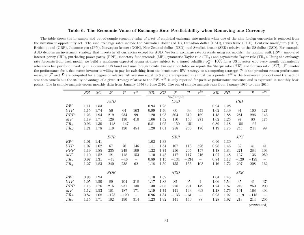
Table 6. The Economic Value of Exchange Rate Predictability when Removing one Currency

The table shows the in-sample and out-of-sample economic value of a set of empirical exchange rate models when one of the nine foreign currencies is removed fromthe investment opportunity set. The nine exchange rates include the Australian dollar (AUD), Canadian dollar (CAD), Swiss franc (CHF), Deutsche mark\euro (EUR),British pound (GBP), Japanese yen (JPY), Norwegian kroner (NOK), New Zealand dollar (NZD), and Swedish kronor (SEK) relative to the US dollar (USD). For example,AUD denotes an investment strategy that invests in all currencies except for AUD. We form exchange rate forecasts using six models: the random walk (RW), uncoveredinterest parity (UIP), purchasing power parity (PPP), monetary fundamentals (MF), symmetric Taylor rule (TR) and asymmetric Taylor rule (TR). Using the exchangerate forecasts from each model, we build a maximum expected return strategy subject to a target volatility ∗= 10% for a US investor who every month dynamicallyrebalances her portfolio investing in a domestic US bond and nine foreign bonds. For each portfolio, we report the Sharpe ratio (SR) and Sortino ratio (SO). F denotesthe performance fee a risk-averse investor is willing to pay for switching from the benchmark RW strategy to a competing strategy. P is the premium return performancemeasure. F and P are computed for a degree of relative risk aversion equal to 6 and are expressed in annual basis points. is the break-even proportional transactioncost that cancels out the utility advantage of a given strategy relative to the RW. is only reported for positive performance measures and is expressed in monthly basispoints. The in-sample analysis covers monthly data from January 1976 to June 2010. The out-of-sample analysis runs from January 1986 to June 2010.

SR SO F P SR SO F P SR SO F P

In-SampleAUD CAD CHF

111 153 094 125 094 128 115 174 56 64 163 099 140 60 69 443 102 149 91 100 127 125 194 219 234 99 120 193 304 319 169 118 188 281 296 146 119 171 128 130 410 106 152 150 153 271 102 125 97 83 175 096 130 −148 −147 − 081 105 −150 −151 − 089 118 −58 −62 − 121 178 119 120 454 120 161 258 253 176 119 175 245 244 99

EUR GBP JPY 101 141 102 133 096 130 107 162 67 76 146 111 154 107 113 526 098 146 32 41 41 119 185 235 249 109 122 174 256 265 157 118 184 271 284 103 110 152 121 118 153 110 145 117 117 216 107 148 137 136 259 097 131 −43 −46 − 089 115 −134 −134 − 084 112 −129 −129 − 127 183 240 238 62 118 159 155 155 103 116 172 207 208 162

NOK NZD SEK 098 124 110 152 104 145 105 150 89 104 218 117 183 85 95 4 106 154 35 41 37 115 176 215 231 130 130 208 278 291 149 124 187 249 259 200 112 153 181 187 171 119 174 141 143 393 118 176 161 168 404 087 108 −123 −120 − 096 134 −133 −131 − 093 127 −119 −118 − 115 171 182 190 314 123 192 141 146 88 128 192 213 214 206

(continued)

31

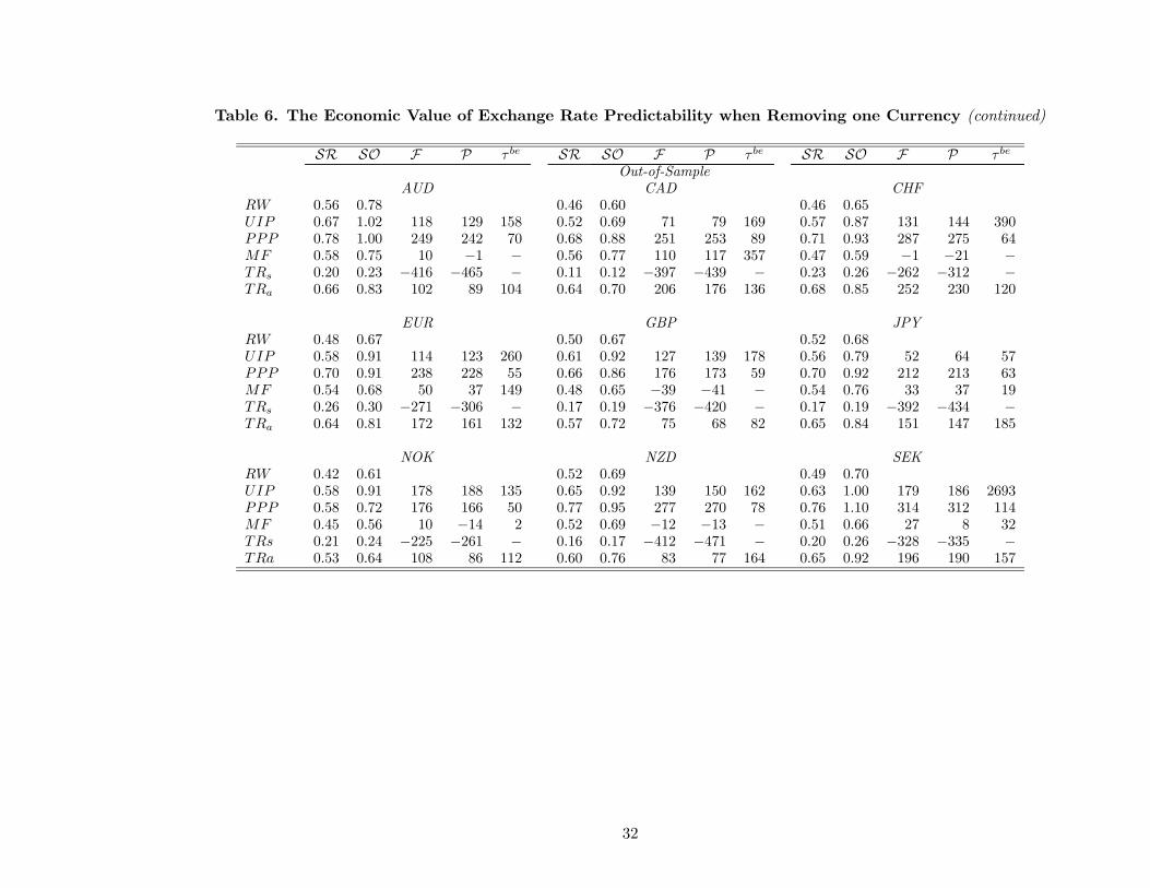
Table 6. The Economic Value of Exchange Rate Predictability when Removing one Currency (continued)

SR SO F P SR SO F P SR SO F P

Out-of-SampleAUD CAD CHF

056 078 046 060 046 065 067 102 118 129 158 052 069 71 79 169 057 087 131 144 390 078 100 249 242 70 068 088 251 253 89 071 093 287 275 64 058 075 10 −1 − 056 077 110 117 357 047 059 −1 −21 − 020 023 −416 −465 − 011 012 −397 −439 − 023 026 −262 −312 − 066 083 102 89 104 064 070 206 176 136 068 085 252 230 120

EUR GBP JPY 048 067 050 067 052 068 058 091 114 123 260 061 092 127 139 178 056 079 52 64 57 070 091 238 228 55 066 086 176 173 59 070 092 212 213 63 054 068 50 37 149 048 065 −39 −41 − 054 076 33 37 19 026 030 −271 −306 − 017 019 −376 −420 − 017 019 −392 −434 − 064 081 172 161 132 057 072 75 68 82 065 084 151 147 185

NOK NZD SEK 042 061 052 069 049 070 058 091 178 188 135 065 092 139 150 162 063 100 179 186 2693 058 072 176 166 50 077 095 277 270 78 076 110 314 312 114 045 056 10 −14 2 052 069 −12 −13 − 051 066 27 8 32 021 024 −225 −261 − 016 017 −412 −471 − 020 026 −328 −335 − 053 064 108 86 112 060 076 83 77 164 065 092 196 190 157

32

Table 7. The Economic Value of Exchange Rate Predictability for Alternative Numeraires

The table presents the in-sample and out-of-sample economic value of a set of empirical exchange rate models for alternative numeraires other than the US dollar. Theset of currencies includes the Australian dollar (AUD), Canadian dollar (CAD), Swiss franc (CHF), Deutsche mark\euro (EUR), British pound (GBP), Japanese yen (JPY),Norwegian kroner (NOK), New Zealand dollar (NZD), Swedish kronor (SEK) and the US dollar (USD). For example, AUD denotes an investment strategy using AUD as thedomestic currency and expressing all exchange rates relative to AUD. We form exchange rate forecasts using six models: the random walk (RW), uncovered interest parity(UIP), purchasing power parity (PPP), monetary fundamentals (MF), symmetric Taylor rule (TR) and asymmetric Taylor rule (TR). Using the exchange rate forecastsfrom each model, we build a maximum expected return strategy subject to a target volatility ∗= 10% for a US investor who every month dynamically rebalances herportfolio investing in a domestic US bond and nine foreign bonds. For each portfolio, we report the Sharpe ratio (SR) and Sortino ratio (SO). F denotes the performancefee a risk-averse investor is willing to pay for switching from the benchmark RW strategy to a competing strategy. P is the premium return performance measure. F and Pare computed for a degree of relative risk aversion equal to 6 and are expressed in annual basis points. is the break-even proportional transaction cost that cancels outthe utility advantage of a given strategy relative to the RW. is only reported for positive performance measures and is expressed in monthly basis points. The in-sampleanalysis covers monthly data from January 1976 to June 2010. The out-of-sample analysis runs from January 1986 to June 2010.

SR SO F P SR SO F P SR SO F P

In-SampleAUD CAD CHF

108 149 108 147 109 144 095 144 −141 −127 − 110 146 55 55 114 128 182 200 207 137 124 194 242 268 54 132 203 306 317 116 141 227 394 412 378 082 129 −285 −269 − 107 186 −11 6 − 104 153 −38 −26 − 106 139 −13 −14 − 093 137 −163 −155 − 102 126 −72 −78 − 149 240 370 373 212 117 164 100 103 316 126 182 190 194 186

EUR GBP JPY 109 144 107 147 109 147 125 174 159 162 170 118 173 133 145 61 116 201 115 140 92 135 198 329 342 245 123 185 222 236 124 138 201 367 375 251 110 167 13 24 8 104 158 −37 −23 − 108 151 11 17 23 107 130 5 1 1 103 147 −50 −49 − 102 142 −86 −80 − 128 182 204 208 290 122 181 157 157 147 124 168 180 183 277

NOK NZD SEK 108 150 107 153 108 150 126 219 146 150 827 105 146 −19 −14 − 100 151 −100 −98 − 124 184 235 248 127 115 185 129 152 28 133 179 340 344 128 131 167 243 239 139 098 162 −114 −107 − 101 158 −62 −46 − 114 157 73 74 8 106 147 −11 −7 − 111 136 45 37 5 133 208 258 265 166 155 261 452 452 401 139 206 292 294 21

(continued)

33

Table 7. The Economic Value of Exchange Rate Predictability for Alternative Numeraires (continued)

SR SO F P SR SO F P SR SO F P

Out-of-SampleAUD CAD CHF

054 075 054 074 054 073 025 036 −333 −326 − 066 088 143 141 169 066 091 134 136 92 054 083 −15 −2 − 066 088 130 131 36 081 118 318 323 103 029 038 −278 −280 − 054 070 20 5 8 028 040 −320 −310 − 042 058 −111 −113 − 024 029 −313 −329 − 033 045 −227 −220 − 046 063 −81 −71 − 060 077 76 57 121 026 033 −333 −349 −

EUR GBP JPY 054 073 053 074 054 073 064 094 113 121 89 064 099 122 137 47 059 094 49 72 23 068 097 155 157 56 051 071 −52 −47 − 086 120 379 381 104 042 051 −145 −183 − 031 043 −250 −244 − 036 053 −191 −184 − 036 043 −235 −259 − 049 072 −38 −34 − 033 041 −222 −225 − 033 039 −254 −284 − 074 102 239 238 102 034 042 −237 −252 −

NOK NZD SEK 053 074 053 075 054 074 050 080 −28 −20 − 045 067 −123 −111 − 052 077 −21 −14 − 065 092 121 126 37 077 103 270 268 45 061 085 70 73 22 060 070 73 49 39 036 042 −173 −207 − 017 023 −471 −476 − 052 077 −3 2 − 029 041 −223 −225 − 047 054 −110 −150 − 067 094 164 163 278 071 093 205 197 109 073 089 217 198 903

34

Table 8. The Economic Value of Combined Forecasts

The table presents the out-of-sample economic value of combined forecasts across a set of empirical exchange ratemodels. We form forecasts for the nine exchange rates using combinations of six models: the random walk (RW),uncovered interest parity (UIP), purchasing power parity (PPP), monetary fundamentals (MF), symmetric Taylor rule(TRs) and asymmetric Taylor rule (TRa). Simple Model Averaging denotes ex-ante combining methods that disregardthe past out-of-sample performance of the individual models and use the mean, median and trimmed mean of theindividual forecasts. Statistical Model Averaging denotes ex-ante combining methods based on the past out-of-samplemean-squared error (MSE) of the individual models. DMSE(θ) use the inverse of the discounted MSE with θ as adiscount factor. MSE(κ) use the inverse of the MSE over the most recent κ months. Economic Model Averagingdenote ex-ante combining methods which use the past out-of-sample Sharpe ratio (SR) of the individual models.DSR(θ) use the discounted SR with θ as a discount factor. SR(κ) uses the average SR over the most recent κmonths. Using the forecast combinations, we build a maximum expected return strategy subject to a target volatilityσ∗p= 10% for a US investor who every month dynamically rebalances her portfolio investing in a domestic US bondand nine foreign bonds. For each portfolio, we report the Sharpe ratio (SR) and Sortino ratio (SO). F denotes theperformance fee a risk-averse investor is willing to pay for switching from the benchmark RW strategy to a competingstrategy. P is the premium return performance measure. F and P are computed for a degree of relative risk aversionequal to 6 and are expressed in annual basis points. τ be is the break-even proportional transaction cost that cancelsout the utility advantage of a given strategy relative to the RW. τ be is only reported for positive performance measuresand is expressed in monthly basis points. The in-sample analysis covers monthly data from January 1976 to June 2010.The out-of-sample analysis runs from January 1986 to June 2010.

µ σ SR SO F P τ be

RW 10.8 11.4 0.54 0.73

Simple Model AveragingMean 13.3 11.6 0.74 0.89 234 206 81

Median 12.0 12.0 0.61 0.74 76 52 21

Trimmed Mean 12.0 12.1 0.60 0.72 65 37 23

Statistical Model AveragingDMSE (θ = 0.90) 13.2 11.7 0.72 0.87 213 186 71

DMSE (θ = 0.95) 13.2 11.7 0.73 0.88 218 191 74

DMSE (θ = 1.00) 13.3 11.6 0.74 0.89 232 204 81

MSE(κ = 60) 13.2 11.7 0.73 0.88 222 195 76

MSE(κ = 36) 13.2 11.7 0.73 0.88 218 191 74

MSE(κ = 12) 13.1 11.7 0.72 0.87 207 179 70

Economic Model AveragingDSR (θ = 0.90) 13.4 11.5 0.76 0.96 254 235 128

DSR (θ = 0.95) 13.4 11.5 0.76 0.95 255 236 127

DSR (θ = 1.00) 12.9 11.4 0.72 0.89 207 187 103

SR(κ = 60) 13.5 11.5 0.76 0.96 261 241 129

SR(κ = 36) 13.4 11.5 0.76 0.95 254 234 126

SR(κ = 12) 13.4 11.5 0.76 0.96 254 235 128

35

Figure 1. Out-of-Sample Sharpe Ratios

The figure displays the out-of-sample annualized Sharpe ratio (SR) for selected empirical exchange rate models. We

show the results from forming exchange rate forecasts using uncovered interest parity (UIP), purchasing power parity

(PPP), asymmetric Taylor rule (TRa), and the ex-ante forecast combination method that uses the out-of-sample SRover the past 60 months (SR(κ = 60)). All models (solid line) are displayed versus the random walk (RW) benchmark

(dashed line). Using the exchange rate forecasts from each model, we build a maximum expected return strategy subject

to a target volatility σ∗p = 10% for a US investor who every month dynamically rebalances her portfolio investing in a

domestic US bond and nine foreign bonds. The SR is computed using the out-of-sample portfolio returns for one year.

The out-of-sample period runs from January 1986 to June 2010.

36

References

Abhyankar, A., L. Sarno, and G. Valente (2005). “Exchange Rates and Fundamentals: Evidence onthe Economic Value of Predictability,”Journal of International Economics 66, 325—348.

Akram, F., D. Rime, and L. Sarno (2008). “Arbitrage in the Foreign Exchange Market: Turning onthe Microscope,”Journal of International Economics 76, 237—253.

Avramov, D. (2002). “Stock Return Predictability and Model Uncertainty,” Journal of FinancialEconomics 64, 423—458.

Bandi, F.M., and J.R. Russell (2006). “Separating Microstructure Noise from Volatility,”Journal ofFinancial Economics 79, 655—692.

Bandi, F.M., J.R. Russell, and Y. Zhu (2008). “Using High-Frequency Data in Dynamic PortfolioChoice,”Econometric Reviews 27, 163—198.

Bates, J.M., and C.W.J. Granger (1969). “The Combination of Forecasts,” Operations ResearchQuarterly 20, 451—468.

Bilson, J.F.O. (1981). “The ‘Speculative Effi ciency’Hypothesis,”Journal of Business 54, 435—451.

Boudoukh, J., M. Richardson, and R.F. Whitelaw (2006). “The Information in Long-Maturity For-ward Rates: Implications for Exchange Rates and the Forward Premium Anomaly,”working paper,New York University.

Brunnermeier, M.K., S. Nagel, and L.H. Pedersen (2009). “Carry Trades and Currency Crashes”NBER Macroeconomics Annual 2008, 313—347.

Burnside, C., M. Eichenbaum, I. Kleshchelski, and S. Rebelo (2011). “Do Peso Problems Explainthe Returns to the Carry Trade?”Review of Financial Studies 24, 853—891.

Campbell, J.Y., and R.J. Shiller (1987). “Cointegration and Tests of Present Value Models,”Journalof Political Economy 95, 1062—1088.

Campbell, J.Y., and R.J. Shiller (1988). “Stock Prices, Earnings, and Expected Dividends.”Journalof Finance 43, 661—676.

Campbell, J.Y., and S.B. Thompson (2008). “Predicting Excess Stock Returns Out of Sample: CanAnything Beat the Historical Average?”Review of Financial Studies 21, 1509—1531.

Cheung, Y.-W., M.D. Chinn, and A.G. Pascual (2005). “Empirical Exchange Rate Models of theNineties: are any Fit to Survive?”Journal of International Money and Finance 24, 1150—1175.

Clarida, R., J. Gali, and M. Gertler (1998). “Monetary Policy Rules in Practice. Some InternationalEvidence,”European Economic Review 42, 1033—1067.

Clarida, R.H., L. Sarno, M.P. Taylor, and G. Valente (2003). “The Out-of-Sample Success of TermStructure Models as Exchange Rate Predictors: A Step Beyond,”Journal of International Economics60, 61—83.

Clarida, R.H., L. Sarno, M.P. Taylor, and G. Valente (2006). “The Role of Asymmetries and RegimeShifts in the Term Structure of Interest Rates,”Journal of Business 79, 1193—1225.

Clark, T.E., and M.W. McCracken (2001). “Tests of Equal Forecast Accuracy and Encompassing forNested Models,”Journal of Econometrics 105, 85—110.

37

Clark, T.E., and M.W. McCracken (2011). “Testing for Unconditional Predictive Ability,”in HendryD., and M. Clements (eds.), Oxford Handbook on Economic Forecasting, Oxford University Press(forthcoming).

Clark, T.E., and K.D. West (2006). “Using Out-of-Sample Mean Squared Prediction Errors to Testthe Martingale Difference Hypothesis,”Journal of Econometrics 135, 155—186.

Clark, T.E., and K.D. West (2007). “Approximately Normal Tests for Equal Predictive Accuracy,”Journal of Econometrics 138, 291—311.

Cremers, M. (2002). “Stock Return Predictability: A Bayesian Model Selection Perspective,”Reviewof Financial Studies 15, 1223—1249.

Della Corte, P., L. Sarno, and G. Sestieri (2010). “The Predictive Information Content of ExternalImbalances for Exchange Rate Returns: How Much Is It Worth?,”Review of Economics and Statistics(forthcoming) doi:10.1162/REST_a_00157.

Della Corte, P., L. Sarno, and D.L. Thornton (2008). “The Expectation Hypothesis of the TermStructure of very Short-Term Rates: Statistical Tests and Economic Value,” Journal of FinancialEconomics 89, 158—174.

Della Corte, P., L. Sarno, and I. Tsiakas (2009). “An Economic Evaluation of Empirical ExchangeRate Models,”Review of Financial Studies 22, 3491—3530.

Della Corte, P., L. Sarno, and I. Tsiakas (2011). “Spot and Forward Volatility in Foreign Exchange,”Journal of Financial Economics 100, 496—513.

Della Corte, P., L. Sarno, and I. Tsiakas (2012). “Volatility and Correlation Timing in Active Cur-rency Management,” in James, J., L. Sarno and I.W. Marsh (eds.) Handbook of Exchange Rates.London: Wiley (forthcoming).

Diebold, F.X., and R.S. Mariano (1995). “Comparing Predictive Accuracy,”Journal of Business andEconomic Statistics 13, 253—263.

Engel, C. (1996). “The Forward Discount Anomaly and the Risk Premium: A Survey of RecentEvidence,”Journal of Empirical Finance 3, 123—192.

Engel, C., N.C. Mark, and K.D. West (2007). “Exchange Rate Models are not as Bad as you Think,”NBER Macroeconomics Annual 2007, 381—441.

Engel, C., and K.D. West (2005). “Exchange Rates and Fundamentals,”Journal of Political Economy113, 485—517.

Evans, M.D.D., and R.K. Lyons (2002). “Order Flow and Exchange Rate Dynamics,” Journal ofPolitical Economy 110, 170—180.

Fama, E.F. (1984). “Forward and Spot Exchange Rates,”Journal of Monetary Economics 14, 319—338.

Fleming, J., C. Kirby, and B. Ostdiek (2001). “The Economic Value of Volatility Timing,”Journalof Finance 56, 329—352.

Goetzmann, W., J. Ingersoll, M. Spiegel, and I. Welch (2007). “Portfolio Performance Manipulationand Manipulation-Proof Performance Measures,”Review of Financial Studies 20, 1503—1546.

38

Gomez, V., and A. Maravall (2000). “Seasonal Adjustment and Signal Extraction in Economic TimeSeries,”in Pena D., G.C. Tiao, and T.R. Tsay (eds.), A Course in Time Series Analysis, New York:Wiley.

Gourinchas, P.-O., and H. Rey (2007). “International Financial Adjustment,” Journal of PoliticalEconomy 115, 665—703.

Goyal, A., and A. Saretto (2009). “Cross-Section of Option Returns and Volatility,” Journal ofFinancial Economics 94, 310—326.

Groen, J.J.J. (2000). “The Monetary Exchange Rate Model as a Long-Run Phenomenon,”Journalof International Economics 52, 299—319.

Hai, W., N.C. Mark, and Y. Wu (1997). “Understanding Spot and Forward Exchange Rate Regres-sions,”Journal of Applied Econometrics 12, 715—734.

Han, Y. (2006). “Asset Allocation with a High Dimensional Latent Factor Stochastic VolatilityModel,”Review of Financial Studies 19, 237—271.

Hodrick, R.J. (1987). The Empirical Evidence on the Effi ciency of Forward and Futures ForeignExchange Markets, London: Harwood.

Hodrick, R.J., and E.C. Prescott (1997). “Postwar U.S. Business Cycles: An Empirical Investigation,”Journal of Money, Credit and Banking 29, 1—16.

Jondeau, E., and M. Rockinger (2008). “Time-Variability in Higher Moments Is Important for AssetAllocation,”Unpublished Working paper, University of Lausanne.

Kilian, L. (1999). “Exchange Rates and Monetary Fundamentals: What do we Learn from Long-Horizon Regressions?”Journal of Applied Econometrics 14, 491—510.

Lothian, J.R., and M.P. Taylor (1996). “Real Exchange Rate Behavior: The Recent Float From thePerspective of the Past Two Centuries,”Journal of Political Economy 104, 488—509.

Mark, N.C. (1995). “Exchange Rates and Fundamentals: Evidence on Long-Horizon Predictability,”American Economic Review 85, 201—218.

Mark, N.C. (2009). “Changing Monetary Policy Rules, Learning, and Real Exchange Rate Dynam-ics,”Journal of Money, Credit and Banking 41, 1047—1070.

Mark, N.C., and D. Sul. (2001). “Nominal Exchange Rates and Monetary Fundamentals: Evidencefrom a Small Post-Bretton Woods Panel,”Journal of International Economics 53, 29—52.

Marquering, W., and M. Verbeek (2004). “The Economic Value of Predicting Stock Index Returnsand Volatility,”Journal of Financial and Quantitative Analysis 39, 407—429.

McCracken, M.W. (2007). “Asymptotics for Out of Sample Tests of Granger Causality,”Journal ofEconometrics 140, 719—752.

Meese, R.A., and K. Rogoff (1983). “Empirical Exchange Rate Models of the Seventies: Do TheyFit Out of Sample?”Journal of International Economics 14, 3—24.

Molodtsova, T., and D.H. Papell (2009). “Out-of-Sample Exchange Rate Predictability with TaylorRule Fundamentals?”Journal of International Economics 77, 167—180.

Neely, C.J., P.A. Weller, and J.M. Ulrich (2009). “The Adaptive Markets Hypothesis: Evidence fromthe Foreign Exchange Market,”Journal of Financial and Quantitative Analysis 44, 467—488.

39

Nelson, C.R., and M.J. Kim (1993). “Predictable Stock Returns: the Role of Small Sample Bias,”Journal of Finance 48, 641—661.

Newey, W.K., and K.D. West (1987). “A Simple, Positive Semi-Definite, Heteroskedasticity andAutocorrelation Consistent Covariance Matrix,”Econometrica 55, 703—708.

Orphanides, A. (2001). “Monetary Policy Rules Based on Real-Time Data,”American EconomicReview 91, 964—985.

Orphanides, A., and S. van Norden (2002). “The Unreliability of Output Gap Estimates in RealTime,”Review of Economics and Statistics 84, 569—583.

Rapach, D.E., J.K. Strauss, and G. Zhou (2010). “Out-of-Sample Equity Premium Prediction: Com-bination Forecasts and Links to the Real Economy.”Review of Financial Studies 23, 821—862.

Rime, D., L. Sarno and E. Sojli (2010). “Exchange Rate Forecasting, Order Flow and MacroeconomicInformation,”Journal of International Economics 80, 72—88.

Rogoff, K.S. (1996). “The Purchasing Power Parity Puzzle,” Journal of Economic Literature 34,647—668.

Rogoff, K.S., and V. Stavrakeva (2008). “The Continuing Puzzle of Short Horizon Exchange RateForecasting,”NBER Working Paper No. 14071.

Sarno, L. (2005). “Towards a Solution to the Puzzles in Exchange Rate Economics: Where Do WeStand?”Canadian Journal of Economics 38, 673—708.

Sarno, L., and E. Sojli (2009). “The Feeble Link Between Exchange Rates and Fundamentals: CanWe Blame the Discount Factor?,”Journal of Money, Credit and Banking 41, 437—442.

Stambaugh, R.F. (1999). “Predictive Regressions,”Journal of Financial Economics 54, 375—421.

Stock, J.H., and M.W. Watson (2003). “Forecasting Output and Inflation: The Role of Asset Prices,”Journal of Economic Literature 41, 788—829.

Stock, J.H., and M.W.Watson (2004). “Combination Forecasts of Output Growth in a Seven-CountryData Set,”Journal of Forecasting 23, 405—430.

Taylor, A.M., and M.P. Taylor (2004). “The Purchasing Power Parity Debate,”Journal of EconomicPerspectives 18, 135—158.

Taylor, J.B. (1993). “Discretion versus Policy Rules in Practice,” Carnegie-Rochester ConferenceSeries on Public Policy 39, 195—214.

Timmermann, A. (2006). “Forecast Combinations,”in Elliott, G., C.W.J. Granger, and A. Timmer-mann (eds.), Handbook of Economic Forecasting, Amsterdam: Elsevier.

Welch, I., and A. Goyal (2008). “A Comprehensive Look at The Empirical Performance of EquityPremium Prediction,”Review of Financial Studies 21, 1455—1508.

West, K.D. (1988). “Dividend Innovations and Stock Price Volatility,”Econometrica 56, 37—61.

West, K.D. (1996). “Asymptotic Inference about Predictive Ability,”Econometrica 64, 1067—1084.

West, K.D. (2006). “Forecast Evaluation,” in: Elliott, G., C.W. Granger, and A. Timmermann,(eds.), Handbook of Economic Forecasting. Vol. 1, Chapter 3, 99—134.

40

West, K.D., H.J. Edison, and D. Cho (1993). “A Utility-Based Comparison of Some Models ofExchange Rate Volatility,”Journal of International Economics 35, 23—45.

Wright, J.H. (2008). “Bayesian Model Averaging and Exchange Rate Forecasting,”Journal of Econo-metrics 146, 329—341.

41