
Statistical Analyses of Surface Temperatures in AR5 · Statistical Analyses of Surface Temperatures...
21
This critique is available at www.informath.org/AR5stat.pdf Statistical Analyses of Surface Temperatures in the IPCC Fifth Assessment Report Douglas J. Keenan 17 December 2013 First version 28 December 2016 This version Acknowledgements: for comments on drafts, I am grateful to Sir David Cox, David Henderson, Demetris Koutsoyiannis, Janice Moore, and William Nordhaus.
Transcript of Statistical Analyses of Surface Temperatures in AR5 · Statistical Analyses of Surface Temperatures...
This critique is available at www.informath.org/AR5stat.pdf
Statistical Analyses of Surface Temperatures
in the IPCC Fifth Assessment Report
Douglas J. Keenan
17 December 2013 First version
28 December 2016 This version
Acknowledgements: for comments on drafts, I am grateful to Sir David Cox, David Henderson, Demetris
Koutsoyiannis, Janice Moore, and William Nordhaus.
1
1. Introduction
In September 2013, the IPCC issued the first volume of its Fifth Assessment Report (AR5). The
volume includes extensive discussions of observations of the average temperature on Earth’s
surface (i.e. where people live). The discussions include some statistical analyses of those
observations. This critique considers the merits of such statistical analyses. No background in
statistics is required.
2. How to do a statistical analysis
To understand statistical analysis, consider an example. Suppose that we toss two coins, and
we ask what the probability is that both coins come up heads. To determine the probability,
we will make two reasonable assumptions: (i) the probability that a coin comes up heads is ½
and (ii) one toss has no effect on the other toss. Then, the probability of two heads is
calculated to be ½ × ½ = ¼.
In general, any statistical analysis will consist of two phases. The first phase is to make some
assumptions about the process that generates the data (in our example, we made two such
assumptions). The second phase is to do some mathematical calculations (in our example, we
did a simple multiplication).
The assumptions are obviously vital for the analysis. If, for instance, we had assumed that the
probability a coin comes up heads is 1/3, then our final answer would have been different: 1/9.
The assumptions, collectively, are called the “statistical model”. Every statistical analysis thus
vitally depends on what statistical model—i.e. set of assumptions—is chosen.
Although the mathematical calculation in our example was simple, it can sometimes be very
complicated. Such complication used to be a major difficulty for statistical analyses (and if you
studied statistics in the 20th century, you would have spent much effort considering how to do
such complicated calculations). Nowadays, though, there is usually an easy way.
To illustrate the easy way, consider our example of tossing two coins. Instead of calculating
the probability of getting two heads, we could estimate the probability as follows: take two
coins, toss them a million times, and count the number of times that both coins come up
heads. I tried doing that, and counted 249943 times that both coins came up heads; thus the
estimated probability is 249943/1000000, which is not exactly ¼, but is extremely close. The
lack of exactness will almost always be negligible, in practice.
2
I did not actually toss coins a million times, of course. Rather, I used a computer program to
roughly simulate doing that. The program was based on the two assumptions that we made.
In other words, what I actually did was use a program that simulated the statistical model.
This method of running a program that simulates the model a large number of times can often
be used, instead of doing the mathematical calculation. The method is called the “Monte
Carlo method”. The method has been known for decades, but techniques for applying it
quickly and accurately were first developed only around the year 2000. (The algorithm that
led to this development is the Mersenne Twister.)
The development of the Monte Carlo method implies that the second phase of a statistical
analysis can often be done almost mechanically. Nowadays, then, it is often the first phase—
selecting an appropriate model—that is the sole difficult task in statistical analyses.
3. Significant trends
Imagine tossing a coin ten times. If the coin came up Heads each time, we would have very
good evidence that the coin was not a fair coin. Suppose instead that the coin was tossed only
three times. If the coin came up Heads each time, we would not have good evidence that the
coin was unfair: getting Heads three times can reasonably occur just by chance.
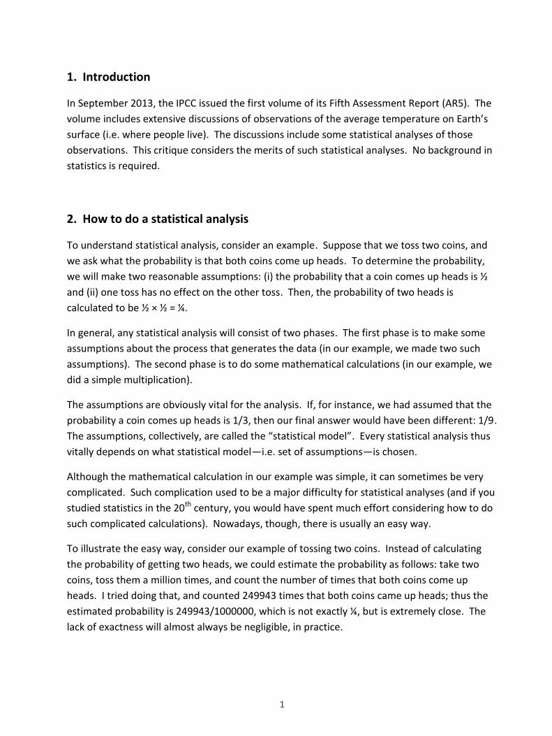
In Figure 1, each graph has three segments, one segment for each toss of a coin. If the coin
came up Heads, then the segment slopes upward; if it came up Tails, then the segment slopes
downward. In Figure 1, the graph on the left illustrates tossing Heads, Tails, Heads; the middle
graph illustrates Tails, Heads, Tails; and the last graph illustrates Heads, Tails, Tails.
Figure 1. Coin tosses: H, T, H (left);
T, H, T (middle); H, T, T (right).
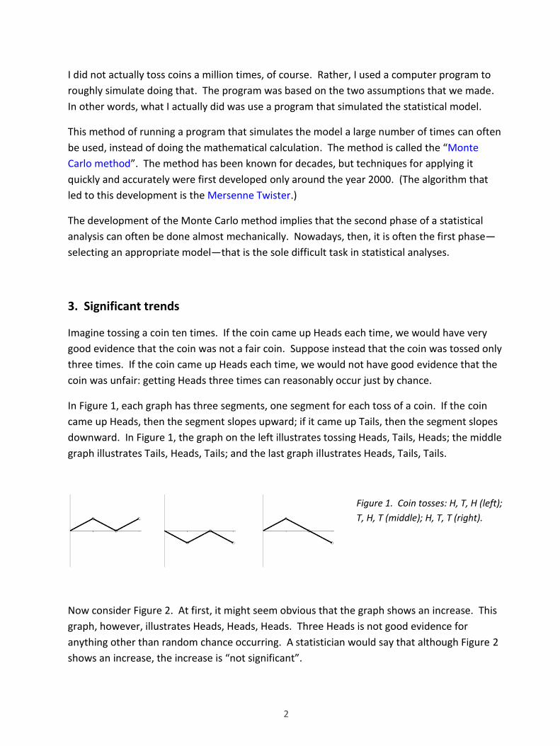
Now consider Figure 2. At first, it might seem obvious that the graph shows an increase. This
graph, however, illustrates Heads, Heads, Heads. Three Heads is not good evidence for
anything other than random chance occurring. A statistician would say that although Figure 2
shows an increase, the increase is “not significant”.
3
Figure 2. Coin tosses: H, H, H.
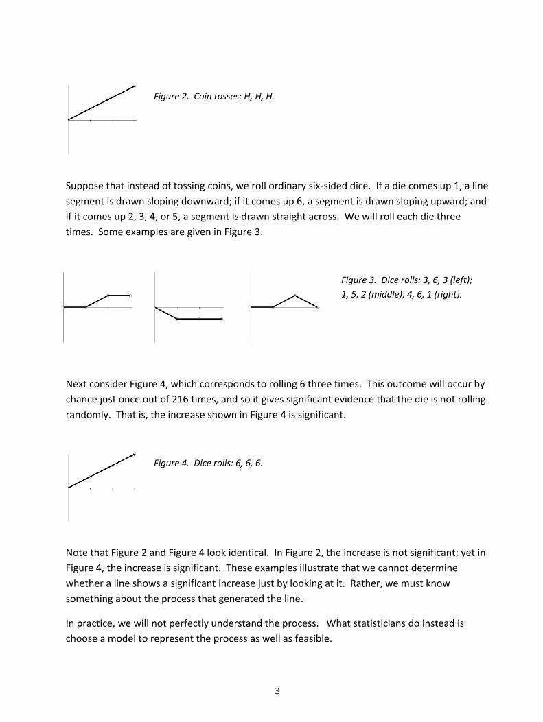
Suppose that instead of tossing coins, we roll ordinary six-sided dice. If a die comes up 1, a line
segment is drawn sloping downward; if it comes up 6, a segment is drawn sloping upward; and
if it comes up 2, 3, 4, or 5, a segment is drawn straight across. We will roll each die three
times. Some examples are given in Figure 3.
Figure 3. Dice rolls: 3, 6, 3 (left);
1, 5, 2 (middle); 4, 6, 1 (right).
Next consider Figure 4, which corresponds to rolling 6 three times. This outcome will occur by
chance just once out of 216 times, and so it gives significant evidence that the die is not rolling
randomly. That is, the increase shown in Figure 4 is significant.
Figure 4. Dice rolls: 6, 6, 6.
Note that Figure 2 and Figure 4 look identical. In Figure 2, the increase is not significant; yet in
Figure 4, the increase is significant. These examples illustrate that we cannot determine
whether a line shows a significant increase just by looking at it. Rather, we must know
something about the process that generated the line.
In practice, we will not perfectly understand the process. What statisticians do instead is
choose a model to represent the process as well as feasible.
4
An increase that is significant under one model might well be insignificant under another
model, as illustrated. Put plainly, we can reach almost any conclusion, by (mis)choosing a
suitable model. Again, the choice of model is vital.
4. Time series
A concept from statistics that we need is that of a time series. A time series is any series of
measurements taken at regular time intervals. Examples include the following: prices on the
New York Stock Exchange at the close of each business day; the maximum temperature in
London each day; the total wheat harvest in Canada each year. Another example is the
average global temperature each year.
Suppose that today is extremely warm, at some location. Then there is a tendency for
tomorrow to be warmer than average. More generally, what happens at some time in the
future can be dependent upon what is happening now. Note that this is different from what
happened when we tossed two coins: with the two coins, the outcome of the second toss was
not dependent upon the outcome of the first toss.
Having future events be dependent upon the present complicates the statistical analysis of
time series. Some elaboration on that is given in Excursus 1.
Excursus 1. As a first example, consider how the temperature today is correlated
with the temperature tomorrow. The statistical analysis of daily temperatures
should consider that correlation. Next, consider how the temperature during the
past week will have some correlation with the temperature tomorrow. Again, the
statistical analysis should consider that. Then consider how the temperature
during the present season will tend to have some correlation with the temperature
tomorrow. More generally, many different time scales are potentially relevant, and
those time scales should be considered. Furthermore, the various correlations
need not be linear. Properly accounting for all these issues is problematic.
The complications arising in the analysis of time series tend to make the selection of a
statistical model for a time series difficult. Indeed, one of the world’s leading specialists in
time series, Howell Tong, stated the following, in his book Non-linear Time Series (§5.4).
A fundamental difficulty in statistical analysis is the choice of an appropriate model.
This is particularly pronounced in time series analysis.
5
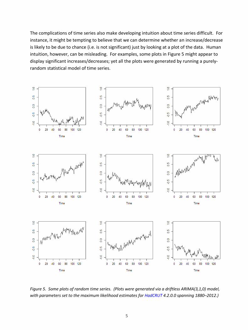
The complications of time series also make developing intuition about time series difficult. For
instance, it might be tempting to believe that we can determine whether an increase/decrease
is likely to be due to chance (i.e. is not significant) just by looking at a plot of the data. Human
intuition, however, can be misleading. For examples, some plots in Figure 5 might appear to
display significant increases/decreases; yet all the plots were generated by running a purely-
random statistical model of time series.
Figure 5. Some plots of random time series. (Plots were generated via a driftless ARIMA(3,1,0) model,
with parameters set to the maximum likelihood estimates for HadCRUT 4.2.0.0 spanning 1880–2012.)
6
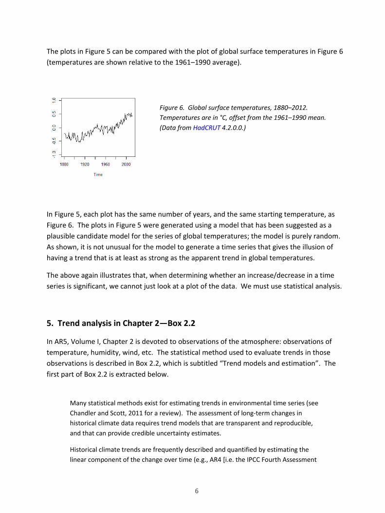
The plots in Figure 5 can be compared with the plot of global surface temperatures in Figure 6
(temperatures are shown relative to the 1961–1990 average).
Figure 6. Global surface temperatures, 1880–2012.
Temperatures are in °C, offset from the 1961–1990 mean.
(Data from HadCRUT 4.2.0.0.)
In Figure 5, each plot has the same number of years, and the same starting temperature, as
Figure 6. The plots in Figure 5 were generated using a model that has been suggested as a
plausible candidate model for the series of global temperatures; the model is purely random.
As shown, it is not unusual for the model to generate a time series that gives the illusion of
having a trend that is at least as strong as the apparent trend in global temperatures.
The above again illustrates that, when determining whether an increase/decrease in a time
series is significant, we cannot just look at a plot of the data. We must use statistical analysis.
5. Trend analysis in Chapter 2—Box 2.2
In AR5, Volume I, Chapter 2 is devoted to observations of the atmosphere: observations of
temperature, humidity, wind, etc. The statistical method used to evaluate trends in those
observations is described in Box 2.2, which is subtitled “Trend models and estimation”. The
first part of Box 2.2 is extracted below.
Many statistical methods exist for estimating trends in environmental time series (see
Chandler and Scott, 2011 for a review). The assessment of long-term changes in
historical climate data requires trend models that are transparent and reproducible,
and that can provide credible uncertainty estimates.
Historical climate trends are frequently described and quantified by estimating the
linear component of the change over time (e.g., AR4 [i.e. the IPCC Fourth Assessment
7
Report]). Such linear trend modelling has broad acceptance and understanding based
on its frequent and widespread use in the published research assessed in this report,
and its strengths and weaknesses are well known (von Storch and Zwiers, 1999; Wilks,
2006). Challenges exist in assessing the uncertainty in the trend and its dependence on
the assumptions about the sampling distribution (Gaussian or otherwise), uncertainty
in the data used, dependency models for the residuals about the trend line, and
treating their serial correlation (Von Storch, 1999; Santer et al., 2008).
The quantification and visualisation of temporal changes are assessed in this chapter
using a linear trend model that allows for first order autocorrelation in the residuals
(Santer et al., 2008; Supplementary Material 2.SM.3). Trend slopes in such a model are
the same as ordinary least squares trends; uncertainties are computed using an
approximate method. The 90% confidence interval quoted is solely that arising from
sampling uncertainty in estimating the trend.
There is no a priori physical reason why the long-term trend in climate should be linear
in time. Climatic time series often have trends for which a straight line is not a good
approximation (e.g., Seidel and Lanzante, 2004). The residuals from a linear fit in time
often do not follow a simple autoregressive or moving average process, and linear
trend estimates can easily change when estimates are recalculated using data covering
shorter or longer time periods or when new data are added. When linear trends for
two parts of a longer time series are calculated separately, the trends calculated for
two shorter periods may be very different (even in sign) from the trend in the full
period, if the time series exhibits significant nonlinear behavior in time (Box 2.2,
Table 1).
The first paragraph is reasonable. The reference by Chandler and Scott is a book, which
contains a section entitled “The linear trend” (§3.1); this section correctly states that “it is
necessary to check the assumptions of any model before interpreting the results”. In other
words, if the model’s assumptions have not been argued to be valid, then we cannot use the
model to draw any inferences about the data.
The second paragraph correctly states that “Challenges exist in assessing the uncertainty in the
trend”—and thus, in particular, assessing whether the trend is significant.
The third paragraph states that the IPCC has chosen a statistical model that comprises a
straight line with first-order autocorrelated noise. If you are unfamiliar with such noise, that
does not matter here. What is important here is that a model has been chosen, yet there is no
scientific justification given for the choice. The failure to present any evidence or logic to
support the assumptions of the model is a serious violation of basic scientific principles.
8
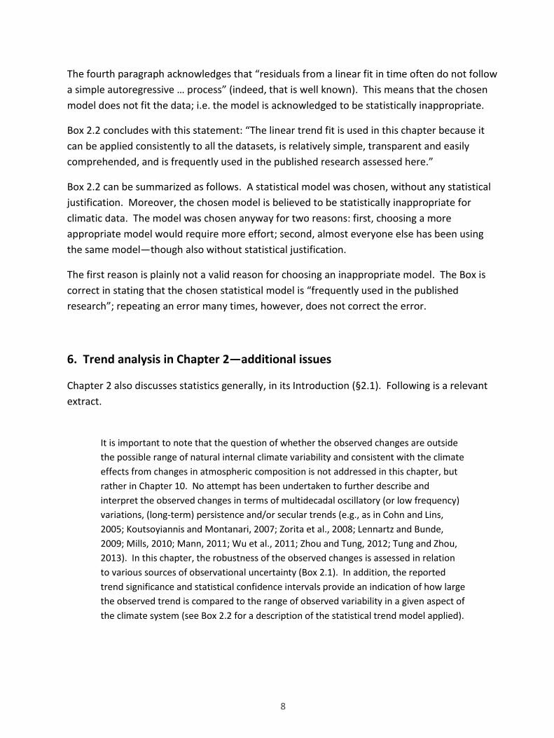
The fourth paragraph acknowledges that “residuals from a linear fit in time often do not follow
a simple autoregressive … process” (indeed, that is well known). This means that the chosen
model does not fit the data; i.e. the model is acknowledged to be statistically inappropriate.
Box 2.2 concludes with this statement: “The linear trend fit is used in this chapter because it
can be applied consistently to all the datasets, is relatively simple, transparent and easily
comprehended, and is frequently used in the published research assessed here.”
Box 2.2 can be summarized as follows. A statistical model was chosen, without any statistical
justification. Moreover, the chosen model is believed to be statistically inappropriate for
climatic data. The model was chosen anyway for two reasons: first, choosing a more
appropriate model would require more effort; second, almost everyone else has been using
the same model—though also without statistical justification.
The first reason is plainly not a valid reason for choosing an inappropriate model. The Box is
correct in stating that the chosen statistical model is “frequently used in the published
research”; repeating an error many times, however, does not correct the error.
6. Trend analysis in Chapter 2—additional issues
Chapter 2 also discusses statistics generally, in its Introduction (§2.1). Following is a relevant
extract.
It is important to note that the question of whether the observed changes are outside
the possible range of natural internal climate variability and consistent with the climate
effects from changes in atmospheric composition is not addressed in this chapter, but
rather in Chapter 10. No attempt has been undertaken to further describe and
interpret the observed changes in terms of multidecadal oscillatory (or low frequency)
variations, (long-term) persistence and/or secular trends (e.g., as in Cohn and Lins,
2005; Koutsoyiannis and Montanari, 2007; Zorita et al., 2008; Lennartz and Bunde,
2009; Mills, 2010; Mann, 2011; Wu et al., 2011; Zhou and Tung, 2012; Tung and Zhou,
2013). In this chapter, the robustness of the observed changes is assessed in relation
to various sources of observational uncertainty (Box 2.1). In addition, the reported
trend significance and statistical confidence intervals provide an indication of how large
the observed trend is compared to the range of observed variability in a given aspect of
the climate system (see Box 2.2 for a description of the statistical trend model applied).

9
This claim is key: “the question of whether the observed changes are outside the possible
range of natural … climate variability … is not addressed in this chapter”. This chapter, though,
does contain statistical analyses. The above text additionally claims that the purpose of those
analyses is to “provide an indication of how large the observed trend is compared to the range
of observed variability”.
In other words, the statistical analyses do not indicate whether the observed increases are
outside the range of natural variability, but they do indicate if the observed increases are large
compared to the range of variability. Obviously, the two claims conflict with each other.
Additionally, the term “observed trend” is misleading, because trends are generally meaningful
only with confidence intervals (or similar). Confidence intervals, though, are not observed;
rather, they are derived via the statistical model (which is chosen via human judgement).
Furthermore, by acknowledging that “No attempt has been undertaken to further describe
and interpret the observed changes in terms of multidecadal oscillatory (or low frequency)
variations, (long-term) persistence and/or secular trends …”, Chapter 2 is (again) effectively
acknowledging that there are statistical models that might well be more appropriate than the
model that was chosen. And the chapter is deliberately avoiding considering those models.
The stated reason for not considering those models is that the purpose of the chapter is to
consider “observational uncertainty”. For an example of observational uncertainty, we can
examine the global surface temperature in 2012. The best estimate of that temperature is
0.45 °C (relative to the 1961–1990 average temperature). The value 0.45 °C, though, is not
exact, because we do not have exact temperature measurements for every place in the world.
Researchers, however, have stated that they are 90% confident that the exact temperature
was in the interval 0.37–0.53 °C. That interval, known as a “90%-confidence interval”, is a way
of indicating what the uncertainty is in the estimate of the 2012 temperature.
Chapter 2 is supposed to present observations of surface temperatures, and other aspects of
the atmosphere, and to indicate how much uncertainty there is in each of those observations.
Chapter 2 actually discusses uncertainty only a little.
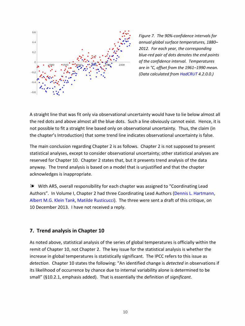
Some illustration of the uncertainty for global temperatures is given in Figure 7. For the last
year shown in the figure, 2012, there are two dots: one blue, at 0.37 °C; one red, at 0.53 °C.
Thus, the dots indicate the 90%-confidence interval for the temperature in 2012. The other
dots indicate similarly for the other years.
10
Figure 7. The 90%-confidence intervals for
annual global surface temperatures, 1880–
2012. For each year, the corresponding
blue-red pair of dots denotes the end points
of the confidence interval. Temperatures
are in °C, offset from the 1961–1990 mean.
(Data calculated from HadCRUT 4.2.0.0.)
A straight line that was fit only via observational uncertainty would have to lie below almost all
the red dots and above almost all the blue dots. Such a line obviously cannot exist. Hence, it is
not possible to fit a straight line based only on observational uncertainty. Thus, the claim (in
the chapter’s Introduction) that some trend line indicates observational uncertainty is false.
The main conclusion regarding Chapter 2 is as follows. Chapter 2 is not supposed to present
statistical analyses, except to consider observational uncertainty; other statistical analyses are
reserved for Chapter 10. Chapter 2 states that, but it presents trend analysis of the data
anyway. The trend analysis is based on a model that is unjustified and that the chapter
acknowledges is inappropriate.
❧ With AR5, overall responsibility for each chapter was assigned to “Coordinating Lead
Authors”. In Volume I, Chapter 2 had three Coordinating Lead Authors (Dennis L. Hartmann,
Albert M.G. Klein Tank, Matilde Rusticucci). The three were sent a draft of this critique, on
10 December 2013. I have not received a reply.
7. Trend analysis in Chapter 10
As noted above, statistical analysis of the series of global temperatures is officially within the
remit of Chapter 10, not Chapter 2. The key issue for the statistical analysis is whether the
increase in global temperatures is statistically significant. The IPCC refers to this issue as
detection. Chapter 10 states the following: “An identified change is detected in observations if
its likelihood of occurrence by chance due to internal variability alone is determined to be
small” (§10.2.1, emphasis added). That is essentially the definition of significant.
11
The relevant section of Chapter 10 is §10.2.2, entitled “Time-series methods, causality and
separating signal from noise”. The section begins by comparing the statistical analysis of data
to the analysis that is done via supercomputer simulations of the global climate system. It
states this: “The advantage of [time-series] approaches is that they do not depend on the
accuracy of any complex global climate model, but they nevertheless have to assume some
kind of model, or restricted class of models …”. This statement is correct—and crucial.
The section also includes the following statements.
Time-series methods ultimately depend on the … adequacy of the statistical model
employed.
The assumptions of the statistical model employed can also influence results.
All these [time-series] approaches are subject to the issue of confounding factors….
Again, all of this is correct. In stating these things, the section is presenting the basics of the
statistical situation reasonably fairly.
Additionally, §10.2.2 states this: “Trends that appear significant when tested against [the
statistical model used in Chapter 2] may not be significant when tested against [some other
statistical models]”. Thus, §10.2.2 effectively acknowledges that the statistical model used in
Chapter 2 should not have been relied on.
So, what statistical model does §10.2.2 choose? None. That is, §10.2.2 effectively
acknowledges that we do not understand the data well enough to choose a statistical model.
It does that even though it also acknowledges that choosing such a model is required for
drawing inferences. The conclusion is thus clear: it is currently not possible to draw inferences
from the series of global temperatures. This conclusion is extremely important. It should have
been stated explicitly, and it should have been noted in the Executive Summary of Chapter 10.
Although this critique is focused on surface temperature observations, the same statistical
criticism applies to other claims of observational evidence for significant global warming.
Simply put, no one has yet presented valid statistical analysis of any observational data to
show global warming is real. Moreover, that applies to any warming—whether attributable to
humans or to external natural factors, such as the sun. This is implied by §10.2.2, and indeed it
is clear from the statistics.
12
8. Summary for Policymakers
The most important part of AR5 is arguably the Summary for Policymakers (SPM) in Volume I.
The SPM synopsizes all the chapters in the volume, and it is intended to directly influence
national governments.
The first section of the SPM, after the introduction, lists bullets points of evidence for global
warming. The first bullet point thus appears as the single most important piece of evidence for
global warming, from the perspective of policymakers. The first bullet point begins as follows.
The globally averaged combined land and ocean surface temperature data as
calculated by a linear trend, show a warming of 0.85 [0.65 to 1.06] °C, over the period
1880 to 2012….
(The numbers in square brackets indicate the 90%-confidence interval. Having the confidence
interval so far away from including 0 implies that the trend is extremely significant.)
The claim in the bullet point is essentially copied from the Executive Summary of Chapter 2,
which claims that “global combined land and ocean surface temperature data show an
increase of about 0.85 [0.65 to 1.06] over 1880–2012 … when described by a linear trend”.
The claim, however, is untenable, as discussed above and as acknowledged by §10.2.2.
Simply put, the SPM ignores what is said in Chapter 10. It does that even though responsibility
for the statistical analysis lies with Chapter 10.
9. Trend analysis by the Met Office
The statistical model used in Chapter 2 of AR5, Volume I, was also used in Fourth Assessment
Report (AR4), published in 2007. As a result of being used in AR4, the model has been studied
by, amongst others, the Met Office, which is the primary institute for global-warming research
in the UK. (The Met Office was originally known as the “Meteorological Office”.)
A research paper studying the statistical model used in Chapter 2 was published by the Met
Office Chief Scientist, Julia Slingo, in May 2013. The paper is entitled “Statistical models and
the global temperature record”. It effectively acknowledges that the statistical model of
Chapter 2 is untenable for the series of global temperatures. Moreover, although it considers
other models, it does not attempt to select a model for the series. In short, the paper comes
to essentially the same conclusion as §10.2.2.
13
The events that led to the writing of the paper are noteworthy. Briefly, Lord Donoughue
submitted a Parliamentary Question that asked if the rise in global temperatures since 1880
was statistically significant. The Answer, which was sourced from the Met Office, was yes. The
statistical model upon which the answer was based, however, was the statistical model used in
AR4 (and Chapter 2 of AR5). Hence, I contacted Lord Donoughue, explained that the Answer
was untenable, and offered my services as a statistical adviser.
Lord Donoughue then submitted another Parliamentary Question, which essentially asked if
the statistical model used for the prior Question was justified. The Met Office refused to
answer the Question. Lord Donoughue asked again, and again—five times in total—and he
was refused each time.
The rules of Parliament require Parliamentary Questions to be answered. Lord Donoughue,
though, was unsure about how to enforce that; indeed, he would later remark, “In 28 years in
Parliament I do not recall such obfuscation”. In consequence, Lord Donoughue consulted with
the Leader of the House of Lords and the Deputy Clerk of the Parliaments. He then sent a
letter to the responsible minister, the Parliamentary Under Secretary of State for Energy and
Climate Change.
The minister, Baroness Verma, had previously been signing off on answers obtained from the
Met Office, on the assumption that the Met Office was acting in good faith. Upon receipt of
the letter, the minister required the Met Office to answer the question properly. The proper
answer was then given in Parliament: the statistical model is untenable. Moreover, the Met
Office told Parliament that it did “not use a linear trend model to detect changes in global
mean temperature”. The paper written by the Chief Scientist, cited above, is essentially an
elaboration on that.
For more details on the foregoing events, see the Bishop Hill blog post entitled “Met Office
admits claims of significant temperature rise untenable”. Simply put, the Met Office, in
particular its Chief Scientist, was attempting to mislead Parliament.
There have been other situations where Chief Scientist Slingo made statistical claims about the
climate that she knew were highly misleading. An example is described in the Bishop Hill blog
post “Climate correspondents”.
In AR5, Volume I, the SPM relies upon the same statistical model as the IPCC had used in AR4—
as discussed above. Hence, I sent the following message to Chief Scientist Slingo.
The IPCC’s AR5 WGI Summary for Policymakers includes the following statement.

14
The globally averaged combined land and ocean surface temperature data as calculated by a linear trend, show a warming of 0.85 [0.65 to 1.06] °C, over the period 1880–2012….
(The numbers in brackets indicate 90%-confidence intervals.) The statement is near the beginning of the first section after the Introduction; as such, it is especially prominent. The confidence intervals are derived from a statistical model that comprises a straight line with AR(1) noise. As per your paper “Statistical models and the global temperature record” (May 2013), that statistical model is insupportable, and the confidence intervals should be much wider—perhaps even wide enough to include 0 °C. It would seem to be an important part of the duty of the Chief Scientist of the Met Office to publicly inform UK policymakers that the statement is untenable and the truth is less alarming. I ask if you will be fulfilling that duty, and if not, why not.
I did not receive a reply. In an attempt to get an answer, Lord Donoughue has now submitted
some further Parliamentary Questions.
10. The crucial question
The crucial question is this: what statistical model should be chosen? Both the IPCC (§10.2.2)
and the Met Office have considered that question; neither found an answer. Indeed, finding
an answer would require some original research.
The central issue here is simple, and does not require training in statistics to understand. The
central issue is this: if assumptions are made in a scientific analysis, then those assumptions
should not be merely proclaimed, but rather given some scientific justification. Yet, virtually
all statistical analyses of climatic data proceed by merely proclaiming some assumptions.
The full situation is even worse, because the assumptions that are commonly used in statistical
analyses of climatic data are not only unjustified, but also unjustifiable; i.e. it is known that the
assumptions are inappropriate for the data. An example of that is in AR5, Volume I: the
statistical analysis in the chapter on atmospheric observations (Chapter 2) relies on an
assumption that is known to be inappropriate. Astoundingly, the inappropriateness is
acknowledged in the chapter, as well as in another chapter which has the responsibility for the
statistical analysis (Chapter 10).
There seems to be only one scientist who has seriously attempted to answer the crucial
question, i.e. to choose a statistical model. That scientist is Demetris Koutsoyiannis, at the

15
National Technical University of Athens. Koutsoyiannis has not (yet) found a viable answer to
the question; at least, though, he has tried to. No other researcher has tried, to my
knowledge. For an introduction to some of the work of Koutsoyiannis, see Excursus 2.
Excursus 2. The number of statistical models that could potentially be considered
for the global temperature series is infinite. How can we choose among those
models? A leading statistician in the U.S. said the following, in an e-mail to me.
My sense is that the observed time series is not sufficiently long
to cleanly distinguish among various time series models, nor to
definitively demonstrate man-made warming versus natural cycles
versus (for some models) a mostly flat trend.
Indeed, that should be obvious to anyone who has reasonable skill at the analysis
of time series. It is only true, however, if we are considering purely-statistical
analyses. Generally, though, analyses of data should incorporate some knowledge
of the application area: in this case, the physics of the climate system. That is, we
should try to use physics to constrain the set of candidate models. That strategy
has also been suggested by a statistician at the Met Office, Doug McNeall.
Although that strategy is clear and arguably necessary, implementing it seems to be
extremely difficult. The only researcher who has attempted implementing it, as far
as I know, is Koutsoyiannis. Koutsoyiannis invokes thermodynamic constraints, in
particular. For a non-technical overview of his approach, see the Bishop Hill blog
post “Koutsoyiannis 2011”.
The reliance on merely proclaimed assumptions, in statistical analyses of climatic data, implies
that virtually all claims to have drawn statistical inferences from climatic data are untenable.
In particular, there is no demonstrated observational evidence for significant global warming.
11. Conversations with some British climate scientists
I had an e-mail discussion with a Senior Scientist at the Met Office about the existence of
evidence for global warming. The scientist, Vicky Pope, had published an article about global
warming in The Guardian (on 23 March 2012). The article claimed that “[global warming] is a
matter of science and therefore of evidence – and there’s lots of it”, that a “whole range of
different datasets and independent analyses show the world is warming”, and that there is
16
“overwhelming evidence for man-made climate change”. The article, however, did not
substantiate those claims.
Hence, I e-mailed Pope, saying “I ask you to detail a single piece of observational evidence, and
supporting analysis, for global warming”. Pope replied politely, but her reply did not specify
any evidence. I answered, inter alia, “I note that your message does not present any piece of
observational evidence, despite my asking for one piece”. Pope again replied politely, but
again her reply did not specify any evidence; rather, her reply said “I will think about how and
where to respond to the particular points that you raise”.
Thus, it seems that a Senior Scientist at the Met Office is aware that there is no demonstrated
observational evidence for (significant) global warming. As noted earlier, it also seems that the
Chief Scientist at the Met Office is aware. And now, with AR5, there seems to be awareness in
Volume I, §10.2.2.
You might well ask how the misperception that observational evidence exists could have
become widespread. Part of the problem is that climatologists generally have no training in
the statistical analysis of time series—even though almost all climatic data sets are time series.
In other words, climatologists do not know how to statistically analyse climatic data.
An exemplification of this occurred at a debate related to global warming that was held in July
2010. The debate was hosted by The Guardian. There were five panellists, including a former
chair of the IPCC, Bob Watson, and myself. Another one of the panellists was a Pro Vice
Chancellor from the University of East Anglia, Trevor Davies; Davies oversees the work done at
the university’s Climatic Research Unit (CRU), which is the most prominent institution for
global-warming research in the UK after the Met Office; he was previously a researcher at CRU.
The current head of research at CRU is Phil Jones, who is considered by many people to be the
most eminent climatologist in the UK. Jones’ specialty is analysing climatic data. From my
reading of some of Jones’ research publications, though, I concluded that Jones has negligible
competence at data analysis. For that reason, I stated the following, during the debate.
I think people are really overestimating the competence and the skill of some of these
scientists. Phil Jones, for example, could absolutely not pass an examination in an
introductory undergraduate course in statistical time series.
After the debate, Davies told me that Jones could pass such an examination. I then offered to
pay £500/minute to have Jones write the examination. My offer was not accepted. Thus,
Davies seemed to implicitly admit that one of the world’s leading specialists in analysing
climatic data did not have any competence at statistically analysing such data.
17
Jones, though, should not be singled out for criticism here. A lack of competence with time-
series is exhibited by almost all climatologists (including those sceptical about global warming).
There have been some attempts to persuade climatologists to consider statistical analysis of
time series more carefully, by both myself and others. Such attempts are almost always
rebuffed. It is easy to criticize climatologists for that; before doing so, though, it is worth
attempting to put yourself in their place.
Imagine that you had earned a Ph.D. in climatology: that takes about five years of hard work,
on very tiny pay. Then you worked hard for decades more, earned respect from your peers,
and essentially founded your professional identity on being an expert in the study of the
climate system. And now, someone comes along and tells you that most of the work you and
your colleagues have done during your careers is invalid, due to a statistical problem. How
would you respond? Would you say, “Oh, that’s nice—thanks for letting me know”?
Scientists are human, and they respond in human ways. One key to understanding what has
happened with climate science is to consider not just the science, but also the scientists.
12. The Australian experience
The Australian government commissioned a study on the impacts of global warming on the
Australian economy. The study was led by a distinguished professor of economics in Australia,
Ross Garnaut, and it is known as the “Garnaut Review”. The Review began by assessing the
scientific basis for global warming. That assessment concluded that global warming is a
serious threat to the world.
Garnaut conducted the assessment of the scientific basis as follows. First, he recognized that
almost all climatic data sets are time series, and thus analysing climatic data requires doing
time-series analysis. Second, he commissioned two time-series specialists in Australia to
analyse the series of global surface temperatures. Third, he founded the Review, in part, on
the results of that analysis. In short, the scientific foundation of the Review was conducted in
an exemplary way.
The statistical analysis that served as the foundation of the Garnaut Review is detailed in a
paper, “Global temperature trends”, written by the two time-series specialists—Trevor
Breusch and Farshid Vahid. I found invalidating errors in that analysis. I e-mailed Breusch and
Vahid about the errors in June 2011. Breusch replied politely, but seemed to not understand
the issues. I responded, elaborating and giving references. There were no further e-mails.
18
The statistical errors are actually clear and basic. A slightly oversimplified description of the
errors is given in Excursus 3.
Excursus 3. When choosing a statistical model, one of the methods used by
statisticians is to employ what is called “relative likelihood”. Using this method, we
can tell that one model is, e.g., 1000 times more likely than another model to be
the better model of the data (where “better” is defined in a certain technical way).
If one model is 1000 times more likely than another, second, model, then we would
conclude that the second model should be rejected. If the first model is only a few
times more likely than the second model, though, then we should not reject the
second model. The situation here is analogous to gambling: if the odds are 1000 to
1 in our favour, then we are almost certain to win (in the analogy, be choosing the
better model); if the odds are only 3 to 1 in our favour, then we might well lose (in
the analogy, be choosing the worse model).
Breusch & Vahid considered some statistical models for the temperature series.
The models that they considered, though, were all linear. Excluding nonlinear
models is questionable. Indeed, the IPCC has previously noted that “we are dealing
with a coupled non-linear chaotic system” (AR3, Volume I, §14.2.2.2).
Having restricted their consideration to only linear models, Breusch & Vahid then
chose a model for which the increase in global temperatures is significant. Yet
there were other models that were nearly as likely as the chosen model: thus, the
choice of Breusch & Vahid was ill founded.
With some of the other models that were nearly as likely as the chosen model, the
increase in temperatures is not significant. To summarize—some likely model
shows the increase as significant and other likely models show the increase as not
significant. Hence, we cannot determine whether the increase is significant. The
main conclusion of Breusch & Vahid, however—based on their choice of model—is
that the increase is significant. The main conclusion is thus actually baseless.
It is notable that the Met Office Chief Scientist, in her paper cited above,
considered some linear models very similar to those considered by Breusch &
Vahid. The Chief Scientist reasoned that the likelihood comparisons were
“inconclusive”; so she did not choose among the models. She did find that the
most likely model was one for which the increase in temperatures is significant.
She noted, however, that there were other models that were nearly as likely and
for which the increase is not significant. Hence, she drew no inferences regarding
significance. In other words, when in essentially the same situation as Breusch &

19
Vahid, the Chief Scientist reached the correct conclusion. (This conclusion is also
effectively implied by the more general considerations of AR5, Volume I, §10.2.2.)
❧ Breusch and Vahid were sent a draft of this critique, on 27 October 2013. I have not
received a reply.
13. An example from outside climatology
Vital problems with statistical analyses exist in fields of research other than global-warming
science. An example from another field is described here. The field is tephrochronology,
which studies the chemistry of volcanic ash.
In statistics, there is a concept known as “standard error”; the concept is taught in all
introductory statistics courses. A substantial portion of modern tephrochronology, though, is
substantially based on misinterpreting the concept. The misinterpretation has sometimes led
to conclusions that are the opposite of what would be concluded if the correct interpretation
were used. I published a paper on this, in 2003. My paper was published in the leading journal
for geochemistry, but it has since been largely ignored.
Not all fields of science do statistical analyses incompetently though. One branch of science
where gross statistical incompetence occurs only rarely is medical science. Up until this
century, however, statistical analyses in medical science were often appalling. A statistician at
Oxford University, Doug Altman, campaigned against incompetent statistics in medical
research. His campaign included publishing works such as “The scandal of poor medical
research” and “Poor-quality medical research”. After about a decade of this, the International
Committee of Medical Journal Editors agreed to a major change in the way research
manuscripts are peer reviewed: the Committee’s Uniform Requirements for Manuscripts was
changed to include strong requirements for statistical methods. Moreover, if a manuscript
relies on non-trivial statistics, medical journal editors now commonly call in a statistician as an
extra reviewer. Since the change, statistical analyses in medical science have dramatically
improved (though they are still far from perfect).
The foregoing illustrates that vital problems with statistical analyses exist, or have existed, in
scientific fields other than climatology. Such problems can be at the level of an introductory
statistics course, as in tephrochronology. Such problems can have enormous consequences, as
in medicine. And rectification of such problems can be fought against by almost all scientists in
the relevant field, as in both tephrochronology and medicine. Any attempt to understand the
source of the problems in global-warming science should consider that.

20
Appendix. Foundations of statistics
The main foundation of climatology is agreed upon by all climatologists: it comprises Newtonian
mechanics, classical chemistry, etc. The main foundation of statistics, though, is not agreed upon
by statisticians: rather, there are different contenders for the foundation. One of those
contenders is called frequentism. The frequentist foundation inherently leads to using significance
levels, confidence intervals, etc.; it is the best known foundation among climatologists, by far.
Because frequentist statistics is so well known among climatologists, it has been generally adopted
in this critique. The issues raised in this critique, though, are not dependent upon the foundation:
all the issues can be recast for other foundations (in particular, for the Bayesian foundation and for
the information-theoretic foundation).
_________________________________________ _________________________________________
The reason for so much bad science is not that talent is rare, not at all; what is rare is character. People are not honest, they don’t admit their ignorance, and that is why they write such nonsense.
—Sigmund Freud
Half the harm that is done in this world is due to people who want to feel important. They don’t mean to do harm—but the harm does not interest them. Or they do not see it, or they justify it because they are absorbed in the endless struggle to think well of themselves.
—T.S. Eliot
You should, in science, believe logic and arguments, carefully drawn, and not authorities.
—Richard P. Feynman


