Stationary and quasi-stationary eddies in the extratropical troposphere

-6-

Stationary and quasi-stationary eddies in the extratropical

troposphere: theory ISAAC M. HELD

6.1. Introduction

The climatological zonal asymmetries in the atmosphere result from asymmetries in the Earth's surface. The problem of explaining the atmospheric asymmetries is complicated by the fact that some of the relevant surface properties, such as ocean temperature, land-surface albedo and ground wetness, are at least partially conteolled by the atmosphere. Yet, even if one ignores these important feedback processes and simply prescribed boundary conditions, the construction of a theory explaining the atmospheric asymmetries remains a difficult challenge. This is particularly so for the asymmetries within the troposphere, where latent heat release and the mixing of momentum and heat by large-scale transients are both dependent on the boundary conditions and the forced wave structure in ways that are little understood.

There exist several recent reviews of problems associated with stationary eddies on various scales, most notably Smith (1979) and Dickinson (1980) on the effects of orography. The intention in this survey is not to present a systematic review of theory but simply to touch upon some of the theoretical issues that have arisen time and again since the pioneering work of Charney and Eliassen (1949), Bolin (1950) and Smagorinsky (1953) on planetary-scale stationary waves. Among these issues are the following:

1. What is the relative importance of topographic forcing and zonally asymmetric diabatic heating in determining the planetary stationary wave structure?

128 I. M. HELD

2. To what extent can the observed low-frequency variability in the atmosphere be associated with anomalous fo rced waves?

. 3. Wby do barotropic models of topographically forced waves work as well as they do?

4. Are forced stationary waves potentially resonant?

Two additional questions concerning Rossby wave propagation arise naturally in discussions of 3 and 4:

S. Are stationary Rossby waves absorbed or reflected when they encounter low latitude easterlies?

6. Tn what sense, if any, does the tropopause act as if it were a rigid lid ?

Without at least partial answers to basic questions such as these, one is not in a very good position to address the problems mentioned in the opening paragraph, concerning the various and subtle ways in which the stationary eddies interact with laten t heat release, large-scale transients and the underlying surface.

We begin by describing the response to orography in three linear models: a barotropic model on a beta-plane channel; a barotropic model on a sphere; and a baroclinic, quasi-geostrophic model on a beta-plane channel. These models illustrate the zonal, meridional and vertical propagation of Rossby waves and raise questions 3- 6 in relatively simple settings. The emphasis in these sections is on orographic forcing, not because thermal forcing is unimportant (it is not), but partly because the actual diabatic heating distribution in the troposphere is poorly known, and partly because the problem of thermal forci ng is complicated by the dependence of the response on the vertical as well as horizontal structure of the forcing. The linear response to diabatic heating is then briefly discussed in Section 6.S.

Following this review oflinear forced wave theory, results from atmospheric general circulation models (GeMs) of relevance for questions 1 and 2 are discussed. A comparison of GeMs with realistic orography and with a flat lower boundary is used to address 1, whereas statistics from a GeM with zonally symmetric lower boundary conditions and, therefore, a zonally symmetric climate are used to attempt to shed some light on 2.

The discussion throughout is restricted somewhat arbitrarily to the · problem of explaining the stationary and quasi-stationary eddies in the extratropical Northern Hemisphere troposphere during winter. However, many of the ideas are relevant to the summer season and to the Southern Hemisphere.

j

THEORY OF STATIONARY EDDIES 129

6.2 Barotropic model in a beta-plane channel: zonal propagation of Rossby waves

The classic paper by Charney and Eliassen (1949) contains the first attempt at quantitative modelling of planetary-scale stationary waves. Using a barotropic model on a beta-plane, linearized about a uniform westerly zonal wind flowing over surface topography, these authors obtained a striking fit to the wintertime 500 mb stationary geopotential field along 4SON. It is worthwhile discussing this calculation in detail both because of its historical importanee and because it raises the issue of the potential for r~sonant behaviour of stationary waves in a very simple context.

Postponing any attempt at justification, consider the equation for conservation of potential vorticity for the hydrostatic, depth-independent flow of a homogeneous layer of fluid with a free surface:

(6.1)

H = h - hT, where H is the layer thickness, h the height of the free surface and hT the height of the rigid lower boundary. The notation is otherwise conventional. In the quasi-geostrophic approximation on a beta-plane, (6.1) reduces to:

(:t + vgv)q =0, (6.2)

where q = fo + fJy + ( - fo(ry - hT)/ho, ho is the mean depth, ry = h - ho, v, = g/ fokx Vry and ( = (g/ fO)V2ry (compare with the general formulation in the Appendix-Eqns. AlO and All). Linearizing about a zonal flow [u] = - (glfo) o[ ry]/oy independent of x, y and t and retaining only the lowest-order tenu in the topographic forcing, one obtains for the perturbation (denoted by a *)

(~ + [u] .'l.)q* + u* o[q] = 0, ot ox oy

(6.3a)

where q* = (* - fO<ry* - hT)/ho and o[q]/iJy = fJ + [U]/}.2 with}.2 = gho/f{ Substituting for q* and a[ q]/ay an alternative form of this equation is:

From (6.3a) and (6.3b), the dispersion relation for free plane waves, ry* = Re fi exp i(kx + Iy - wt), is

130 I. M. HELD

(j) = +U] - a~;]/(k2 + [2 + ,1. - 2)} (6.4a)

= k{[u](k2 + 12) _ P}/(k' + (2 + ,1.- 2). (6.4b)

(Note that (j) is not equal to the frequency ofa Rossby wave in the absence of mean flow, Doppler shifted by kii. As is clear from (6.4a), a 'non-Doppler' effect results from the mean flow being balanced by a height gradient that alters 8[q]/oy. As discussed by White (1977), precisely the. same eITect occurs in a continuously strati ned flow, where it enters through the lower boundary condition and has caused some confusion in the literature.) If [u] < 0 the system cannot support a stationary Rossby wave, whereas if ["] > 0 the total wavenumber of the stationary wave is k2 + {2 ,. K 2 = P/["] ,. K;. This stationary wavenumber is independent of ,1.. If one is only interested in the stationary flow, and if the flow is quasi-geostrophic, there is no advantage in the use of the divergent rather than non-divergent vorticity equation.

Consider the steady version of Eqn. (6.3) in a channel geometry, assuming that ~. and hr are both proportional to sin (Iy). Fourier analysing in x and denoting Fourier amplitudes by tildes, one finds that:

(6.5)

For K > K, (K < K ,), the response is exactly in (out of) phase with the topography, with the topographic source of vorticity balanced primarily by the zonal (meridional) advection of relative (planetary) vorticity. Following Charney and Eliassen, the resonance singularity is removed by adding Ekman pumping, which amounts to adding a linear damping on the vorticity in this barotropic model. For steady flow, Eqn. (6.3b) is modified to:

a(* [ u ]fo ahT [ll] - + pv* = -r(* - ----, Ox ho ax

(6.6)

resulting in the modified Fourier amplitudes:

(6.7)

with s ,. rK 2/k[u]. Charney and Eliassen justify this barotropic model by starting with the

quasi-geostrophic vorticity equation and assuming that the flow is separable, '1 = A (x, y)B(z); tbe choice of vertical structure B(z) is then based on observations. As described in the Appendix, [u] on the lhs of Eqn. (6.6) is reinterpreted as a mid-tropospheric wind, whereas [11] on the rhs is reinterpreted as a surface wind- and then replaced byO.4[u], so that the implied vertical velocities are of reasonable magnitude. A more satisfying procedure for justifying barotropic calculations is discussed in Section 6.4.

The variance ortbe solution to (6.6), ['1*2);is plotted in Fig. 6.1 as a function

o w

'" 'l , o '" w o i:? 3

2 " «

3

4

o 10


2

" I \ 20 DAYS I \

I \ " \ ; \0 DAYS

I '. r5 0AYS

/ "i/'

20

V (m s- I)

, ,

25 30

Fig. 6.1. The mean square height response, ['1*2], in the Charney- Eliassen model as a function of [u] fo'r different strengths of dissipation. in units of 104 m2 , The integers

mark the values of [u] at which particular zonal wavenumbers resonate.

of [u] for different values of r, The x-dependence of hrused is obtained from the smoothed topography at 45°N in the GCM discussed in Section 6.6, and is plotted in Fig. 6.2. The meridional wavenumber is chosen so that one halfwavelength equals 35° latitude, while Jo = 20 sin (45°) and ho = 8Ian. The results show a clear resonance structure when ' r - I = 20 days, with the wavenumber 2 resonance dominant but with 3, 4 and 5 also apparent. Little of this structure remains at r - t = 5 days.

Figurc6.2comparcsthesolution~*(x)forr - 1 = 5daysand[u] = 17ms- 1

with the climatological 500 mb height at 45° for January. (As in Charney and Eliassen, [u] on the rhs of Eqn. (6.6) has been multiplied by 0.4.) Since thermal forcing contributes a substantial part of this mid-tropospheric eddy field (see Section 6.6), one should consider the excellence ofthis fit as accidental. It is still of interest, however, that responses of the correct order of magnitude and structure are obtained for values of r sufficiently large that the system does not resonate.

To explore this point further, the total response has been split into two parts in Fig. 6.3, that due to the topography of the Eastern Hemisphere and that due to the topography of the Western Hemisphere. The total response is clearly the sum of two well-defined wavetrains, one emanating from the Rockies and the other, somewhat stronger, from the Tibetan Plateau, Each of the wavetrains decays eastward sufficiently rapidly that there is only modest interference between the two. For this large a dissipation, it is evidently more fruitful to

132 J. M. HELD

200

100

~ 0

t;; '" '" or

-100

- 200

0 90E 180 90W o 2 km

1 km

lONGITUDE

Fig. 6.2. Upper figure : the height response as a function of longitude in the Charney- Eliassen model for the parameters listed in the text (solid line), and the observed climatological 500 mb eddy heights at 45°N in January, from Oort (1982)

(dashed line). Lower figure: the topography h,.{x ) used in Ihe calculation.

200 - - - EASTERN tlEMISPHERE --- -- - WESTERN HEMISPHERE

100

:§: , , ..... /. -... ~ , , .... 0 :J: ,

'" .... ~ - --OJ :J:

-100

- 200

o 90E 180 90W o Fig. 6.3. The response shown in Fig. 6.2 split into the parts due to the topography of

the western and eastern hemispheres.


think in terms of wave trains emanating from localized features, that is, Green's fUDctions, rather than Fourier components.

The solution to Eqn. (6.6) on a channel of infinite length can be written, for sufficiently small ,., in the form:

~'(x, y) = sin (Iy) J:oo G(x - x')h.,(x' ) dx', (6.8)

where:

G(x - x') = 0 if x ,;; x',

= - k ~ 2 sin (k,(x - x')) exp [ - r(x - x')je<J , ifx~xJ.

k, = (K; - 12)' /2 is assumed real, and ex is the zonal group velocity for nondiverllent Rossby waves evaluated at the stationary wavenumber:

(6.9)

ex is always positive and less than 2[ u J. It is because ex is positive that the response is confined to the east of the source. As long as the width of the mountain is much less than the stationary wavelength, and as long as the wave is damped out before progressing around the latitude circle and returning to the source region, the response will resemble tbis Green's function. There will be anticyclonic vorticity over the mountain and a trough immediately downstream, with the stationary wavenumber clearly apparent in the response.

In this simple model, the parameter r determines whether or not the picture of the wave field as composed of potentially resonant Fourier components or of damped wavetrains is the most appropriate. The choice ,. - 1 = 5 days, for which the latter picture seems more appropriate, is rather small for a spindown time due to surface friction, but tbere are otber potential sources of dissipation in the troposphere, most notably mixing due to large-scale transients. More importantly, waves can also disperse into low latitudes and into the stratosphere, from which they may be lmable to return to the region of forcing. We return to this problem in the following sections.

Tbe character of the long-period variability of the forced waves sbould be markedly different depending on whether or not the waves are potentially resonant. If they are potentially resonant, one expects these low-frequency anomalies to be of global scale. One also expects dramatic variations in amplitude and phase, with 180" phase reversals in individual zonal wavenumbers as the flow passes through resonance. In such circumstances, zonal Fourier analysis is clearly illuminating. In contrast, in the non-resonant dissipative or dispersive case one expects anomalies to be local, unless the

134 I. M. HELD

o [uJ

G

[u, ] [uJ

Fig. 6.4. A schematic of the graphic solution for the equilibrium states in the Charney-DeVore modeL

mean flow variations happen to be coherent around a latitude circle, and one does not expect Fourier decomposition to provide the simplest picture of the wave field. A simple shift in the wavelength downstream of the Rockies, say, could be disguised as a complex redistribution among several Fourier components.

Resonant behaviour can have more subtle consequences for variability in the atmosphere, as is evident in the intriguing recent work of Charney and Devore (1979) (see also Charney et al., 1981) on the possible importance of wave-mean flow interaction for the maintenance of anomalous forced wave patterns. In the presence of dissipation the steady forced waves generated by topography exert a drag on the zonal flow, !»([ u ]). Following Charney and Devore, suppose that in the absence of this drag the mean flow relaxes to some [u,] > 0, i.e. :

8~~] ~ -1C([U] - [u,]) - !»([u]). (6.10)

!»([ u]) is the sum of the eddy momentum flux divergence and the form drag, or 'mountain torque',

8 1 !»([ u]) ~ - [u*v*] + - [pO 8hT/8x]

8y ho

~ -[V*I*] - fa [v*hT]

ho

~ -[v*q*]

where p* is the perturbation pressure and q* is the perturbation potentiat


vorticity. If the wave consists of only one meridional mode, sill (Iy), one can show that:

r!o'K'lhTI' sin' (Iy) !liI([ u]) = 2[ u ]h~«K' _ K;)' + E'l"

Thus, !liI([u]) has basically the same shape as [~"] ill Fig. 6.l.

(6.11)

A graphical solution to the steady-state equation, !liI([II]) = ,,([u,] - [II]) is shown in Fig. 6.4. (For the purposes of this qualitative argument, we ignore the y-variation in !liI([u]).) If the parameters are such as to produce the graph shown, three possihle equilibria exist, labelled A, Band C in the figure. It is intuitively clear from Eqn. (6.10) that if" + d!lil/d[ u] is negative, as it is for B, the state is unstable. The high-index, small-wave amplitude state C is associated by these authors with the 'normal' flow, and the low-index, amplified-wave state A with 'blocking'. Without the resonant structure in !liI([u]), multiple equilibrium states of this sort do not occur.

6.3 Barotropic model on a sphere: meridional propagation of Rossby waves

6.3.1 Numerical results

These results for barotropic flow in a beta-plane channel are substantially modified when account is taken of the spherical geometry and mean flow variation with latitude> as recently described by Grose and Hoskins (1979). Although these authors study a divergent shallow water model, the free surface has· no effect on quasi-geostrophic stationary waves, as described in Section 6.2, and we therefore restrict the following discussion to the spherical version of Eqn. (6.6):

[u] . a( + v'(~ am + p) = - [u,]! ahT _ r(' (6.12) a cos q, a" a aq, hoa cos q, a"

with

( 1 al/! 1 01/1)

(II, v) =0 -a aq,' a cos q, 0" .

The coefficient r is taken to be independent of latitude. We describe responses to this equation with hT equal to the Northern

Hemisphere topography used in the GeM described in Section 6.6 and with hT = 0 in the Southern Hemisphere. The topography is shown in Fig. 6.5. [II] and [u,] are set equal to the zonally averaged 300 mb and surface winds produced by the 'no-mountain' model in Section 6.6, and are shown in Fig. 6.6, The choice of300 mb winds is guided by the experience of Grose and Hoskins, who

136 1. M. HELD

160 .' -~ - - . --""

~ . '.

'\ v ,

" " .. , ,", .-... ~

---. -. - --.~ . . - .. : .. -o

·e.

,.'

QI '\),'

-~:,.~

/,/ '0

Fig. 6.5. The topography used in the spherical barotropic calculations, taken from the low resolution spectral model described in Section 6.6. The contour interval is 500 m and heights over 1 km are shaded. The zero contour is not shown. The concentric

dotted circles are 200 latitude apart, the outer circle being the equator.

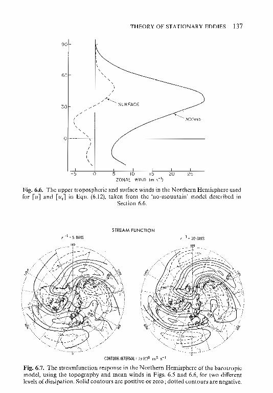
find that this choice produces realistic wave patterns. The model's [u] is everywhere positive, so problems associated with 'critical latitudes' (latitudes at which [u] = 0) do not arise, The streamfunctions obtained by solving Eqn, (6,12) for two values of ,. - 1, 5 days and 20 days, are shown in Fig, 6,7, The corresponding height fields, computed from the approximation q = iiP/g," are shown in Fig, 6,8, Several aspects of these responses are worth noting:

L The height field response is everywhere less than 60 m, The amplitude at 45°N is more than a factor of three smaller than that obtained with the Charney-Eliassen model, using the identical topography along 45°, Roughly half of this difference in amplitude can be explained by setting "Tin the spherical model equal to h,(45°) sin (ly) in the latitude band correspond- . iog to the domain of the Charney-Eliassen model, with lIT == 0 outside of this band and with I andtu.] asin that model. The rest of the difference must be due to the two-dimensional rather than the one-dimensional dispersion of Rossby waves away from localized sources. This particular barotropic model on a sphere, at least, seriously underestimates the amplitude of the orographically forced waves in the mid-troposphere (see Section 6.6),.


90

60

300mb

5 10 15 20 25 ZONAL WIND (m 5- 1)

Fig. 6.6. The upper tropospheric and surface winds in the Northern Hemisphere used for [1I] and [usJ in Ego, (6.12), taken from the 'no-mountain' model described in

Section 6.6.

STREAM FUNCTION (-1=5 DAYS r-1=200AYS

CONTOUR INTERVAL' I x 106 m2 5- 1

Fig. 6.7. The streamfunction response in the Northern Hemisphere of the barotropic model, using the topography and mean winds in Figs. 6.5 and 6.6, for two different levels of dissipation. Solid contours are positive or zero; dotted contours are negative.

138 I. M. HELD

GEOPOTENTlAl

r-I "20 OArs

CONTOUR IN1EHVAl.' 10m

Fig. 6.8. As in Fig. 6.7, but for the height response,N /g.

However, comparison with Fig. 2.2 shows the very realistic nature of the pattern obtained.

2. The amplitudes of the dominant troughs downstream of the Tibetan Plateau and the Rockies are nearly identical for the two values ofr shown. The perturbations further downstream are naturally more sensitive to the level of dissipation, as is evident in the streamfunction maps in which one can follow the equatorward propagating wavetrains into the tropics. This contrasts sharply with the channel model, in which the amplitude of the entire response is sensitive to the value of r in this range, as is dear from Fig. 6.1.

3. As pointed out by Grose and Hoskins, the geopotential response gives the misleading impression of predominantly zonal propagation because of the factor f oc sin </> multiplying the streamfunction. In contrast, the streamfunction responses seem to be dominated by two wavetrains propagating southeastwards, one produced by the Rockies and the other by the Tibetan plateau. Besides these two dominant groups, there are other highs and lows that are with more difficulty associated into wavetrains. The separate · responses to the topography of the Eastern and Western Hemispheres are plotted in Fig. 6.9 using r- 1 ~ 20 days. The interference between these two parts of the response is modest: the Tibetan plateau response decreases the strength of the low in eastern North America hy 15%, whereas the response to the Rockies has almost no effect on the low on the east Asian coast. (This result should be sensitive to the structure of the zonal flow, howevec.) Ina.

THEORV OF STATIONARV EDDIES 139

EASTERN WESTERN

Fig. 6.9. The streamfunction response of Fig. 6.7 with r - 1 = 20 days, split into the responses to the topography of the Eastern and Western Hemispheres.

channel model with the same value of r, interference between the Rocky and Tibetan responses is much more substantial, due to the meridional confinement of the waves.

6.3.2 Meridional dispersion

As noted by Hoskins and Karoly (1981), Rossby wave ray tracing theory explains these structures rather well. For this purpose it is advantageous to transform the linearized un(orced inviscid vorticity equation into Mercator coordinates;

so that:

dq, dy x = a..t; =

cos q,' a

A iJ (0' 0') _ _ _ 0",u Ox ax' + oy2 '" - -p Ox

where u '" [u ]/cos q, and P '" cos q,(P + l/a a[(]/aq,). For a wave of the form "" = Re if exp (ikx), one has

a'if = (k' - Plu)if. ay'

(6.13)

(6.14)

Given a source localized in lati tude, zonal wavenumbers k > k, '" (Plli)l!' are meridionally trapped in the vicinity of the source, while wavenumbers k < k,

140 1. M. HELD

90

60

~

'" ~ l= :5 TRAPPED

30

PROPAGATING

TRAPPED o~ __ ~ __ ~ __ ~ __ ~ __ ~~ o 2 4 6 8 10

ZONAL WAVENUMBER

Fig.6.10. The wavenumber, I1s = aks, dividing propagating from evanescent solutions for a mean wind resembling the wintertime flow at 300 mb, from Karoly (1978). The arrows indicate the potential for meridional confinement of wavenumber 3 near 55°,

propagate away from the source. Fig. 6.10 taken from Karoly (1978), shows n, = ak, as a function of latitude for a particular wintertime_300 mb zonally averaged wind. 11, -> rL) near lOON, where [u] = O. In the easterlies south of this latitude, all waves are trapped.

A source localized in longitude as well as latitude can be thought of as producing two rays for each 11 < 11" corresponding to the two possible meridional wavenumbers, at = ± (n; - n2 )'/2. Since the meridional group velocity of non-divergent Rossby waves, c, = ow/ol = 2Pkt(k 2 + 12

) - 2, has the same sign as I, the positive (negative) sign corresponds to poleward (equatorward) propagation. The rays can be traced downstream in the usual way: the zonal wavenumber characterizing the wave group remains unchanged because the mean flow is independen t of x, whereas the meridional wavenumber adjusts to satisfy the local dispersion relation; the ray path is tangent to the vector group velocity (cx , c,) at this k and t. The amplitude of the streamfunction envelope is proportional to 1- 1i2. One can show further that ray paths are always refracted toward larger 'refractive index' (1l; - n2)1 /2, i.e., towards larger n" this result being equivalent to Snell's law in optics. At a 'furning latitude', where n = 11" one finds that 1-> 0, c,-> 0 and an incident poleward propagating wavetrain is simply reflected and continues propagating eastward. At a critical latitude, where [u] = 0, t-> rL) but c,-> O once again. Rays are refracted into the large region near the critical latitude. In fact,

I' I'

l I:


ex/e, -> 0 as 1-> 00, so the rays approaching the critical latitude are oriented north- south. Examples of ray path calculations can be found in Hoskins and Karoly (1981). For zonal flows with uniform angular rotation the rays are great circles. In other cases this is qualitatively true away from critical lat itudcs, in good agreement with the observations described in Chapter 3.

It is possible for rays to be trapped away from the critical latitude; for example, the ray corresponding to n ~ 3 in Fig. 6.10 is just barely trapped in the high Ii, region near 55°. However, waves can be ex pected to tunnel through the small region of low n, near 45° and continue propagating into the tropics, so this flow will not provide a very efficient cavity for capturing an Ii = 3 resonance. The form of n,(y) is sensitive to the curvature of [u] , and using climatological wintertime 300 mb winds in Oort (1982), one does not find a well-defined dip in Ii, in mid-latitudes. On the other hand, one suspects that substantial changes in curvature occur at particular times, creating more imposing barriers to equatorward propagation, with modest changes in [Il] itself. Meridional trapping of this kind is a distinct possibility and may be of importance for the variability of forced waves in the atmosphere. In its absence, however, all rays are eventually attracted into the zero-wind line. The possibility of resonance behaviour then depends on whether or not the complex dynamics in the vicinity of the zero-wind line results in significant reflection of the incident waves.

6.3.3 The critical latitude

If y, is this criticallatitude and if Du/Dy of 0 at y = y" then I ex: (y - yol - I/' and e, ex: (y - y,)3/' as y -> Yo' One is tempted to conclude that the packet will never reach Ye. since JY C; 1 ~ 00 as y ---+ YC' However, this is not the case, since this 'WKB' theory breaks down: WKB predicts that streamfunction amplitude is proportional to 1- 1/' ex: (y - yJ' /' , so that (iJ'A/iJr)/A ex: (y _ y,)- ', which eventually 'grows larger than /2 ex: (y - yJ- I as y -> y" implying substantial fractional changes in amplitude over one wavelength. With the very small meridional scales generated as y, is approached, one expects nonlinearity or dissipation of some sort to come into play.

By adding a linear damping -1'(, to the vorticity equation and then taking the limit of vanishing 1', one obtains the familiar result that such a linear dissipative critical layer absorbs incident Rossby waves, at least partially. An indication of this behaviour can be gained without obtaining lhe explicit solution. Consider tbe simplest problem ofa'inean flow with II = "l > 0 for y > Y l and u = U2 < 0 for Y < Y2. where (4 1 and U2 are constants, with a wave incident on the zero-wind line between YI illld Y2 from tbe north. F rom the vorticity equation:

r = iPiJ/(kfi - ir),

142 I. M . HELD

one has :

[v" '] = _-_Plv_12 Im(., _ 1--,-. --'-l)' 2" " - u·k

(6.1S)

But:

lim 1m ~ = 10 ."/0 I ~(y - y,), 1: ---0 U - ,e u y

where ~ is the Dirac delta-function. Since [v>(>] = - (%y)[ u'v'] , ["'v>] must be constant with latitude in the limit /' --> 0, except for a jump at the critical latitude:

• • • * nPlvl --, I [u v JI,>" =[u v ]11'<1', + 2kI0"/oyl )'~Y, (6.16)

In the constant Ii easterly region, if oc exp (/ , y), so tbat [u*v*] = 0, whereas in the constant Ii westerly region the solution has the form of an incident wave (with amplitude normalized to unity) plus a reflected wave, if oc exp ( - illY) + R exp (il,y), so tbat

[ * *]1 kl, 2 nPlVl' I u v PI', =2 (1 - IRI ) = 2klou/oyl y ~y: (6.17)

Assuming that fJ > 0 and Iiii' f 0 at y" we must have IRI' < L Part of tbe incident wave has been absorbed, decelerating the mean flow in the process. The amount of absorption is dependent on lVI', and its determination generally requires an explicit solution. Dickinson (1968) shows that the absorption is complete if the region in which WKB is valid overlaps with the region around the critical latitude within which Na can be replaced by y(y - y,) - l, with ya constant.

Tbe physical relevance of this absorbing critical layer has been questioned in light of the work of Benney and Bergeron (1969) on the possibility of a nonlinear balance in tbe critical layer. For a discussion of this theory in an atmospheric context, see Tung (1979). Benney and Bergeron's solution matches asymptotically to a linear solution far from the critical layer, consisting of incident and rellected waves of equal magnitudes. Simplified wave-mean flow calculations (Geisler and Dickinson, 1974) suggest one way of understanding these rellections: the waves modify the mean flow in the vicinity of y, in such as way as to drive fJ close to zero; Eqn. (6.17) then implies that IRI = I. The realizability of a strongly reflecting critical layer remains a problem of fundamental importance for stationary wave theory:

If the equatorward propagating waves are organized into localized wave trains, several additional problems arise concerning the critical latitude. The nonlinear critical layer solution matches onto incident plus reflected waves of a single zonal wavenumber. It is not clear tbat tbe behaviour of an ~


?

90'

LONGITUO[

Fig. 6.11. Schematic of the Rossby wavetrain generated by the Tibetan plateau propagating into the tropics.

incident packet localized in longitude can be inferred from this solution or if nonlinearity results in significant coupling of dilferent zonal wavenumbers. Also, the two dominant wavetrains in Fig. 6.9 enter the tropics in the central Pacific and in the Atlantic and should, therefore, be more sensitive to the structure orthe zonal wind in these regions than to the zonal mean of the zonal wind. The areas of easterlyzorial flow at 200 mb in the time mean January flow taken from Newell et al. (1974) are indicated by the shaded areas in Fig. 6.1l. The regions of westerlies in the equatorial western Pacific and the Atlantic suggest the possibility that these wavetrains partially avoid zero-wind lines. This idea is returned to in Section 9.5.l.

Some of the low-frequency variability in the extra tropical height field is known from the work of Horel and Wallace (1981) and others to be correlated with equatorial Pacific sea-surface temperatures and the phase of the southern oscillation (Fig. 3.10). The direct forcing by a tropical thermal source of a poleward propagating Rossby wave seems to be the simplest explanation for this teleconnection, as suggested by Hoskins and Karoly (1981). But the southern oscillation also involves large changes in the upper tropospheric zonal winds over the Pacific. If one accepts the idea of significant reflection from the easterlies, one can conceive of the amount of reflection of the incident wavetrain as being dependent on the phase of the southern oscillation-an alternative way of generating variability in the poleward propagating waves over North America, as illustrated schematically in Fig. 6.1l.

The solutions described by Figs. 6.7-6.9 are obtained for a flow with Ii > 0 everywhere, so the waves simply propagate into the Southern Hemisphere. The values of ,. chosen are sufficiently large that the waves do not return to the Northern Hemisphere with significant amplitude. Thus, these solutions

144 I . M. HELD

180

-.

: -.- ..

// , , '-. ' \ . .. .. :. . --, - -<--~.- .-

o

Fig. 6.12. The height response with ,.-1 = 20 days in a calculation identical to that in Fig. 6.8 , except for the placement of a perfectly reflecting wall at the equator.

should be very similar to those obtained for a mean flow with an absorbing zero-wind line in low latitudes. In order to examine the implications of significant reflections, we modify these calculations by placing a perfectly reflecting wall at the equator. [As Tung (1979) points out, a reflecting wall does not produce the correct phase of the reflected wave, so this should not be viewed as an attempt at computing the detailed elfects of a nonlinear critical layer.] With /, - 1 = 5 days, this modification produces little change in the midlatitude response, there being insufficient time for propagation to the tropics and back. The height response for /, - 1 = 20 days is shown in Fig. 6,12'to be compared with Fig, 6,8, With this small dissipation, considerable modification of amplitude and phase results in midlatitudes, along with a reduction in the southwest -northeast tilt of the highs and lows. If one repeats these calculations with [ll] multiplied everywhere by a constant /l, one finds very little sensitivity to these mean flow changes in the absence of reflections, but with a reflecting wall one finds a modest resonant-like response at /l"'" 1.1, in particular. Not surprisingly, the introduction of the reflecting wall reintroduces the sensitivity to mean winds and to the level of dissipation seen in the beta-channel model, although not in as extreme a form.

Is there evidence in observations for the reflection of Rossby waves? One clue is the observed correlation coefficient between the stationary eddy u' and


v* at the maximum in poleward momentum flux near the tropopause at 30oN. Pure equatorward propagation in an inviscid atmosphere in the WKB approximation produces a correlation of + I , whereas perfect reflection from the tropics results in s tanding oscillations with [u*v*] = O. The observed correlation is ::::0.4 in Oort and Rasmusson (1971), which implies predominantly equatorward propagation but with significant admixture of a poleward component. [This value for the correlation coefficient could be a significant underestimate, however; Mak (1978) finds a much larger [u*v*J than do Oort and Rasmussen, for instance.] The linear calculations without a reflecting wall, Figs. 6.7- 6.9, yield correlations at 30° ~Iose to 0.9. In the calculations with a reflecting wall, the correlation coefficient decreases from ",0.9 at ,. - 1 = 5 days to ",0.5 at ,.-1 =20 days. It seems that reflection sufficient to produce a correlation similar to that observed is also sufficient to produce weak resonant-like behaviour. However, an alternative explanation for the observed low correlation exists: the poleward propagating component could simply be thermally forced from the tropics (see Section 9.5.2). Indeed, Simmons (1982) has recently argued that tropical diabatic heating may force a significant part of the extratropical stationary eddy field.

6.4 Baroclinic model in a beta-plane channel: vertical propagation of Rossby waves

Just as meridional dispersion of Rossby waves is capable of fundamentally altering the response to topography, so is vertical dispersion. A quasigeostrophic model on a beta-plane channel, linearized about a mean flow dependent only on height, is the simplest framework in which one can discuss vertical propagation and structure. The concept of vertically propagating Rossby waves was .introduced by Charney and Drazin (1961). The use of a baroclinic quasi-geostrophic model for the stationary wave problem was initiated by Smagorinsky (1953)in his study of the response to thermal forcing.

In the absence of diabatic heating, the quasi-geostrophic thermodynamic equation witb z '" H In (P. / p) as vertical coordinate,

~(iN) + J(t/!, at/!) = _ N2

W at az az fo

(6.18)

when combined with the vorticity equation,

aa V2t/! + J(t/!, V2t/! + py) = fo ~ (Po W), t Po uZ

(6.19)

yields the pseudo-potential vorticity equation:

146 1. M. HELD

where

and

aq at + J("" q) = 0,

q '" V 2", + py + f~ ~ (1'0 a",), Po az N 2 az

W ", dz/dt,

Po '" exp (- z/H).

The lower boundary condition is obtained from Eqn. (6.18), after recognizing the relation between Wand the actual vertical velocity w,

fo a", RT w=--+ - w

9 at gH

Choosing H = RT(O)/g, then

(6.20)

at the ground, in the presence oftopography and Ekman pumping represented by the last term. Linearizing about a mean wind [u] dependent only on z, and once again retaining only the lowest order term in the topographic forcing, one ' finds:

aq* + [u] aq* + v* 8[q] = 0 at ax ay

with the boundary condition:

!!.- (a", . _ N2 "'*) + [u] ~ a",* _ v* a[ u]

at az 9 ax az az

(6.21)

= _ N2

([ u] ahT + aV2",.) at z = 0, (6.22) fo ax

where:

a[q] == p _ f~ ~ (~ a[u]). ay Po az N 2 az

Stationary solutions to Eqn. (6.21)-(6.22) exist of the form:

"'* = sin (ly) Re [f(z) exp (ikx )]

provided tha t:

f6 ~ (~ af) = f(K2 _ a[ q]/ay) Po az N 2 az [u]

(6.23)


and

[uJ Oli. _ ~[u] Iii = _ N'[uJ iiT _ i"N'K2

at z = O. ilz iJz Jo k Jo

In addition, a radiation condition must be satisfied at infinilY. In the simplest case of constant [uJ and N', and with" = 0, Ihe change of

variables; '" ifi exp ( - z/2H) yields:

and

,- , il ~ _N 2 , [ J - = (- (K + y - PI u ) DZ2 f02

a~ 1 _ N' _ - + _ .. ~ = - - .- hI at z = 0 UZ 2H fo '

(6.24a)

(6.24b)

where y"'Jo/(2NH).IfK' +y' - PI[uJ < D, that is, if 0 < [ltJ < (il(K' +y' ), the interior equation has the solutions ~ = ;0 exp (imz) with:

m = + N (.P.... _ K ' _ y')"'. - Jo [uJ

(6.25)

From the time-dependent problem [Eqn. (6.21)J one finds the dispersion relation for vertically propagating waves:

21' ' K' + "'-- + y' N'

w=[uJk Pk (6.26)

from which it follows that the vertical group velocity (owlom) has the same sign as m. Therefore, the plus sign in Eqn. (6.25) corresponds to a wave propagating upwards from the source at the ground and is the acceptable solution. If K' + y2 - PI[ uJ > 0, that is, if either [u J < 0 or [u J > P/(K' + y'), then the solution is; = [0 exp (- I'z) with:

N I' '" - (K' + y' - PI[ UJ)I /'. (6.27)

Jo

Employing the boundary condition [Eqn. (6.24b)J one finds:

, = _ N'hT[(im)+ _1 J-l <'0 Jo - I' 2H (6.28)

f (prOpagating)

or the d case. trappe

From Eqn. (6.28) one sees that a resonance occurs if I' = (2H) - l, corresponding to K' = K; '" PI[ u J. This external Rossby wave is a solution of the unforced inviscid equations with ifi '" 1 and therefore has no vertical

148 I. M. HELD

[u] = canst

!~I < "°"'''7,,:. j WAVENUMBER

Fig. 6.13. Amplitude and phase of the geopotential height response at z = 0 for constant mean wind, as a function of zonal wavenumber. Solid line is for inviscid flow and dotted line for H/(!ofX) = 5 days. A phase 0[00 implies a response in phase with the topography. A phase between 0° and 180" implies the ridge in the response upstream

from the ridge in the topography.

variation in amplitude or phase. For K > K" the forced wave solutions decay away from the surface with no phase variation with z, and are exactly in phase with the topography. For (K; - y2)'/2 < K < K" Iii increases with height, although not so fast as to prevent Polliil 2 from decreasing with height. The solution is equivalent barotropic once again but is now 180" out of phase with the topography. For K < (K; _y')'/2, Polliil' is independent of z, the phase shifts westward with height and-[ v* o"'*/oz] > 0, and the surface response lags the topography by an amount between 90" and 180", depending on wavenumber.

Figure 6.13 shows the amplitude and phase of the height response at the ground as a function oftotal wavenumber for a = 0 and for r- I = H/(afo) = 5 days. The other parameter values are fo = 2Q sin (45°), H = R(275K)/g, [u] = 15m S-I, N 2 = 1.0 X 10- 4 S-2, hT = constant independent of k, and 1 = O. The structure is similar to that obtained in the barotropic channel model in that there is one and only one resonance for a given, mean flow and meridional modal structure, with the response shifting in phase by 180° as the system passes through resonance. The important difference, of course, is the transition to upward propagating waves at small K. (It is because of the choice of zero meridional wavenumber that an equivalent barotropic spin down tim~


~-- .. --~

10C-C-- '"

o ' 0 ZONAL WIND (m S-I)

Fig. 6.14. Zonal wind profile and static stabilities used for calculations described in Figs. 6.15- 6.18.

of 5 days has less of an effect in Fig. 6.13 than in the barotropic channel model. For non·zero /, the effective strength of the damping is increased by the factor (k' + [')1/2 /k.)

Consider now the more realistic model atmosphere shown in Fig. 6.14, with [II] increasing linearly from 5 m S-I at z = 0 to 20 m S- l at z = 10 km, and with N' = 1.0 X 10- 4 and 2.5 x 10- 4 s-, for z < 10 km and z > 10 km, respectively. The critical wavenumber:

_ ( O[q]/OY fo' )'" K,(z) = [u] - 4N' H2 (6.29)

dividing the locally wavelike from the locally evanescent solutions is plotted in Fig. 6.15. (All other parameters are identical to those used in the constant wind case.) Note that D[q]/oy = P for z > 10 km, while o[ q]/oy = P(1 + h/H) in the troposphere, where h ~fo' (0[11 ]/oz)f(PN'). h/H is of order unity, so thereis a substantial discontinuity in o[q]/oy and, therefore, in K, at the tropopause. (The discontinuity infi/(4N'H') in £qn. (6.29) is ofless consequence.) For K < Kl '" 3.7, the forced wave propagates on both sides of the tropopause, for K, < K < K, "" 5.9, the wave hasa turning point precisely at the tropopause, while for K > K" the wave has a turning point within the troposphere.

All of the waves that are evanescent above some height Z'r (that is, all K > K,) are equivalent barotropic. The proof follows from the fact that [v*q*] = 0 (easily obtained from the equation of motion, [II] oq*/ox + v' o[q]/oy = 0) and the kinematic identity:

o n 0 (PO ). [v*q*] = --[u*v*]+ - - - [v*01/l*/oz]. oy Po oz N'

(6.30)

150 I. M. HELD

15

10

1 2 7 8 9 10 11 12

"" ..... -"-''-'----- 35'

ZONAL WAVENUMBER CHANNEL WIDTH

Fig. 6.15. The critical total wavenumber, KJz), dividing the locally propagating (K < Kc) from the locally evanescent solutions (K > K c)' The zonal wavenumber which yields this total wavenumber if the meridional structure is a half wavelength sine wave in a channel of width 35° is also indicated. The wavy line marks the wavenumber of the

stationary external Rossby wave.

[u*v*] = 0 for waves of the form sin (/y) Re {,p exp (ikxn, so PON~2[V* Jt/J*jJz] must be independent of height. There is no heat flux at infinity if the waves are evanescent above ZT; therefore, the heat flux and the related vertical phase variation m.ust be identically zero at all heights, except for possible 1800 phase shifts. In effect, these trapped waves are composed of upward and downward propagating components of equal magnitude.

Figure 6.16 shows the amplitude and phase of the height response at the ground for this profile. There is considerable similarity with the analogous plot for [u] = constant. There is once again a single resonance, corresponding to a stationary external Rossby wave, located at K = Kll = 4.7 for the parameters chosen. The resonance happens to lie within the range K, < K < K2 for which the waves have a turning point precisely at the tropopause. Figure 6.17 is a plot of the Rossby wave's vertical structure. The maximum at the tropopause can be understood from the WKB wavefunction noted in the figure: ,p increases with increasing z within the troposphere partly because of the exp (zj2H) factor and partly because m = Nfr;' (K; - K2) decreases with height; the decay above the tropopause results from I' being larger than (2H)~1. If J[u]jJz were negative rather than zero in the model stratosphere, this decay would be more rapid.

_ PROPAGATING

,


t, I I

I ' I I , I I I , ,

\ \

"

TRAPP,~I) _

;" \ \ , , ---- - - --- -

WAVENUMBER

Fig. 6.16. Same as Fig. 6.13 for the wind profile shown in Fig. 6.14.

20

15

5

'/2H erm ros (Jmdz+.p)

AMPLITUDE

Fig.6.17. The vertical structure of the external Rossby wave as computed numerically. The expressions alongside the curve are the WKB approximations to this structure.

152 I. M. HELD

The importance of the span of wavenumhers K 1 < K < K2 for which the tropopause acts like a perfect reflector in this model atmosphere is enhanced by the fact that it contains the external Rossby wave. Furthermore, for a given meridional scale, 1 + 0, this range of total wa venumbers translates into a larger range of zonal wavenumbers. In Fig. 6.15, the lower horizontal axis is labelled with the appropriate zonal wavenumbers for the fundamental meridional mode in a channel of width 35°. For this mode, close to that used by Charney and Eliassen, zonal wavenumbers 1 through 4 all have turning points at the tropopause.

If one defines ZR such that (/l/[U(ZR)J)'/2 ~ K R , then ZR" 6.7 km (PIt ~ 430 mb) for these parameters. Repeating these calculations for various values of the tropospheric shear (holding all other parameters fixed, inclucting the surface wind), one finds that larger shears result in larger ZIt, but the changes are modest. ZR increases from ,,6.2 km at a shear of 1 x 10- 3 S-1 to ,,7.2 km at 3 x 10- 3 S-l Holding the shear fixed at 1.5 x 10- 3 and varying [u(O)J, ZR varies monotonically from ,,6.85 km at [u(O)J ~ 2.5 m S-1 to 6.4 km at [u(O)J ~ 10 m S-1 The application of Rossby's stationary wave formula in all cases requires the choice of an upper tropospheric wind in order to produce the correct wavelength of the stationary external wave.

Just as in the barotropic model, at times the response may be more easily understood in terms of Green's functions rather than Fourier components. The Green's functions for Eqns. (6.21)-(6.22) [more precisely, the solution when hT ~ sin (ly) J(x)] is shown in Fig. 6.18.1 is chosen to correspond to the fundamental mode in a channel of width 42.5", so that zonal wavenumbers 1 and 2 propagate into the stratosphere whereas 3 does not, and H/(a!o) is set equal to 5 days. (This solution is obtained by Fourier analysing in x and retaining only the first 15 zonal harmonics, so the structure in the immediate vicinity of the source is somewhat distorted.) Within the troposphere one sees an equivalent barotropic wavetrain propagating eastward from the source with maximum amplitUde near the tropopause, of wavelength close to that of the external mode. If one modifies I, the zonal wavelength of this tropospheric response changes so as to maintain constant K. Amplitudes increasing with height in the stratosphere are primarily confined to longitudes slightly east of the source. If one thinks of the source in Fig. 6.18 as the Tibetan plateau, then the dominant high in the stratosphere can be associated with the Aleutian anticyclone.

Some insight into the structure of this Green's function can be gained by using ray tracing theory in the zonal-vertical plane. The ratio of vertical to zonal group velocities (ow/om)j(ow/ok) is (m/k)(!/N)2, where m is obtained from the local dispersion relation for stationary waves. Evaluating this ratio, one finds that the waves propagate through the troposphere while moving only 100

_ 30° longitude downstream, consistent with Fig. 6.18. A similar calculation can be found in Hayashi (1981), where one also finds a discussion of why this

50

, ,


r, I I

I I I I I C I III I I J I I I Ij

LONGITUDE

o

Fig. 6.18. The solution to Eqns. (6.21}-(6.22) with h,.(x) ~ ~(x) sin(ly). The arrow marks the location of the source. Solid lines are positive contours and dotted lines

negative.

group velocity argument works even though the 'group' consists only of wavenumbers 1 and 2. Because of this rapid vertical propagation, a short distance downstream from the source one is left with only those waves reflected from turning points at or below the tropopause. But of these, all are destroyed as they travel downstream by destructive interference between the upward and downward propagating components, except for the external Rossby wave, which then dominates the far field. This picture is confirmed by standard asymptotic analysis.

If[ u] is allowed to increase with height indefinitely, or if it is given a realistic structure with a mesospheric as well as tropospheric jet, then there can exist additional stationary normal modes (e.g., Geisler and Dickinson, 1975; Tung and Lindzen, 1979). These internal modes are still equivalent barotropic but differ from the external, or fundamental, vertical mode in having more structure in the vertical, with maximum amplitudes at turning points in the middle atmosphere. If significant reflections from upper level winds occur, whether or not the system is capable of exciting the vertical normal modes created by these reflections, stratospheric and mesospheric winds will have some impact on the tropospheric forced wave structure. Unless a particular internal mode is selectively amplified, however, it seems unlikely that waves

154 I. M. HELD

reflected from the middle atmosphere can dominate over the more easily excited external Rossby waves.

The analysis of forced wave responses in numerical general circulation models is further complicated by the possibility of artificial internal modes created by reflection from the model's upper boundary. For example, in a twolayer model without vertical shear in [u], the two vertical modes have phase speeds [u] - {3I(k2 + [2) and [u J - {3I(k 2 + [2 + A - 2), where A is here the internal radius of deformation. Comparison with the results for a semi-infinite atmosphere with constant [II] shows that the second of these modes is artificial. Fortunately, this mode has minimum eastward phase speed [u J - {3A 2 , so it can only be stationary if [u J < {3A'. In the presence of vertical shear, Olle can demonstrate that only one of the two modes can be stationary if the vertically averaged zonal mean flow is larger than {3A2. This condition is typically met in mid-latitudes: l{[uJ, - [UJ2) > {3A 2 is the condition for baroclinic instability, where subscripts 1 and 2 refer to the upper and lower layers, respectively. Therefore, an unstable or marginally stable state with [U]2 > Oalso has!<[II], + [u ],) > {3.l. 2. It is generally the case in multi-level models as well that the artificial internal modes have intrinsic phase speeds that are too small for them to be stationary in a midlatitude wintertime flow. Some distortion of the tropospheric stationary waves resulting from the artificial upper boundary condition imposed in GCM's is undoubtedly present, particularly in the longest waves, but it has yet to be evaluated in a realistic three-dimensional context.

As is clear from Fig. 6.5, topographic sources on the Earth are quite localized. If the external Rossby wave does indeed dominate the far field, as in the simple model atmosphere of Fig. 6.14, then the response in most regions should have the horizontal and vertical structure of this external mode. This picture suggests that ray tracing in the horizontal should be performed using the local dispersion relation of the stationary external Rossby wave as determined by the quasi-geostrophic model with local values of [u J, o[ q ]Ioy, and N', thus eliminating any ambiguity in the choice of equivalent barotropic level, ZR. In fact, ZR will then he a slowly varying function of position. It is the rapid adjustment to this particular modal structure in the vertical, much more rapid than the adjustment in the horizontal, which is responsible for the relevance of barotropic calculations and two-dimensional ray tracing theory.

6.5 Thermal forcing

In the presence of diabatic heating, the quasi-geostrophic thermodynamic equation for linear, stationary eddies is modified to read:

G G>/!* o>/!* o[uJ N2 KQ* [u] - -- - - - + - W* = --=R*, ox GZ ox oz fo foH (6.31)

., I ".


where Q is the heating rate per unit mass and" = R/c p • As in Section 6.4, we assume a channel geometry, with [u] and N ' functions of z only, and with [u] > O. The structure of the forced response depends crucially on whether the diabatic heating is balanced primarily by horizontal advection, either zonal or meridional, or primarily by adiabatic cooling. Which of these limiting balances holds, if either, is determined by the vertical structure of the heating as well as by the structure of the mean flow. The limit in which horizontal advection dominates is the more relevant for extra tropical forcing, as argued below. Our discussion is based on that of Dickinson (1980) and Hoskins and Karoly (1981). '

If horizontal advection balances the diabatic heating, one can obtain a particular solution by ignoring W* in Eqn. (6.31) and solving for I/t*. Noting that [II] ol/i/oz -I/i o[u]/oz = [U]2(O/OZ)(I/i/[u]), one finds for the Fourier amplitudes I/i:

_ i[ u] Coo R I/t p = -k-), [u)' dll·

From the linearized vorticity equation:

, 2 - fo 0 n , ik[II](K, - K )I/t p = '--- - (Po vvp)

Po DZ

where K;(z) =' /lieu], one then obtains for the vertical velocity:

- - ik 100

. , 2 Wp = r- Po[u](K, - K )l/ipdll. JOPO ~

(6.32)

(6.33)

(6.34)

The full linear response consists of this particular solution plus a homogeneous solution, denoted by a subscript h, chosen so that w,,(0) + WiO) = 0 (in the absence of topography and Ekman pumping). It is convenient to think of this homogeneous solution as forced by an 'equivalent topography':

iiT = - iw,,(O)/(k[ u(O)]

= foPo(O~[U(O)] r Po[u](K; - K2)l/ip d ll. (6.35)

The consistency of this solution can be checked by noting whether or not N'W./fo, with lVp defined by Eqn. (6.34), is indeed negligible in Eqn. (6.31). This check is particularly simple if [II] can be taken as uniform within the source region and Q can be assumed to have a simple vertical scale, HQ ex:. IQ/(oQ/oz)1 that is smaller than or comparable to the scale height of the atmosphere. For then:

l/i p ex:. RHQ/(k[ u]) and lVp ex:. Rfo- j H~(K; - K'),

156 l. M. HELD

and we have consistency if and only if:

B '" N'fo'H~(K; - K')<! 1. (6.36)

In the extratropicallower troposphere, K~}> K ' for the planetary scale waves of interest. Making use of this approximation, one finds for the parameters in Fig. 6.14 that Eqn. (6.36) reduces approximately to (HQ/6 km)' <! 1.

H[u] cannot be taken as constant with height this consistency condition will be altered. In particular, if the second rather than the first term in Eqn. (6.31) dominates, that is, if H"ocl[u]/(8[u]/8z)H HQ within the region of diabatic heating, then <ii p oc RH J(k[u]), and H" replaces H Q in Eqn. (6.36). For the not un typical parameters in Fig. 6.14, H" '" 3 km in the lower troposphere, so we sti ll expect the consistency condition to be reasonably well satisfied for extra tropica l lower tropospheric heating.

The particular solution [Eqn. (6.32)] always possesses a low pressure centre a quarter wa velength downstream from the heat ing maximum. (We assume for simplicity that Q has no phase variation with height.) Whether this is a cold or warm low depends on the vertical structure of tbe heating. If HQ <! H", so that zonal temperature advection is dominant in Eqn. (6.31), then the downstream low is warm. If meridional advection is dominant, H. <! HQ , then the low is warm (cold) if Q decreases (increases) with height.

According to Eqn. (6.35), the equivalent topography is in phase with <iiI' if K < K ,. Using Fig. 6.16 as a guide, one sees that for relati vely short waves (but not so short that K > K, at low levels) the particular and homogeneous solutions are in phase, whereas for the longer waves that propagate into the stratosphere the homogeneous solution is shifted less than half a wavelength upstream. The scaling arguments of the preced ing paragraphs suggest that within the source region,

II/!,N pi if: 0/ (111 min (H Q , H.)),

where m is the local vertical wavenumber of <ii,. Even though 0 may be considerably less than unity, In - I is generally larger than HQ or H" , so I/!, need not be enti rely negligible within the heated region. If I/! p does dominate, then one should see a gradual transition from I/! pta I/!, as z increases. For the long

. propagating waves, this implies a rapid westward phase shift with height that is distinct from the westward phase shift in the homogeneous solution itself.

Whatever the relative importance of I/! p and I/!, within the heated region, the magnitude of I/!, will decrease away from the source and I/!, will eventually dOminate, havi ng precisely the same characteristics as the orographically forced waves discussed in Sections 6.3 and 6.4. For a localized source, the far field will once again be dominated by equivalent barotropic external Rossby waves with the appropriate local sta tionary wavelength and with maximum amplitUde near the tropopause.

In the opposite extreme, in which adiabatic coo ling is primarily responsible .


for balancing the diabatic heating, a particular solution can be obtained by setting Wp = foN-' R and substituting into the vorticity equation to obtain:

_ - if~ D (poR) ifJp = [uJ kPo(K; _ K'} Jz N' . (6.37)

If the heating is non-zero at the ground, a homogeneous solution with w,,(O} = - foN - ' R(O} must be added, corresponding to flow over the equivalent topography

- i/o -hT = N'k[uJ R(O}.

A similar argument to that leading to Eqn. (6.36) yields e ~ 1 fo r the consistency condition. Typically, this condition will be met for deep sources in subtropical latitudes. Assuming once again that K ~ K" one fmds from Eqn. (6.37) that low pressure is found a quarter wavelength downstream (upstream) from the heating maximum if PoRN - ' decreases (increases) with height. A solution for a tropical heat source is shown in Fig. 9.22. The feature which is most apparent in the height field perturbation is the 'great circle' poleward propagation of the equivalen t barotropic external Rossby waves.

6.6 The relative importance of thermal and orographic forcing

Whereas with linear models one often starts with the simplest dynamical framework and then adds complications one by one, in research with general circulat ion models one often takes the opposite a pproach, starting with a very detailed model with which one attempts to simulate the observed climate as best one can. One then uses this model as a surrogate atmosphere to be experimented upon, removing some physical process or simplifying some boundary condition to determine its importance for maintaining the climate. The comparison of a GeM with realistic orography and one with a flat lower boundary is an excellent example of this approach.

Several 'mountain'- 'no-mountain' comparisons of this kind have been published, the most detailed being that of Manabe and Terpstra (1974). Rather than attempting to review these studies, a few preliminary results are presented from recent calculations performed at the Geophysical F luid Dynamics Laboratory/NOAA, conducted with a relatively low-resolution spectralll\odel (15 wave rhomboidal truncation). The distinctive feature of these calculations is the length of the integrations: the two experiments were each integrated for 15 model years after having reached statistically steady states. The reduction ~ in sampling errors hopefully puts the dynamical interpretation of the difference between the two time-averaged flows on a surer footing. The long

158 I. M. HELD

integrations also allow one to analyse the model's low-frequency variability, as described by Manabe and Hahn (1982) and in Chapter 5. Both models have the identical sea-surface temperatures prescribed as a function of time of year and both have the same realistic continental distribution. The calculations were performed by S. Manabe and D. Hahn.

It has often been pointed out that the difference between the mountain and no-mountain climates cannot be interpreted as simply due to the mechanical diversion of flow by the mountains, since the insertion of the mountains has some etTect on the distribution of the diabatic heating as well. Figure 6.19 shows the diabatic heating at 850 mb in both experiments, averaged over the 15 winter seasons. Although there is more small-scale structure in the heating when mountains are present, the large-scale patterns are quite similar. On the bases of such comparisons, we suspect that the interaction between the orographic and thermal sources may be ofless importance than the nonlinear interaction between the forced wave fields themselves. With these provisos in mind, we shall persist in referring to the eddy field in the no-mountain model as the 'thermally forced' component and the difference between the mountain and no-mountain eddy fields as the 'orographically forced' component, the total eddy field being the sum of these two parts.

Figure 6.20 displays these two components, as well as the total field, for the geopotential at 45°N averaged over the 15 winter seasons. The total field can be compared with the observations in Fig. 2.3. The model provides a reasonably good approximation to the amplitudes of the major highs and lows in this section, the most noticeable discrepancy being the underestimation of the strength of the high centered at 20W and 250 mb at this latitude in the observations. The tendency for these geopotential fields to reach their maximum amplitudes near the tropopause is apparent both in the model and the observations, implying that much of this wave field can be thought of as vertically propagating in the troposphere but evanescent in the stratosphere (see Section 6.4). It is precisely the disturbances trapped within the troposphere that can be expected to be handled well by a GCM with most of its resolution within the troposphere(6 of9 vertical levels in this case) and with an artificially reflecting upper boundary condition. Propagation into the stratosphere is more evident at higher latitudes, as is clear in the observed cross-section at 600 N.

One sees from the figure that the two components have rather ditTerent structures. The thermally forced eddies are of larger scale than the orogra pbically forced eddies, particularly in the upper troposphere. They also have a larger and more systematic westward phase shift with height and show somewhat less of a tendency toward maximum amplitUde at the tropopause-all plausible consequences of the larger zonal scale.

That the heating has larger scale than the orography might seem surprising, at least if one thinks of the very localized sensible heating of the atmosphere otT,~·

. ,' ".tf/

NO MOUNTAIN MOUNTAIN 180 180 --------,-------.

·c. "" .

".

-----0-----

Fig. 6.19. The distribution of diahatic heating at 850 rob in the mountain and noomountain models. The contour interval is 1 K day_ Labels on contours should be

multiplied by 0.5 K day.

~

V> ~

160 I. M. HELD

50

-- -! 200

111 ~

~ ~

500

1000 0

50

! 200

iii

~ ~

500

1000 0 90'

"OROGRAPHIC COMPONENT'

"THERMAl. COMPONENT'"

ISO

LONGITUOE

I ,"

, ' , , I I \ I I

; \! : \ , , , , , " , I I

I}

90W

o o

o

Fig. 6.20. The eddy geopotentiai height as a function oflongitude and pressure at 45°N for the mountain model ('total'), the mountain minus no-mountain fl ow ('orographic compallent') and the no-mountain model ('thermal component'). The contour interval is 50 m with negative contours dashed. Model fi elds in Figs. 6.19-6.23 are averaged

over the three winter months in each of the 15 model years.

the east coasts of the continents in the winter as being dominant. In fact, this sensible heating is dominant in the model only below 850 mb. At 850 mb (Fig. 6.19), the very large heating rates over the oceans at 45°, exceeding 2.5 K d - 1,

are almost entirely due to latent heat release, whereas radia tive cooling


180 .------.-.:

.;,~ - --- :~. -. ...-.--'

'. j ': .. > ,

/f~?[-: "', :.-

...... r - _ ~ -, __ ",", , --' ---. - -~- __ oj .--

o Fig. 6.21. The stationary eddy geopotential height at 300 mb in the mountain model. The contour interval is 50 m. Solid contours are positive or zero; dashed contours are

negative.

dominates in the centres of the large continents. The latent heating maxima correspond roughly to the two major oceanic storm tracks. A theory for the thermally forced stationary eddies thus requires a theory for the location ofthe storm tracks.

Comparison with the topography used by the model (Fig. 6.5) shows that the scale of the topography is indeed somewhat smaller than that of the timeaveraged heating. Even if the heating and orography had similar horizontal scales, the response to the orography would have the smaller scale, since it is oh,-lox rather than liT itself that enters the boundary condition (cf. the k- 1

factor in the 'equivalent topography' for thermal sources defined in Section 6.5). We have argued in Section 6.3 that the topography is sufficiently localized that the sca le of the response is the scale of the stationary external Rossby wave rather than that of the topography itself. The scale of the time-averaged heating, on the other hand, seems to be sufficiently large compared with this stationary wavelength that the scale of the thermally forced component does reflect the scale of the heating. (Anomalies in the heating can have much smaller scales than the time-averaged heating, of course.)

The 300 mb geopotential height in the mountain experiment-is shown in Fig. 6.21 and the separation into thermal and orographic components in Fig.

162 l. M. HELD

THERMAt COMPONENT OROGRA.PHIC COMPONENT ,~ . ' , ................ .

.•........... ..:, ....... . '!? ....... .

"

.,:\: ...... .

/1, .... ... : :., ...... .

.......... _.~._. J,' .. •

Fig. 6.22. The stationary eddy geopotential field of Fig. 6.21 split into its 'thermal' and 'orographic' components.

6.22. The two parts of the eddy field are of the same order of magnitude, but the smaller scale of the orographic component is again apparent. Because of this smaller scale, the orographic component should be more dominant in the meridional velocity and vorticity fields than in the geopotentiaL Constructive interference between the two components is evident in the Western Pacific and in the high at the Greenwich meridian and SOON. There is destructive interference, if anything, over North America.

The streamfunction for the difference in the flows at 300 mb between the mountain and no-mountain models is shown in Fig. 6.23. The wavetrain structure is now more evident. There is a fairly close correspondence between the structure of the wavetrain between 120W and 60W and the linear waves forced by the Rockies in Fig. 6.9, and similarly for the high- low couplet in the Western Pacific and the linear response to the Tibetan plateau. The wavetrain oriented north- south near 0° longitude also seems to resemble a wavetrain at this longitude in the linear Tibetan response, although not in detail.

A comparison of tbe sea-level pressures in the two experiments in Fig. 6.24 shows that the Icelandic and Aleutian lows are present in full force in the nomountain model. In fact, the Icelandic low is weakened substantially when mountains are inserted (while the Aleutian low is strengthened slightly). These experiments are consistent with the long-held belief that thermal effects are dominant near the surface, a belief based on the seasonal reversal of the surface pressure pattern. As is clear from Fig. 6.20, however, the topographic response is not negligible at the surface.

An interesting feature of the models' stationary waves is the correlation.


180

, V >,>

,,:,/1

Fig. 6.23. The sireamfunction for the mountain minus nORffiountain flow at 300 mb. Contour interval is 4 x 106 m2 S-l,

between u* and v* near the maximum in the poleward momentum flux. The mountain and no-mountain models produce similar correlation coefficients of ",0,8, as does the difference flow field, This is much higher than the observed value of ",0.4 in Oort and Rasmussen (1971) discussed in Section 6.3, Primarily as a result of this difference, tbe model overestimates the standing eddy momentum flux by nearly a factor of three (the eddy velocities also being somewhat too large), This error in the stationary eddy flux is nearly compensated by an error of opposite sign in the transient eddy flux, Why compensation of this sort should occur is not clear.

Following tbe discussion in Section 6,3, we interpret tbis anomalously high correlation as resulting from the absence of Rossby wa ves of sufficient amplitude propagating polewards from the tropics into midlatitudes, Two alternative explanations exist for this deficiency: either tropical thermal sources of poleward propagating Rossby waves are not sufficiently active ; or reflection of the equatorward propagating wa vet rains is not occurring because of the abserice of upper tropospheric easterlies (see Fig, 6,6), In any case, one can conclude from the absence of significant poleward propagation in the subtropics that the asymmetries in the extratropics of the no-mountain GeM are forced by thermal asymmetries in the extratropics rather than the tropics,

NO MOUNTAIN MOUNTAIN ,so ,so

Fig. 6.24. The sea-level pressure for the mountain and no-mountain calculations. xx rob should be read lOxx rob for the mountain model and 9xx mb for the no-mountain model.

-a, ...


6.7 Quasi-stationary eddies in a zonally symmetric climate

It is tempting to assume that the quasi-stationary eddies in the atmosphere are closely related to the forced waves discussed in previous sections. the absence of strict. stationarity being due either to variations in thermal sources and in the flow over the mountains. or to variations in the environmental flow through which the waves propagate. The teleconnection patterns described, for example, by Wallace and Gutzler (1981) and Horel and Wallace (1981) do resemble the Rossby wavetrains that, according to the arguments in Section 6.4, dominate the response to a localized source. The structure of the quasistationary eddies in a model that has no strictly stationary eddies, that is, in a model with a zonally symmetric lower boundary and zonally symmetric climate, clearly has some bearing on this hypothesis.

The model analysed is identical to the spectral GeM discussed in Section 6.6 and in Chapter 5, except that the realistic lower boundary condition is replaced by a flat land surface, and the seasonally varying solar flux is replaced by its annual mean values. The model statistics are thus stationary in time as well as homogeneous in longitude. In addition, surface albedos are fixed and the land is assumed to be always saturated, removing the potential sources of low-frequency variability in snow albedo-feedback and ground hydrology. Cloudiness is fixed in all of these models. The magnitude of the low-frequency variability in this idealized model, as measured by the standard deviation of monthly-mean geopotential height, is comparable to that in the model discussed in Chapter 5 that produces blocking episodes that are at least superficially realistic.

One aspect of the structure of the low-frequency variability in the idealized model is illustrated in Fig. 6.25, a plot of the correlation coefficient between the 300 mb monthly-mean meridional velocity at a reference point ('" 45' latitude, 0° longitude) with the 300 mb monthly-mean meridional velocity at all other pointson the sphere. (This field is computed using as a reference point each of the m,?del's grid points along the latitude circle at "'45°S; making use of the homogeneity of the statistics, these fields are all shifted to the same reference point and then averaged to produce the figure shown.) A similar plot using instantaneous rather than monthly-mean fields looks very different, the correlations dropping off more rapidly, with small negative correlations on either . side of the peak at the reference point and only a hint of a wavelike structure.

This correlation field suggests that the low-frequency variability in the model is dominated by external Rossby wavelrains that happen to be nearly stationary because of their horizontal scale. The horizontal wavenumber in midlatitudes in Fig. 6.25 is 4-5, which is roughly what is needed for stationarity, the shape of the wavetrain resembles some of the ray paths

l66 I. M. HELD

120W 60 o LONGITUDE

60 120E IBO

Fig. 6.25. The correlation coefficient between the monthly-mean 300 mb meridional velocity v('!, <p) and v(0,45"S) ror the model described in the texl. The values oUhe local

extrema of the correlation field are indicated.

computed by Hoskins and Karoly, and the phase tilts are just those expected for a wave propagating from west to east and reaching its turning latitude near the reference point. Examination of the vertical structure of the low-frequency variability sbows these wavetrains to be equivalent barotropic with maximum amplitude near the tropopause, as expected for external Rossby waves.

It is rather surprising that the monthly-mean variability is dominated by such a well defined wavetrain, rather than some complex superposition of wavetrains passing through the reference point in different directions. One possible explanation is that it is that quasi-stationary wave train which has its turning latitude at the reference point that dominates the low-frequency variability at this point because meridionally propagating wavetrains generally attain their largest amplitudes near the turning latitude (see Hoskins and Karoly for a discussion of this point). In addition, Rossby waves are transverse; for a given streamfunction amplitude~ meridional velocities are maximized if the wave is propagating east- west. Thus, one expects the variance of the meridional velocity to be dominated by that wave propagating east- west at the reference point, this being once again that wavetrain with a '! turning latitude at the reference point. The relevance of this last consideration is indicated by the fact that similar correlation maps computed using geopotential height or zonal velocity show a less wavelike pattern.

Discussion of the free external Rossby waves in the atmosphere is generally limited to the global normal modes which propagate westward sufficiently rapidly tbat tbey are not strongly affected by the structure of the mean winds, the wavenumber 1, 5-day wave being the best documented example (e.g.,


Madden, 1979). But Fig. 6.25 reminds us that a greater part ofthe energy in the external Rossby wave field is likely to be in somewhat smaller scales, in waves with small phase speeds with respect to the ground that are strongly refracted and perhaps absorbed by the mean How. It is difficult, if not impossible, for these waves to organize themselves into global or hemispheric normal modes in the absence of significant reHection from low-latitude easterlies. They evidently exist primarily as wavetrains of the sort depicted in Fig. 6.25.

This analysis suggests an alternative to the point of view that low frequency circulation anomalies such as blocking higbs are directly related to anomalous forced waves. Just as high-frequency cyclone waves would certainly exist in the absence of asymmetries in the lower boundary, but are organized into storm tracks by these asymmetries, so might the pre-existing external Rossby wave field be organized by these asymmetries to create preferred regions for lowfrequency variability. How this might occur remains to be elucidated, although the large differences obtained by Simmons (1982) between small amplitUde waves on zonally symmetric and asymmetric basic states is certainly suggestive.

Acknowledgements

I thank N.-C. Lau for assistance with some of the calculations and for helpful suggestions on a number of aspects of this work. Conversations with S. Manabe, S. Fels, B. Hoskins, G. Branstator, M. McIntyre, R. Dole, J. Roads and K. Trenberth were also extremely helpful. D. Linder assisted with the analysis of the GCM discussed in Section 6.7. The figures were drafted by the Scientific Illustrations Group at the Geophysical Fluid Dynamics LaboratoryfNOAA.

References

BENNEY, D. J. and BERGERON, R. F. (1969). A new class of nonlinear waves in parallel flows. Studies ill appl. Math .• 48, 181- 204.

BOLIN, B. (1950). On the inftuence of the Earth's orography on the general character of the westerlies. Teflus. 2. 184-195.

CHARNEY, J. G. and DEVORE, 1. O. (1979). Multiple flow equilibria in the atmosphere and blocking. J. almos. Sci., 36,1205- 1216.

CHARNEY. J. G. and ELIASSEN, A. (1949). A numerical method for predicting the perturbations of the middle latitude westerlies. Telllls, 1, 38-54.

CHARNE.Y,J. G., SHUKLA,J. and Mo. K. C. (1981). Comparison or barotropic blocking theory with observation. J. armas. Sci., 38, 762- 779.

DICKINSON, R. E. (1968). Planetary Rossby waves propagating vertically through weak westerly wind wave guides. J. atmos. Sci" 25, 984-1002.

DICKINSON, R. E, (1980). OrographiC Effects on Planetary Flows. GARP Publication Series. No. 23. W.M.O., Geneva.

168 1. M . HELD

GEISLER, 1. E. and DICKI NSON, R. E. (1974), Numerical study of an interacting Rossby wave and barotropic zonal flow near a critical level. J. almas. Sci. , 31, 946-955,

GEISLER, J. E. and DICK INSON, R. E. (1975). External Rossby modes on a fJ-planc with realistic vertical wind shear. J . almos. SeL, 32, 2082- 2093.

GROSE, W. L. and HOSKINS, B. J. (1979). On the influence of orography on large-sca le a tmospheric flow. J. atmas. Sci., 36. 223- 234.

HAYASHI, Y. (1981). Vertica l-zonal propagation of a stationary planetary wave packcl. 1. armos. Sci., 38, 1197-1205.

HOREL, ]. D. and WALLACE, J. M.(J981). Planetary-sca leu tmospheric phenomena associated wilb the southern oscillation. MOil. Weath. R ev., 109, .813- 829.

HOSK INS, B. 1. and KAROLY, D. J. ( 198 1). The steady linear response ofa sphertca l atmosphere to thermal and orographic forcing. J. atmos. Sci., 38, 11 79- 1196.

KAROLY, D. J. (1978). Unpublished lecture notes, NCAR Boulder, Colorado. MA DDEN, R. A. (1979). Observations of large-scale travelling Rossby waves. Rep. Geopllys. and

Space Pll),s., 17, 1935- 1949. MAK, M . (1978). On the observed momentum flux by standing eddies. J. armos. Sci., 35, 340-346. MANABE,S. and H AHN, D .G. (198 1).Simulationofatmosphericvariability. Mon. Weath. RetJ., 109,

2260-2286. MANARE, S. and-l'tRPSTRA, T. B. (1974). The effects of mo untains on the general c irculation of the

atmosphere as identified by numerical experiments. J. atmos. Sci., 31, 3-42. NEWELL, R. E., KIDSON, J. W., VINCENT, D. G. and BOER, G. J. (l974). The Generol CirClilorioll of

the Tropical Atmosphere. and Interactions with Extr(J-tropical wtiftules, Vol. 2. M .I.T. Press, Cambridge.

OORT, A. H. (1982). Global Atmosplleric Circulatioll StatistiCS, 1958-/973. NOAA Professional Paper, U.S. Govt. Printing Office, Washington, D.C. (in press).

OORT, A. H. and RASMUSSO N, E. M. (1971). Atmospheric Circlliation Sratistics. NOAA Professional Paper No.5, U.S. Govt. Printing Office, Washington, D.C.

SIMMONS, A. J. (19.82). The forcing of stationary wave motion by tropical diabatic heating. Qt. JI R. Mel. Soc. , lOS, 503- 534.

SMAGORINSKY, J. (1953). The dynamical influence of large-scale heat sources a nd sinks on the . quasi-stationary mean motions of the atmosphere. Qt. JI R. met. Soc., 79, 342- 366.

SMITH, R. B. (1979). In Advances in Geophysics (B. Saltzman, Ed.), Vol. 21, 87- 230. Academic Press, New York and London.

TUNG, K. K. (1979). A theory of stationary long waves. PartIn: Quasi-normal modes in a singular wave-guide. MOil. Wearh. Rev., 107,751-774.

T UNG, K. K. and LINDZEN. R. S. (1979). A theory of stationary long waves. Part II : Resonant Rossby waves in the presence of realistic vertica l shears. Mall. Wealh. Rev., 107, 735-750.

W ALLACE, J. M. and GUTZLER, D. S. (1981). Teleconnections in the geopotential beight field during the Northern Hemisphere winter. Motl. Weatll. Rev., 109, 784-812.

WHITE, A. A. (1977). Modified quasi-geostrophic equations using geometric height as vertical coordinate. Qt. JI R. M er. Soc., 103,383-396.

I

Stationary and quasi-stationary eddies in the extratropical troposphere

Documents

Transcript of Stationary and quasi-stationary eddies in the extratropical troposphere