Static Timing Analysis - Technische Universität München · Static Timing Analysis Statistical...
67
Static Timing Analysis Statistical Timing Analysis: From Basic Principles to State of the Art Vladimir Todorov Moscow-Bavarian Joint Advanced Student School 2009 March 19, 2009
Transcript of Static Timing Analysis - Technische Universität München · Static Timing Analysis Statistical...

Static Timing AnalysisStatistical Timing Analysis: From Basic Principles to State of the Art
Vladimir Todorov
Moscow-Bavarian Joint Advanced Student School 2009
March 19, 2009

Overview
1 IntroductionWhat is Static-Timing Analysis?From Deterministic STA to Statistical STA
2 Statistical Static-Timing AnalysisSources of Timing VariationImpact of Variation on Circuit DelayProblem Formulation and Basic ApproachesSSTA Solution ApproachesBlock-based SSTA
3 Conclusion
Vladimir Todorov (MB-JASS 2009) SSTA March 19, 2009 2 / 31

Where are we?
1 IntroductionWhat is Static-Timing Analysis?From Deterministic STA to Statistical STA
2 Statistical Static-Timing AnalysisSources of Timing VariationImpact of Variation on Circuit DelayProblem Formulation and Basic ApproachesSSTA Solution ApproachesBlock-based SSTA
3 Conclusion
Vladimir Todorov (MB-JASS 2009) SSTA March 19, 2009 3 / 31

What is Static-Timing Analysis?
A tool for analysing and computing delays for digital circuits.
Advantageous over difficult-to-construct vector-based timingsimulations.
Provides conservative analysis of the delay.
Traditional STA is deterministic and computes the delay for specificprocess conditions.
Separate analysis for each condition is ran using corner files.
Vladimir Todorov (MB-JASS 2009) SSTA March 19, 2009 4 / 31

From Deterministic STA to Statistical STA
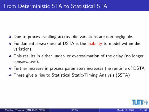
Due to process scalling accross die variations are non-negligible.
Fundamental weakness of DSTA is the inability to model within-dievariations.
This results in either under- or overestimation of the delay (no longerconservative).
Further increase in process parameters increases the runtime of DSTA
These give a rise to Statistical Static-Timing Analysis (SSTA)
Vladimir Todorov (MB-JASS 2009) SSTA March 19, 2009 5 / 31

From Deterministic STA to Statistical STA
Due to process scalling accross die variations are non-negligible.
Fundamental weakness of DSTA is the inability to model within-dievariations.
This results in either under- or overestimation of the delay (no longerconservative).
Further increase in process parameters increases the runtime of DSTA
These give a rise to Statistical Static-Timing Analysis (SSTA)
Vladimir Todorov (MB-JASS 2009) SSTA March 19, 2009 5 / 31

Where are we?
1 IntroductionWhat is Static-Timing Analysis?From Deterministic STA to Statistical STA
2 Statistical Static-Timing AnalysisSources of Timing VariationImpact of Variation on Circuit DelayProblem Formulation and Basic ApproachesSSTA Solution ApproachesBlock-based SSTA
3 Conclusion
Vladimir Todorov (MB-JASS 2009) SSTA March 19, 2009 6 / 31

Sources of Timing Variation
There are three sources of timing variation that need to be considered:
Model Uncertainty
Process Uncertainty
Environment Uncertainty
Model Uncertainty Process Uncertainty Environment Uncertainty
Vladimir Todorov (MB-JASS 2009) SSTA March 19, 2009 7 / 31

Sources of Timing Variation
There are three sources of timing variation that need to be considered:
Model UncertaintyInaccuracy in device models used, extraction and reduction ofinterconnect parasitics and timing-analysis algorithms
Process Uncertainty
Environment Uncertainty
Model Uncertainty Process Uncertainty Environment Uncertainty
Vladimir Todorov (MB-JASS 2009) SSTA March 19, 2009 7 / 31

Sources of Timing Variation
There are three sources of timing variation that need to be considered:
Model Uncertainty
Process UncertaintyUncertainty in the parameters of fabricated devices and interconnects(die-to-die and within-die)
Environment Uncertainty
Model Uncertainty Process Uncertainty Environment Uncertainty
Vladimir Todorov (MB-JASS 2009) SSTA March 19, 2009 7 / 31

Sources of Timing Variation
There are three sources of timing variation that need to be considered:
Model Uncertainty
Process Uncertainty
Environment UncertaintyUncertainty in the operating environment of a device: temperature,operating voltage, mode of operation, lifetime wear-out
Model Uncertainty Process Uncertainty Environment Uncertainty
Vladimir Todorov (MB-JASS 2009) SSTA March 19, 2009 7 / 31

Sources of Process Variation
PhysicalParameterVariations
−→ElectricalParameterVariations
−→DelayVariations
A
Critical DimensionOxide ThicknessChannel DopingWire WidthWire Thickness
−→Saturation CurrentGate CapacitanceTreshold VoltageWire CapacitanceWire Resistance
−→Gate DelaySlew RateWire Delay
Variations are Correlated
Physical variations are result of process variations and may becorrelated as one process variation may result in many physical.
Electrical variations are also correlated as one physical variation mayresult in more than one electrical variation. (Ex. R and C arenegatively correlated with respect to wire width.)
Vladimir Todorov (MB-JASS 2009) SSTA March 19, 2009 8 / 31

Sources of Process Variation
PhysicalParameterVariations
−→ElectricalParameterVariations
−→DelayVariations
A
Critical DimensionOxide ThicknessChannel DopingWire WidthWire Thickness
−→
Saturation CurrentGate CapacitanceTreshold VoltageWire CapacitanceWire Resistance
−→
Gate DelaySlew RateWire Delay
Variations are Correlated
Physical variations are result of process variations and may becorrelated as one process variation may result in many physical.
Electrical variations are also correlated as one physical variation mayresult in more than one electrical variation. (Ex. R and C arenegatively correlated with respect to wire width.)
Vladimir Todorov (MB-JASS 2009) SSTA March 19, 2009 8 / 31

Classification of Physical Variations
Physical variations may be character-ized as either deterministic or statisti-cal.
Vladimir Todorov (MB-JASS 2009) SSTA March 19, 2009 9 / 31

Classification of Physical Variations
Follow well understood behavior.
Predicted upfront by analyzingthe design layout
Arise due to proximity effectsand chemical metal polishing.
Deterministic treatment at laterstages of the design.
Advantageous to treat themstatistically at early stages.
Vladimir Todorov (MB-JASS 2009) SSTA March 19, 2009 9 / 31

Classification of Physical Variations
Truly uncertain component ofvariation.
Result from processesorthogonal to designimplementation.
Only statistics are known atdesign time.
Modeled as random variables(RVs).
Vladimir Todorov (MB-JASS 2009) SSTA March 19, 2009 9 / 31

Classification of Physical Variations
Affect all devices on the samedie in the same way.
Result in shifts that occur fromlot to lot, wafer to wafer, reticleto reticle and accross a reticle.
Vladimir Todorov (MB-JASS 2009) SSTA March 19, 2009 9 / 31
Classification of Physical Variations
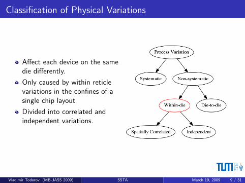
Affect each device on the samedie differently.
Only caused by within reticlevariations in the confines of asingle chip layout
Divided into correlated andindependent variations.
Vladimir Todorov (MB-JASS 2009) SSTA March 19, 2009 9 / 31

Classification of Physical Variations
Processes that cause within dievariation change gradually withposition
Affect closely spaced devices insimilar manner (these exhibitsimilar characteristics)
Referred to as SpatiallyCorrelated Variation.
Vladimir Todorov (MB-JASS 2009) SSTA March 19, 2009 9 / 31

Classification of Physical Variations
The residual variability of adevice that is statisticallyindependent of all other devices
Increasing effect with continuedprocess scalling.
Examples are line-edgeroughtness and random-dopantfluctuations.
Vladimir Todorov (MB-JASS 2009) SSTA March 19, 2009 9 / 31

Impact of Variation on Circuit Delay
Single Path Delay
P1 P2 P3 P4 . . . Pn
Gates connected in series with delay probabilities Pi
Delays-normally distributed and independent with mean µ andvariance σ2
The total delay distribution results in the sum of the distributions onthe path
n∑i=1
N (µ, σ2) = N
(n∑
i=1
µ,
n∑i=1
σ2
)= N (nµ, nσ2)
Which results in total coefficient of variation(σ
µ
)path
=
√nσ2
nµ=
1√n
(σ
µ
)gate
Vladimir Todorov (MB-JASS 2009) SSTA March 19, 2009 10 / 31

Impact of Variation on Circuit Delay
Single Path Delay
P1 P2 P3 P4 . . . Pn
Gates connected in series with delay probabilities Pi
Delays-normally distributed and correlated with mean µ, variance σ2
and correlation coefficient ρ
The total delay distribution results in the sum of the distributions onthe path
µpath = nµ
σ2path =
n∑i=1
σ2 + 2ρn∑
i=1
n∑j>i
σiσj = nσ2(1 + ρ(n − 1))
Which results in total coefficient of variation(σ
µ
)path
=
√nσ2(1 + ρ(n − 1))
nµ=
√1 + ρ(n − 1)
n
(σ
µ
)gate
Vladimir Todorov (MB-JASS 2009) SSTA March 19, 2009 11 / 31

Impact of Variation on Circuit Delay
Single Path Delay
P1 P2 P3 P4 . . . Pn
Gates connected in series with delay probabilities Pi
Delays-normally distributed and correlated with mean µ, variance σ2
and correlation coefficient ρThe total delay distribution results in the sum of the distributions onthe path
µpath = nµ
σ2path =
n∑i=1
σ2 + 2ρn∑
i=1
n∑j>i
σiσj = nσ2(1 + ρ(n − 1))
Which results in total coefficient of variation(σ
µ
)path
=
√nσ2(1 + ρ(n − 1))
nµ=
√1 + ρ(n − 1)
n
(σ
µ
)gate
Vladimir Todorov (MB-JASS 2009) SSTA March 19, 2009 11 / 31

Impact of Variation on Circuit Delay
Maximum Delay of Multiple Paths
Two paths with equal delaydistributions
Three cases are considered:
ρ = 0ρ = 0.5ρ = 1
The independent caseoverestimates the delay
Vladimir Todorov (MB-JASS 2009) SSTA March 19, 2009 12 / 31

Impact of Variation on Circuit Delay
Impact of Assumptions
The independent assumption will underestimate the spread of singlepath delay and will overestimate the maximum of delay of multiplepaths.
The correlated assumption will overestimate the spread of single pathdelay and will underestimate the maximum delay of multiple paths.
Assumptions may be based on circuit topology.
Vladimir Todorov (MB-JASS 2009) SSTA March 19, 2009 13 / 31

Problem Formulation
DAG G = {N,E , ns , nf }N set of nodes (in/outpins)E set of edges withweights di
ns , nf source and sink
If di are RVs then the totaldelay is RV as well
Definition:Let pi be a path of ordered edges from source to sink in G.
Let Di =Pk dij
be the path length of pi .
Then Dmax = max(D1, . . . , Di , . . . , Dn) is referred asthe SSTA problem of the circuit.
Figure taken from the original paper Static-TimingAnalysis: From Basic Principles to State of the Art
Vladimir Todorov (MB-JASS 2009) SSTA March 19, 2009 14 / 31

Problem Formulation
Figure taken from the original paper Static-Timing Analysis: From Basic Principles to State of the Art
Vladimir Todorov (MB-JASS 2009) SSTA March 19, 2009 15 / 31

Challenges in SSTA
Topological Correlation
Caused by reconvergent pathsComplicates the max(. . . )
Spatial Correlation
Due to device proximityHow to model gate delays andarrival times in order toexpress the parametercorrelation?How to propagate andpreserve the correlationinformation?
Vladimir Todorov (MB-JASS 2009) SSTA March 19, 2009 16 / 31

Challenges in SSTA
Nonnormal Process Parameters and Non-linear Delay Models
Nonnormal physical variations exist.Dependence of electrical parameters can be nonlinear.Due to reduction of geometries linear assumption no longer applies.
Skewness due to Maximum Operation
Maximum operation is nonlinear, henceNormal arrival times will result in nonnormal delayMaximum operation which can operate on nonnormal delays is desiredSimply ignoring the skewness introduces error
Vladimir Todorov (MB-JASS 2009) SSTA March 19, 2009 17 / 31

Skewness due to Maximal Operation
Two arrival times with same mean, but different variance result in apositively skewed maximum delay.
Vladimir Todorov (MB-JASS 2009) SSTA March 19, 2009 18 / 31

Skewness due to Maximal Operation
Identically distributed arrival times result in slightly positively skeweddistribution.
Vladimir Todorov (MB-JASS 2009) SSTA March 19, 2009 18 / 31

Skewness due to Maximal Operation
The maximum can safely be assumed to be the distribution with thegreater mean.
Vladimir Todorov (MB-JASS 2009) SSTA March 19, 2009 18 / 31

SSTA Solution Approaches
Numerical Integration
Most generalComputationally expensive
Monte Carlo Methods
Statistical sampling of the sample spacePerform deterministic computation for each sampleAgregate these results into a final result
Probabilistic Analysis Methods
Path-based ApproachBlock-based Approach
Vladimir Todorov (MB-JASS 2009) SSTA March 19, 2009 19 / 31

Probabilistic Analysis Methods
Path-based Approach Block-based Approach
How it works. . .
Set of likely to becomecritical paths
Compute the delay foreach path
Perform a statisticalmaximum
Problems. . .
Difficult to construct setof suitable paths
High computationalefforts for balancedcircuits
−→
How it works. . .
For all fan-in edges theedge delay is added to thearrival time at the sourcenode
Given the resulting timesthe final arrival time atthe node is computedusing maximum operation
Propagates exactly 2arrival times(rise and fall)
Vladimir Todorov (MB-JASS 2009) SSTA March 19, 2009 20 / 31

Distribution Propagation Approaches
Propagation of Sampled and Renormalized Distributions
Computed using discrete sum and maximum
Summation is done by combining multiple shifted values of thedelay
z = x + y
Maximum is taken by evaluatig the probability
z = max(x , y)
fz(t) = Fx(τ < t)fy (t) + Fy (τ < t)fx(t)
Vladimir Todorov (MB-JASS 2009) SSTA March 19, 2009 21 / 31

Distribution Propagation Approaches
Propagation of Sampled and Renormalized Distributions
Computed using discrete sum and maximum
Summation is done by combining multiple shifted values of thedelay
fz(t) = fx(1)fy (t − 1) + fx(2)fy (t − 2) + · · ·+ fz(n)fy (t − n)
Maximum is taken by evaluatig the probability
z = max(x , y)
fz(t) = Fx(τ < t)fy (t) + Fy (τ < t)fx(t)
Vladimir Todorov (MB-JASS 2009) SSTA March 19, 2009 21 / 31

Distribution Propagation Approaches
Propagation of Sampled and Renormalized Distributions
Computed using discrete sum and maximum
Summation is done by combining multiple shifted values of thedelay
fz(t) =∞∑
i=−∞
fx(i)fy (t − i)
Maximum is taken by evaluatig the probability
z = max(x , y)
fz(t) = Fx(τ < t)fy (t) + Fy (τ < t)fx(t)
Vladimir Todorov (MB-JASS 2009) SSTA March 19, 2009 21 / 31

Distribution Propagation Approaches
Propagation of Sampled and Renormalized Distributions
Computed using discrete sum and maximum
Summation is done by combining multiple shifted values of thedelay
fz(t) =∞∑
i=−∞
fx(i)fy (t − i) = fx(t) ∗ fy (t)
Maximum is taken by evaluatig the probability
z = max(x , y)
fz(t) = Fx(τ < t)fy (t) + Fy (τ < t)fx(t)
Vladimir Todorov (MB-JASS 2009) SSTA March 19, 2009 21 / 31

Discrete Distribution Propagation
Vladimir Todorov (MB-JASS 2009) SSTA March 19, 2009 22 / 31

Handling Topological Correlation
Super-Gate
Statistically independent inputsSingle fan-outSeparate propagation of discrete events (enumeration) ∈ O(cn)
Ignoring Topological Correlations
Exists a pdf Q(t) which upper-bounds P(t) for all tResults in pessimistic analysisOriginal P(t) can be approximated by upper and lower bounds
Vladimir Todorov (MB-JASS 2009) SSTA March 19, 2009 23 / 31

Correlation Models (Parameter Space)
Grid Model
Divide the die by a square gridEach square corresponds to agroup of fully correlateddevicesEach square is a RV and iscorrelated to all other squaresConstruct a new set of RVsby whiteningExpress the old set as a linearcombination of the new one
Vladimir Todorov (MB-JASS 2009) SSTA March 19, 2009 24 / 31

Correlation Models (Parameter Space)
Quadtree Model
Recursively divide the die areainto 4Each partition is assigned toan independent RVExpress the correlationvariation by summing the RVof the gate with the onesfrom higher levelsCorrelation arises from sharingRVs on higher levels
Vladimir Todorov (MB-JASS 2009) SSTA March 19, 2009 24 / 31

Propagation of Delay Dependence (Parameter Space)
Canonical form of the delay
da = µa +n∑i
aizi + an+1R
Express the sum in a canonical form
C = A + B
µc = µa + µb
ci = ai + bi for 1 ≤ i ≤ n
cn+1 =√
a2n+1 + b2
n+1
Vladimir Todorov (MB-JASS 2009) SSTA March 19, 2009 25 / 31

Propagation of Delay Dependence (Parameter Space)
Canonical form of the delay
da = µa +n∑i
aizi + an+1R
Express the sum in a canonical form
C = A + B
µc = µa + µb
ci = ai + bi for 1 ≤ i ≤ n
cn+1 =√
a2n+1 + b2
n+1
Vladimir Todorov (MB-JASS 2009) SSTA March 19, 2009 25 / 31

Propagation of Delay Dependence (Parameter Space)
Express the maxium in a canonical form1 Compute variance and covariance of A and B
σ2a =
n∑i
a2i σ2
b =n∑i
b2i r =
n∑i
aibi
2 Compute the tightness probability TA = Pr(A > B)
TA = Φ
(µa − µb
θ
)Φ(x ′) =
∫ x′
−∞φ(x)dx
φ(x) =1√2π
exp−x2
2
θ =√σ2
a + σ2b − 2r
Vladimir Todorov (MB-JASS 2009) SSTA March 19, 2009 26 / 31

Propagation of Delay Dependence (Parameter Space)
Express the maxium in a canonical form
3 Compute mean and variance of C = max(A,B)
µc = µaTA + µb(1− TA) + θφ
(µa − µb
θ
)σ2
c = (µa + σ2a)TA + (µb + σ2
b)(1− TA) + (µa + µb)θφ
(µa − µb
θ
)− µ2
c
4 Compute sensitivity coefficients ci
ci = aiTA + bi (1− TA) for 1 ≤ i ≤ n
5 Compute cn+1 of Capprox to get a consistent estimate
Vladimir Todorov (MB-JASS 2009) SSTA March 19, 2009 26 / 31

Propagation of Delay Dependence (Parameter Space)
Capprox is only approximation and is not conservative
Therefore, by the use of the relationship
max
(n∑i
ai ,
n∑i
bi
)≤
n∑i
max(ai , bi )
Cbound can be constructed which is conservative
µc = max(µa, µb)
cboundi= max(ai , bi )
Vladimir Todorov (MB-JASS 2009) SSTA March 19, 2009 27 / 31

Nonlinear and Nonnormal Approaches
Nonlinear device dependencies
da = µa +n∑i
aizi +n∑
i=1
n∑j=1
bijzizj + an+1R
Nonnormal physical or electrical variations
da = µa +n∑i
aizi +m∑j
an+jzn+j + an+m+1R
Generalized in
da = µa +n∑i
aizi + f(zn+1, . . . , zn+m) + an+1R
Handled by numerical computations and tightness probabilities
Vladimir Todorov (MB-JASS 2009) SSTA March 19, 2009 28 / 31

Where are we?
1 IntroductionWhat is Static-Timing Analysis?From Deterministic STA to Statistical STA
2 Statistical Static-Timing AnalysisSources of Timing VariationImpact of Variation on Circuit DelayProblem Formulation and Basic ApproachesSSTA Solution ApproachesBlock-based SSTA
3 Conclusion
Vladimir Todorov (MB-JASS 2009) SSTA March 19, 2009 29 / 31

Conclusion
SSTA has gained excessive interest in recent years
Currently a number of commercial efforts are underway
However, state-of-the-art SSTA does not address many of the issuestaken for granted in DSTA
Coupling noiseClock issuesComplex delay modelling
SSTA must move beyound analysis into optimization
Vladimir Todorov (MB-JASS 2009) SSTA March 19, 2009 30 / 31

Discussion
. . .
Vladimir Todorov (MB-JASS 2009) SSTA March 19, 2009 31 / 31


![Statistical Static-Timing Analysis: From Basic Principles …€¦ · Statistical Static-Timing Analysis: From Basic Principles to State of the Art [1] Vladimir Todorov Moscow-Bavarian](https://static.fdocuments.us/doc/165x107/5b7c163b7f8b9a004b8e1068/statistical-static-timing-analysis-from-basic-principles-statistical-static-timing.jpg)