STATIC PUSHOVER ANALYSISSTATIC PUSHOVER ANALYSIS ZSoilr.PC 070202 report by A. Urbanski E. Spacone...

STATIC PUSHOVER ANALYSISZSoilr.PC 070202 report

byA. UrbanskiE. SpaconeM. BelgasmiaJ.-L. SarfTh. Zimmermann

Zace Services Ltd, Software engineering

P.O.Box 224, CH-1028 Prverenges

Switzerland

(T) +41 21 802 46 05

(F) +41 21 802 46 06

http://www.zsoil.com,

hotline: [email protected]

since 1985

ii ZSoilr.PC 070202 report

Contents

1 INTRODUCTION 3

2 NONLINEAR FRAME ANALYSIS METHODS IN EUROCODE 8 5

3 NONLINEAR STATIC PUSHOVER ANALYSIS ACCORDING TO EUROCODE8 7

3.1 Equivalent SDOF model and capacity diagram in Eurocode 8 . . . . . . . . 8

3.2 Linearization of the capacity curve and comparison to demand spectrum . . . 11

3.2.1 Linearization of the capacity curve . . . . . . . . . . . . . . . . . . 11

3.2.2 Seismic demand . . . . . . . . . . . . . . . . . . . . . . . . . . . . 13

3.3 Summary of nonlinear static pushover analysis in Eurocode 8 . . . . . . . . . 17

3.4 Accidental torsional effects in Eurocode 8 . . . . . . . . . . . . . . . . . . . 18

3.5 Combination of the horizontal seismic action effects according to Eurocode 8 21

4 NONLINEAR MODELING IN EUROCODE 8 23

5 Applications: Study of Bonefro buidling 25

5.1 Bonefro building modeling . . . . . . . . . . . . . . . . . . . . . . . . . . . 26

5.2 Response of Bonefro building to ground acceleration, comparison of force anddisplacement based elements . . . . . . . . . . . . . . . . . . . . . . . . . 27

5.3 Response of Bonefro building to 2D pushover analysis . . . . . . . . . . . . 27

5.4 Nonlinear pushover on 3D frame with ZSoilr (small displacements) . . . . . 29

5.5 Simulated accelerograms . . . . . . . . . . . . . . . . . . . . . . . . . . . . 31

5.6 Nonlinear time history analysis of 3D model . . . . . . . . . . . . . . . . . . 32

5.7 Sensitivity to seismic parameters . . . . . . . . . . . . . . . . . . . . . . . . 33

5.8 Sensitivity of response to large deformation . . . . . . . . . . . . . . . . . . 34

5.9 Observations . . . . . . . . . . . . . . . . . . . . . . . . . . . . . . . . . . 34

6 Data preparation for pushover analysis in ZSoilr.PC 37

CONTENTS

6.1 Control . . . . . . . . . . . . . . . . . . . . . . . . . . . . . . . . . . . . . 38

6.2 Modeling of masses . . . . . . . . . . . . . . . . . . . . . . . . . . . . . . 40

6.3 Selection of a control node . . . . . . . . . . . . . . . . . . . . . . . . . . 41

6.4 Results . . . . . . . . . . . . . . . . . . . . . . . . . . . . . . . . . . . . 41

6.5 Pushover results . . . . . . . . . . . . . . . . . . . . . . . . . . . . . . . . 42

6.6 Postprocessing . . . . . . . . . . . . . . . . . . . . . . . . . . . . . . . . . 45

ZSoilr.PC 070202 report 1

CONTENTS

2 ZSoilr.PC 070202 report

Chapter 1

INTRODUCTION

Modern seismic design codes allow engineers to use either linear or nonlinear analyses tocompute design forces and design displacements. In particular, Eurocode 8 contains fourmethods of analysis: linear simplified static analysis, linear modal analysis, nonlinear pushoveranalysis and nonlinear time-history analysis. These methods refer to the design and analysis offramed structures, mainly buildings and bridges. The two nonlinear methods require advancedmodels and advanced nonlinear procedures in order to be fully applicable by design engineers.This report gives an introduction to the use of PUSHOVER analysis with ZSOIL.

Displacement-based and force-base elements are used in this study. The first is a classicaltwo-node, displacement-based, Euler-Bernoulli frame element. The second is a two-node,force-based, Euler Bernoulli frame element. The main advantage of the second element isthat it is “exact” within the relevant frame element theory. This implies that one elementper frame member (beam or column) is used in preparing the frame mesh, thus leadingto a reduction of the global number of degrees of freedom. The complete theory for theforce-based element can be found in (Spacone, 1996).

The nonlinear response of a 2D model of an existing building is presented as an illustration.The building is a residential two-storey reinforced concrete building in Bonefro, Italy. It isrepresentative of typical residential building construction in Italy in the 1970’s and 1980’s.The design spectrum for the building was obtained from EC8 using the local soil propertiesand the peak ground acceleration given by the new Italian seismic map.

This work presents the nonlinear pushover procedure, which is based on the N2 methoddeveloped by Fajfar (Fajfar, 1999). The procedure is illustrated on a 2D model of an existingbuilding and the data structure to perform such analyses in ZSOIL is presented. More detailsand comparisons with dynamic analysis can be found in (Belgasmia & al. 2006)

CHAPTER 1. INTRODUCTION


Chapter 2

NONLINEAR FRAME ANALYSISMETHODS IN EUROCODE 8

In this section the nonlinear pushover procedures given by Eurocode 8 are presented. Pushoveranalysis is described in §4.3.3.4.2. of EC8 Part 1. According to EC8, pushover analysis maybe used to verify the structural performance of newly designed buildings and of existingbuildings. In particular, pushover analysis may be used for the following purposes:

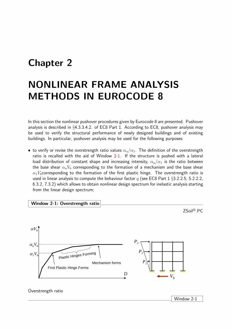
• to verify or revise the overstrength ratio values αu/α1. The definition of the overstrengthratio is recalled with the aid of Window 2-1. If the structure is pushed with a lateralload distribution of constant shape and increasing intensity, αu/α1 is the ratio betweenthe base shear αuVb corresponding to the formation of a mechanism and the base shearα1Vbcorresponding to the formation of the first plastic hinge. The overstrength ratio isused in linear analysis to compute the behaviour factor q (see EC8 Part 1 §3.2.2.5, 5.2.2.2,6.3.2, 7.3.2) which allows to obtain nonlinear design spectrum for inelastic analysis startingfrom the linear design spectrum;

Window 2-1: Overstrength ratio

ZSoilr.PC

D

αVb

First Plastic Hinge Forms

Plastic Hinges Forming

Mechanism forms

Vb

P1

P2

αuVb

α1Vb

P3

Overstrength ratio

Window 2-1

CHAPTER 2. NONLINEAR FRAME ANALYSIS METHODS IN EUROCODE 8

• to estimate the expected plastic mechanisms and the damage distribution;

• to assess the structural performance of existing or retrofitted buildings for the purposes ofEN 1998-3 (EC8 Part 3);

• as an alternative to the design based on linear-elastic analysis which uses the behaviourfactor q. In this case, the target displacement found from the pushover analysis should beused as the basis for the design;

• EC8 Part 1 §4.3.3.4.2.1 adds that buildings not conforming to the regularity criteria of EC8shall be analyzed using a spatial (3D) structural model. Two independent analyses withlateral loads applied in one direction only may be performed. No indications are given inEC8 or in the published literature on how to perform a pushover analysis with two loadsdistributions applied simultaneously in two orthogonal directions, therefore it is assumedhere that in a pushover analysis the structure is pushed with loads applied in one horizontaldirection at a time (the vertical seismic is typically neglected in buildings). Indications aregiven on how to combine the effects of the actions applied separately in two horizontaldirections (EC8 Part 1 §4.3.3.5). For buildings conforming to the regularity criteria of EC8the analysis may be performed using two planar models, one for each principal directionhorizontal direction.

The structural element models and the resulting structural model of the overall building arevery similar for pushover and nonlinear time-history analysis. The only difference lies in theneed to have cyclic models for the time-history analysis.

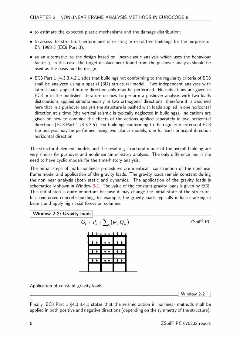
The initial steps of both nonlinear procedures are identical: construction of the nonlinearframe model and application of the gravity loads. The gravity loads remain constant duringthe nonlinear analysis (both static and dynamic). The application of the gravity loads isschematically shown in Window 3-1. The value of the constant gravity loads is given by EC8.This initial step is quite important because it may change the initial state of the structure.In a reinforced concrete building, for example, the gravity loads typically induce cracking inbeams and apply high axial forces on columns.

Window 2-2: Gravity loads

ZSoilr.PC( )2k k i kiiG P Qψ+ +∑

Application of constant gravity loads

Window 2-2

Finally, EC8 Part 1 §4.3.3.4.1 states that the seismic action in nonlinear methods shall beapplied in both positive and negative directions (depending on the symmetry of the structure).


Chapter 3

NONLINEAR STATIC PUSHOVERANALYSIS ACCORDING TOEUROCODE 8

The Nonlinear Static Pushover Procedure in EC8 follows the N2 method developed by Fajfar(1999). The method consists of applying constant load shapes to the building model. Theload shapes represent the lateral loads applied by the ground motion. The load intensity isincreased in a pseudo-static manner. The structure model can be planar (2D) or spatial (3D),depending on the regularity characteristics of the building. The load pattern, on the otherhand, is always applied in one direction only. For analyses with input ground motion in morethan one direction, for example input ground motion in the x and y directions, combinationrules are given by EC8.

The nonlinear pushover analysis consists of applying monotonically increasing constant shapelateral load distributions to the structure under consideration. The structure model can beeither 2D or 3D. In particular, EC8 states that for buildings with plan regularity, 2D analysis ofsingle plane frames can be performed, while for buildings with plan irregularity a complete 3Dmodel is necessary. Given that the nonlinear methods are particularly interesting for existingbuildings, which are rarely regular, a 3D model is required in most cases.

The N2 method was developed using a shear building model, i.e. a frame model with floorsrigid in their planes. Furthermore, vertical displacement are typically neglected in the methodand only the two horizontal ground motion components, x and y, are considered. Extensionto the general case of a fully deformable frame is straightforward. The N2 method consistsof applying two load distributions to the frame:

• a “modal” pattern, that is a load shape proportional to the mass matrix multiplied by thefirst elastic mode shape,

P1 = Mϕ1

• a “uniform” pattern, that is a mass proportional load shape,

P2 = MR

where M is the mass matrix, ϕ1 is the first mode shape and R a vector of 1s correspondingto the degrees of freedom parallel to the application of the ground motion and 0s for all

CHAPTER 3. NONLINEAR STATIC PUSHOVER ANALYSIS

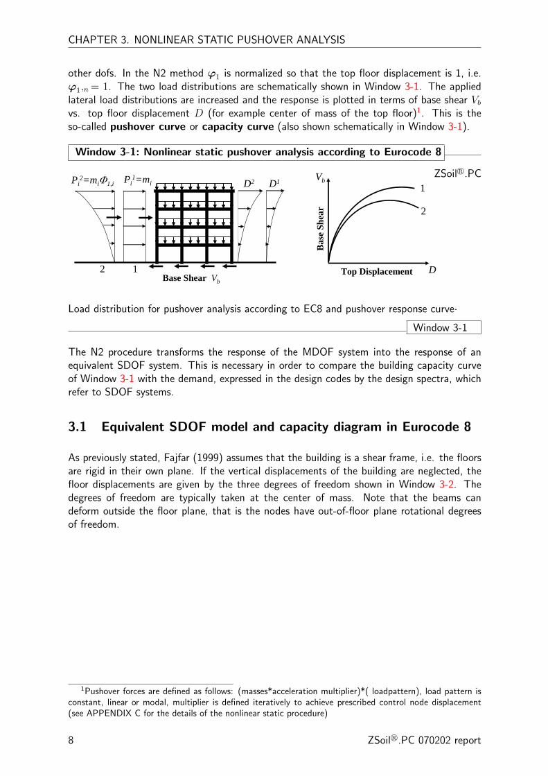
other dofs. In the N2 method ϕ1 is normalized so that the top floor displacement is 1, i.e.ϕ1,n = 1. The two load distributions are schematically shown in Window 3-1. The appliedlateral load distributions are increased and the response is plotted in terms of base shear Vbvs. top floor displacement D (for example center of mass of the top floor)1. This is theso-called pushover curve or capacity curve (also shown schematically in Window 3-1).

Window 3-1: Nonlinear static pushover analysis according to Eurocode 8

ZSoilr.PCD1

1

Pi2=miΦ1,i

2

D2

Bas

e Sh

ear

D

1

2

VbPi1=mi

Top DisplacementBase Shear Vb

Load distribution for pushover analysis according to EC8 and pushover response curve·

Window 3-1

The N2 procedure transforms the response of the MDOF system into the response of anequivalent SDOF system. This is necessary in order to compare the building capacity curveof Window 3-1 with the demand, expressed in the design codes by the design spectra, whichrefer to SDOF systems.

3.1 Equivalent SDOF model and capacity diagram in Eurocode 8

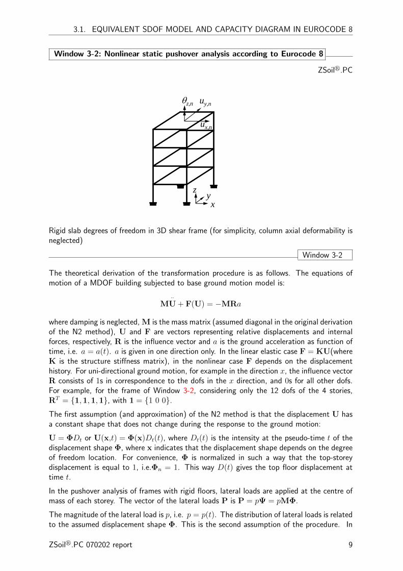
As previously stated, Fajfar (1999) assumes that the building is a shear frame, i.e. the floorsare rigid in their own plane. If the vertical displacements of the building are neglected, thefloor displacements are given by the three degrees of freedom shown in Window 3-2. Thedegrees of freedom are typically taken at the center of mass. Note that the beams candeform outside the floor plane, that is the nodes have out-of-floor plane rotational degreesof freedom.

1Pushover forces are defined as follows: (masses*acceleration multiplier)*( loadpattern), load pattern isconstant, linear or modal, multiplier is defined iteratively to achieve prescribed control node displacement(see APPENDIX C for the details of the nonlinear static procedure)


3.1. EQUIVALENT SDOF MODEL AND CAPACITY DIAGRAM IN EUROCODE 8

Window 3-2: Nonlinear static pushover analysis according to Eurocode 8

ZSoilr.PC

xyz

ux,n

uy,nθz,n

Rigid slab degrees of freedom in 3D shear frame (for simplicity, column axial deformability isneglected)

Window 3-2

The theoretical derivation of the transformation procedure is as follows. The equations ofmotion of a MDOF building subjected to base ground motion model is:

M··U + F(U) = −MRa

where damping is neglected, M is the mass matrix (assumed diagonal in the original derivationof the N2 method), U and F are vectors representing relative displacements and internalforces, respectively, R is the influence vector and a is the ground acceleration as function oftime, i.e. a = a(t). a is given in one direction only. In the linear elastic case F = KU(whereK is the structure stiffness matrix), in the nonlinear case F depends on the displacementhistory. For uni-directional ground motion, for example in the direction x, the influence vectorR consists of 1s in correspondence to the dofs in the x direction, and 0s for all other dofs.For example, for the frame of Window 3-2, considering only the 12 dofs of the 4 stories,RT = {1,1,1,1}, with 1 = {1 0 0}.

The first assumption (and approximation) of the N2 method is that the displacement U hasa constant shape that does not change during the response to the ground motion:

U = ΦDt or U(x,t) = Φ(x)Dt(t), where Dt(t) is the intensity at the pseudo-time t of thedisplacement shape Φ, where x indicates that the displacement shape depends on the degreeof freedom location. For convenience, Φ is normalized in such a way that the top-storeydisplacement is equal to 1, i.e.Φn = 1. This way D(t) gives the top floor displacement attime t.

In the pushover analysis of frames with rigid floors, lateral loads are applied at the centre ofmass of each storey. The vector of the lateral loads P is P = pΨ = pMΦ.

The magnitude of the lateral load is p, i.e. p = p(t). The distribution of lateral loads is relatedto the assumed displacement shape Φ. This is the second assumption of the procedure. In



more complex models with deformable slabs and with distributed masses at each node theload, the load vector P is applied to all degrees of freedoms with mass in the direction ofthe applied ground motion. Note that the displacement shape Φ is needed only for thetransformation from the MDOF system to the equivalent SDOF system of the nonlinearpushover procedure. In the general case of a 3D building, Φ has nonzero components in thesix dofs of each node.

From above equations it follows that in a shear frame the lateral force in the i-th storey isproportional to the component Φi of the assumed displacement, weighted by the storey massmi. If the ground motion is applied in the x direction Pi = pmiΦxi

From statics it follows that P = F, that is the internal forces F are equal to the pseudo-staticexternal forces P.

By combining the above equations and by pre-multiplying by ΦT , we obtain

ΦTMΦ··Dt + ΦTMΦp = ΦTMRa

The left term of Equation is then divided and multiplied by ΦTMR to obtain

ΦTMR︸︷︷︸m∗

ΦTMΦ

ΦTMR︸︷︷︸1Γ

··Dt +

ΦTMΦ

ΦTMR︸︷︷︸1Γ

ΦTMRp︸︷︷︸Vb

= ΦTMR︸︷︷︸m∗

a

where m∗ is the mass of the SDOF equivalent to the MDOF building

m∗ = ΦTMR

For a shear building and ground motion applied in the x direction:

m∗ =∑

miΦx,i

where Φx,i is x component of the modal shape vector for node i. The constant Γ controlsthe transformation from MDOF to SDOF and back:

Γ =ΦTMR

ΦTMΦ

For a shear building and ground motion in the x direction:

Γ =

∑miΦx,i∑miΦ2

x,i

Γ is a factor that, for Φ equal to the mode shape of one of the building’s modes, correspondsto the mode participation factor. In the development of the N2 method, can be any reasonabledeformed shape.

Vb is the base shear of the MDOF building in the direction of the ground motion, equal to:

Vb = ΦTMRp

For a shear building and ground motion applied in the x direction:

Vx = p∑

miΦx,i =∑

Px,i


3.1. LINEARIZATION OF THE CAPACITY CURVE

Window 3-3: Transformation from response of MDOF to equivalent SDOF

ZSoilr.PC

Vb

D

Vb

D

*

*

bVF

DD

=Γ

=Γ

*F

*D

*F

*DΓ

M RM

T

T= ΦΦ Φ

Capacity curve: transformation from response of MDOF to equivalent SDOF

Window 3-3

The equation the SDOF equivalent to the MODF building is thus obtained:

D∗ =Dt

Γ, F ∗ =

VbΓ

The above derivation allows the transformation of the MDOF pushover capacity curves ofWindow 3-1 into pushover curves for the equivalent SDOF system, as shown in Window 3-3

Both force and displacement axes are scaled by the same factor Γ. The stiffness of the systemremains the same. Note that the transformation factor Γ depends on the shape Φ of theassumed displacement shape, and is thus different for different choices of Φ. As shown inWindow 3-1, two forms of loadings are suggested in EC8:

a) Φ = Φ1, thus Γ =ΦT

1 MR

ΦT1 MΦ1

,

b) Φ = R thus Γ = 1.

3.2 Linearization of the capacity curve and comparison to demandspectrum

3.2.1 Linearization of the capacity curve

In order to compare the capacity curve to the demand curve given by the design spectrum,the nonlinear pushover curves of the SDOF are approximated by elastic-perfectly plastic(or bilinear) curves. According to Annex B if the draft EC8 0 this transformation can bebased on the equal energy principle. A target displacement is assumed, and equal energy isassumed between bilinear and nonlinear pushover curves. This simple procedure is illustratedin Window 3-4.



Window 3-4: Linearization of the capacity curve

ZSoilr.PC

*F*yF

*D*yD *

mD

*F

*D*mD

*mE

Bilinearization of the capacity curve of SDOF

Window 3-4

The bilinearization of Window 3-4 gives the yield force and the yield displacement

D∗y = 2

(D∗m −

E∗m

F ∗y

),

which allow the initial elastic period to be computed as:

T ∗ = 2π

√m∗D∗

y

F ∗y

.

Secondly, the capacity curve is transformed into capacity spectrum by normalizing the forcewith respect to the SDOF weight. The resulting capacity spectrum is shown in Window 3-5.

Window 3-5: Capacity spectrum

ZSoilr.PC

*D*yD *

mD

*

*F

mg

SDOF capacity spectrum

Window 3-5



3.2.2 Seismic demand

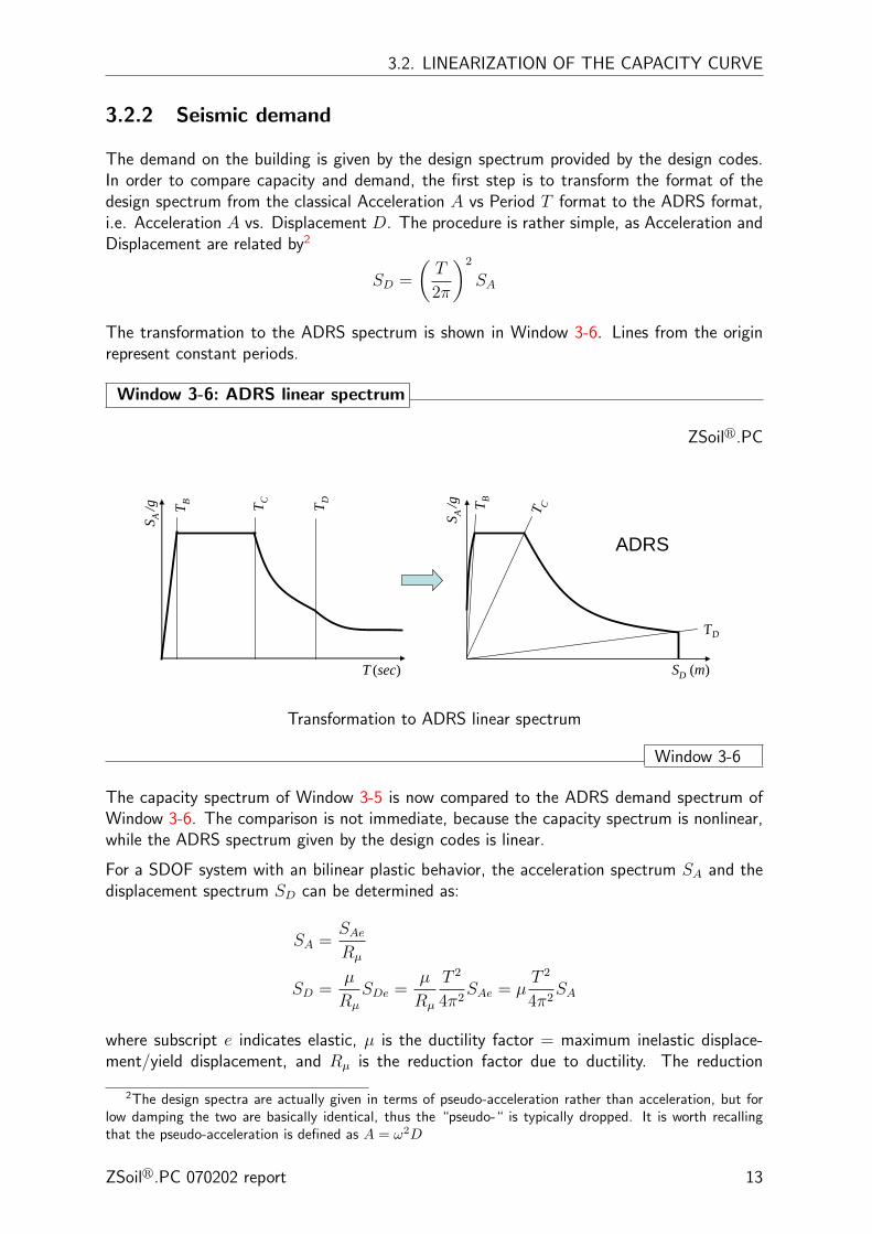
The demand on the building is given by the design spectrum provided by the design codes.In order to compare capacity and demand, the first step is to transform the format of thedesign spectrum from the classical Acceleration A vs Period T format to the ADRS format,i.e. Acceleration A vs. Displacement D. The procedure is rather simple, as Acceleration andDisplacement are related by2

SD =

(T

2π

)2

SA

The transformation to the ADRS spectrum is shown in Window 3-6. Lines from the originrepresent constant periods.

Window 3-6: ADRS linear spectrum

ZSoilr.PC

T (sec)

S A /g T B T C T D

SD (m)

S A /g

TD

T CT B

ADRS

Transformation to ADRS linear spectrum

Window 3-6

The capacity spectrum of Window 3-5 is now compared to the ADRS demand spectrum ofWindow 3-6. The comparison is not immediate, because the capacity spectrum is nonlinear,while the ADRS spectrum given by the design codes is linear.

For a SDOF system with an bilinear plastic behavior, the acceleration spectrum SA and thedisplacement spectrum SD can be determined as:

SA =SAeRµ

SD =µ

Rµ

SDe =µ

Rµ

T 2

4π2SAe = µ

T 2

4π2SA

where subscript e indicates elastic, µ is the ductility factor = maximum inelastic displace-ment/yield displacement, and Rµ is the reduction factor due to ductility. The reduction

2The design spectra are actually given in terms of pseudo-acceleration rather than acceleration, but forlow damping the two are basically identical, thus the “pseudo-“ is typically dropped. It is worth recallingthat the pseudo-acceleration is defined as A = ω2D



factor Rµ can be found in different ways, some analytical, other approximated. In the simpleversion of the N2 method, the following approximated expressions are given:

Rµ = (µ− 1)T

TC+ 1, T < TC

Rµ = µ, T ≥ TC

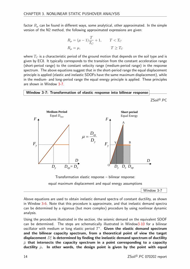
where TC is a characteristic period of the ground motion that depends on the soil type and isgiven by EC8. It typically corresponds to the transition from the constant acceleration range(short-period range) to the constant velocity range (medium-period range) in the responsespectrum. The above equations suggest that in the short-period range the equal displacementprinciple is applied (elastic and inelastic SDOFs have the same maximum displacement), whilein the medium- and long-period range the equal energy principle is applied. These principlesare shown in Window 3-7.

Window 3-7: Transformation of elastic response into bilinear response

ZSoilr.PC

F

D

yF

F

D

yF

O

Y

A

B

Medium PeriodEqual Dmax

Short periodEqual Energy

ep

y

DD

μ =

Dep= DeDy DepDeDy

Transformation elastic response – bilinear response:

equal maximum displacement and equal energy assumptions

Window 3-7

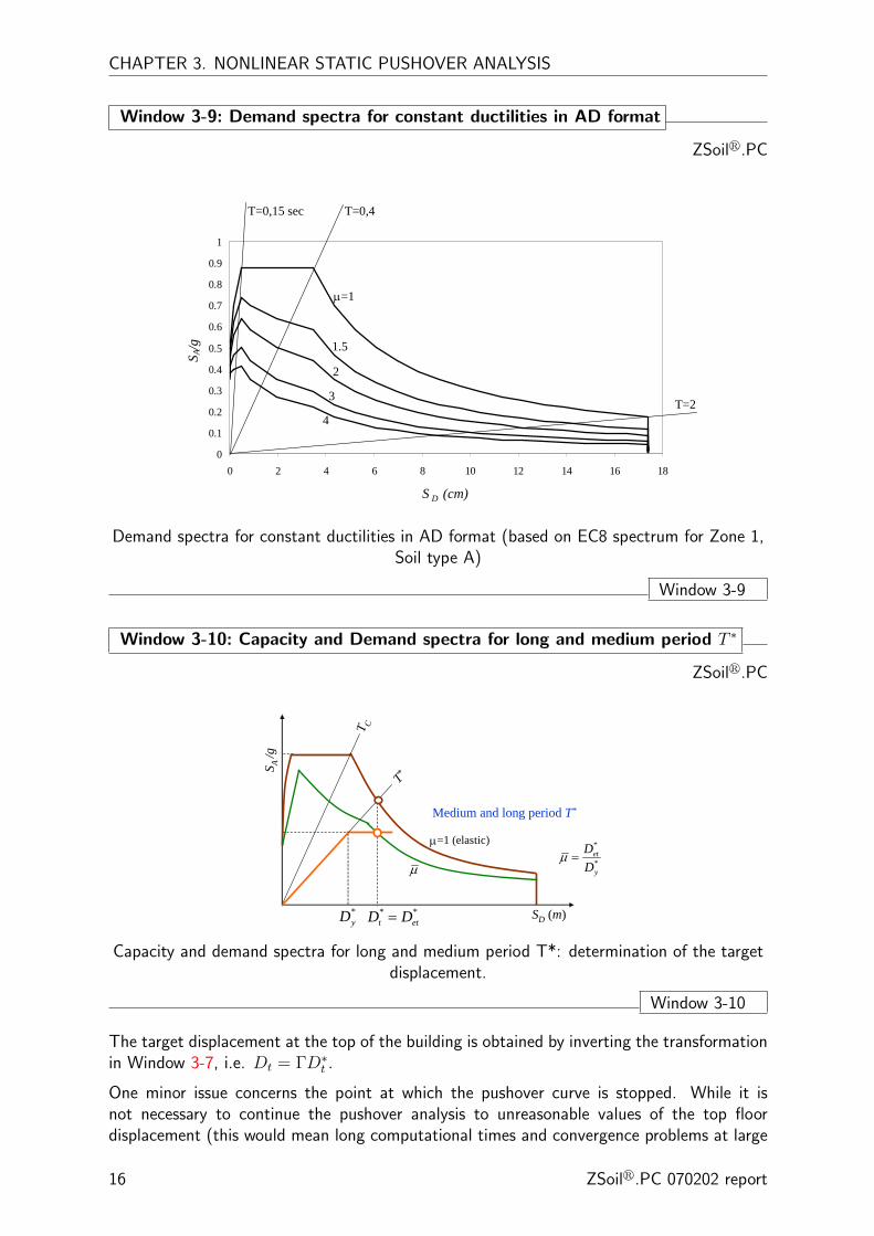
Above equations are used to obtain inelastic demand spectra of constant ductility, as shownin Window 3-6. Note that this procedure is approximate, and that inelastic demand spectracan be determined by a rigorous (but more complex) procedure by using nonlinear dynamicanalysis.

Using the procedures illustrated in the section, the seismic demand on the equivalent SDOFcan be determined. The steps are schematically illustrated in Window3-10 for a bilinearoscillator with medium or long elastic period T ∗. Given the elastic demand spectrumand the bilinear capacity spectrum, from a theoretical point of view the targetdisplacement D∗

t is determined by finding the inelastic demand spectrum of ductilityµ that intersects the capacity spectrum in a point corresponding to a capacityductility µ. In other words, the design point is given by the point with equal



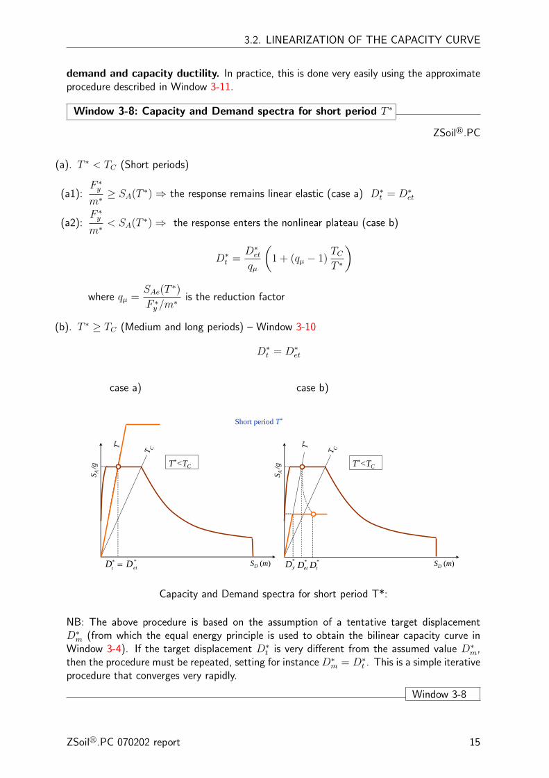
demand and capacity ductility. In practice, this is done very easily using the approximateprocedure described in Window 3-11.

Window 3-8: Capacity and Demand spectra for short period T ∗

ZSoilr.PC

(a). T ∗ < TC (Short periods)

(a1):F ∗y

m∗ ≥ SA(T ∗)⇒ the response remains linear elastic (case a) D∗t = D∗

et

(a2):F ∗y

m∗ < SA(T ∗)⇒ the response enters the nonlinear plateau (case b)

D∗t =

D∗et

qµ

(1 + (qµ − 1)

TCT ∗

)

where qµ =SAe(T

∗)

F ∗y /m

∗ is the reduction factor

(b). T ∗ ≥ TC (Medium and long periods) – Window 3-10

D∗t = D∗

et

case a) case b)

SD (m)

S A /g

T C

T*<TC

T*

*yD *

etD *tDSD (m)

S A /g

T C

T*<TC

T*

*tD D=

Short period T*

*et

Capacity and Demand spectra for short period T*:

NB: The above procedure is based on the assumption of a tentative target displacementD∗m (from which the equal energy principle is used to obtain the bilinear capacity curve in

Window 3-4). If the target displacement D∗t is very different from the assumed value D∗

m,then the procedure must be repeated, setting for instance D∗

m = D∗t . This is a simple iterative

procedure that converges very rapidly.

Window 3-8



Window 3-9: Demand spectra for constant ductilities in AD format

ZSoilr.PC

0

0.1

0.2

0.3

0.4

0.5

0.6

0.7

0.8

0.9

1

0 2 4 6 8 10 12 14 16 18

S D (cm)

S A/g

μ=1

1.5

2

3

4

T=0,15 sec T=0,4

T=2

Demand spectra for constant ductilities in AD format (based on EC8 spectrum for Zone 1,Soil type A)

Window 3-9

Window 3-10: Capacity and Demand spectra for long and medium period T ∗

ZSoilr.PC

SD (m)

S A /g

T C

T*

*yD * *

t etD D=

Medium and long period T*

μ=1 (elastic)

μ

*

*et

y

DD

μ =

Capacity and demand spectra for long and medium period T*: determination of the targetdisplacement.

Window 3-10

The target displacement at the top of the building is obtained by inverting the transformationin Window 3-7, i.e. Dt = ΓD∗

t .

One minor issue concerns the point at which the pushover curve is stopped. While it isnot necessary to continue the pushover analysis to unreasonable values of the top floordisplacement (this would mean long computational times and convergence problems at large


3.3. SUMMARY OF NONLINEAR STATIC PUSHOVER ANALYSIS IN EUROCODE 8

displacement values), there is no general rule on when to stop the pushover curve. This meansthat it may happen that the pushover curve is stopped at a displacement level smaller thatthe computed target displacement. In this case, the pushover analysis must be repeated andit must be stopped at higher top displacement values. It is suggested to push the structureto top-displacements of the order of 2%-3% h, where h is the entire height of the building,for pushover analysis at the Ultimate and Collapse Limit States.

Finally, note that in general for each seismic input direction (x and y), four different pushoveranalysis should be performed. Besides considering two different load shapes (Window 3-1) itis in general necessary to consider the forces applied both with the positive and the negativesign, as the irregularity of the building may lead to different responses in the positive andnegative directions.

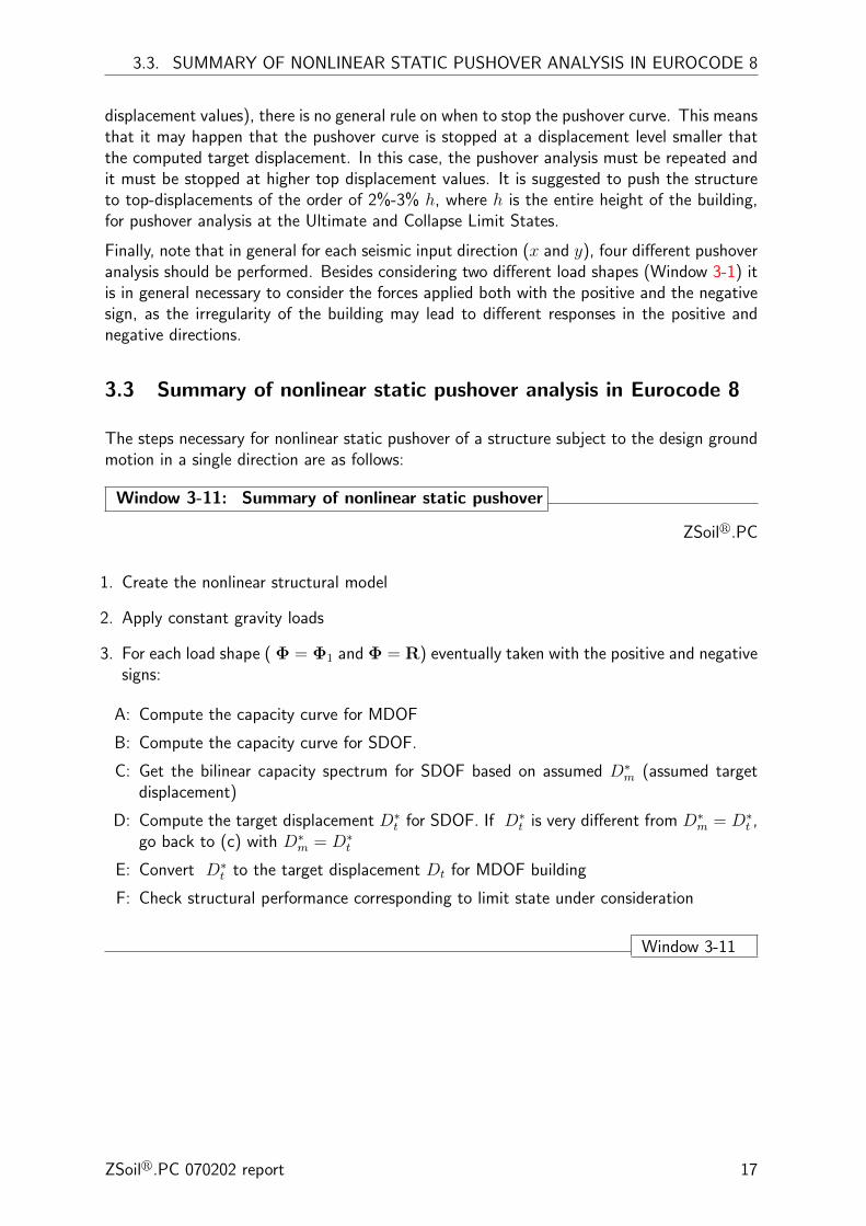
3.3 Summary of nonlinear static pushover analysis in Eurocode 8

The steps necessary for nonlinear static pushover of a structure subject to the design groundmotion in a single direction are as follows:

Window 3-11: Summary of nonlinear static pushover

ZSoilr.PC

1. Create the nonlinear structural model

2. Apply constant gravity loads

3. For each load shape ( Φ = Φ1 and Φ = R) eventually taken with the positive and negativesigns:

A: Compute the capacity curve for MDOF

B: Compute the capacity curve for SDOF.

C: Get the bilinear capacity spectrum for SDOF based on assumed D∗m (assumed target

displacement)

D: Compute the target displacement D∗t for SDOF. If D∗

t is very different from D∗m = D∗

t ,go back to (c) with D∗

m = D∗t

E: Convert D∗t to the target displacement Dt for MDOF building

F: Check structural performance corresponding to limit state under consideration

Window 3-11



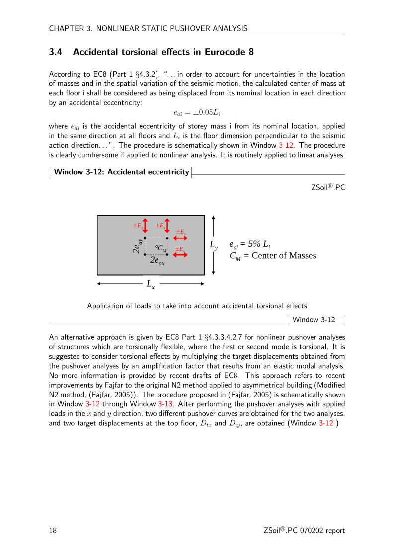
3.4 Accidental torsional effects in Eurocode 8

According to EC8 (Part 1 §4.3.2), “. . . in order to account for uncertainties in the locationof masses and in the spatial variation of the seismic motion, the calculated center of mass ateach floor i shall be considered as being displaced from its nominal location in each directionby an accidental eccentricity:

eai = ±0.05Li

where eai is the accidental eccentricity of storey mass i from its nominal location, appliedin the same direction at all floors and Li is the floor dimension perpendicular to the seismicaction direction. . . ”. The procedure is schematically shown in Window 3-12. The procedureis clearly cumbersome if applied to nonlinear analysis. It is routinely applied to linear analyses.

Window 3-12: Accidental eccentricity

ZSoilr.PC

Lx

LyCM = Center of Masses2eax

2eay eai = 5% Li

xE±

xE±

yE± yE±

CM

Application of loads to take into account accidental torsional effects

Window 3-12

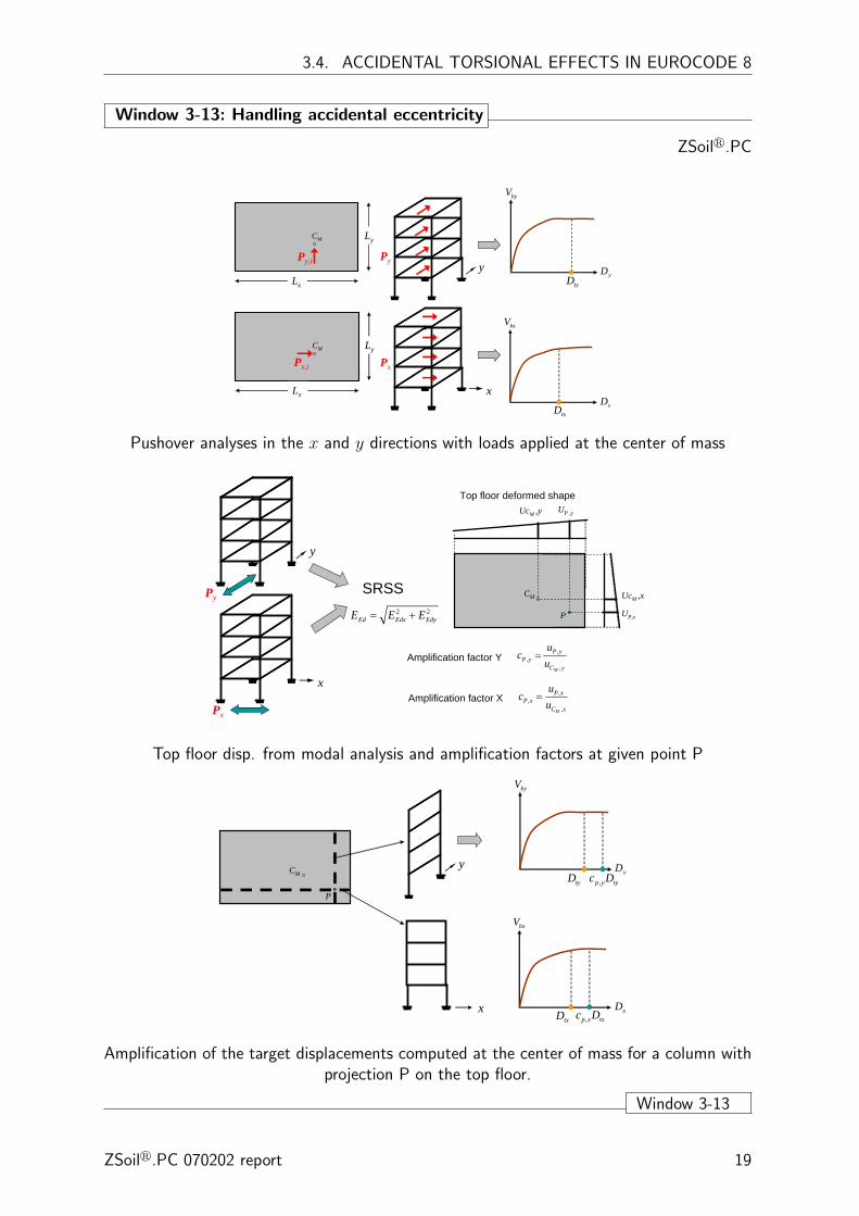
An alternative approach is given by EC8 Part 1 §4.3.3.4.2.7 for nonlinear pushover analysesof structures which are torsionally flexible, where the first or second mode is torsional. It issuggested to consider torsional effects by multiplying the target displacements obtained fromthe pushover analyses by an amplification factor that results from an elastic modal analysis.No more information is provided by recent drafts of EC8. This approach refers to recentimprovements by Fajfar to the original N2 method applied to asymmetrical building (ModifiedN2 method, (Fajfar, 2005)). The procedure proposed in (Fajfar, 2005) is schematically shownin Window 3-12 through Window 3-13. After performing the pushover analyses with appliedloads in the x and y direction, two different pushover curves are obtained for the two analyses,and two target displacements at the top floor, Dtx and Dty, are obtained (Window 3-12 )


3.4. ACCIDENTAL TORSIONAL EFFECTS IN EUROCODE 8

Window 3-13: Handling accidental eccentricity

ZSoilr.PC

Py

Px

y

x

tyD

byV

yD

bxV

xDtxD

Lx

LyCM

Lx

LyCM

Py,i

Px,i

Pushover analyses in the x and y directions with loads applied at the center of mass

Py

Px

y

x

2 2Ed Edx EdyE E E= +

SRSS CM

UcM ,y

UcM ,x

P

UP ,y

UP,x

Amplification factor Y

Amplification factor X ,,

,M

P xP x

C x

uc

u=

,,

,M

P yP y

C y

uc

u=

Top floor deformed shape

Top floor disp. from modal analysis and amplification factors at given point P

yCM

PtyD

byV

yD

bxV

xDtxD

,p y tyc D

,p x txc Dx

Amplification of the target displacements computed at the center of mass for a column withprojection P on the top floor.

Window 3-13



The target displacements Dtx and Dty are multiplied by and amplification factor obtainedfrom the modal analysis of the building. This is schematically shown in Window3-13 Fig 2.Given for example a column passing through point P, amplification factors are computed forthis point. The amplification factors cP ,x and cP ,y, different for the x and y directions, aregiven by the ratios between the displacements of point P ((uP ,x and uP ,y for the x and ydirections, respectively) and the displacements of top floor center of mass (uCM ,x and uCM ,yfor the x and y directions, respectively):

cP ,x =uP ,xuCM ,x

cP ,y =uP ,yuCM ,y

The target displacements for which the column passing through point P is checked are thenmodified to the values cP ,xDtx and cP ,yDty. This is schematically shown in Window3-13Fig 3. The actions (forces and/or deformations) used for the design checks of the columnare those corresponding to the target displacements cP ,xDtx and cP ,yDty. There can be node-amplification, thus cP ,x≥ 1 and cP ,y≥ 1. The actions in the x and y directions are thencombined using the combination rules discussed in Section 3.5 of the present report.

If two planar models are used for the pushover analysis, i.e. the building has plan regularity,the torsional effects may be estimated using the following approach given in EC8 Part1§4.3.3.2.4. The action effects (forces and/or deformations) in the individual load resistingelements resulting from the application of the pushover loads are multiplied by a factor δ.

δ = 1 + 0.6x

L

where x is the distance of the planar frame under consideration from the center of massof the building plan, measured perpendicularly to the seismic action direction considered,and Le is the distance between the two outmost lateral load resisting elements, measuredperpendicularly to the seismic action direction considered.

Recent EC8 drafts also indicate that for planar models, another procedure, outlined in EC8Part 1 §4.3.3.3.3, can be applied, but this procedure, which implies the application of addi-tional torsional moments to a spatial model of the structures, needs further studies before itcan be used in regular practice.


3.5. COMBINATION OF THE HORIZONTAL SEISMIC ACTION EFFECTS

3.5 Combination of the horizontal seismic action effects accordingto Eurocode 8

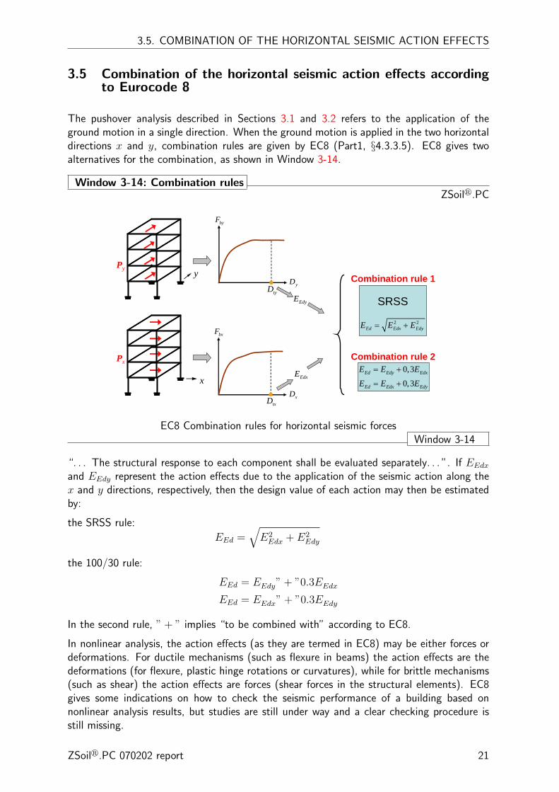
The pushover analysis described in Sections 3.1 and 3.2 refers to the application of theground motion in a single direction. When the ground motion is applied in the two horizontaldirections x and y, combination rules are given by EC8 (Part1, §4.3.3.5). EC8 gives twoalternatives for the combination, as shown in Window 3-14.

Window 3-14: Combination rulesZSoilr.PC

Py

Px

y

x

tyD

byF

yD

bxF

xDtxD

EdyE

EdxE

2 2Ed Edx EdyE E E= +

SRSS

Combination rule 1

Combination rule 20,3

0,3Ed Edy Edx

Ed Edx Edy

E E E

E E E

= +

= +

EC8 Combination rules for horizontal seismic forcesWindow 3-14

“. . . The structural response to each component shall be evaluated separately. . . ”. If EEdxand EEdy represent the action effects due to the application of the seismic action along thex and y directions, respectively, then the design value of each action may then be estimatedby:

the SRSS rule:

EEd =√E2Edx + E2

Edy

the 100/30 rule:

EEd = EEdy” + ”0.3EEdx

EEd = EEdx” + ”0.3EEdy

In the second rule, ” + ” implies “to be combined with” according to EC8.

In nonlinear analysis, the action effects (as they are termed in EC8) may be either forces ordeformations. For ductile mechanisms (such as flexure in beams) the action effects are thedeformations (for flexure, plastic hinge rotations or curvatures), while for brittle mechanisms(such as shear) the action effects are forces (shear forces in the structural elements). EC8gives some indications on how to check the seismic performance of a building based onnonlinear analysis results, but studies are still under way and a clear checking procedure isstill missing.


Chapter 4

NONLINEAR MODELING INEUROCODE 8

EC8 does not give any specific guidelines on how to consider material nonlinarities. Onlygeneral statements are made in EC8 Part 1 §4.3.3.4.1. The model shall include the strengthof structural elements and their post-elastic behaviour. As a minimum, a bilinear force-deformation relationship should be used at the element level. For bilinear force-deformationrelationship (typical of ductile mechanisms such as the bending moment – curvature in re-inforced concrete beams) the elastic stiffness should be that of the cracked section and canbe computed as the secant stiffness to the yield point. Zero post-yield stiffness may be as-sumed. Strength degradation may be included using more refined constitutive laws. Theseare minimum requirements for basic constitutive laws. For a fiber section model, for example,the section behaviour derives from the fibers’ behaviour. Element properties should be basedon mean values of the material properties. For new structures, mean values of the materialproperties may be estimated from the corresponding characteristic values on the basis ofspecific Eurocodes (for example EC2 for concrete).

EC8 Part 1 §4.4.2.2, which deals with resistance conditions at the Ultimate Limit State,provides guidelines on geometric nonlinearities. Second-order, or P-D effects, need not betaken into account if the following condition is satisfied:

θ =PtotdrVtoth

≤ 0.10

where θ is the interstorey drift sensitivity coefficient, Ptot is the total gravity load at and abovethe storey considered in the seismic design situation, dr is the design interstorey drift, evalu-ated as the average lateral displacement ds at the bottom of the storey under considerationand calculated in accordance with EC8 Part 1 §4.3.4, Vtot is the total seismic storey shear,h is the interstorey height. If 0.1 < θ ≤ 0.20 the second order effects may approximatelybe taken into account by multiplying the relevant seismic action effects by a factor equal to1/(1−θ). Finally, the value of the interstorey drift sensitivity coefficient is limited by θ = 0.3.

The above conditions relate to the ultimate limit state. It appears that these rules ap-ply mainly to linear methods of analysis. For nonlinear analysis, no specifics are given ongeometric nonlinearities and the published literature lacks studies on the importance of ac-counting for geometric nonlinearities in either pushover or time-history analyses. From limitedpublished data and common experience it appears that for more flexible buildings in zones ofhigh seismicity, geometric nonlinearities will have an important effect on the overall response

CHAPTER 4. NONLINEAR MODELING IN EUROCODE 8

at the ultimate limite state. For analyses at the collapse limit state, geometric nonlinearitiesshould always be considered.


Chapter 5

Applications: Study of Bonefro buidling

The study of the seismic response of an existing reinforced concrete building which is analyzedusing both nonlinear pushover and time history analyses results according to EC8 is presented.

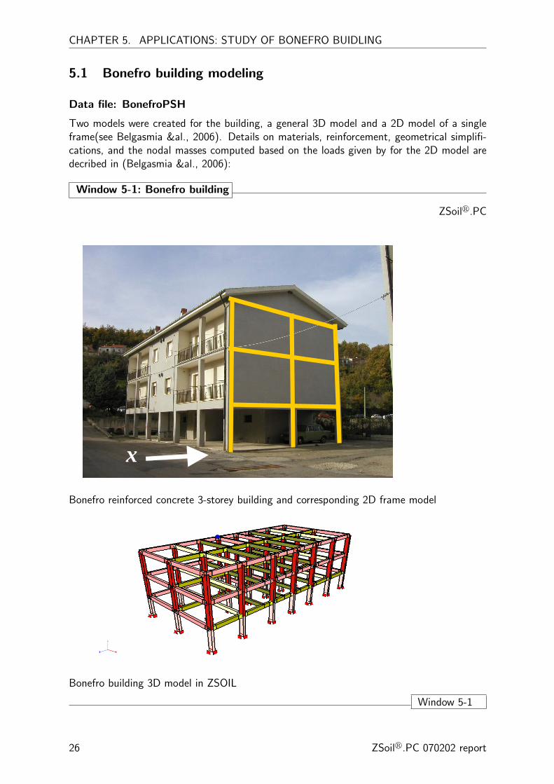
An existing three-storey reinforced concrete building is studied using the nonlinear frameanalysis capabilities of ZSoilr. The building is in Bonefro, Italy, and is a good example ofresidential buildings of the 70’s and 80’s in Italy, prior to the introduction of the seismic codein the early 80’s.

CHAPTER 5. APPLICATIONS: STUDY OF BONEFRO BUIDLING

5.1 Bonefro building modeling

Data file: BonefroPSH

Two models were created for the building, a general 3D model and a 2D model of a singleframe(see Belgasmia &al., 2006). Details on materials, reinforcement, geometrical simplifi-cations, and the nodal masses computed based on the loads given by for the 2D model aredecribed in (Belgasmia &al., 2006):

Window 5-1: Bonefro building

ZSoilr.PC

x

Bonefro reinforced concrete 3-storey building and corresponding 2D frame model

1P

Bonefro building 3D model in ZSOIL

Window 5-1


5.2 RESPONSE OF BONEFRO BUILDING TO 2D PUSHOVER ANALYSIS

5.2 Response of Bonefro building to ground acceleration, compari-son of force and displacement based elements

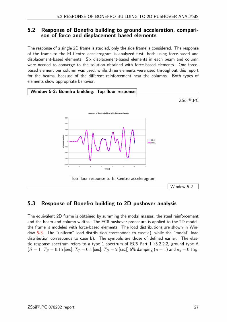
The response of a single 2D frame is studied, only the side frame is considered. The responseof the frame to the El Centro accelerogram is analyzed first, both using force-based anddisplacement-based elements. Six displacement-based elements in each beam and columnwere needed to converge to the solution obtained with force-based elements. One force-based element per column was used, while three elements were used throughout this reportfor the beams, because of the different reinforcement near the columns. Both types ofelements show appropriate behavior.

Window 5-2: Bonefro building: Top floor response

ZSoilr.PC

response of Bonefro building to EL Centro earthquake

-0.08

-0.06

-0.04

-0.02

0

0.02

0.04

0.06

0.08

0 1 2 3 4 5 6 7

time(s)

disp

lace

men

t(m

)

DB d3FB d3

Top floor response to El Centro accelerogram

Window 5-2

5.3 Response of Bonefro building to 2D pushover analysis

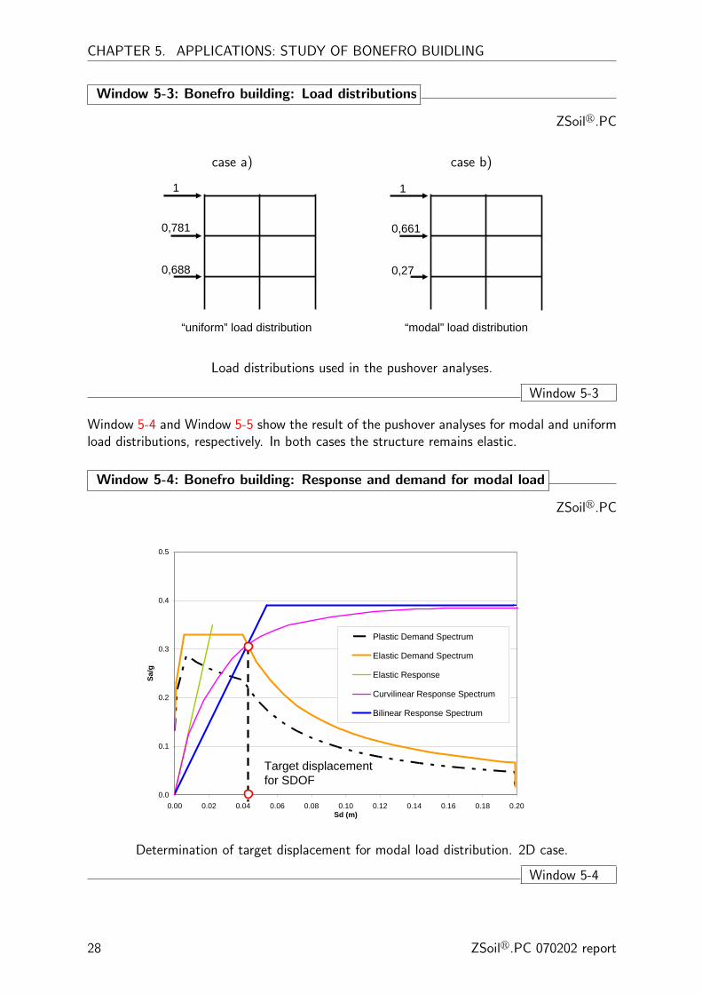
The equivalent 2D frame is obtained by summing the modal masses, the steel reinforcementand the beam and column widths. The EC8 pushover procedure is applied to the 2D model,the frame is modeled with force-based elements. The load distributions are shown in Win-dow 5-3. The “uniform” load distribution corresponds to case a), while the “modal” loaddistribution corresponds to case b). The symbols are those of defined earlier. The elas-tic response spectrum refers to a type 1 spectrum of EC8 Part 1 §3.2.2.2, ground type A(S = 1, TB = 0.15 [sec], TC = 0.4 [sec], TD = 2 [sec]) 5% damping (η = 1) and ag = 0.15g.



Window 5-3: Bonefro building: Load distributions

ZSoilr.PC

case a) case b)

1

0,781

0,688

1

0,661

0,27

“uniform” load distribution “modal” load distribution

Load distributions used in the pushover analyses.

Window 5-3

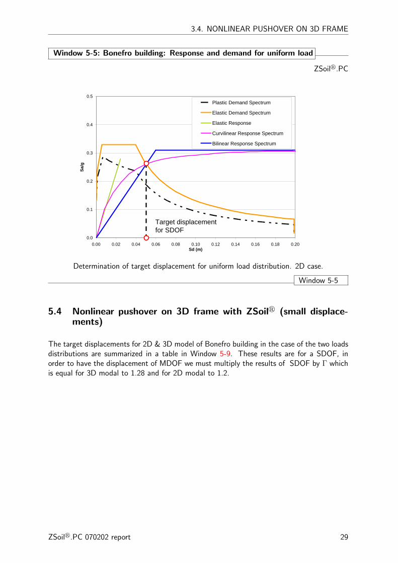
Window 5-4 and Window 5-5 show the result of the pushover analyses for modal and uniformload distributions, respectively. In both cases the structure remains elastic.

Window 5-4: Bonefro building: Response and demand for modal load

ZSoilr.PC

0.0

0.1

0.2

0.3

0.4

0.5

0.00 0.02 0.04 0.06 0.08 0.10 0.12 0.14 0.16 0.18 0.20Sd (m)

Sa/g

Plastic Demand Spectrum

Elastic Demand Spectrum

Elastic Response

Curvilinear Response Spectrum

Bilinear Response Spectrum

Target displacement for SDOF

Determination of target displacement for modal load distribution. 2D case.

Window 5-4


3.4. NONLINEAR PUSHOVER ON 3D FRAME

Window 5-5: Bonefro building: Response and demand for uniform load

ZSoilr.PC

0.0

0.1

0.2

0.3

0.4

0.5

0.00 0.02 0.04 0.06 0.08 0.10 0.12 0.14 0.16 0.18 0.20Sd (m)

Sa/g



Elastic Response




Determination of target displacement for uniform load distribution. 2D case.

Window 5-5

5.4 Nonlinear pushover on 3D frame with ZSoilr (small displace-ments)

The target displacements for 2D & 3D model of Bonefro building in the case of the two loadsdistributions are summarized in a table in Window 5-9. These results are for a SDOF, inorder to have the displacement of MDOF we must multiply the results of SDOF by Γ whichis equal for 3D modal to 1.28 and for 2D modal to 1.2.



Window 5-6: Bonefro building (3D): Response and demand for modal load

ZSoilr.PC

0.0

0.1

0.2

0.3

0.4

0.5

0.00 0.02 0.04 0.06 0.08 0.10 0.12 0.14 0.16 0.18 0.20Sd (m)

Sa/g



Elastic Response




Determination of target displacement for modal loading in x direction.

Window 5-6

Window 5-7: Bonefro building (3D): Response and demand for uniform load)

ZSoilr.PC

0.0

0.1

0.2

0.3

0.4

0.5

0.00 0.02 0.04 0.06 0.08 0.10 0.12 0.14 0.16 0.18 0.20Sd (m)

Sa/g



Elastic Response




Determination of target displacement for uniform load distribution.

Window 5-7


5.5. SIMULATED ACCELEROGRAMS

Window 5-8: Bonefro building: Pushover curves (3D and 2D)

ZSoilr.PC

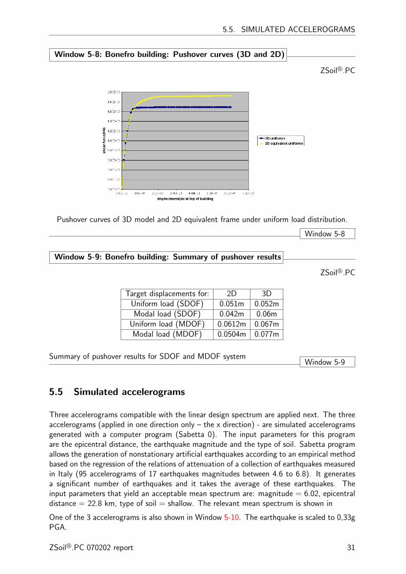
Pushover curves of 3D model and 2D equivalent frame under uniform load distribution.

Window 5-8

Window 5-9: Bonefro building: Summary of pushover results

ZSoilr.PC

Target displacements for: 2D 3DUniform load (SDOF) 0.051m 0.052mModal load (SDOF) 0.042m 0.06m

Uniform load (MDOF) 0.0612m 0.067mModal load (MDOF) 0.0504m 0.077m

Summary of pushover results for SDOF and MDOF systemWindow 5-9

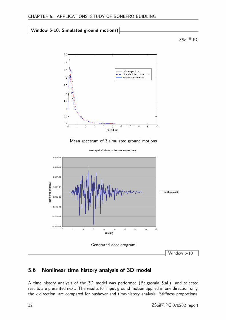
5.5 Simulated accelerograms

Three accelerograms compatible with the linear design spectrum are applied next. The threeaccelerograms (applied in one direction only – the x direction) - are simulated accelerogramsgenerated with a computer program (Sabetta 0). The input parameters for this programare the epicentral distance, the earthquake magnitude and the type of soil. Sabetta programallows the generation of nonstationary artificial earthquakes according to an empirical methodbased on the regression of the relations of attenuation of a collection of earthquakes measuredin Italy (95 accelerograms of 17 earthquakes magnitudes between 4.6 to 6.8). It generatesa significant number of earthquakes and it takes the average of these earthquakes. Theinput parameters that yield an acceptable mean spectrum are: magnitude = 6.02, epicentraldistance = 22.8 km, type of soil = shallow. The relevant mean spectrum is shown in

One of the 3 accelerograms is also shown in Window 5-10. The earthquake is scaled to 0,33gPGA.



Window 5-10: Simulated ground motions)

ZSoilr.PC

Mean spectrum of 3 simulated ground motions

earthquake3 close to Eurocode spectrum

-3.50E-01

-2.50E-01

-1.50E-01

-5.00E-02

5.00E-02

1.50E-01

2.50E-01

3.50E-01

0 2 4 6 8 10 12 14 16 18

time(s)

acce

lera

tion(

m/s

2)

earthquake3

Generated accelerogram

Window 5-10

5.6 Nonlinear time history analysis of 3D model

A time history analysis of the 3D model was performed (Belgasmia &al.) and selectedresults are presented next. The results for input ground motion applied in one direction only,the x direction, are compared for pushover and time-history analysis. Stiffness proportional


5.7. SENSITIVITY TO SEISMIC PARAMETERS

Rayleigh damping is prescribed, with 5% damping at 2 Hertz. The resulting values for Rayleighdamping are α = 0 and β = 0.008. The top-floor response to the selected accelerogramis shown in Window 5-11, representing the maximum response out of 3 acceleration time-histories, as prescribed by EC8.

The maximum top floor displacement for the three earthquakes is 0.072 [m]. The targetdisplacement for the pushover analysis is 0.077 [m].

Window 5-11: Response to simulated ground motions)

ZSoilr.PC

Ux0.1

-0.1

0.0

Top floor response of 3D building to earthquake 3

Window 5-11

Pushover analysis provides the maximum base shear one can expect for a given maximumtarget displacement (corresponding to a given earthquake intensity). The time historiesprovide not only the maximum values, but the entire history. For the example at hand, themax displacement of the time history is 0.072m, and the maximum base shear is approximatelyequal to 1500 kN, but during the time history this value of the base shear can be reachedat several instances and for different values of the top displacement. On the pushover curvethis translates into a single point that provides maximum displacement and maximum baseshear that can be expected for that given earthquake.

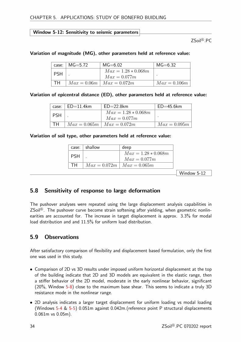
5.7 Sensitivity to seismic parameters

The sensitivity of the time history analyses to the seismic parameters used in generatingthe accelerograms with the program Sabetta 0 is presented here. The three parameters:magnitude, epicenter distance and soil type were varied. The results are shown in the followingtables. The reference values are magnitude MG= 6.02, epicenter distance ED = 22.8 km,shallow soil type. Following tables gives maximum displacement response under:

• modal load in x direction for static pushover analysis (PSH)

• earthquakes in x direction for Time history analysis (TH)



Window 5-12: Sensitivity to seismic parameters

ZSoilr.PC

Variation of magnitude (MG), other parameters held at reference value:

case: MG=5.72 MG=6.02 MG=6.32

PSH .Max = 1.28 ∗ 0.068mMax = 0.077m

.

TH Max = 0.06m Max = 0.072m Max = 0.106m

Variation of epicentral distance (ED), other parameters held at reference value:

case: ED=11.4km ED=22.8km ED=45.6km

PSH .Max = 1.28 ∗ 0.068mMax = 0.077m

.

TH Max = 0.065m Max = 0.072m Max = 0.095m

Variation of soil type, other parameters held at reference value:

case: shallow deep

PSH .Max = 1.28 ∗ 0.068mMax = 0.077m

TH Max = 0.072m Max = 0.065m

Window 5-12

5.8 Sensitivity of response to large deformation

The pushover analyses were repeated using the large displacement analysis capabilities inZSoilr. The pushover curve become strain softening after yielding, when geometric nonlin-earities are accounted for. The increase in target displacement is approx. 3.3% for modalload distribution and and 11.5% for uniform load distribution.

5.9 Observations

After satisfactory comparison of flexibility and displacement based formulation, only the firstone was used in this study.

• Comparison of 2D vs 3D results under imposed uniform horizontal displacement at the topof the building indicate that 2D and 3D models are equivalent in the elastic range, thena stiffer behavior of the 2D model, moderate in the early nonlinear behavior, significant(20%, Window 5-8) close to the maximum base shear. This seems to indicate a truly 3Dresistance mode in the nonlinear range.

• 2D analysis indicates a larger target displacement for uniform loading vs modal loading(Windows 5-4 & 5-5) 0.051m against 0.042m.(reference point P structural displacements0.061m vs 0.05m).


5.9. OBSERVATIONS

• 3D analysis, uniform loading vs modal loading, indicates the opposite trend, (Windows 5-6& 5-7), 0.052m against 0.06m. (at P 0.067m vs 0.077m)

• Combining loading, 100% in x direction and 30% in z direction shows no influence on thepushover curve and hence on the target displacement.

• The comparison between pushover and dynamics gives a difference of 7% (dmax modalfrom pushover/ dmax dynamics) =0.077/0.072.

• The sensitivity to Magnitude, in dynamics a (+-5%) variation in EQ magnitude yields avariation in max displacement of ( +47% and –17%).

• The sensitivity to epicenter distance, in dynamics (via Sabetta program) a (+100%, -50%)variation yields a variation in max displacement of (+31%, -10%).

• The sensitivity to soil, in dynamics (via Sabetta program): shallow/deep = 0.072/0.065=1.1the difference is about 10%.

• The maximum base shear indicated by the pushover analysis is systematically reachedfor almost any maximum top displacement during dynamic, this is probably indicative ofsignificant influence of 2nd 3rd etc modes.

• Large displacement induce global softening and increase target displacements in 3D pushover+11% for uniform loading 0.058/0.052, +3% for modal loading 0.062/0.06. No influencewas noticed in dynamics.


Chapter 6

Data preparation for pushover analysisin ZSoilr.PC

Data preparation for pushover analysis requires specification of the following data:

• Control phase:

F Activating driver(s)under Menu/Control/Analysis and drivers

F Setting control data for each driver under Menu/Control/Pushover

• Preprocessing phase:

F Introducing masses to the FE model of the structure. See Section 6.2

F Selecting and labeling control node i.e. node where target displacement is set. SeeSection 6.3

The example (file xFrame3D.inp) concerns a simple reinforced concrete 3D frame repre-senting the skeleton of a two-storey building (with stiffness of the wall neglected).

The structure is shown in the Window 6-1

CHAPTER 6. DATA PREPARATION FOR PUSHOVER ANALYSIS IN ZSOILr.PC

Window 6-1: Example of FE model)

ZSoilr.PC

6.0

6.0

6.0

4.0

4.0

p2 =20kN/m

p1 =30kN/m

Control node

M1 = 12000kg

M1

M1M1

M2=18000kg

M2

M2

M2

M2

M2M3

M3=27000kg

12Ø25XZ

xFrame3D FE model. Masses, loads and control node

Window 6-1

For sake of presentation simplicity there is one reinforced concrete section assumed in allmembers with dimension 0.4 × 0.3m, made of concrete characterized by fc = 25MPa,ft = 1.8MPa, reinforced by symmetric reinforcement 10∅25 as shown.

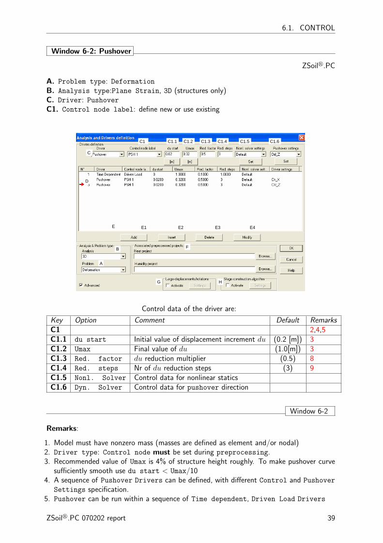
6.1 Control

Pushover analysis is a ZSoilr driver activated under Control / Analysis & Drivers.Pushover should be run after evaluation of the mechanical state of the structure correspond-ing to gravity load in a sequence of Initial State and/or Time dependent, Driven Load

Drivers.


6.1. CONTROL

Window 6-2: Pushover

ZSoilr.PC

A. Problem type: Deformation

B. Analysis type:Plane Strain, 3D (structures only)C. Driver: Pushover

C1. Control node label: define new or use existing

A

B

C

D

E

F

C1 C1.1 C1.2 C1.3 C1.4

E1 E2 E3 E4

C1.5

G H

C1.6

Control data of the driver are:

Key Option Comment Default RemarksC1 2,4,5C1.1 du start Initial value of displacement increment du (0.2 [m]) 3C1.2 Umax Final value of du (1.0[m]) 3C1.3 Red. factor du reduction multiplier (0.5) 8C1.4 Red. steps Nr of du reduction steps (3) 9C1.5 Nonl. Solver Control data for nonlinear staticsC1.6 Dyn. Solver Control data for pushover direction

Window 6-2

Remarks:

1. Model must have nonzero mass (masses are defined as element and/or nodal)2. Driver type: Control node must be set during preprocessing.3. Recommended value of Umax is 4% of structure height roughly. To make pushover curve

sufficiently smooth use du start < Umax/104. A sequence of Pushover Drivers can be defined, with different Control and Pushover

Settings specification.5. Pushover can be run within a sequence of Time dependent, Driven Load Drivers



6. The state of the structure at start of a pushover driver takes into account results (e.g.plastic status, stresses, deformation) ) of previous Time dependent driver(s).

7. Changes of the structure state (stresses, deformation, plastic status) induced by pushover

driver are disregarded during subsequent drivers of any type8. Step reduction procedure is automatically performed in case when applying initially set du

causes divergence.9. When convergence is not reached after applying displacement increment reduced Red.

steps times from its initial value du, execution of the static procedure is terminatedbefore reaching final value Umax.

10. Large deformation analysis may be activated.11. After running pushover driver use Postprocessing/Pushover Result to perform seis-

mic demand assessment automatically.

Other data to be defined are:

• Nonlinear solver settings (use Control / Control)The only data taken into account during pushover analysis are:

F Tolerance for solid phase RHSF Absolute max. nr of iterations -if reached, the step length reduction is performed

• Pushover settings: (use Control / Pushover)

F Label can be given to ease identification of the given set in case of multiple use in onejob,

F Mass filtering (if on) will be performed in specified direction

F Direction - the vector introduced will be used to set: pushover force direction, controldisplacement direction, and mass filtering (if activated),

F Force pattern- selection between Modal, Uniform or Triangular, see Window 3-1

6.2 Modeling of masses

ZSoilr offers different possibilities to model masses present in the structure. They include:

• Element massesThey are related to the material density and geometry of the structural element itself. Ineach element type they have to be defined as a part of material model attached to theelement. Their existence at a given instant of the analysis is controlled by the elementitself.• Added masses

They can be added independently from element description, their activity (existence) canbe controlled by existence and load functions. They can be attached to:

F a node (by specifying total nodal mass),F an edge or existing beam and truss (by specifying linear mass density),F a face of a shell (by specifying surface mass density).

In ZSoilr 2011 lumped (diagonal) or consistent mass matrix is created in each of the abovecases.


6.3. SELECTION OF A CONTROL NODE

In the example xFrame3D there are element masses originating from the element deadweight set during material (i.e. cross-section properties) definition, see the figure as well asnodal masses (due to mass of walls and floors other than mass of frame member itself)attached to each node of the 1-st and 2-nf floor set during Prepro set under FE model /Added masses / Nodal mass.

Window 6-3: Element masses

ZSoilr.PC

Setting element masses

Window 6-3

6.3 Selection of a control node

If pushover analysis is to be run, a control node must be selected (in interactive graphicalmanner) during pre-processing phase. This must be done prior to activation of PushoverDrivers from the Menu/Control /Analysis & Drivers. The node should be labeled.

In the example xFrame3D there is one control node set under Prepro option Domain/Pushovercontrol node, labeled as PSH 1, see the figure.

6.4 Results

Section describe actions specific to pushover result handling. These include:

• Automated seismic demand assessment under Menu/Results/Pushover results, see Section6.5• Tracing structural performance under graphical postprocessor under

Menu/Results/Postprocessing, see Section 6.6.



6.5 Pushover results

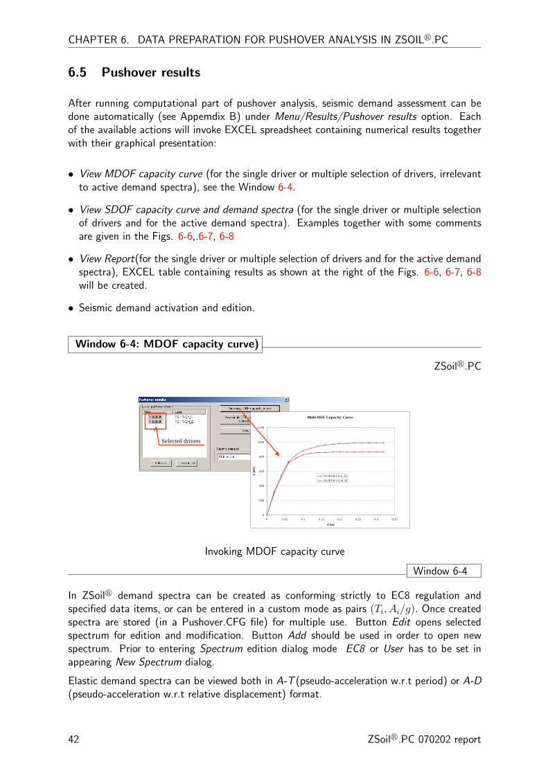
After running computational part of pushover analysis, seismic demand assessment can bedone automatically (see Appemdix B) under Menu/Results/Pushover results option. Eachof the available actions will invoke EXCEL spreadsheet containing numerical results togetherwith their graphical presentation:

• View MDOF capacity curve (for the single driver or multiple selection of drivers, irrelevantto active demand spectra), see the Window 6-4.

• View SDOF capacity curve and demand spectra (for the single driver or multiple selectionof drivers and for the active demand spectra). Examples together with some commentsare given in the Figs. 6-6,.6-7, 6-8

• View Report(for the single driver or multiple selection of drivers and for the active demandspectra), EXCEL table containing results as shown at the right of the Figs. 6-6, 6-7, 6-8will be created.

• Seismic demand activation and edition.

Window 6-4: MDOF capacity curve)

ZSoilr.PC

Multi DOF Capacity Curve

0

200

400

600

800

1000

1200

0 0.05 0.1 0.15 0.2 0.25 0.3 0.35

d [m]

V [k

N]

Vb (P S H 1/Ctr_X)Vb (P S H 1/Ctrl_Z)

Selected drivers

Invoking MDOF capacity curve

Window 6-4

In ZSoilr demand spectra can be created as conforming strictly to EC8 regulation andspecified data items, or can be entered in a custom mode as pairs (Ti, Ai/g). Once createdspectra are stored (in a Pushover.CFG file) for multiple use. Button Edit opens selectedspectrum for edition and modification. Button Add should be used in order to open newspectrum. Prior to entering Spectrum edition dialog mode EC8 or User has to be set inappearing New Spectrum dialog.

Elastic demand spectra can be viewed both in A-T (pseudo-acceleration w.r.t period) or A-D(pseudo-acceleration w.r.t relative displacement) format.


6.5. PUSHOVER RESULTS

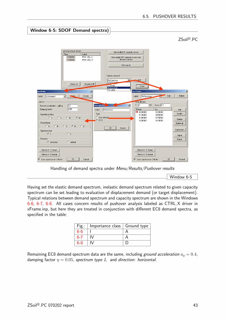
Window 6-5: SDOF Demand spectra)

ZSoilr.PC

Handling of demand spectra under Menu/Results/Pushover results

Window 6-5

Having set the elastic demand spectrum, inelastic demand spectrum related to given capacityspectrum can be set leading to evaluation of displacement demand (or target displacement).Typical relations between demand spectrum and capacity spectrum are shown in the Windows6-6, 6-7, 6-8. All cases concern results of pushover analysis labeled as CTRL X driver inxFrame.inp, but here they are treated in conjunction with different EC8 demand spectra, asspecified in the table:

Fig.: Importance class Ground type6-6 I A6-7 IV A6-8 IV D

Remaining EC8 demand spectrum data are the same, including ground acceleration ag = 0.4,damping factor η = 0.05, spectrum type 1, and direction: horizontal.



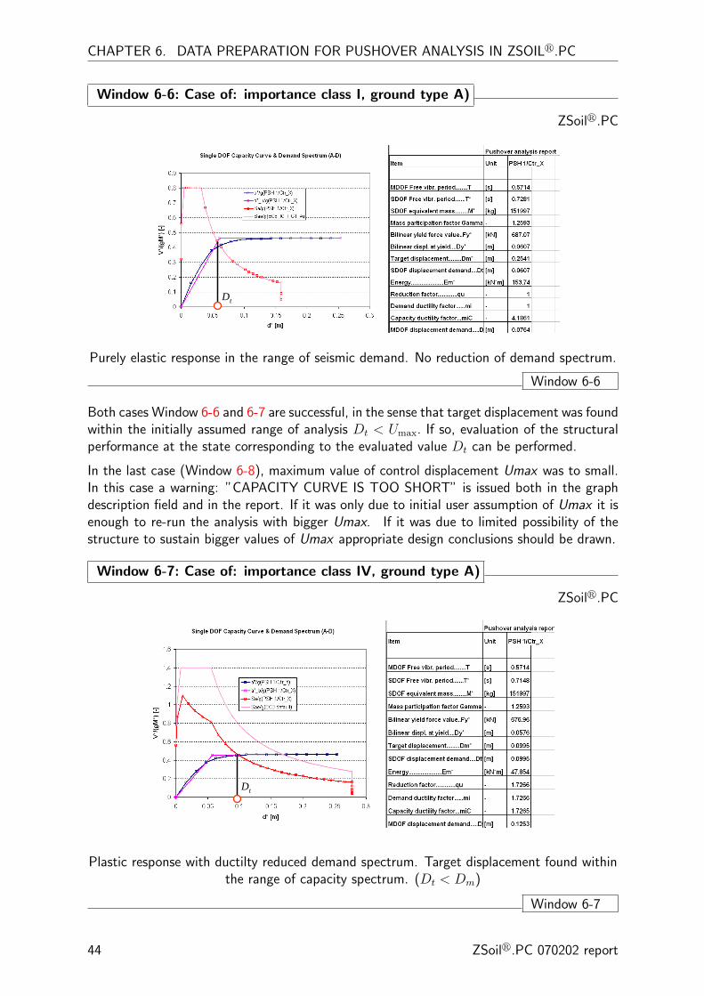
Window 6-6: Case of: importance class I, ground type A)

ZSoilr.PC

Dt

Purely elastic response in the range of seismic demand. No reduction of demand spectrum.

Window 6-6

Both cases Window 6-6 and 6-7 are successful, in the sense that target displacement was foundwithin the initially assumed range of analysis Dt < Umax. If so, evaluation of the structuralperformance at the state corresponding to the evaluated value Dt can be performed.

In the last case (Window 6-8), maximum value of control displacement Umax was to small.In this case a warning: ”CAPACITY CURVE IS TOO SHORT” is issued both in the graphdescription field and in the report. If it was only due to initial user assumption of Umax it isenough to re-run the analysis with bigger Umax. If it was due to limited possibility of thestructure to sustain bigger values of Umax appropriate design conclusions should be drawn.

Window 6-7: Case of: importance class IV, ground type A)

ZSoilr.PC

Dt

Plastic response with ductilty reduced demand spectrum. Target displacement found withinthe range of capacity spectrum. (Dt < Dm)

Window 6-7


6.6. POSTPROCESSING

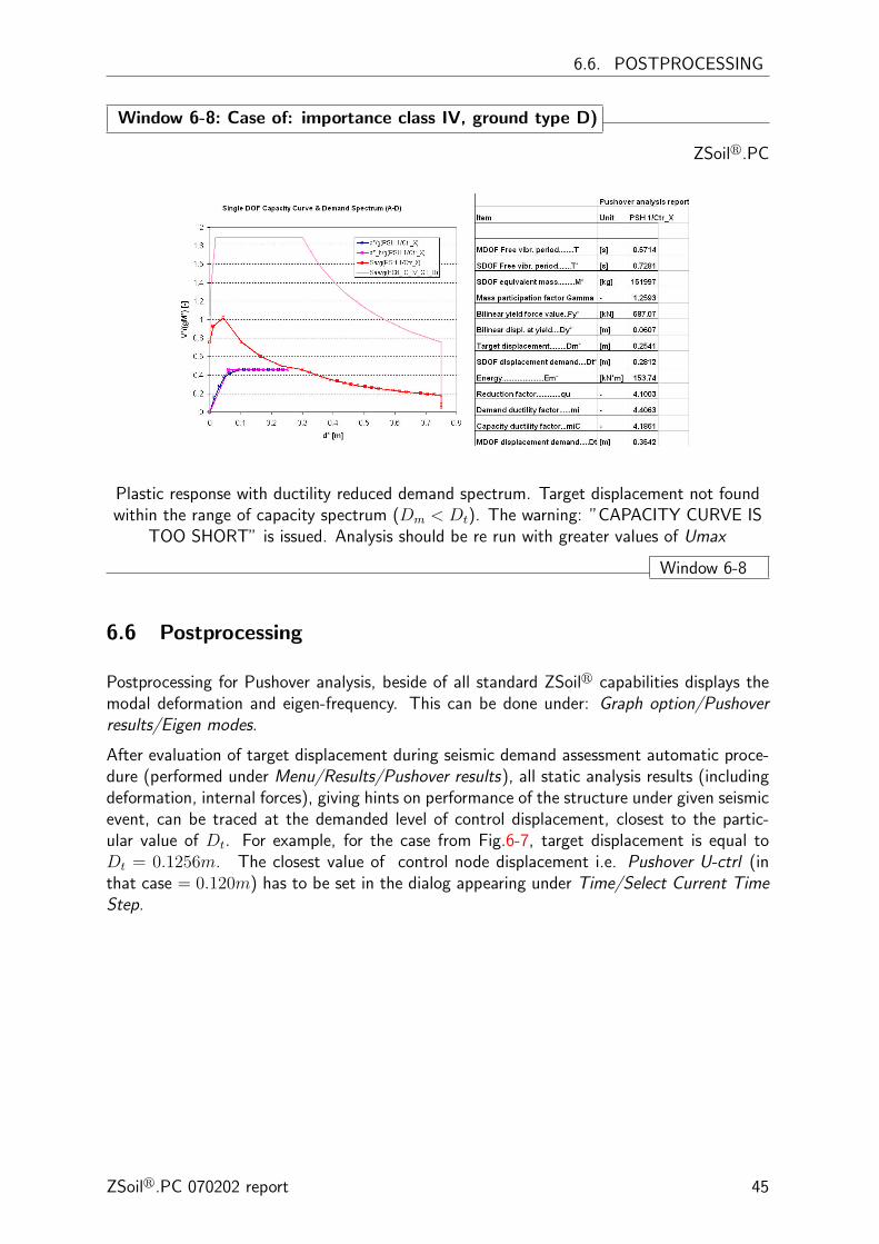
Window 6-8: Case of: importance class IV, ground type D)

ZSoilr.PC

Plastic response with ductility reduced demand spectrum. Target displacement not foundwithin the range of capacity spectrum (Dm < Dt). The warning: ”CAPACITY CURVE IS

TOO SHORT” is issued. Analysis should be re run with greater values of Umax

Window 6-8

6.6 Postprocessing

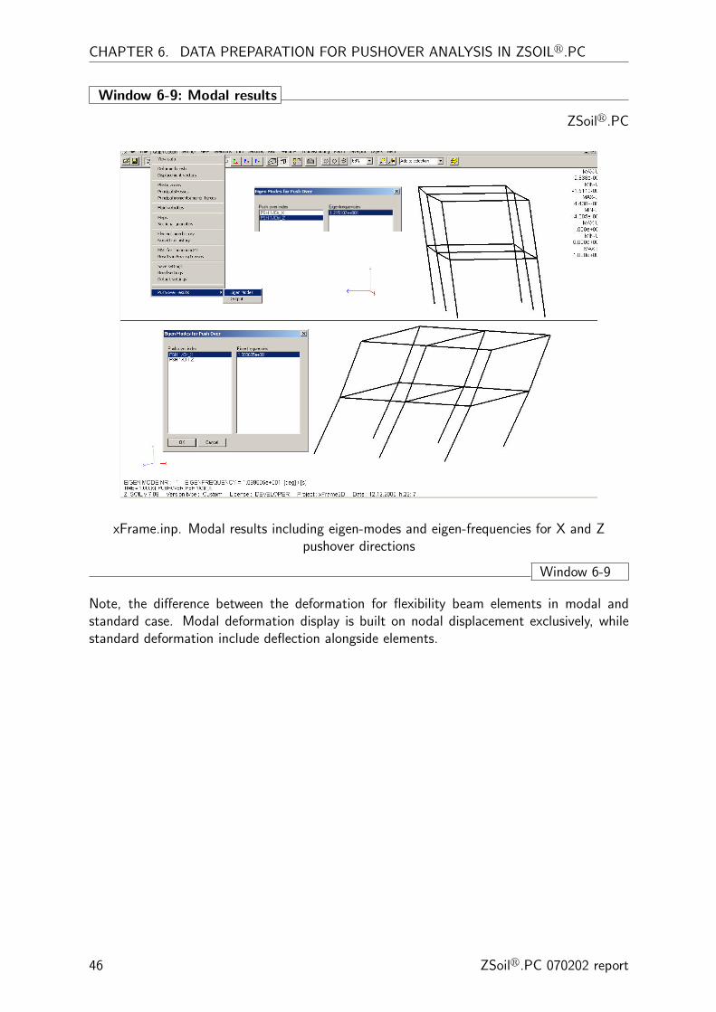
Postprocessing for Pushover analysis, beside of all standard ZSoilr capabilities displays themodal deformation and eigen-frequency. This can be done under: Graph option/Pushoverresults/Eigen modes.

After evaluation of target displacement during seismic demand assessment automatic proce-dure (performed under Menu/Results/Pushover results), all static analysis results (includingdeformation, internal forces), giving hints on performance of the structure under given seismicevent, can be traced at the demanded level of control displacement, closest to the partic-ular value of Dt. For example, for the case from Fig.6-7, target displacement is equal toDt = 0.1256m. The closest value of control node displacement i.e. Pushover U-ctrl (inthat case = 0.120m) has to be set in the dialog appearing under Time/Select Current TimeStep.



Window 6-9: Modal results

ZSoilr.PC

xFrame.inp. Modal results including eigen-modes and eigen-frequencies for X and Zpushover directions

Window 6-9

Note, the difference between the deformation for flexibility beam elements in modal andstandard case. Modal deformation display is built on nodal displacement exclusively, whilestandard deformation include deflection alongside elements.


6.6. POSTPROCESSING

Window 6-10: Static results

ZSoilr.PC

xFrame.inp. Static results including deformation and bending moments for X-direction adUctrl = 0.12 [m]

Window 6-10



References

1. S. Antoniou and R. Pinho, “Advantages and Limitations of Adaptive and Non-adaptiveForce-Based Pushover Procedures”, Journal of Earthquake Engineering, Vol. 8, No. 4(2004) 497-522.

2. M.N. Aydinoglu, “An Incremental Response Spectrum Analysis Procedure Based on In-elastic Spectral Deformation for Multi-Mode Seismic Performance Evaluation”, Bulletin ofEarthquake Engineering, 1 (2003), 3-36.

3. M.N. Aydinoglu, “An Improved Pushover Procedure for Engineering Practice: IncrementalResponse Spectrum Analysis (IRSA)” in Performance-based seismic design. Concepts andimplementation, Krawinkler and Fajfar eds., Bled, Slovenia, June 28 – July 1, PEER report2004/05, 345-356.

4. M.Belgasmia, E. Spacone, A.Urbanski, Th. Zimmermann. ”Seismic Evaluation of Con-structions: Static Pushover procedure and time history analysis for Nonlinear Frames”,LSC Internal Report, August 2006.

5. J.M. Biggs, “Introduction in structural dynamics.”1964.

6. A.K. Chopra, “Dynamics of Structures: Theory and Applications to Earthquake Engineer-ing” 2nd Ed., Prentice Hall, Upper Saddle River, NJ, 2001.

7. A.K. Chopra, R.K. Goel, “A modal pushover analysis procedure for estimating seismicdemands for buildings.” Earthquake Engineering and Structural Dynamics 2002, 31:561-582.

8. A.S. Elnashai ”Do we really need Inelastic Dynamic Analysis?” Journal of EarthquakeEngineering, Vol. 6, Special Issue 1 (2002) 123-130.

9. Eurocode 8: Design of Structures for Earthquake Resistance, European Committee forStandardization, 2003.

10. P. Fajfar, “Capacity Spectrum Method Based on Inelastic Demand Spectra.” EarthquakeEngineering and Structural Dynamics, 28. 979-993, 1999.

11. P. Fajfar, “Structural Analysis in Earthquake Engineering – A Breakthrough of SimplifiedNon-Linear Methods.” Proc. 12th European Conference on Earthquake Engineering, Paper843, 2002.

12. P. Fajfar, V. Kilar, D. Marusic, I. Perus, “The extension of the N2 method to asymmet-ric buildings.” Proceedings of the 4th European Workshop on the Seismic Behaviour ofIrregular and Complex Structures, Paper No. 41, Thessaloniki, Greece, 2005.

13. B. Gupta, S.K. Kunnath, “Adaptive Spectra-Based Pushover Procedure for Seismic Eval-uation of Structures”, Earthquake Spectra, 16(2), 367-391.

14. F. Sabetta, A. Pugliese, Estimation of Response Spectra and Simulation of NonstationaryEarthquake Ground Motions, Bulletin of the Seismological Society o America, 86(2) 337-352, 1996.


6.6. POSTPROCESSING

15. E. Spacone, F.C. Filippou, F.F. Taucer, ”Fiber Beam-Column Model for Nonlinear Analysisof R/C Frames. I: Formulation, II: Applications.” Earthquake Engineering and StructuralDynamics, 25(7), 711-742, 1996.

16. T. Vidic, P. Fajfar, M. Fischinger, “Consistent Inelastic Design Spectra: Strength andDisplacement.” Earthquake Engineering and Structural Dynamics, 1994, 23: 502-521.

17. Th. Zimmermann, A. Truty, A. Urbanski, K. Podles. Z-Soil user manual, Zace ServicesLtd, 1985-2006.



Appendix

A1. Seismic demand assesment algorithm

A. Given D∗m, F

∗y from the bilinearized capacity spectrum:

B. Set:

D∗y = 2

(D∗m −

E∗m

F ∗y

); T ∗ = 2π

√m∗D∗

y

F ∗y

; qµ =SAe(T

∗)F ∗y

m∗

C. Reduce spectrum:

if (T ∗ < TC)

qµ ≤ 1⇒ D∗t = SDe(T

∗) response remains elastic

qµ > 1⇒ D∗t =

SDe(T∗)

qµµ; with µ = 1 + (qµ − 1)

TCT ∗

else (T ∗ ≥ TC)

qµ ≤ 1⇒ D∗t = SDe(T

∗) response remains elastic

qµ > 1⇒ D∗t =

SDe(T∗)

qµµ; with µ = q

D. Check:

if |D∗m −D∗

t | < tol stop

else

set : D∗m = D∗

t ,

go to A


6.6. POSTPROCESSING

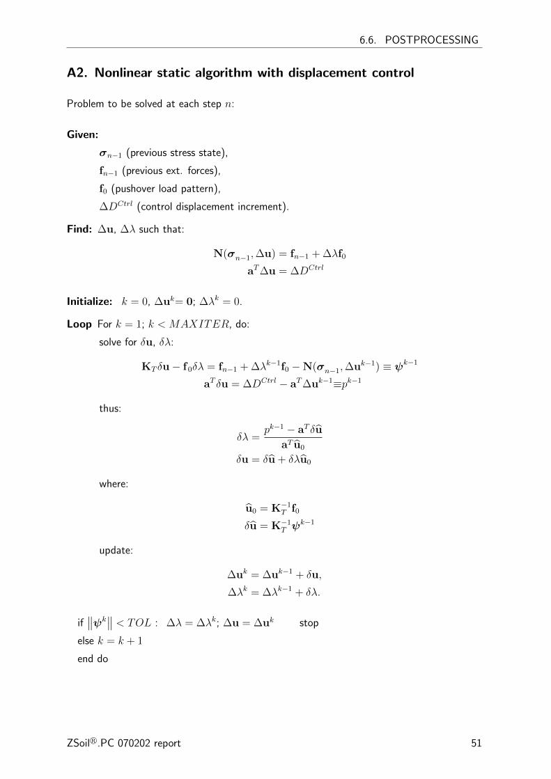
A2. Nonlinear static algorithm with displacement control

Problem to be solved at each step n:

Given:

σn−1 (previous stress state),

fn−1 (previous ext. forces),

f0 (pushover load pattern),

∆DCtrl (control displacement increment).

Find: ∆u, ∆λ such that:

N(σn−1,∆u) = fn−1 + ∆λf0

aT∆u = ∆DCtrl

Initialize: k = 0, ∆uk= 0; ∆λk = 0.

Loop For k = 1; k < MAXITER, do:

solve for δu, δλ:

KT δu− f0δλ = fn−1 + ∆λk−1f0 −N(σn−1,∆uk−1) ≡ ψk−1

aT δu = ∆DCtrl − aT∆uk−1≡pk−1

thus:

δλ =pk−1 − aT δu

aT u0

δu = δu + δλu0

where:

u0 = K−1T f0

δu = K−1T ψ

k−1

update:

∆uk = ∆uk−1 + δu,

∆λk = ∆λk−1 + δλ.

if∥∥ψk

∥∥ < TOL : ∆λ = ∆λk; ∆u = ∆uk stop

else k = k + 1

end do



A3. Step length adjustment algorithm

Step length adjustment algorithm for step n

∆DCtrl = dDCtrl0

for ired = 1; ired < Nred, dogiven: ∆DCtrl, : fn−1, : f0.Solve for: ∆λ, : ∆u, see Appendix A2.if ( converged before MAXITER):

::: fn = fn−1 + ∆λf0, take next step:: n := n+ 1else (diverged after MAXITER ):

::: ∆DCtrl = µ∆DCtrl

if(ired ≤ Nred :: ired := ired+ 1)else Stopend do


STATIC PUSHOVER ANALYSISSTATIC PUSHOVER ANALYSIS ZSoilr.PC 070202 report by A. Urbanski E. Spacone...

Documents

Transcript of STATIC PUSHOVER ANALYSISSTATIC PUSHOVER ANALYSIS ZSoilr.PC 070202 report by A. Urbanski E. Spacone...