Static Program Analysis using

Abstract Interpretation

Introduction

Static Program Analysis

Static program analysis consists of automatically

discovering properties of a program that hold for

all possible execution paths of the program.

Static program analysis is not

• Testing: manually checking a property for

some execution paths

• Model checking: automatically checking a

property for all execution paths

Program Analysis for what?

• Optimizing compilers

• Semantic preprocessing:

– Model checking

– Automated test generation

• Program verification

Program Verification

• Check that every operation of a program

will never cause an error (division by zero,

buffer overrun, deadlock, etc.)

• Example:int a[1000];

for (i = 0; i < 1000; i++)

a[i] = … ; // 0 <= i <= 999

a[i] = … ; // i = 1000;buffer overrun

safe operation

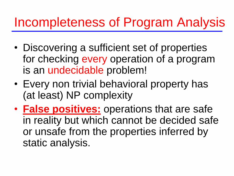
Incompleteness of Program Analysis

• Discovering a sufficient set of properties for checking every operation of a program is an undecidable problem!

• Every non trivial behavioral property has (at least) NP complexity

• False positives: operations that are safe in reality but which cannot be decided safe or unsafe from the properties inferred by static analysis.

Precision versus Efficiency

• Precision and computational complexity

are strongly related

• Tradeoff precision/efficiency: limit in the

average precision and scalability of a

given analyzer

• Greater precision and scalability is

achieved through specialization

Precision: number of program operations that

can be decided safe or unsafe by an analyzer.

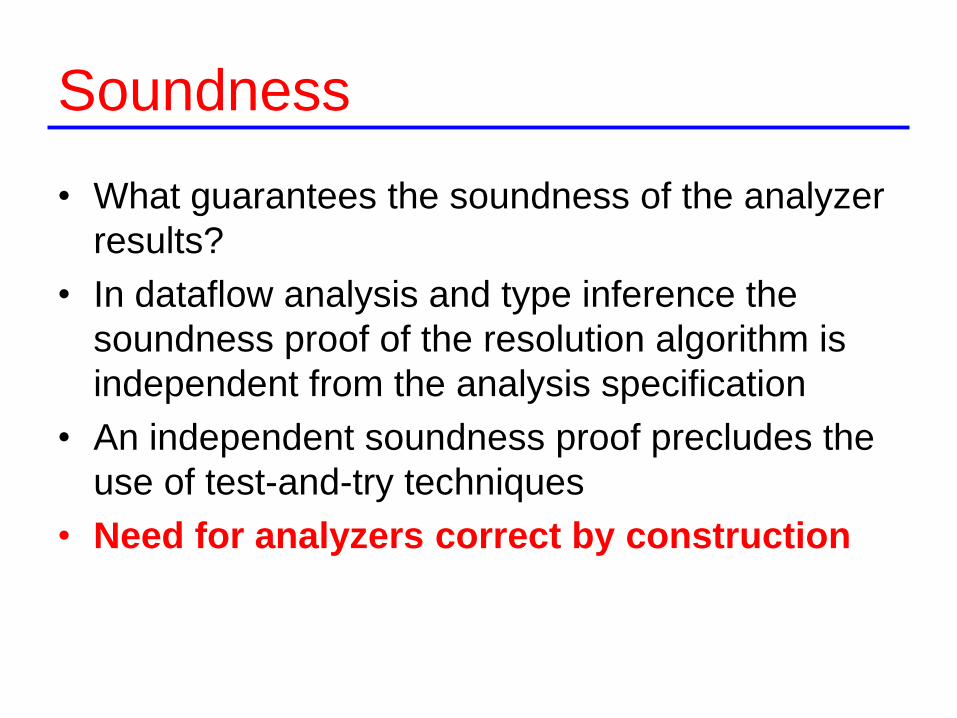
Soundness

• What guarantees the soundness of the analyzer

results?

• In dataflow analysis and type inference the

soundness proof of the resolution algorithm is

independent from the analysis specification

• An independent soundness proof precludes the

use of test-and-try techniques

• Need for analyzers correct by construction

Abstract Interpretation

• A general methodology for designing static

program analyzers that are:

– Correct by construction

– Generic

– Easy to fine-tune

• Scalability is difficult to achieve but the

payoff is worth the effort!

Approximation

• An approximation of memory configurations

is first defined

• Then the approximation of all atomic

operations

• The approximation is automatically lifted to

the whole program structure

The core idea of Abstract Interpretation is the

formalization of the notion of approximation

Overview of Abstract Interpretation

• Start with a formal specification of the program

semantics (the concrete semantics)

• Construct abstract semantic equations w.r.t. a

parametric approximation scheme

• Use general fixpoints algorithms to solve the

abstract semantic equations

• Try-and-test various instantiations of the

approximation scheme in order to find the best fit

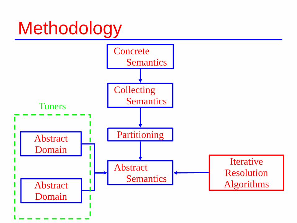
The Methodology of Abstract

Interpretation

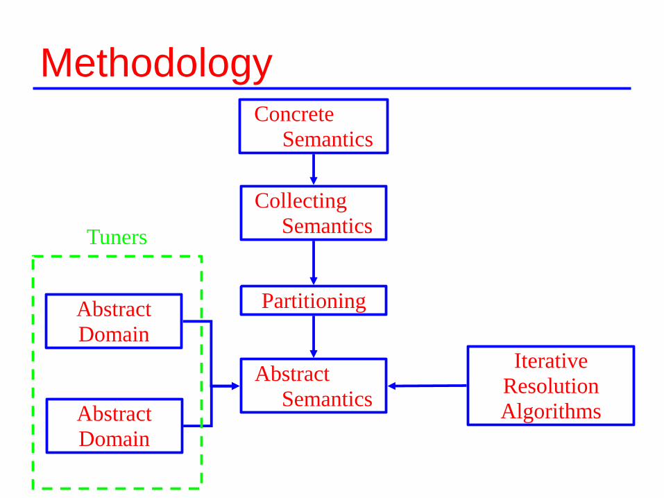
Methodology

Abstract

Semantics

Collecting

Semantics

Partitioning

Concrete

Semantics

Abstract

Domain

Abstract

Domain

Iterative

Resolution

Algorithms

Tuners

Lattices and Fixpoints

• A lattice (L, ⊑, ⊥, ⊔, ⊤, ⊓) is a partially ordered

set (L, ⊑) with:

– Least upper bounds (⊔) and greatest lower

bounds (⊔) operators

– A least element ―bottom‖: ⊥

– A greatest element ―top‖: ⊤

• L is complete if all least upper bounds exist

• A fixpoint X of F: L → L satisfies F(X) = X

• We denote by lfp F the least fixpoint if it exists

Fixpoint Theorems

• Knaster-Tarski theorem: If F: L → L is

monotone and L is a complete lattice, the set of

fixpoints of F is also a complete lattice.

• Kleene theorem: If F: L → L is monotone, L is a

complete lattice and F preserves all least upper

bounds then lfp F is the limit of the sequence:

F0 = ⊥

Fn+1 = F (Fn)

Methodology

Abstract

Semantics

Collecting

Semantics

Partitioning

Concrete

Semantics

Abstract

Domain

Abstract

Domain

Iterative

Resolution

Algorithms

Tuners

Concrete SemanticsSmall-step operational semantics: (

Example:1: n = 0;

2: while n < 1000 do

3: n = n + 1;

4: end

5: exit

1, n n 0 n 0 n 1

n 1 n 1000

s = program point , env s s'

Undefined value

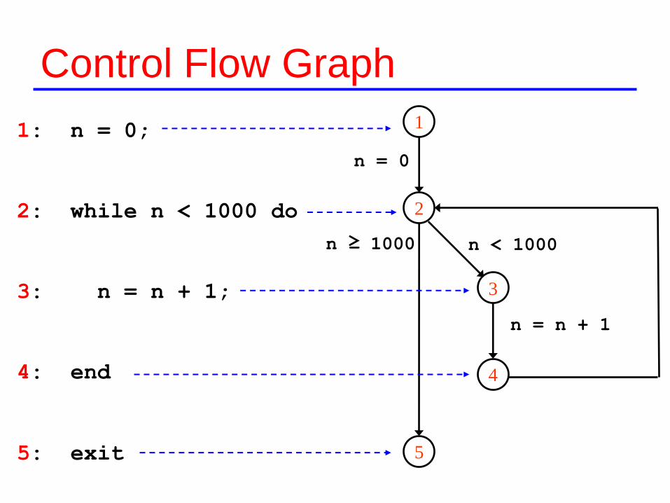
Control Flow Graph

n = 0

n ≥ 1000

1

2

3

4

5

n < 1000

n = n + 1

1: n = 0;

2: while n < 1000 do

3: n = n + 1;

4: end

5: exit

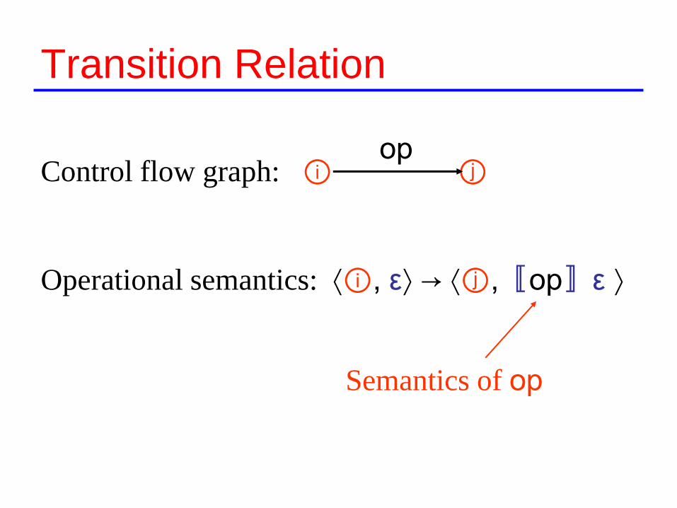
Transition Relation

Control flow graph:

Operational semantics: ⟨, ε⟩ → ⟨,〚op〛ε ⟩

op

Semantics of op

Methodology

Abstract

Semantics

Collecting

Semantics

Partitioning

Concrete

Semantics

Abstract

Domain

Abstract

Domain

Iterative

Resolution

Algorithms

Tuners

Collecting Semantics

• The set of all descendants of the initial state

• The set of all descendants of the initial state that can reach a final state

• The set of all finite traces from the initial state

• The set of all finite and infinite traces from the initial state

• etc.

The collecting semantics is the set of observable behaviours in the operational semantics. It is the starting point of any analysis design.

Which Collecting Semantics?

• Buffer overrun, division by zero, arithmetic

overflows: state properties

• Deadlocks, un-initialized variables: finite

trace properties

• Loop termination: finite and infinite trace

properties

State properties

S = s | s0

s

The set of descendants of the initial state s0:

S = lfp F

F (S) = s0 s' | s S: s s'

Theorem: F : ( ( ), ) ( ( ), )

Example

S = 1, n n 0 n 0 n 1

n 1 n 1000

1: n = 0;

2: while n < 1000 do

3: n = n + 1;

4: end

5: exit

Computation

• F0 = ∅

• F1 = ⟨1,n⇒Ω⟩

• F2 = ⟨1,n⇒Ω⟩, ⟨2,n⇒0⟩

• F3 = ⟨1,n⇒Ω⟩, ⟨2,n⇒0⟩, ⟨3,n⇒0⟩

• F4 = ⟨1,n⇒Ω⟩, ⟨2,n⇒0⟩, ⟨3,n⇒0⟩, ⟨4,n⇒1⟩

• ...

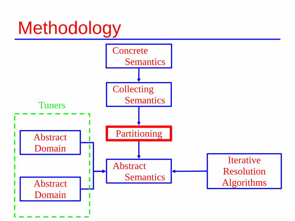
Methodology

Abstract

Semantics

Collecting

Semantics

Partitioning

Concrete

Semantics

Abstract

Domain

Abstract

Domain

Iterative

Resolution

Algorithms

Tuners

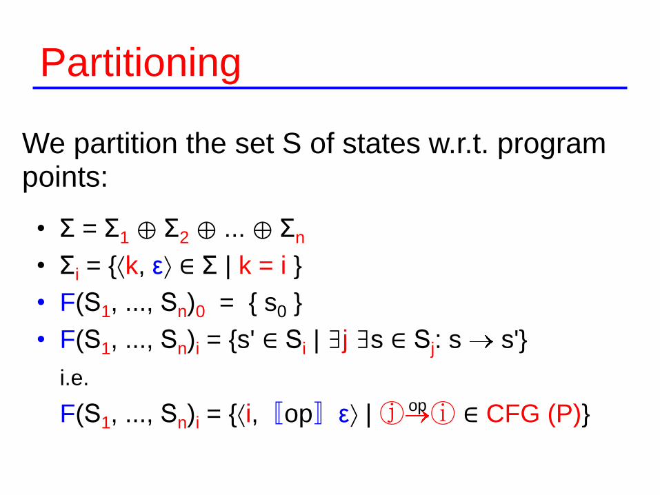
Partitioning

• Σ = Σ1 ⊕ Σ2 ⊕ ... ⊕ Σn

• Σi = ⟨k, ε⟩ ∈ Σ | k = i

• F(S1, ..., Sn)0 = s0

• F(S1, ..., Sn)i = s' ∈ Si | ∃j ∃s ∈ Sj: s s'

i.e.

F(S1, ..., Sn)i = ⟨i,〚op〛ε⟩ | ∈ CFG (P)

We partition the set S of states w.r.t. program points:

op

Illustration

⟨1, e1⟩⟨1, e2⟩

⟨j, ε1⟩

⟨j, ε2⟩

⟨i,〚op〛ε1⟩

⟨i,〚op〛ε2⟩

Σ1

Σj

Σi

ΣΣ

F

Sj

S1

Si

Semantic Equations

• Notation: Ei = set of environments at

program point i

• System of semantic equations:

• Solution of the system S = lfp F

Ei= U 〚op〛Ej | ∈ CFG (P)

op

Example1: n = 0;

2: while n < 1000 do

3: n = n + 1;

4: end

5: exit

E1

= n

E2

=〚n = 0〛E1

E4

E3

= E2

]- , 999]

E4

=〚n = n + 1〛E3

E5

= E2

[1000, [

Example

n = 0

n ≥ 1000

1

2

3

4

5

n < 1000

n = n + 1

E5

= E2

[1000, [

E1

= n

E4

=〚n = n + 1〛E3

E3

= E2

]- , 999]

E2

=〚n = 0〛E1

E4

1: n = 0;

2: while n < 1000 do

3: n = n + 1;

4: end

5: exit

Methodology

Abstract

Semantics

Collecting

Semantics

Partitioning

Concrete

Semantics

Abstract

Domain

Abstract

Domain

Iterative

Resolution

Algorithms

Tuners

Approximation

Problem: Compute a sound approximation S#

of S

S S#

Solution: Galois connections

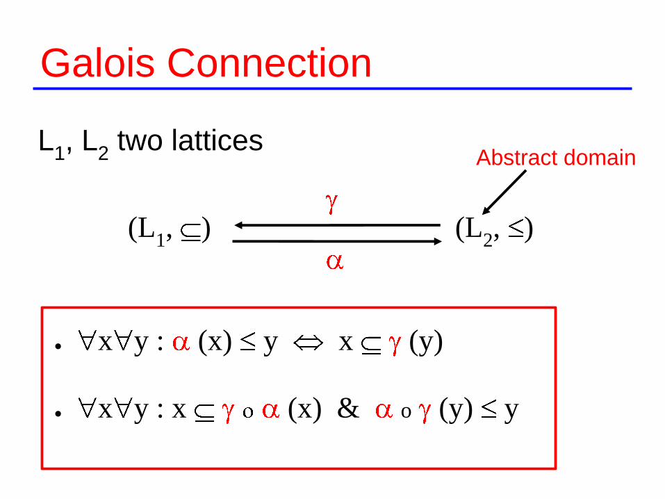
Galois Connection

(L1, ) (L

2, )

L1, L

2two lattices

x y : (x) y x (y)

x y : x (x) & o (y) y

Abstract domain

Fixpoint Approximation

L1

L2

L2

L1

o F o

F

Theorem:lfp F (lfp o F o )

Abstract computation

Concrete computation

Abstracting the Collecting Semantics

• Find a Galois connection:

• Find a function: o F o F#

( ( ), ) ( , )

Abstract Algebra

• Notation: E the set of all environments

• Galois connection:

• , approximated by ,

• Semantics〚op〛approximated by〚op〛#

( (E), ) (E#, )

o〚op〛o 〚op〛#

Abstract Semantic Equations

1: n = 0;

2: while n < 1000 do

3: n = n + 1;

4: end;

5: exit;

E1# = n )

E2

# =〚n = 0〛# E1# E

4#

E3

# = E2# ]- , 999])

E4

# =〚n = n + 1〛# E3#

E5

# = E2# [1000, [)

Methodology

Abstract

Semantics

Collecting

Semantics

Partitioning

Concrete

Semantics

Abstract

Domain

Abstract

Domain

Iterative

Resolution

Algorithms

Tuners

Abstract Domains

• Signs (non relational)

x +, y -, ...

• Intervals (nonrelational):

x [3, 9], y [-23, 4], ...

• Polyhedra (relational):

x + y - 2z 10, ...

• Difference-bound matrices (weakly relational):

y - x z - y

Various kinds of approximations:

Example: intervals

• Iteration 1: E2# = [0, 0]

• Iteration 2: E2

# = [0, 1]

• Iteration 3: E2

# = [0, 2]

• Iteration 4: E2# = [0, 3]

• ...

1: n = 0;

2: while n < 1000 do

3: n = n + 1;

4: end

5: exit

Problem

How to cope with lattices of infinite height?

Solution: automatic extrapolation operators

Methodology

Abstract

Semantics

Collecting

Semantics

Partitioning

Concrete

Semantics

Abstract

Domain

Abstract

Domain

Iterative

Resolution

Algorithms

Tuners

Widening operator

• Abstract union operator:

x y : x x y & y x y

• Enforces convergence: (xn)n 0

Lattice (L, ): L L L

y0

= x0

yn + 1

= yn

xn+1

(yn)n≥0 is ultimately stationary

Widening of intervals

[a, b] [a', b']

If a a' then a else -

If b' b then b else +

Open unstable bounds (jump over the fixpoint)

Widening and Fixpoint

fixpoint

widening

Iteration with widening1: n = 0;

2: while n < 1000 do

3: n = n + 1;

4: end

5: exit

(E2#)

n+1= (E

2#)

n(〚n = 0〛# (E

1#)

n(E

4#)

n)

Iteration 1 (union): E2

# = [0, 0]

Iteration 2 (union): E2

# = [0, 1]

Iteration 3 (widening): E2# = [0, + ] stable

Imprecision at loop exit

1: n = 0;

2: while n < 1000 do

3: n = n + 1;

4: end

5: exit; t[n] = 0; // t has 1500 elements

E5# = [1000, [

False positive!!!

Narrowing operator

Abstract intersection operator:

x y : x y x y

Enforces convergence: (xn)n 0

Lattice (L, ): L L L

y0

= x0

yn + 1

= yn

xn+1

(yn)n≥0 is ultimately stationary

Narrowing of intervals

[a, b] [a', b']

If a = - then a' else a

If b = + then b' else b

Refines open bounds

Narrowing and Fixpoint

fixpoint

widening

narrowing

Iteration with narrowing1: n = 0;

2: while n < 1000 do

3: n = n + 1;

4: end

5: t[n] = 0;

(E2#)

n+1= (E

2#)

n(〚n = 0〛# (E

1#)

n(E

4#)

n)

Beginning of iteration: E2

# = [0, [

Iteration 1: E2

# = [0, 1000] stable

Consequence: E5

# = [1000, 1000]

Methodology

Abstract

Semantics

Collecting

Semantics

Partitioning

Concrete

Semantics

Abstract

Domain

Abstract

Domain

Iterative

Resolution

Algorithms

Tuners

Tuning the abstract domains1: n = 0;

2: k = 0;

3: while n < 1000 do

4: n = n + 1;

5: k = k + 1;

6: end

7: exit

Intervals:

E4# = n k [

Convex polyhedra:

E4# = n k n - k = 0

Annotated Bibliography

References• The historic paper:

– Patrick Cousot & Radhia Cousot. Abstract interpretation: a unified lattice model for static analysis of programs by construction or approximation of fixpoints. In Conference Record of the Fourth Annual ACM SIGPLAN-SIGACT Symposium on Principles of Programming Languages, pages 238—252, Los Angeles, California, 1977. ACM Press, New York, NY, USA.

• Accessible introductions to the theory:

– Patrick Cousot. Semantic foundations of program analysis. In S.S. Muchnick and N.D. Jones, editors, Program Flow Analysis: Theory and Applications, Ch. 10, pages 303—342, Prentice-Hall, Inc., Englewood Cliffs, New Jersey, U.S.A., 1981.

– Patrick Cousot & Radhia Cousot. Abstract interpretation and application to logic programs. Journal of Logic Programming, 13(2—3):103—179, 1992.

• Beyond Galois connections, a presentation of relaxed frameworks:

– Patrick Cousot & Radhia Cousot. Abstract interpretation frameworks. Journal of Logic and Computation, 2(4):511—547, August 1992.

• A thorough description of a static analyzer with all the proofs (difficult to read):

– Patrick Cousot. The Calculational Design of a Generic Abstract Interpreter. Course notes for the NATO International Summer School 1998 on Calculational System Design. Marktoberdorf, Germany, 28 July—9 august 1998, organized by F.L. Bauer, M. Broy, E.W. Dijkstra, D. Gries and C.A.R. Hoare.

References

• The abstract domain of intervals:

– Patrick Cousot & Radhia Cousot. Static Determination of Dynamic Properties of Programs. In B. Robinet, editor, Proceedings of the second international symposium on Programming, Paris, France, pages 106—130, april 13-15 1976, Dunod, Paris.

• The abstract domain of convex polyhedra:

– Patrick Cousot & Nicolas Halbwachs. Automatic discovery of linear restraints among variables of a program. In Conference R ecord of the Fifth Annual ACM SIGPLAN-SIGACT Symposium on Principles of Program ming Languages, pages 84—97, Tucson, Arizona, 1978. ACM Press, New York, NY, USA.

• Weakly relational abstract domains:

– Antoine Miné. The Octagon Abstract Domain. In Analysis, Slicing and Transformation (part of Working Conference on Reverse Engineering), October 2001, IEEE, pages 310-319.

– Antoine Miné. A New Numerical Abstract Domain Based on Difference-Bound Matrices. In Program As Data Objects II, May 2001, LNCS 2053, pages 155-172.

• Classical data flow analysis:

– Steven Muchnick. Advanced Compiler Design and Implementation. Morgan Kaufmann, 1997.