STATIC FRICTION IN RUBBER-METAL CONTACTS WITH … · 2013-07-11 · STATIC FRICTION IN RUBBER-METAL...
184
STATIC FRICTION IN RUBBER-METAL CONTACTS WITH APPLICATION TO RUBBER PAD FORMING PROCESSES Elena Loredana DELADI
Transcript of STATIC FRICTION IN RUBBER-METAL CONTACTS WITH … · 2013-07-11 · STATIC FRICTION IN RUBBER-METAL...
STATIC FRICTION
IN RUBBER-METAL CONTACTS
WITH APPLICATION TO
RUBBER PAD FORMING PROCESSES
Elena Loredana DELADI

This research was carried out under project number MC1.01100 (Static friction in metal forming processes) in the framework of the Strategic Research programme of the Netherlands Institute for Metals Research (www.nimr.nl)
Graduation committee Chairman Prof. dr. F.Eising University of Twente Promotor Prof. dr. ir. D.J. Schipper University of Twente Assistant promotor Dr. ir. M.B. de Rooij University of Twente Members Prof. dr. ir. P. De Baets University of Gent, Belgium Prof. dr. ir. P.M. Lugt Lulea Technical University, Sweden Prof. dr. ir. R. Akkerman University of Twente Prof. dr. ir. A. de Boer University of Twente Prof. dr. ir. J.W.M. Noordermeer University of Twente ISBN-10: 90-77172-22-X ISBN-13: 978-90-77172-22-3 Copyright © 2006 by E.L. Deladi Printed by Print Partners IPSKAMP, The Netherlands

STATIC FRICTION IN RUBBER-METAL CONTACTS WITH APPLICATION TO
RUBBER PAD FORMING PROCESSES
DISSERTATION
to obtain the doctor’s degree at the University of Twente,
on the authority of the rector magnificus, Prof. dr. W.H.M. Zijm,
on account of the decision of the graduation committee, to be publicly defended
on Wednesday 8 November 2006 at 15.00
by
Elena Loredana Deladi born on 2 November 1973 in Cimpulung, Romania

This doctoral dissertation is approved by
promotor Prof. dr. ir. D.J. Schipper assistant promotor Dr. ir. M.B. de Rooij

To my family

Table of contents
1. Introduction 1
1.1 Motivation and objectives of the thesis 1
1.2 Tribology in metal forming processes 1
1.2.1 Rubber pad forming processes 2
1.2.2 Static friction in rubber pad forming processes 3
1.3 Static friction and tribological system 3
1.3.1 Static friction - introduction 3
1.3.2 Static friction and tribological system 4
1.4 Outline of the dissertation 5
2. Static friction 7
2.1 Friction and coefficient of friction 7
2.2 Static friction regime 9
2.3 Friction mechanisms – dynamic friction 11
2.4 Static friction mechanisms 11
2.4.1 Static friction mechanisms in metal-metal contact 12
2.4.2 Static friction mechanisms in rubber friction 14
2.5 Influence of various parameters on the static friction regime 15
2.5.1 Metal-metal contact 15
2.5.1.1 Pressure 16
2.5.1.2 Roughness 17
2.5.1.3 Micro-displacement 17
2.5.1.4 Dwell time 18
2.5.1.5 Temperature 19
2.5.2 Rubber-rigid contact 20
2.5.2.1 Pressure 20
2.5.2.2 Limiting displacement 21
2.5.2.3 Roughness 21
2.6 Summary and conclusions 22

3. Contact of surfaces in a rubber pad forming process
25
3.1 Overview of the tribological system 25
3.2 Mechanical properties of the rubber tool and metal sheet 26
3.2.1 Rubber tool 26
3.2.2 Workpiece 33
3.3 Surface free energy and work of adhesion 34
3.3.1 Equation of state approach 35
3.3.2 Surface tension components approach 35
3.3.3 Contact angle hysteresis approach 36
3.3.4 Surface free energy and work of adhesion sheet 37
3.4 Surface roughness characterization 39
3.4.1 Roughness measurement techniques 40
3.4.2 Measurements 41
3.5 Contact between surfaces 43
3.5.1 Contact area 43
3.5.2 Multi-summit contact (type I contact) 44
3.5.2.1 Summits 45
3.5.3 Overall contact (type II contact) 47
3.5.4 Multi-asperity contact (type III contact) 47
3.6 Contact and friction between rubber pad and metal sheet 49
3.7 Summary and conclusions 50
4. Single-asperity static friction model 51
4.1 Normal loading of elastic bodies 51
4.1.1 Adhesion effect on normal contact of elastic bodies 52
4.1.2 Application: polyurethane-metal contact with adhesion 58
4.2 Normal loading of viscoelastic-rigid asperity couple 59
4.2.1 Modeling the behavior of viscoelastic materials 59
4.2.2 Normal loading of viscoelastic-rigid asperity couple 62
4.2.3 Adhesion effect on the normal contact of a viscoelastic-rigid couple
63
4.2.3.1 Viscoelastic contact with adhesion – theoretical background 63
4.2.3.2 Viscoelastic-rigid contact with adhesion – chosen approach 66

4.3 Tangential loading of elastic bodies 69
4.4 Tangential loading of a viscoelastic-rigid couple 72
4.4.1 Application: viscoelastic-rigid contact 74
4.4.1.1 Viscoelastic-rigid contact with adhesion 77
4.5 Modeling of friction – interfacial layer 78
4.6 Modeling of static friction 81
4.6.1 Mechanism of static friction 81
4.6.2 Modeling of static friction 82
4.6.3 Parametric study 85
4.6.4 Adhesion effect on the single-asperity static friction model 92
4.7 Summary and conclusions 93
5. Multi-asperity static friction model 95
5.1 Viscoelastic/rigid multi-summit contact (type I) 95
5.1.1 Normal loading of viscoelastic/rigid multi-summit contact 95
5.1.2 Tangential loading of viscoelastic/rigid multi-summit contact 97
5.1.3 Static friction of viscoelastic/rigid multi-summit contact 99
5.2 Viscoelastic/rigid multi-asperity contact (type III) 105
5.2.1 Viscoelastic/rigid multi-asperity contact model 105
5.2.2 Viscoelastic/rigid multi-asperity static friction model 109
5.3 Summary and conclusions 118
6. Experimental results and validation of the static friction models
121
6.1 Single-asperity static friction measurements 121
6.1.1 Single-asperity experimental set-up 122
6.1.2 Results 125
6.2 Multi-asperity static friction measurements 130
6.2.1 Experimental set-up 130
6.2.2 Results 133
6.3 Summary and conclusions 137
7. Static friction model – application to rubber pad forming finite element simulations
139
7.1 Static friction model – results 139
7.2 Finite Element model 144
7.3 Summary and conclusions 147
8. Conclusions and recommendations 149
8.1. Conclusions 149
8.2 Recommendations 152
Appendix A 153
Appendix B 155
Appendix C 157
Bibliography 161
Summary 165
List of publications 167
Acknowledgements 169
Biography 171
Nomenclature
Roman symbols a contact radius [m] A area of contact [m2] An nominal contact area [m2] c constant [-] cv radius of the stick area [m] d separation [m] E elasticity modulus [Pa] Fn normal load [N] Ft tangential load [N] g elasticity of the spring [Pa] G shear modulus [Pa] G* complex shear modulus [Pa] G' storage modulus [Pa] G" loss modulus [Pa] hi thickness of the interfacial layer [m] H Heaviside step function [-] k curvature [m-1] Ks kurtosis [-] L length [m] n number of summits per unit area [-] N normal load [N] p pressure [Pa] pn nominal pressure [Pa] r radius [m] R radius [m] Ra center line average surface roughness [m] s summit height [m] s slip [m] sa average summit height [m] Sk skewness [-] t time [s] T temperature [°C] v velocity [m/s] W12 work of adhesion [J/m2] z surface height [m]
Greek symbols α angle of the inclined plane [rad] β average summit radius [m] γ surface free energy [J/m2] γ shear strain [-]

Nomenclature
δl limiting displacement [m] δt tangential displacement [m] ε strain [-] η summit density [m-2] η viscosity of the dashpot [Pa⋅s] μ coefficient of friction [-] μs coefficient of static friction [-] μd coefficient of dynamic friction [-] θ contact angle [º] ν Poisson’s ratio [-] φ(s) summit height density [-] φ(t) creep compliance [Pa-1] ψ(t) stress relaxation function [Pa] σ stress [Pa] σ standard deviation of the surface heights [m] σs standard deviation of the summit heights [m] τ shear stress [Pa] tan δ loss tangent [-]

-1-
Chapter 1
Introduction 1.1 Motivation and objectives of the thesis Numerical simulation of manufacturing processes such as rubber pad forming has been introduced in order to avoid the trial and error procedure used in past for finding and solving the problems encountered in production. Better understanding of friction between tool and workpiece (included in the numerical simulations for instance) may have significant contributions with respect to the prediction of quality of the surface of the products and to the life-time of the tools. A limiting factor in finite element simulations of rubber pad forming processes is an accurate description of the static friction occurring at the workpiece-tool contact interface. The (local) contacts occurring in rubber pad forming processes can be reduced to two basic contact situations, namely:
1) metal-sheet/tool contact and 2) rubber-tool/metal-sheet contact.
The research described in this dissertation focuses on the second contact situation, dealing with an interesting and not very well understood phenomenon – the static friction between rubber pad and metal sheet.
The aims of the thesis are to develop a physically based static friction model for rubber-metal contacts and to validate this model experimentally. The implementation of the static friction model in finite element packages will be a further step towards transferring static friction knowledge to industry. However, this follow-up step is not part of the objective of this thesis. 1.2 Tribology in metal forming processes
The term tribology originates from the Greek word “tribos”, meaning
rubbing. Despite this, the contemporary significance of tribology as science comprises studies of two interacting surfaces in relative motion, and of related subjects. The concern about reducing friction during transport of different materials in order to spare effort has existed from ancient times. However, the conception of tribology as science can be attributed to Leonardo da Vinci (1452-1519), who postulated for the first time a scientific approach of friction. Known also as dealing with friction, lubrication and wear of interacting surfaces, tribology is involved in most of the practical applications. Therefore, a better
Chapter 1
-2-
understanding of the mechanisms occurring in friction of surfaces in contact, either in dry or lubricated conditions, brings significant benefits.
This dissertation deals with static friction in rubber-metal contact, with application to rubber pad forming processes. A description of this process and the relevance of static friction in the process is given in the following sections. 1.2.1 Rubber pad forming processes
Rubber forming process, defined as a deep drawing technique in which one of the tools is replaced by a rubber pad, had its beginning at the end of the 19th century. The technique is mainly used in aircraft industry or for fabrication of prototypes. The advantages of using flexible tools instead of conventional metallic tools are: (i) the flexible pad can be used for several different shapes of workpiece; (ii) the alignment and mismatch problems are eliminated; (iii) lubrication is usually not needed; (iv) the damage of the workpiece surface in contact with the flexible pad is avoided. However, there are some drawbacks, such as: (i) a higher capacity press is usually required; (ii) the tendency to form wrinkles in some processes; (iii) the life time of the flexible pads is limited.
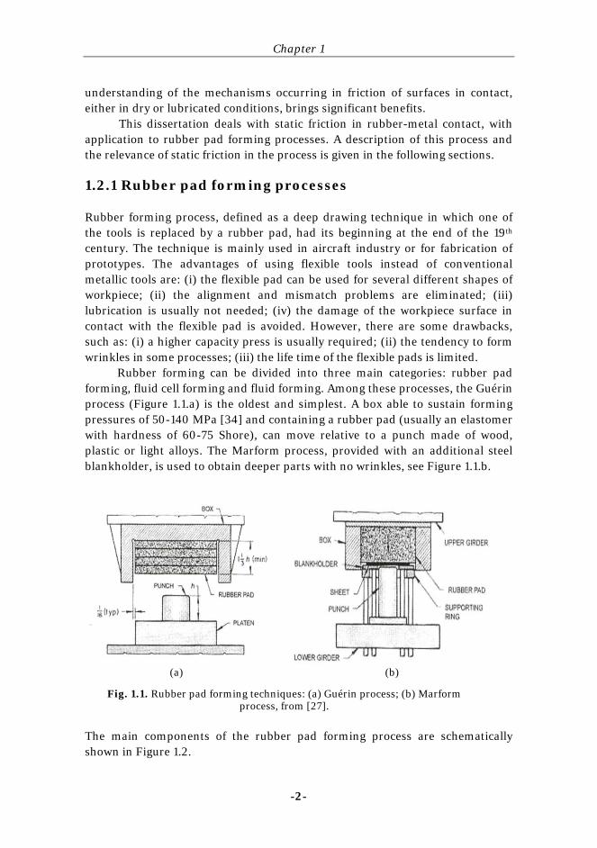
Rubber forming can be divided into three main categories: rubber pad forming, fluid cell forming and fluid forming. Among these processes, the Guérin process (Figure 1.1.a) is the oldest and simplest. A box able to sustain forming pressures of 50-140 MPa [34] and containing a rubber pad (usually an elastomer with hardness of 60-75 Shore), can move relative to a punch made of wood, plastic or light alloys. The Marform process, provided with an additional steel blankholder, is used to obtain deeper parts with no wrinkles, see Figure 1.1.b.
The main components of the rubber pad forming process are schematically shown in Figure 1.2.
Fig. 1.1. Rubber pad forming techniques: (a) Guérin process; (b) Marform process, from [27].
(a) (b)

Introduction
-3-
The container which contains the rubber pad descends applying equal pressure onto the blank. The rubber deforms, filling the empty cavity, thereby inducing conformation of the blank over the die.
In aircraft industry most of the sheet metal parts such as frames, seat parts, ribs, windows, and doors are fabricated using rubber pad forming processes. In other industries, for instance automotive industry, this process is mainly used for prototypes or pilot productions. 1.2.2 Static friction in rubber pad forming processes
In practice static friction is usually associated to the “stick” of surfaces in contact, i.e. the pre-sliding friction, which can be the source of various problems in production. In rubber pad forming processes static friction might affect the accuracy of the product shape, it determines non-uniform plastic strains, it can be a source of noise, and it is also a dissipative process in which energy is lost as heat and/or hysteresis in the case of rubber. Therefore, static friction is normally not desired in metal forming. 1.3 Static friction and tribological system 1.3.1 Static friction - introduction
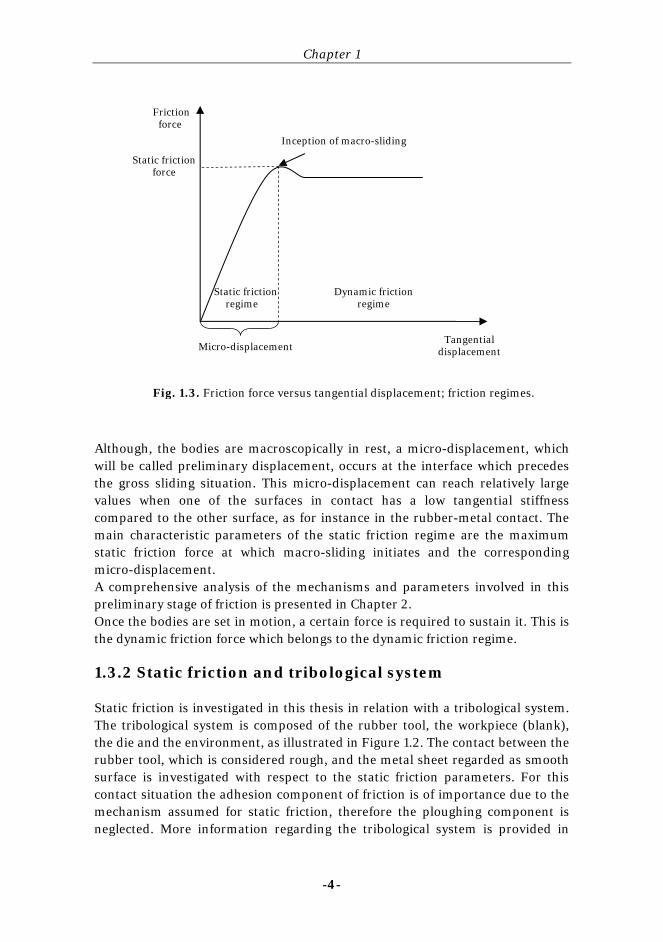
Friction can be separated into two regimes, i.e. the static friction and the dynamic friction regime. In the static friction regime, the friction force increases with increasing tangential displacement up to the value necessary to initiate macro-sliding or gross-sliding of the bodies in contact, as depicted in Figure 1.3.
Rough rubber-tool/ smooth metal sheet
F
F
pad
blank
die
Fig. 1.2. Rubber pad forming – main components; tribological system.
Chapter 1
-4-
Although, the bodies are macroscopically in rest, a micro-displacement, which will be called preliminary displacement, occurs at the interface which precedes the gross sliding situation. This micro-displacement can reach relatively large values when one of the surfaces in contact has a low tangential stiffness compared to the other surface, as for instance in the rubber-metal contact. The main characteristic parameters of the static friction regime are the maximum static friction force at which macro-sliding initiates and the corresponding micro-displacement. A comprehensive analysis of the mechanisms and parameters involved in this preliminary stage of friction is presented in Chapter 2. Once the bodies are set in motion, a certain force is required to sustain it. This is the dynamic friction force which belongs to the dynamic friction regime. 1.3.2 Static friction and tribological system
Static friction is investigated in this thesis in relation with a tribological system. The tribological system is composed of the rubber tool, the workpiece (blank), the die and the environment, as illustrated in Figure 1.2. The contact between the rubber tool, which is considered rough, and the metal sheet regarded as smooth surface is investigated with respect to the static friction parameters. For this contact situation the adhesion component of friction is of importance due to the mechanism assumed for static friction, therefore the ploughing component is neglected. More information regarding the tribological system is provided in
Inception of macro-sliding
Static friction force
Friction force
Tangential displacement Micro-displacement
Dynamic friction regime
Static friction regime
Fig. 1.3. Friction force versus tangential displacement; friction regimes.

Introduction
-5-
Chapter 3. Several parameters such as roughness and cleanliness of the surfaces in
contact, contact pressure, contact (or dwell) time and stiffness of the softer material influence static friction and can be used to reduce it. For instance, rougher and contaminated surfaces result in lower static friction. Thus, the strength of the interface as well as preliminary displacement before macro-sliding will be modelled. Relatively simple material models have been chosen for the rubber pad and interfacial layer. This implies that effects as Schallamach waves or Mullins’s effect are not taken into account. 1.4 Outline of the dissertation
This dissertation deals with a specific application of tribology, the static friction in rubber-metal contact as present in the rubber pad forming process. The motivation and the aims of the research are introduced in this chapter together with the background concerning the related industrial application, i.e. rubber pad forming process.
Chapter 2 deals with definition, mechanisms and parameters characterizing static friction. The parameters required to define the static friction regime are introduced, starting with a short historical background of friction. The mechanisms responsible for static friction as well as for dynamic friction are presented. Then, the influence of several parameters such as pressure, tangential displacement, roughness, contact time, and temperature on this preliminary stage of friction is discussed. A literature survey is presented in this respect for the material couples which are of interest in rubber pad forming, specifically: rubber/metal and metal/metal.
In Chapter 3 the tribological system is reviewed and the relevant properties of the contact between rubber pad and metal sheet are discussed with respect to the material and the surface properties. The viscoelastic properties of the rubber pad and related measurement techniques are presented. Since adhesion is important in friction of rubber-like materials, the surface free energy of materials in contact has been investigated. Surface roughness plays a significant role in contact, thus in friction between the rubber pad and the metal sheet. Therefore, surface roughness parameters are introduced together with measurement techniques. Depending on the relation between the real contact area and the apparent contact area, various approaches can be used to model the contact between the rubber pad and the metal sheet. These approaches are briefly discussed.
The single-asperity static friction model is discussed in Chapter 4. First, the normal contact between a viscoelastic sphere and a rigid flat is modeled using a modified Hertz theory, in which the viscoelastic behavior is incorporated through a mechanical model. Then, when a tangential load is subsequently
Chapter 1
-6-
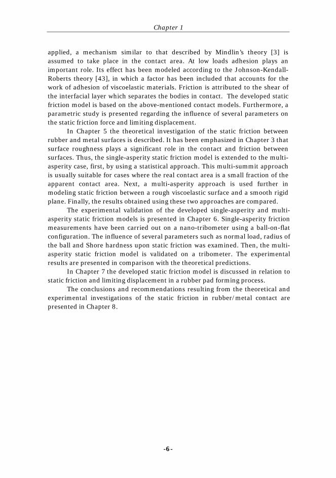
applied, a mechanism similar to that described by Mindlin’s theory [3] is assumed to take place in the contact area. At low loads adhesion plays an important role. Its effect has been modeled according to the Johnson-Kendall-Roberts theory [43], in which a factor has been included that accounts for the work of adhesion of viscoelastic materials. Friction is attributed to the shear of the interfacial layer which separates the bodies in contact. The developed static friction model is based on the above-mentioned contact models. Furthermore, a parametric study is presented regarding the influence of several parameters on the static friction force and limiting displacement. In Chapter 5 the theoretical investigation of the static friction between rubber and metal surfaces is described. It has been emphasized in Chapter 3 that surface roughness plays a significant role in the contact and friction between surfaces. Thus, the single-asperity static friction model is extended to the multi-asperity case, first, by using a statistical approach. This multi-summit approach is usually suitable for cases where the real contact area is a small fraction of the apparent contact area. Next, a multi-asperity approach is used further in modeling static friction between a rough viscoelastic surface and a smooth rigid plane. Finally, the results obtained using these two approaches are compared. The experimental validation of the developed single-asperity and multi-asperity static friction models is presented in Chapter 6. Single-asperity friction measurements have been carried out on a nano-tribometer using a ball-on-flat configuration. The influence of several parameters such as normal load, radius of the ball and Shore hardness upon static friction was examined. Then, the multi-asperity static friction model is validated on a tribometer. The experimental results are presented in comparison with the theoretical predictions. In Chapter 7 the developed static friction model is discussed in relation to static friction and limiting displacement in a rubber pad forming process. The conclusions and recommendations resulting from the theoretical and experimental investigations of the static friction in rubber/metal contact are presented in Chapter 8.
-7-
Chapter 2
Static friction
Introduction
This chapter deals with definition, mechanisms and parameters regarding static friction. Starting with a short historical background of friction, the parameters required to define the static friction regime are introduced. The mechanisms responsible for dynamic friction as well as for static friction are presented. Then, the influence of several parameters such as pressure, tangential displacement, roughness, dwell time, and temperature on this preliminary stage of friction will be discussed. A literature survey is presented in this respect for the two couple of materials of interest, rubber/metal and metal/metal.
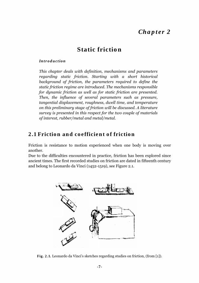
2.1 Friction and coefficient of friction Friction is resistance to motion experienced when one body is moving over another. Due to the difficulties encountered in practice, friction has been explored since ancient times. The first recorded studies on friction are dated in fifteenth century and belong to Leonardo da Vinci (1452-1519), see Figure 2.1.
Fig. 2.1. Leonardo da Vinci’s sketches regarding studies on friction, (from [1]).

Chapter 2
-8-
His observations became two hundred of years later two of the well-known laws of sliding (dynamic) friction introduced by Guillaume Amontons (1663-1705), namely: 1. Friction force is directly proportional to the applied load. 2. Friction force is independent of the apparent area of contact. Leonardo da Vinci introduced also the concept of coefficient of friction (μ) as the ratio of the friction force Ff to normal load N:
μ = Ff/N (2.1) Johann Andreas von Segner (1704-1777) was the first who made distinction between static and dynamic (or kinetic) friction. The easiest set-up to understand static friction consists in a body placed on an inclined plane (Figure 2.2) as proposed by Leonhard Euler (1707-1783).
The force which maintains the body in rest (no macroscopic relative motion) on the tilted plane is the static friction force. The force needed to initiate gross sliding is the maximum static friction force Fs. The dynamic friction force Fd is the force required to sustain motion. The coefficient of friction can be also defined as the tangent of the angle of the inclined plane. The body will remain in rest for an angle θ less than a certain value α and it will start sliding down if the inclination angle exceeds α. Writing the load balance equations for the body from Figure 2.2, the coefficient of static friction is given by:
μs =Fs/N =W⋅sinα/W⋅cosα = tan α (2.2) The coefficient of static friction is typically larger than the dynamic one, but it can be also equal to the coefficient of dynamic friction. More detailed experimental studies on friction were conducted by Charles-
Fig. 2.2. Forces acting on a body in sliding motion.
→ W
N →
Ff
→
θ

Static friction
-9-
Augustin Coulomb (1736-1806) who completed the laws of friction with the third law: 3. Dynamic friction force is independent of the sliding velocity. These empirical laws have been proved to be valid under certain conditions for many material couples. However, these laws are not valid for all material couples. For instance, the coefficient of friction between polymers sliding against themselves or against metals or ceramics decreases by increasing the normal load (i.e. contact pressure), which is in contradiction with the first law. The third law is also not obeyed in contact between polymers and other materials. A typical curve indicating the dependence of coefficient of dynamic friction on velocity is shown in Figure 2.3. At higher velocities the rubber becomes stiffer, then the contact area decreases determining a reduction of the coefficient of dynamic friction.
Although the above-mentioned laws are generally called laws of friction in fact they were obtained empirically using dynamic friction data. 2.2 Static friction regime
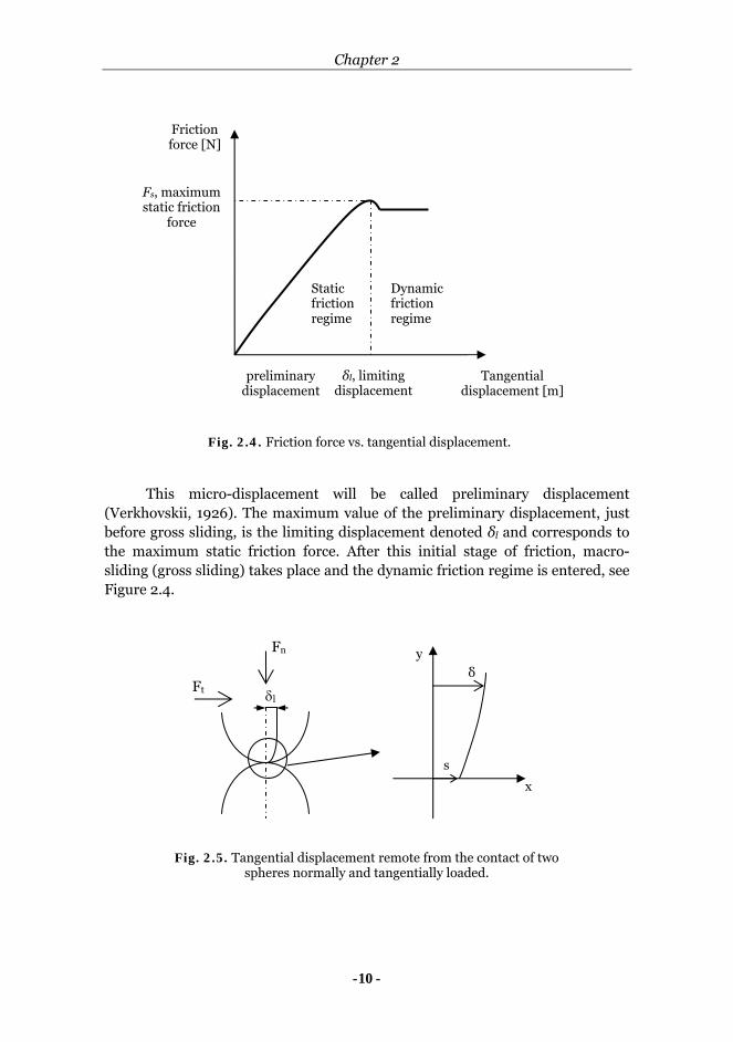
Figure 2.4 typically describes the relation between the friction force and the tangential displacement between two contacting bodies. Before macro-sliding or gross-sliding is initiated, micro-slip occurs at the interface. A distinction must be made between slip s, denoting relative displacement of adjacent points on a portion of the contact surface, and micro-displacement δ, a term used for relative tangential displacement of points remote from the contact, as shown schematically in Figure 2.5.
v [m/s]
μd [-]
Fig. 2.3. Dependence of coefficient of dynamic friction on velocity (rubber friction).
Chapter 2
-10-
This micro-displacement will be called preliminary displacement
(Verkhovskii, 1926). The maximum value of the preliminary displacement, just before gross sliding, is the limiting displacement denoted δl and corresponds to the maximum static friction force. After this initial stage of friction, macro-sliding (gross sliding) takes place and the dynamic friction regime is entered, see Figure 2.4.
δl
Fn
Ft
Fig. 2.5. Tangential displacement remote from the contact of two spheres normally and tangentially loaded.
δ
s
x
y
Fig. 2.4. Friction force vs. tangential displacement.
preliminary displacement
Tangential displacement [m]
Friction force [N]
δl, limiting displacement
Fs, maximum static friction
force
Static friction regime
Dynamic friction regime

Static friction
-11-
2.3 Friction mechanisms – dynamic friction At a microscopic scale, friction is mainly caused by adhesion and deformation and can be written as:
Ff = Fadhesion + Fdeformation (2.3) Depending on the materials in contact, these two factors can be caused by different mechanisms.
According to Tabor and Bowden [28], dry friction between metals can be attributed to adhesion and deformation (or ploughing). The adhesion component of friction occurs while trying to shear local “welded” areas between contacting asperities. Adhesion is not the only resistance encountered during motion of one body over another. If one of the surfaces in contact is harder and rougher than the other one, the hard one will plough through the soft surface giving rise to the deformation term of friction. The magnitude of the force is strongly dependent on the geometry of the ploughing body and the hardness of the softest body. The energy is dissipated in this way by plastic deformation.
Rubber friction has also a component due to adhesion and one due to deformation. The adhesion term is regarded as a surface effect and occurs during making and breaking of bonds on a molecular level. The deformation component, also called hysteresis friction, is caused by the delayed recovery (viscoelastic behavior) of the deformed rubber. The energy is dissipated through the internal damping in the rubber bulk, therefore is considered a bulk property. Nevertheless, it is experienced as a resisting force to the movement of one body relative to the other body at the interface. An insight into the molecular dissipation mechanisms shows that there are three main ways, namely: through chemical mechanisms, phononic dissipation and electronic dissipation [27]. The chemical mechanism involves energy associated with the breaking of chemical bonds. The phononic dissipation is related to the atomic vibrations within the bulk material and is associated with frictional heating. The electronic dissipation involves the excitation of electrons at the sliding interface.
2.4 Static friction mechanisms A few mechanisms have been found in literature indicated to be responsible for static friction. These mechanisms might involve elastic deformation or plastic deformation of the softer material in contact or local welding or creep of asperities. They will be presented in the following for the contact between metals as well as for the contact between rubber and metal (regarded as rigid).
Chapter 2
-12-
2.4.1 Static friction mechanisms in metal-metal contact
Most studies on static friction relate the static friction force to the tangential displacement before sliding on macro-scale occurs. Rankin [2] found experimentally that a preliminary displacement does exist before the point of sliding is reached. In his experiments carried out on flat surfaces of steel in contact with cast iron this displacement was elastic. In the experiments of Verhovskii [2], performed on flat contact surfaces of various metals, the preliminary displacement was non-elastic.
The static friction mechanisms found in literature for metallic materials in contact are described below. They are essential for the understanding of static friction.
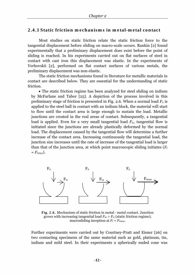
• The static friction regime has been analyzed for steel sliding on indium by McFarlane and Tabor [25]. A depiction of the process involved in this preliminary stage of friction is presented in Fig. 2.6. When a normal load Fn is applied to the steel ball in contact with an indium block, the material will start to flow until the contact area is large enough to sustain the load. Metallic junctions are created in the real areas of contact. Subsequently, a tangential load is applied. Even for a very small tangential load Ft1, tangential flow is initiated since the junctions are already plastically deformed by the normal load. The displacement caused by the tangential flow will determine a further increase of the contact area. Increasing continuously the tangential load, the junction size increases until the rate of increase of the tangential load is larger than that of the junction area, at which point macroscopic sliding initiates (Ft = Ftmax).
Further experiments were carried out by Courtney-Pratt and Eisner [26] on two contacting specimens of the same material such as gold, platinum, tin, indium and mild steel. In their experiments a spherically ended cone was
Ft2
Fn Fn
Ft1 Ftmax
Fn
Fig. 2.6. Mechanism of static friction in metal - metal contact. Junction grows with increasing tangential load Ft2 > Ft1 (static friction regime);
macrosliding inception at Ft = Ftmax.

Static friction
-13-
loaded against a plane and the displacement of the metallic bodies was measured. The results confirm the theory presented by McFarlane and Tabor. They also emphasized that the plastic deformation process determines the build-up of the friction force while the surface interaction is responsible for the final magnitude of the static friction force. Accordingly, the film of contaminants reduces the maximum friction due to the reduction in contact area.
• Chang and co-workers [4] assumed in their theoretical static friction coefficient model for metallic rough surfaces that only the asperities which have not reached their elastic limit can contribute to the static friction force. The maximum static friction force is the sum of all tangential forces causing plastic flow of the individual pre-stressed asperities. So, the plastic deformation of asperities is the mechanism responsible for static friction
• Johnson [2] investigated the micro-displacement between a hard steel ball and the flat end of a hard steel roller under the action of steady and oscillating tangential forces less than the static friction force. The quantitative results of the experiments are in good agreement with theoretical elastic theory proposed by Mindlin [3]. This theory has been developed for two elastic bodies which are loaded normally and tangentially against each other. According to Mindlin, if there is no slip between the contacting surfaces, the distribution of the shear stress goes asymptotically to infinite at the boundary of the contact circle. However, in practice this infinite shear stress has to be relieved in some manner, for instance by relative slipping of surfaces over an annulus which spreads radially inwards with increasing tangential load (Figure 2.7).
A A
Fn
Ft
A-A
stick area
slip area
Ft1 Ft2 Ftmax
inception of macro-sliding
Fig. 2.7. Evolution of the contact area (top view) according to Mindlin theory.

Chapter 2
-14-
It is worth mentioning that the assumption of elastic bodies can be made for very hard, smooth bodies or for very elastic ones.
• Two temperature-related mechanisms for static friction were proposed by Galligan and McCullough [6]. At low temperature the mechanism involves creep of asperities leading to motion, while for higher temperature the mechanism implies local sintering or welding of asperities and the motion occurs when these asperities break apart of each other.
• The nature of static friction was investigated by Persson et al. [5] using molecular dynamics simulations. They focused on boundary lubrication at high pressures (1 GPa), which is typical for the contact between hard materials. The pinning of lubricant molecules on the solids is described by springs with bending elasticity. Stiff springs imply a very small static friction of the system, whereas soft springs determine a larger static friction force due to the elastic instabilities.
2.4.2 Static friction mechanisms in rubber friction
The literature survey revealed that static friction in rubber friction was less studied compared with the dynamic regime. Most of the papers describe experimental studies but none of them gives a complete explanation of the mechanism responsible for static friction. A review of these papers is presented in the following.
Experiments were carried out by Barquins [10] on glass hemispherical samples in contact with soft elastomer samples. The evolution of the contact area was recorded by means of a camera mounted on an optical microscope. The superposition of the frames showed a contact area which comprises a central adhesive zone, surrounded by an annulus of slip. The mechanism seems to be similar to Mindlin’s theoretical approach, illustrated in Figure 2.7.
The experiments of Adachi et al. [14] carried out on rubber balls in contact with glass plates revealed also the process of partial slip and its propagation with increasing tangential load as described theoretically by Mindlin.
The static friction force was investigated by Roberts and Thomas [9] for
v
Fig. 2.8. Sliding friction mechanism, from [5].
Static friction
-15-
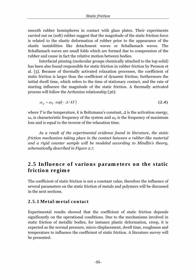
smooth rubber hemispheres in contact with glass plates. Their experiments carried out on (soft) rubber suggest that the magnitude of the static friction force is related to the elastic deformation of rubber prior to the appearance of the elastic instabilities like detachment waves or Schallamach waves. The Schallamach waves are small folds which are formed due to compression of the rubber and cause in fact the relative motion between bodies.
Interfacial pinning (molecular groups chemically attached to the top solid) has been also found responsible for static friction in rubber friction by Persson et al. [5]. Because of thermally activated relaxation processes, the coefficient of static friction is larger than the coefficient of dynamic friction; furthermore the initial dwell time, which refers to the time of stationary contact, and the rate of starting influence the magnitude of the static friction. A thermally activated process will follow the Arrhenius relationship [36]:
( )kT/expp Δωω −⋅= 0 (2.4)
where T is the temperature, k is Boltzmann’s constant, Δ is the activation energy, ω0 is characteristic frequency of the system and ωp is the frequency of maximum loss and is equal to the inverse of the relaxation time.
As a result of the experimental evidence found in literature, the static friction mechanism taking place in the contact between a rubber-like material and a rigid counter sample will be modeled according to Mindlin’s theory, schematically described in Figure 2.7.
2.5 Influence of various parameters on the static friction regime The coefficient of static friction is not a constant value, therefore the influence of several parameters on the static friction of metals and polymers will be discussed in the next sections. 2.5.1 Metal-metal contact Experimental results showed that the coefficient of static friction depends significantly on the operational conditions. Due to the mechanisms involved in static friction of metallic bodies, for instance plastic deformation, creep, it is expected as the normal pressure, micro-displacement, dwell time, roughness and temperature to influence the coefficient of static friction. A literature survey will be presented.

Chapter 2
-16-
2.5.1.1 Pressure Nolle & Richardson [7] pointed out that the two classical laws of friction (Amontons-Coulomb) can not entirely describe the friction properties of real metal surfaces since they do not take into account the surface contamination, material plastic deformation and time dependency. By considering these factors, the relation between the coefficient of static friction and the apparent contact pressure can be plotted as in Figure 2.9. The apparent contact pressure is defined as the ratio of the normal load to nominal contact area. At low pressures, region I, the coefficient of static friction is constant. Both surfaces are covered by contaminant films and friction is mainly due to shearing of these films. Contaminant films are less reactive than clean metals therefore the friction forces are small in this region. Increasing the contact pressure, the surface film is progressively broken. Some metal-metal contact occurs and friction force rises sharply (region II). In region III substantial metal-metal contact takes place. The coefficient of static friction is again independent of pressure, but is much larger than in region I. The large contact pressures from region IV determine extensive plastic deformation of surfaces. The coefficient of friction significantly decreases with increasing pressure and eventually becomes zero when the material fails in compression. The zero-coefficient of static friction at large pressures is debatable if the mechanism responsible for static friction in metal-metal contact is taken into account, see section 2.4.1.
Experimental results found in literature for the coefficients of static friction between dry steel surfaces indicate some qualitative agreement with theoretical trends showed in Figure 2.9.
I II III IV
Apparent contact pressure [Pa]
Coe
ffic
ien
t of
st
atic
fri
ctio
n [
-]
Fig. 2.9. Qualitative description of the dependence of the coefficient of static friction on pressure, from [5].

Static friction
-17-
Chang et al. [4] found, based on a theoretical model, that at high pressures the coefficient of static friction between two rough metallic surfaces (steel on steel) decreases with increasing contact pressure. At high pressures most asperities are plastically deformed. Only a few asperities which have not reached their elastic limit can sustain a tangential force. As a result the friction force is small compared with the contact load, resulting in a very small coefficient of friction. Similar results were reported elsewhere by Broniec and Lankiewicz [8] between flat steel surfaces. 2.5.1.2 Roughness In Chang’s static friction model for metallic rough surfaces [4] the effect of surface roughness was studied by varying the plasticity index. The plasticity index depends on material properties and surface topography. Smooth surfaces and hard materials have a low plasticity index and the contact is mostly elastic, while rough surfaces and soft materials have a high plasticity index and the contact is typically plastic. The results indicated that the coefficient of static friction decreases as the plasticity index increases. A high plasticity index means sharp asperities which are mostly plastically deformed, resulting in a small tangential force which can be sustained before macro-sliding. For very rough surfaces the effect of normal load on the coefficient of static friction diminishes, similar results were also reported elsewhere [8, 9]. 2.5.1.3 Micro-displacement
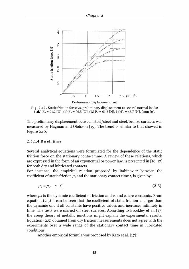
The experimental investigation performed by Johnson [2] on a steel ball
in contact with the flat end of a hard steel roller showed that the static friction force rises linearly with preliminary displacement (Figure 2.10). Close to the point of sliding this dependence becomes non-linear. It can be observed that increasing the normal load results in an increase of preliminary displacement and static friction force. The results plotted in Figure 2.9 were obtained using a ball of 9.52⋅10-3 [m] diameter for a pressure range of 6.55⋅105 to 1.28⋅106 [Pa].
Chapter 2
-18-
The preliminary displacement between steel/steel and steel/bronze surfaces was measured by Hagman and Olofsson [15]. The trend is similar to that showed in Figure 2.10. 2.5.1.4 Dwell time Several analytical equations were formulated for the dependence of the static friction force on the stationary contact time. A review of these relations, which are expressed in the form of an exponential or power law, is presented in [16, 17] for both dry and lubricated contacts. For instance, the empirical relation proposed by Rabinovicz between the coefficient of static friction μs and the stationary contact time ts is given by:
21
csds tc ⋅+= μμ (2.5)
where μd is the dynamic coefficient of friction and c1 and c2 are constants. From equation (2.5) it can be seen that the coefficient of static friction is larger than the dynamic one if all constants have positive values and increases infinitely in time. The tests were carried on steel surfaces. According to Brockley et al. [17] the creep theory of metallic junctions might explain the experimental results. Equation (2.5) obtained from dry friction measurements does not agree with the experiments over a wide range of the stationary contact time in lubricated conditions. Another empirical formula was proposed by Kato et al. [17]:
Fig. 2.10. Static friction force vs. preliminary displacement at several normal loads: ( ) Fn = 91.2 [N], (x) Fn = 76.5 [N], (Δ) Fn = 61.8 [N], (+)Fn = 46.7 [N], from [2].
Preliminary displacement [m]
Stat
ic f
rict
ion
forc
e [N
]
0.5 1 1.5 2 2.5 (× 10-6)
8.9
17
.8
2
6.7
35.
6
4
4.5

Static friction
-19-
( ) ( )4
300csds tcexp ⋅−⋅−−= μμμμ (2.6)
where μ0 is the asymptotic value of μs when ts → ∞, μd is the value of μs when ts → 0, nearly equal to the dynamic coefficient of friction and c3 , c4 are constants which depend on the properties of the lubricant applied and the surface topography. Equation (2.6) predicts a finite value of the coefficient of static friction even for a very long contact time (ts → ∞). Surfaces were made of cast iron. This equation shows a good agreement with the experimental results for a wide range of the dwell time. Both equations are shown schematically in Figure 2.11.
As an example, the values of the constants in the equations (2.5) and (2.6) obtained on cast iron surfaces lubricated with naphthene mineral oil are given in Table 2.1. Table 2.1. The values of the parameters of equations (2.5) and (2.6), from [17].
lubricant: naphtane
mineral oil μd μ0 c1 c2 c3 c4
Rabinowicz eq. (2.5) 0.156 - 0.079 0.284 - -
Kato eq. (2.6) 0.156 0.450 - - 0.286 0.671 2.5.1.5 Temperature The temperature effect on the coefficient of static friction was experimentally investigated by Galligan and McCullough [6] on copper and brass. They found
μs [-]
ts [s]
Rabinowicz Kato
Fig. 2.11. The variation of coefficient of static friction with stationary contact time.

Chapter 2
-20-
that, at relatively low temperatures, the coefficient of static friction decreases with increasing temperature and, after passing a minimum, it starts to increase with temperature, see Figure 2.12.
At low temperature the mechanism involves creep of asperities. In copper on copper contact, this low temperature regime was between 20°C and 60°C. Increasing the temperature in region (I), the amount of creep increases, thus a smaller tangential force is required to initiate macro-sliding. Conclusively, the coefficient of static friction decreases with increasing temperature in the low-temperature regime. After passing through a minimum which depends on the materials in contact, the coefficient of static friction increases for higher temperatures (70 to 120°C in copper on copper contact). In region (II) static friction is related to the mechanism of welding of asperities and breaking of these junctions. When the temperature increases, the junctions become stronger and a higher tangential force is required to cause macro-sliding.
2.5.2 Rubber-rigid contact Static friction of polymers was not widely studied, however the data found in literature shows that it is affected by various parameters such as pressure, micro-displacement and roughness. These dependencies will be presented and discussed further. 2.5.2.1 Pressure Experiments carried out on glass lenses in contact with a rubber flat surface by
(I) creep of asperities
(II) welding of asperities
μs [-]
T(°C)
Fig. 2.12. Qualitative description of the dependence of the coefficient of static friction on temperature, adapted from [6].
Static friction
-21-
Barquins and Roberts [11] showed that the coefficient of static friction decreases if the normal load increases.
A relationship between the maximum static friction force Fs and normal load N was obtained by Tarr and Rhee [12] from their experiments on a filled phenolic resin/cast iron material couple in a flat on flat configuration. Accordingly, Fs = μs⋅Nβ where the exponent β varies from 1.03 to 1.41 for organic materials (phenolic resin reinforced with asbestos and filled with minerals) and from 1.1 to 1.37 for semi-metallic materials (phenolic resin reinforced with steel fiber and filled with iron, graphite and minerals). 2.5.2.2 Limiting displacement The micro-displacement prior gross sliding is an important parameter of the static friction regime as it was already mentioned. The dependence of this micro-displacement on the coefficient of static friction (or maximum static friction force) is presented in the following.
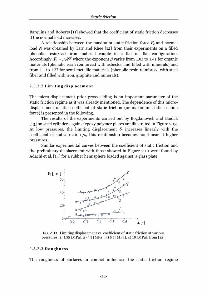
The results of the experiments carried out by Bogdanovich and Baidak [13] on steel cylinders against epoxy polymer plates are illustrated in Figure 2.13. At low pressures, the limiting displacement δl increases linearly with the coefficient of static friction μs, this relationship becomes non-linear at higher pressures.
Similar experimental curves between the coefficient of static friction and the preliminary displacement with those showed in Figure 2.10 were found by Adachi et al. [14] for a rubber hemisphere loaded against a glass plate.
2.5.2.3 Roughness The roughness of surfaces in contact influences the static friction regime
Fig.2.13. Limiting displacement vs. coefficient of static friction at various pressures: 1) 1.55 [MPa], 2) 4.5 [MPa], 3) 6.5 [MPa], 4) 10 [MPa], from [13].
δl [μm]
μs[-]
Chapter 2
-22-
regarding the limiting displacement and the coefficient of static friction. Bogdanovich and Baidak [13] investigated the effect of surface roughness
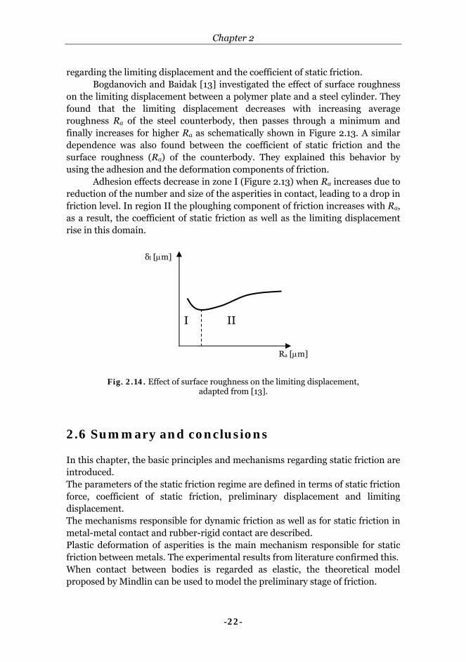
on the limiting displacement between a polymer plate and a steel cylinder. They found that the limiting displacement decreases with increasing average roughness Ra of the steel counterbody, then passes through a minimum and finally increases for higher Ra as schematically shown in Figure 2.13. A similar dependence was also found between the coefficient of static friction and the surface roughness (Ra) of the counterbody. They explained this behavior by using the adhesion and the deformation components of friction. Adhesion effects decrease in zone I (Figure 2.13) when Ra increases due to reduction of the number and size of the asperities in contact, leading to a drop in friction level. In region II the ploughing component of friction increases with Ra, as a result, the coefficient of static friction as well as the limiting displacement rise in this domain.
2.6 Summary and conclusions In this chapter, the basic principles and mechanisms regarding static friction are introduced. The parameters of the static friction regime are defined in terms of static friction force, coefficient of static friction, preliminary displacement and limiting displacement. The mechanisms responsible for dynamic friction as well as for static friction in metal-metal contact and rubber-rigid contact are described. Plastic deformation of asperities is the main mechanism responsible for static friction between metals. The experimental results from literature confirmed this. When contact between bodies is regarded as elastic, the theoretical model proposed by Mindlin can be used to model the preliminary stage of friction.
δl [μm]
Ra [μm]
I II
Fig. 2.14. Effect of surface roughness on the limiting displacement, adapted from [13].

Static friction
-23-
Two temperature-related static friction mechanisms have been found in contact between metallic surfaces. They consist in creep of asperities at low temperatures and in welding of asperities at higher temperatures. Less attention has been paid to the mechanisms of static friction between rubber and other materials. As a result of the experimental evidence found in literature, Mindlin’s approach of a contact area comprising a stick and slip zone which evolves until gross sliding occurs has been chosen to describe the mechanism of static friction in rubber-metal contacts. Experimental results from literature showed that the static friction regime in metal friction as well as in rubber friction depends on several parameters such as pressure, dwell time, temperature and roughness. A literature survey has been presented in this respect.
A theoretical model for predicting static friction of rubber-metal systems is not available in literature. The relationships found are based on experimental results.

Chapter 2
-24-
-25-
Chapter 3
Contact of surfaces in a rubber pad forming process
Introduction
In this chapter, the tribological system is reviewed and the relevant properties of the contact between rubber pad and metal sheet are discussed with respect to the material and surface properties. The viscoelastic properties of the rubber pad are described as well as the measurement techniques. Since adhesion can play an essential role in friction of rubber-like materials, the surface free energy of materials in contact has been investigated. Surface roughness plays a significant role in contact and friction between the rubber pad and the metal sheet. Therefore, surface roughness parameters are introduced together with measurement techniques. Depending on the relation between the real contact area and the apparent contact area, different approaches can be used to model the contact between the rubber pad and the metal sheet. These approaches are briefly discussed.
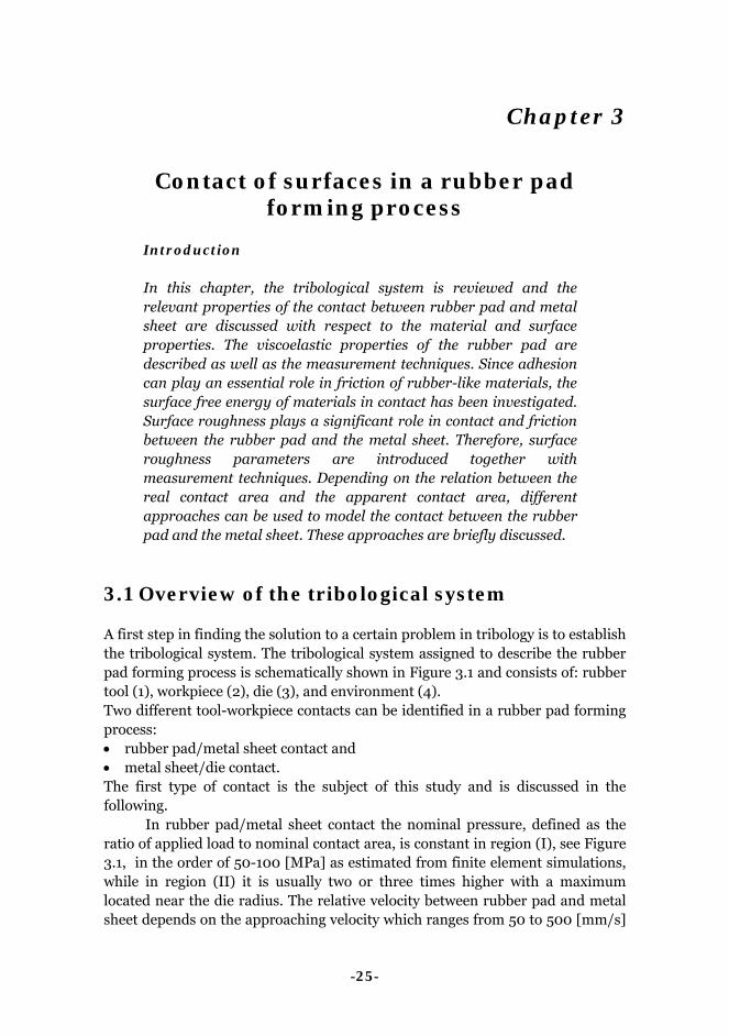
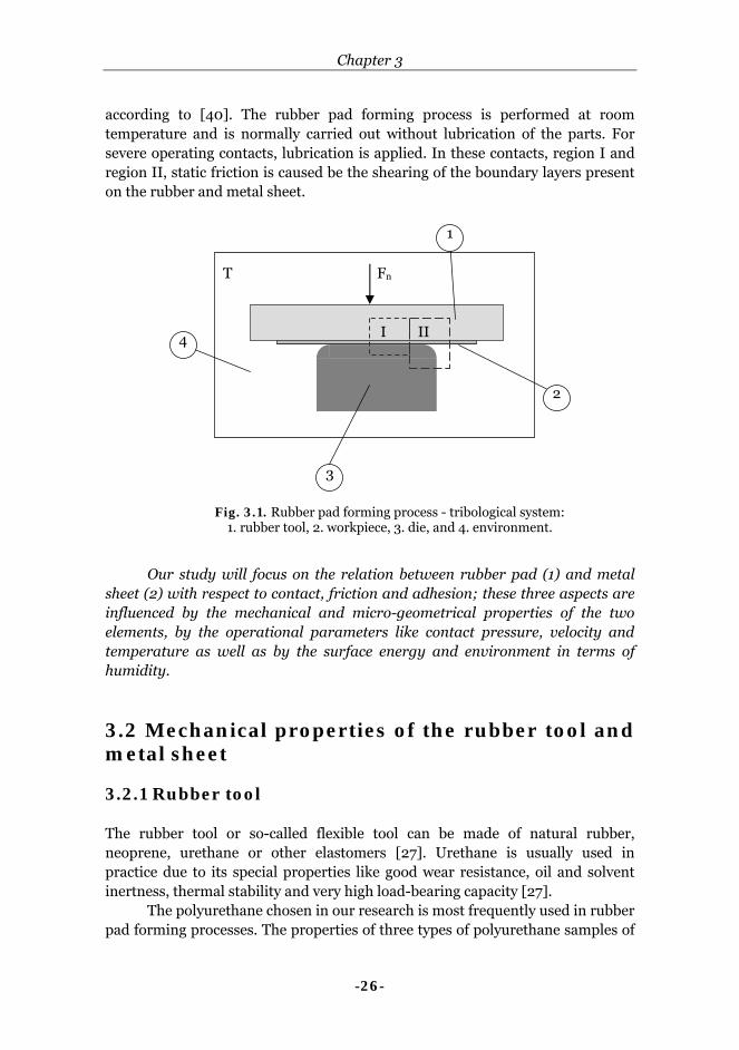
3.1 Overview of the tribological system A first step in finding the solution to a certain problem in tribology is to establish the tribological system. The tribological system assigned to describe the rubber pad forming process is schematically shown in Figure 3.1 and consists of: rubber tool (1), workpiece (2), die (3), and environment (4). Two different tool-workpiece contacts can be identified in a rubber pad forming process: • rubber pad/metal sheet contact and • metal sheet/die contact. The first type of contact is the subject of this study and is discussed in the following. In rubber pad/metal sheet contact the nominal pressure, defined as the ratio of applied load to nominal contact area, is constant in region (I), see Figure 3.1, in the order of 50-100 [MPa] as estimated from finite element simulations, while in region (II) it is usually two or three times higher with a maximum located near the die radius. The relative velocity between rubber pad and metal sheet depends on the approaching velocity which ranges from 50 to 500 [mm/s]
Chapter 3
-26-
according to [40]. The rubber pad forming process is performed at room temperature and is normally carried out without lubrication of the parts. For severe operating contacts, lubrication is applied. In these contacts, region I and region II, static friction is caused be the shearing of the boundary layers present on the rubber and metal sheet.
Our study will focus on the relation between rubber pad (1) and metal sheet (2) with respect to contact, friction and adhesion; these three aspects are influenced by the mechanical and micro-geometrical properties of the two elements, by the operational parameters like contact pressure, velocity and temperature as well as by the surface energy and environment in terms of humidity. 3.2 Mechanical properties of the rubber tool and metal sheet 3.2.1 Rubber tool The rubber tool or so-called flexible tool can be made of natural rubber, neoprene, urethane or other elastomers [27]. Urethane is usually used in practice due to its special properties like good wear resistance, oil and solvent inertness, thermal stability and very high load-bearing capacity [27]. The polyurethane chosen in our research is most frequently used in rubber pad forming processes. The properties of three types of polyurethane samples of
Fig. 3.1. Rubber pad forming process - tribological system: 1. rubber tool, 2. workpiece, 3. die, and 4. environment.
4
3
1
2
T Fn
I II

Contact of surfaces in rubber pad forming processes
-27-
different hardness (80, 90 and 95 Shore A) are listed in Appendix A, Table A.1 It is important to mention that the polyurethane is a viscoelastic material, which means that it shows the characteristics of both an elastic solid and a viscoelastic fluid. As a result, some other tests have been carried out in order to determine the specific viscoelastic properties. These tests can be divided into two main categories:
• dynamic tests (or frequency/temperature domain measurements) and • transient tests (time domain measurements).
Dynamic tests From this category, the Dynamic Mechanical Analysis (DMA) was the technique used to measure the dynamic properties of the polyurethane samples. The tests were carried out on a Myrenne ATM3 torsion pendulum at a frequency of 1 Hz and 0.1 % strain. The samples were first cooled to -100°C and then subsequently heated at a rate of 1°C/min up to 220 ºC. The basic properties obtained from a DMA experiment include the storage modulus (G'), the loss modulus (G") and the loss tangent (tan δ) as a function of temperature (T), as shown schematically in Figure 3.2.
The storage modulus G' is defined as the stress in phase with strain divided by the strain in a sinusoidal shear deformation mode [28] and it is a measure of the energy stored and recovered per cycle. The loss modulus G" is defined as the stress 90° out of phase with the strain divided by the strain [28] and is a measure of the energy dissipated or lost as heat per cycle of cyclic deformation. The loss
Fig. 3.2. Storage modulus, loss modulus and loss tangent as a function of temperature (adapted from [34]).
tan δ
G'
stor
age
mod
ulu
s G
' [N
/m2 ]
lo
ss m
odu
lus
G"
[N/m
2 ]
loss
tan
gen
t ta
n δ
[-]
temperature [°C]
G"
Chapter 3
-28-
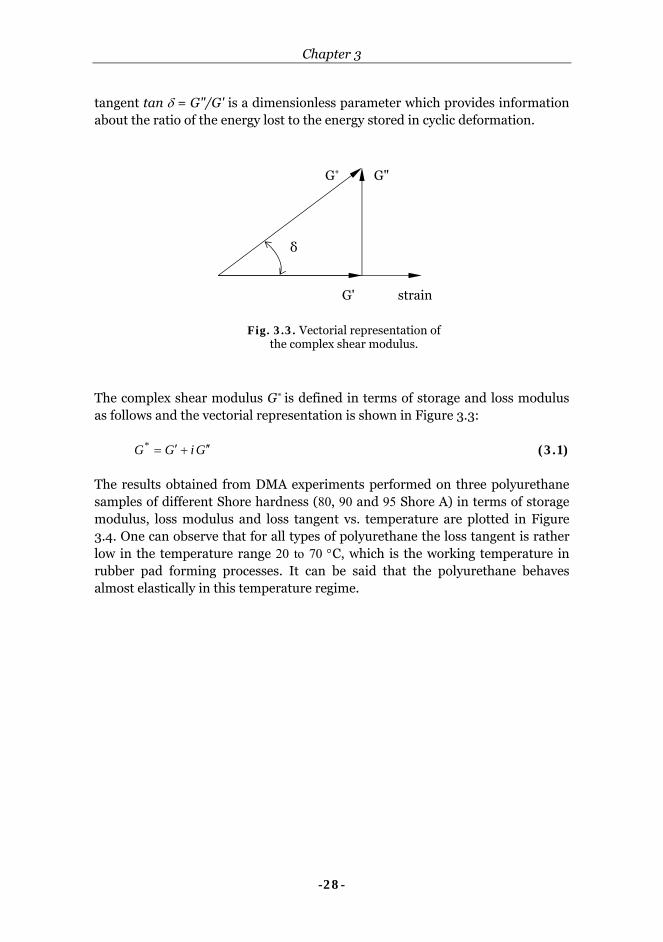
tangent tan δ = G"/G' is a dimensionless parameter which provides information about the ratio of the energy lost to the energy stored in cyclic deformation.
The complex shear modulus G* is defined in terms of storage and loss modulus as follows and the vectorial representation is shown in Figure 3.3:
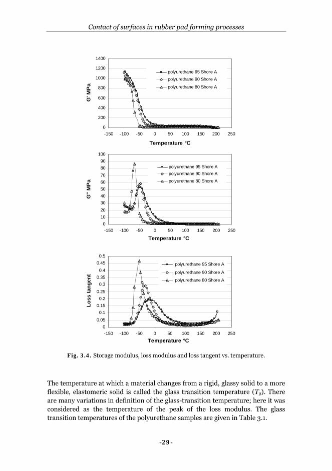
GiGG* ′′+′= (3.1) The results obtained from DMA experiments performed on three polyurethane samples of different Shore hardness (80, 90 and 95 Shore A) in terms of storage modulus, loss modulus and loss tangent vs. temperature are plotted in Figure 3.4. One can observe that for all types of polyurethane the loss tangent is rather low in the temperature range 20 to 70 °C, which is the working temperature in rubber pad forming processes. It can be said that the polyurethane behaves almost elastically in this temperature regime.
strain
G*
δ
Fig. 3.3. Vectorial representation of the complex shear modulus.
G"
G'
Contact of surfaces in rubber pad forming processes
-29-
The temperature at which a material changes from a rigid, glassy solid to a more flexible, elastomeric solid is called the glass transition temperature (Tg). There are many variations in definition of the glass-transition temperature; here it was considered as the temperature of the peak of the loss modulus. The glass transition temperatures of the polyurethane samples are given in Table 3.1.
Fig. 3.4. Storage modulus, loss modulus and loss tangent vs. temperature.
0
200
400
600
800
1000
1200
1400
-150 -100 -50 0 50 100 150 200 250
Temperature °C
G' M
Pa
polyurethane 95 Shore Apolyurethane 90 Shore A
polyurethane 80 Shore A
0102030405060708090
100
-150 -100 -50 0 50 100 150 200 250
Temperature °C
G"
MP
a
polyurethane 95 Shore Apolyurethane 90 Shore Apolyurethane 80 Shore A
00.050.1
0.150.2
0.250.3
0.350.4
0.450.5
-150 -100 -50 0 50 100 150 200 250
Temperature °C
Loss
tang
ent
polyurethane 95 Shore A
polyurethane 90 Shore A
polyurethane 80 Shore A

Chapter 3
-30-
Table 3.1 Glass transition temperatures and reference temperatures of the polyurethane samples.
Material Tg [°C] Tr [°C]
polyurethane 80 Shore A -65.4 -15.4 polyurethane 90 Shore A -45.3 4.7 polyurethane 95 Shore A -45.5 4.5
The measured data can be converted into frequency data at a certain
temperature using the Williams-Landel-Ferry (WLF) equation [40]. Accordingly, the values of any viscoelastic property obtained at temperature T and frequency ω (ω = 2πf, rad/s) can be related to a reference temperature (Tr = Tg + 50°C) by a frequency shift aTω. The values of the glass transition temperature and reference temperature for each material are given in Table 3.1. The WLF equation is given by:
r
rT TT.
)TT(.alog−+−−
=5101
86810 (3.2)
The storage modulus as a function of the frequency can be expressed as: ( ) ( )roTo T,a'GT,'G ωω = (3.3) In order to reduce the experimental data to a certain temperature, for instance room temperature T0 = 20 °C, the shift factor for the new temperature has to be calculated:
r
rT TT.
)TT(.alog−+−−
=0
010 5101
8680
(3.4)
Then, the shift in decades Q is given by:
01010 TT alogalogQ −= (3.5)
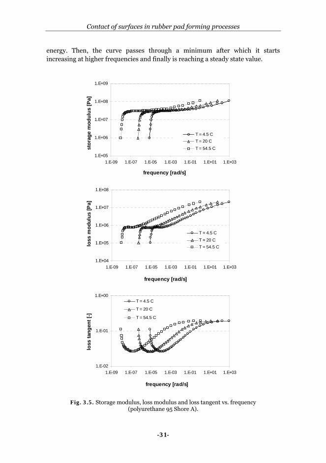
Thus, each data point recorded at (ω, T) with log10 ω as abscissa has to be shifted by an amount Q to correspond to the new temperature T0. The storage modulus, loss modulus and loss tangent as a function of frequency are given in Figure 3.5 for the polyurethane 95 shore hardness A. These data are presented for three temperatures (reference temperature (Tr), room temperature (T0), and Tf = Tg + 100 ° C) within the temperature range where the WLF law is applicable, Tg < T < Tg + 100 ° C. It can be observed that the loss tangent decreases in the low frequency regime, this means that the energy stored in the material is larger than the dissipated
Contact of surfaces in rubber pad forming processes
-31-
energy. Then, the curve passes through a minimum after which it starts increasing at higher frequencies and finally is reaching a steady state value.
Fig. 3.5. Storage modulus, loss modulus and loss tangent vs. frequency (polyurethane 95 Shore A).
1.E+05
1.E+06
1.E+07
1.E+08
1.E+09
1.E-09 1.E-07 1.E-05 1.E-03 1.E-01 1.E+01 1.E+03
frequency [rad/s]
stor
age
mod
ulus
[Pa]
T = 4.5 CT = 20 CT = 54.5 C
1.E+04
1.E+05
1.E+06
1.E+07
1.E+08
1.E-09 1.E-07 1.E-05 1.E-03 1.E-01 1.E+01 1.E+03
frequency [rad/s]
loss
mod
ulus
[Pa]
T = 4.5 CT = 20 CT = 54.5 C
1.E-02
1.E-01
1.E+00
1.E-09 1.E-07 1.E-05 1.E-03 1.E-01 1.E+01 1.E+03
frequency [rad/s]
loss
tang
ent [
-]
T = 4.5 C
T = 20 C
T = 54.5 C
Chapter 3
-32-
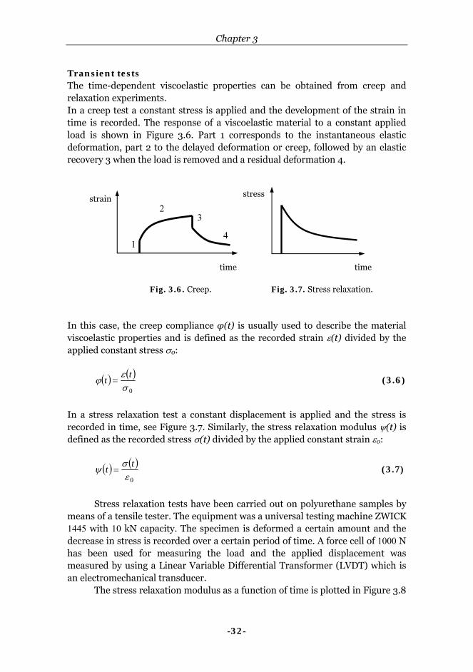
Transient tests The time-dependent viscoelastic properties can be obtained from creep and relaxation experiments. In a creep test a constant stress is applied and the development of the strain in time is recorded. The response of a viscoelastic material to a constant applied load is shown in Figure 3.6. Part 1 corresponds to the instantaneous elastic deformation, part 2 to the delayed deformation or creep, followed by an elastic recovery 3 when the load is removed and a residual deformation 4.
In this case, the creep compliance φ(t) is usually used to describe the material viscoelastic properties and is defined as the recorded strain ε(t) divided by the applied constant stress σ0:
( ) ( )0σ
εϕ tt = (3.6)
In a stress relaxation test a constant displacement is applied and the stress is recorded in time, see Figure 3.7. Similarly, the stress relaxation modulus ψ(t) is defined as the recorded stress σ(t) divided by the applied constant strain ε0:
( ) ( )0ε
σψ tt = (3.7)
Stress relaxation tests have been carried out on polyurethane samples by means of a tensile tester. The equipment was a universal testing machine ZWICK 1445 with 10 kN capacity. The specimen is deformed a certain amount and the decrease in stress is recorded over a certain period of time. A force cell of 1000 N has been used for measuring the load and the applied displacement was measured by using a Linear Variable Differential Transformer (LVDT) which is an electromechanical transducer. The stress relaxation modulus as a function of time is plotted in Figure 3.8
1
2 3
4
strain
time time
stress
Fig. 3.6. Creep. Fig. 3.7. Stress relaxation.
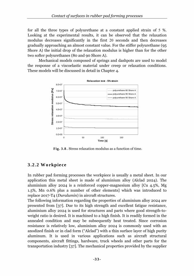
Contact of surfaces in rubber pad forming processes
-33-
for all the three types of polyurethane at a constant applied strain of 5 %. Looking at the experimental results, it can be observed that the relaxation modulus decreases significantly in the first 20 seconds and then decreases gradually approaching an almost constant value. For the stiffer polyurethane (95 Shore A) the initial drop of the relaxation modulus is higher than for the other two softer polyurethanes (80 and 90 Shore A).
Mechanical models composed of springs and dashpots are used to model the response of a viscoelastic material under creep or relaxation conditions. These models will be discussed in detail in Chapter 4.
3.2.2 Workpiece In rubber pad forming processes the workpiece is usually a metal sheet. In our application this metal sheet is made of aluminium alloy (Alclad 2024). The aluminium alloy 2024 is a reinforced copper-magnesium alloy [Cu 4.5%, Mg 1.5%, Mn 0.6% plus a number of other elements] which was introduced to replace 2017-T4 (Duralumin) in aircraft structures. The following information regarding the properties of aluminium alloy 2024 are presented from [37]. Due to its high strength and excellent fatigue resistance, aluminium alloy 2024 is used for structures and parts where good strength-to-weight ratio is desired. It is machined to a high finish. It is readily formed in the annealed condition and may be subsequently heat treated. Since corrosion resistance is relatively low, aluminium alloy 2024 is commonly used with an anodized finish or in clad form (“Alclad”) with a thin surface layer of high purity aluminum. It is used in various applications such as aircraft structural components, aircraft fittings, hardware, truck wheels and other parts for the transportation industry [37]. The mechanical properties provided by the supplier
Relaxation test - 5% strain
0.E+00
1.E+07
2.E+07
3.E+07
4.E+07
5.E+07
6.E+07
7.E+07
8.E+07
0 50 100 150Time [s]
Stre
ss r
elax
atio
n m
odul
us [P
a] polyurethane 80 Shore A
polyurethane 95 Shore A
polyurethane 90 Shore A
Fig. 3.8. Stress relaxation modulus as a function of time.
Chapter 3
-34-
(Stork-Fokker) are summarized in Appendix A, Table A.2. The provided aluminum sheet is 0.7 [mm] thick.
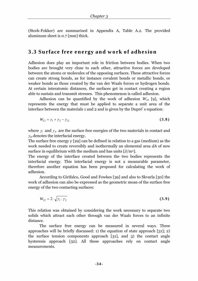
3.3 Surface free energy and work of adhesion Adhesion does play an important role in friction between bodies. When two bodies are brought very close to each other, attractive forces are developed between the atoms or molecules of the opposing surfaces. These attractive forces can create strong bonds, as for instance covalent bonds or metallic bonds, or weaker bonds as those created by the van der Waals forces or hydrogen bonds. At certain interatomic distances, the surfaces get in contact creating a region able to sustain and transmit stresses. This phenomenon is called adhesion.
Adhesion can be quantified by the work of adhesion W12 [9], which represents the energy that must be applied to separate a unit area of the interface between the materials 1 and 2 and is given by the Dupré’ s equation:
122112 γγγ −+=W (3.8)
where γ1 and γ 2 are the surface free energies of the two materials in contact and γ12 denotes the interfacial energy. The surface free energy γ [29] can be defined in relation to a gas (medium) as the work needed to create reversibly and isothermally an elemental area dA of new surface in equilibrium with the medium and has units [J/m2]. The energy of the interface created between the two bodies represents the interfacial energy. This interfacial energy is not a measurable parameter, therefore another equation has been proposed for calculating the work of adhesion. According to Girifalco, Good and Fowkes [39] and also to Skvarla [30] the work of adhesion can also be expressed as the geometric mean of the surface free energy of the two contacting surfaces:
2112 2 γγ ⋅⋅=W (3.9)
This relation was obtained by considering the work necessary to separate two solids which attract each other through van der Waals forces to an infinite distance. The surface free energy can be measured in several ways. Three approaches will be briefly discussed: 1) the equation of state approach [31]; 2) the surface tension components approach [31], and 3) the contact angle hysteresis approach [32]. All these approaches rely on contact angle measurements.
Contact of surfaces in rubber pad forming processes
-35-
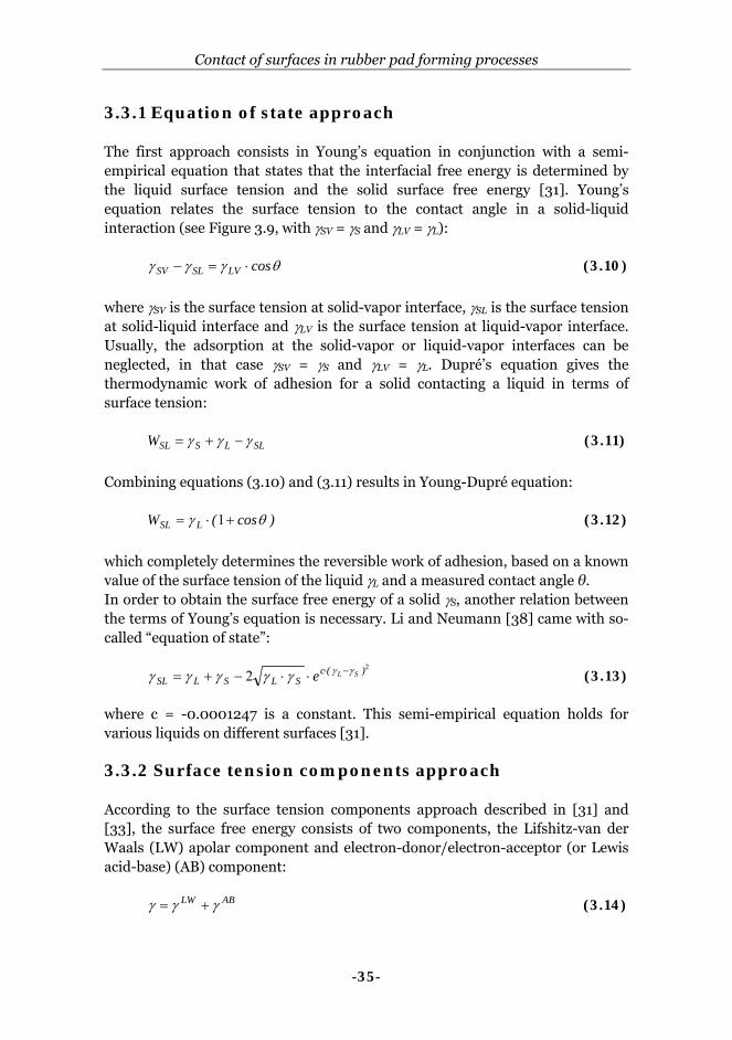
3.3.1 Equation of state approach The first approach consists in Young’s equation in conjunction with a semi-empirical equation that states that the interfacial free energy is determined by the liquid surface tension and the solid surface free energy [31]. Young’s equation relates the surface tension to the contact angle in a solid-liquid interaction (see Figure 3.9, with γSV = γS and γLV = γL): θγγγ cosLVSLSV ⋅=− (3.10)
where γSV is the surface tension at solid-vapor interface, γSL is the surface tension at solid-liquid interface and γLV is the surface tension at liquid-vapor interface. Usually, the adsorption at the solid-vapor or liquid-vapor interfaces can be neglected, in that case γSV = γS and γLV = γL. Dupré’s equation gives the thermodynamic work of adhesion for a solid contacting a liquid in terms of surface tension: SLLSSLW γγγ −+= (3.11)
Combining equations (3.10) and (3.11) results in Young-Dupré equation: )cos(W LSL θγ +⋅= 1 (3.12)
which completely determines the reversible work of adhesion, based on a known value of the surface tension of the liquid γL and a measured contact angle θ. In order to obtain the surface free energy of a solid γS, another relation between the terms of Young’s equation is necessary. Li and Neumann [38] came with so-called “equation of state”:
22 )(c
SLSLSLSLe γγγγγγγ −⋅⋅⋅−+= (3.13)
where c = -0.0001247 is a constant. This semi-empirical equation holds for various liquids on different surfaces [31]. 3.3.2 Surface tension components approach According to the surface tension components approach described in [31] and [33], the surface free energy consists of two components, the Lifshitz-van der Waals (LW) apolar component and electron-donor/electron-acceptor (or Lewis acid-base) (AB) component: ABLW γγγ += (3.14)

Chapter 3
-36-
The Lifshitz-van der Waals component of the work of adhesion can be calculated using the geometric mean approach as follows:
LWS
LWL
LWSLW γγ ⋅⋅= 2 (3.15)
and the Lewis acid-base term is determined by the following combining rule:
⎥⎦⎤
⎢⎣⎡ ⋅+⋅⋅= −++−
LSLSAB
SLW γγγγ2 (3.16)
where −
Sγ is the electron-donor (Lewis base) and +Sγ is the electron-acceptor
(Lewis acid) parameter. The total work of adhesion can be expressed as [33]:
⎥⎦⎤
⎢⎣⎡ ⋅+⋅+⋅⋅2=+1⋅= −++−
LSLSLWL
LWSLW γγγγγγθγ )cos( (3.17)
By performing contact angle measurements for three liquids and having known their surface tension and components ( −
Lγ , +Lγ , LW
Lγ ), the system formed by equation (3.17) written for each liquid can be solved with respect to the solid surface free energy components ( −
Sγ , +Sγ , LW
Sγ ). It is worth mentioning that the choice of liquid triads is very important; as it was shown by Radelczuk et al. [33], not any liquid triad can be used to calculate the solid surface free energy components. Table 3.2 presents a summary of the liquids used for contact angle measurement and “good triplets” [33].
Table 3.2 Liquids that can be used for contact angle measurements [33].
Water (W) Liquid triads
Glycerol (G)
Formamide (F) Bipolar liquids
Ethylene glycol (EG)
Diiodomethane (D) Apolar liquids
1-Bromonaphthalene (B)
D-W-F
D-W-G
D-W-EG
B-W-F
B-W-G
B-W-EG
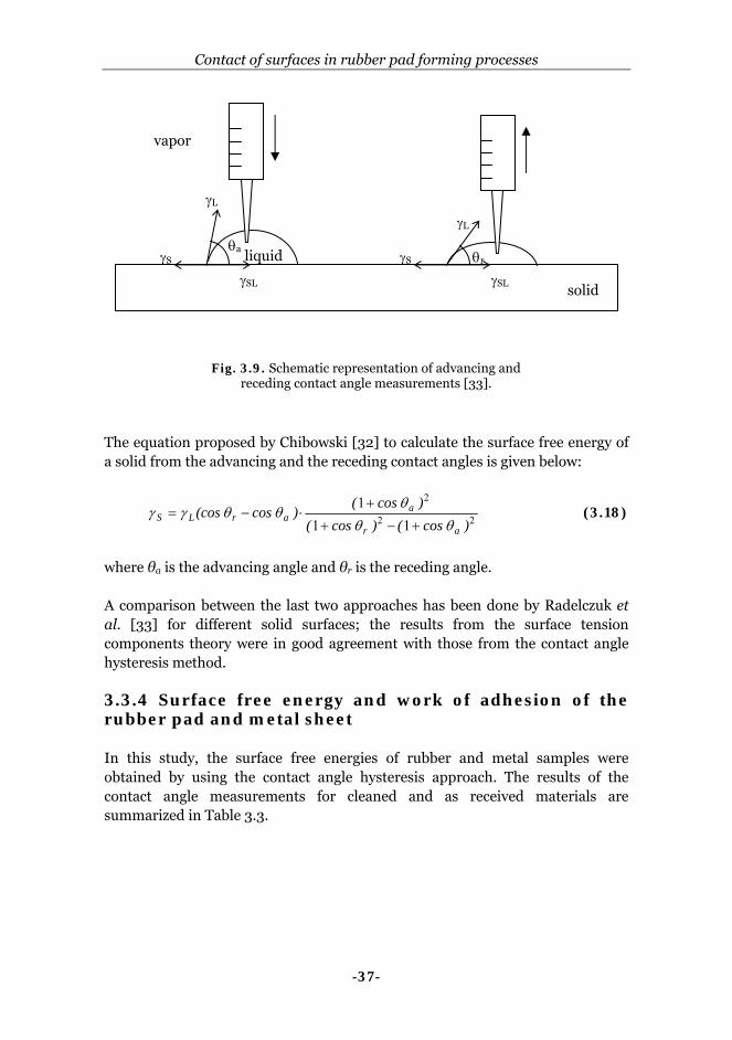
3.3.3 Contact angle hysteresis approach The third approach is based on three measurable parameters: advancing and receding angles and the liquid surface tension. The advancing and receding angles can be measured using the syringe method [33]. A schematic representation of this method is shown in Figure 3.9.
Contact of surfaces in rubber pad forming processes
-37-
The equation proposed by Chibowski [32] to calculate the surface free energy of a solid from the advancing and the receding contact angles is given below:
22
2
111
)cos()cos()cos(
)cos(cosar
aarLS θθ
θθθγγ
+−+
+⋅−= (3.18)
where θa is the advancing angle and θr is the receding angle. A comparison between the last two approaches has been done by Radelczuk et al. [33] for different solid surfaces; the results from the surface tension components theory were in good agreement with those from the contact angle hysteresis method. 3.3.4 Surface free energy and work of adhesion of the rubber pad and metal sheet In this study, the surface free energies of rubber and metal samples were obtained by using the contact angle hysteresis approach. The results of the contact angle measurements for cleaned and as received materials are summarized in Table 3.3.
θa θr
γL
γS
γSL
γS
γL
γSL solid
liquid
vapor
Fig. 3.9. Schematic representation of advancing and receding contact angle measurements [33].

Chapter 3
-38-
Table 3.3 Advancing and receding contact angle and surface free energy.
Material
(clean surfaces)
Advancing
contact
angle, θa
Receding
contact
angle, θr
γS
(mJ/m2)
Fibroflex 80 Shore A (clean surface) 92 56 27 Fibroflex 90 Shore A (clean surface) 106 52 16 Fibroflex 95 Shore A (clean surface) 87 34 28 Al alloy (2024) (clean surface) 63 38 47 Steel (clean surface) 52 32 55 Al alloy (2024) (as received) 79 29 34 Steel(as received) 75 34 37
The liquid used was water and the surfaces were cleaned with ethanol and
dried with air. Looking at the advancing contact angles in Table 3.3 it is observed that the rubber samples have hydrophobic surfaces (θ > 90º) while the metal surfaces are hydrophilic (θ < 90º). Two advancing contact angle measurements are presented in Figure 3.10. The surface free energy of solids was calculated with equation (3.18). As expected, the rubber samples have a relatively low surface energy compared with metals. The surface free energy is smaller for contaminated surfaces (as received) as indicated by the results obtained for aluminum and steel surfaces. In industrial applications (rubber pad forming process) the surfaces are not cleaned.
Having determined the surface free energies of the two materials in
contact (rubber pad-aluminum sheet, aluminum sheet-steel die) the work of
θa
Fig. 3.10. Advancing contact angle measurements: steel surface – left hand side; polyurethane 80 Shore A – right hand side.
θa

Contact of surfaces in rubber pad forming processes
-39-
adhesion for rubber-metal and metal-metal contacts was calculated with equation (3.9).The results are listed in Table 3.4. The results show that the resulting work of adhesion is smaller when one of the materials in contact has a low surface energy (polyurethane).
Table 3.4 Work of adhesion.
Material combination Work of adhesion
(mJ/m2)
Fibroflex 80 Shore A – aluminum alloy 71 Fibroflex 90 Shore A – aluminum alloy 55 Fibroflex 95 Shore A– aluminum alloy 73 Fibroflex 95 Shore A– steel 78 Steel – aluminum alloy 102
3.4 Surface roughness characterization A rough surface is composed of peaks (or asperities) and valleys of different amplitudes and spacings as schematically shown in Figure 3.11. A comprehensive analysis of surface roughness is given in [18], [19].
Two parameters commonly used to describe random rough surfaces
regarding their amplitude are the average roughness (Ra) and standard deviation (σ) of the surface heights or the root mean square (RMS). In order to define these parameters, a mean line is established so that the area delimited by the
mean line
L
peaks or asperities
valleys
z
dz
p(z)
x
Fig. 3.11. Surface roughness description (adapted from [18]).
Chapter 3
-40-
roughness profile and the mean line, above and below the mean line, is the same, as schematically shown in Figure 3.11. The average roughness is given by equation:
∫⋅=L
a dxzL
R0
1 (3.19)
where z(x) is the height of the surface above the mean line and L is the sampling length. The root-mean-square RMS or standard deviation σ of the height of the surface from the mean line is defined by:
∫⋅=L
dxzL
0
22 1σ (3.20)
The probability height distribution p(z) denotes the probability that the height of a certain point on the surface to be situated between z and (z + dz). This probability distribution is often similar to the normal or Gaussian probability function (see Figure 3.11) and is expressed as: ( ) ( )22211 22 σπσ ⋅−⋅⋅⋅= −− /zexp)z(p / (3.21) with σ the RMS roughness value.
All above-presented parameters are related to the variations in height of the surface. One parameter which describes the surface roughness from lateral or spatial point of view is the density of the peaks ηp, which is the number of peaks per unit length. 3.4.1 Roughness measurement techniques Several measurement techniques are used to obtain surface height data. They can be classified according to the physical principle involved into following: mechanical stylus, optical methods, scanning probe microscopy (SPM), fluid methods, electrical methods, and electron microscopy methods [19]. The first two techniques are typically used in engineering and manufacturing applications and are of interest for this study, while the other are used for nano-scale to atomic scale roughnesses.
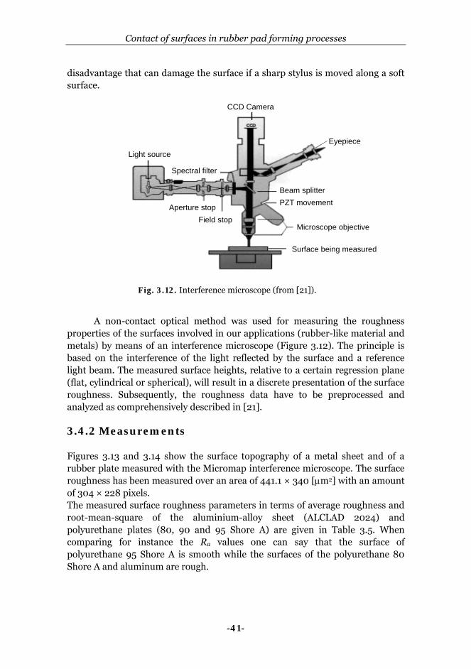
In the mechanical stylus method a stylus is moved with a constant velocity across the surface. The vertical motion due to the surface height deviations is amplified and recorded. This is a contact-type instrument which has the
Contact of surfaces in rubber pad forming processes
-41-
disadvantage that can damage the surface if a sharp stylus is moved along a soft surface.
A non-contact optical method was used for measuring the roughness
properties of the surfaces involved in our applications (rubber-like material and metals) by means of an interference microscope (Figure 3.12). The principle is based on the interference of the light reflected by the surface and a reference light beam. The measured surface heights, relative to a certain regression plane (flat, cylindrical or spherical), will result in a discrete presentation of the surface roughness. Subsequently, the roughness data have to be preprocessed and analyzed as comprehensively described in [21]. 3.4.2 Measurements Figures 3.13 and 3.14 show the surface topography of a metal sheet and of a rubber plate measured with the Micromap interference microscope. The surface roughness has been measured over an area of 441.1 × 340 [μm2] with an amount of 304 × 228 pixels. The measured surface roughness parameters in terms of average roughness and root-mean-square of the aluminium-alloy sheet (ALCLAD 2024) and polyurethane plates (80, 90 and 95 Shore A) are given in Table 3.5. When comparing for instance the Ra values one can say that the surface of polyurethane 95 Shore A is smooth while the surfaces of the polyurethane 80 Shore A and aluminum are rough.
Fig. 3.12. Interference microscope (from [21]).
Light source
Spectral filter
Eyepiece
Beam splitter
Microscope objective
PZT movement
Surface being measured
CCD Camera
Aperture stopField stop
Light source
Spectral filter
Eyepiece
Beam splitter
Microscope objective
PZT movement
Surface being measured
CCD Camera
Aperture stopField stop

Chapter 3
-42-
Table 3.5 Surface roughness parameters.
Material Ra (μm) RMS (μm)
Aluminum alloy 0.371 0.481 Polyurethane 95 Shore A 0.013 0.017 Polyurethane 90 Shore A 0.072 0.112 Polyurethane 80 Shore A 0.978 1.441
Fig. 3.13. Surface height data – aluminum sheet.
Fig. 3.14. Surface height data – polyurethane sample (polyurethane 95 Shore A).
Contact of surfaces in rubber pad forming processes
-43-
Different from the surface of the polyurethane samples, the aluminum sheet has a certain pattern, this means an anisotropic surface.
In summary, the properties of the rubber pad and metal sheet have been discussed as well as the methods used to determine them. DMA and relaxation tests have been carried out on the rubber samples in order to evaluate the viscoelastic properties. The surface free energies of the metal and polyurethane samples have been obtained based on contact angle measurements. The roughness parameters of surfaces in contact have been also obtained. 3.5 Contact between surfaces An essential step in studying friction between bodies consists in modeling the contact between them. Different approaches can be used depending on the properties of the materials in contact. They will be discussed in the following sections. 3.5.1 Contact area When two bodies touch each other a contact area is created. This geometrical area is called apparent or nominal contact area. In reality, the contact will occur between their summits on many small areas. The sum of all these areas gives the real contact area. In Figure 3.15 the upper surface has been considered rough and the lower one is taken as smooth. Depending on the relation between the nominal contact area and the real contact area we can divide the contact between surfaces into three main categories: I. multi-summit contact in which the real contact area is a very small fraction of the apparent contact area. II. overall contact in which the asperities are squeezed giving rise to a giant “asperity”. In this case the real contact area is almost equal to the apparent contact area. III. multi-asperity contact is an intermediate contact situation. Here, the contact is not determined by the local maxima and also not by the global shape of the surface. All these contact situations are further discussed and the approaches used in modeling are presented.

Chapter 3
-44-
3.5.2 Multi-summit contact (type I contact) The Greenwood-Williamson [20] approach is suitable for type I contact where the real contact area is a small fraction of the nominal contact area.
Surface 2
β
Surface 1
s
z
d
Mean plane surface heights
Mean plane summit heights
σs
sa
Fig. 3.16. Modeling surface roughness and contact of rough surfaces (statistical approach).
Fn
Fn
a.
c.
R
Fn
b.
Fig. 3.15. Types of contact: a. multi-summit contact; b. single-like asperity contact; c. multi-asperity contact.
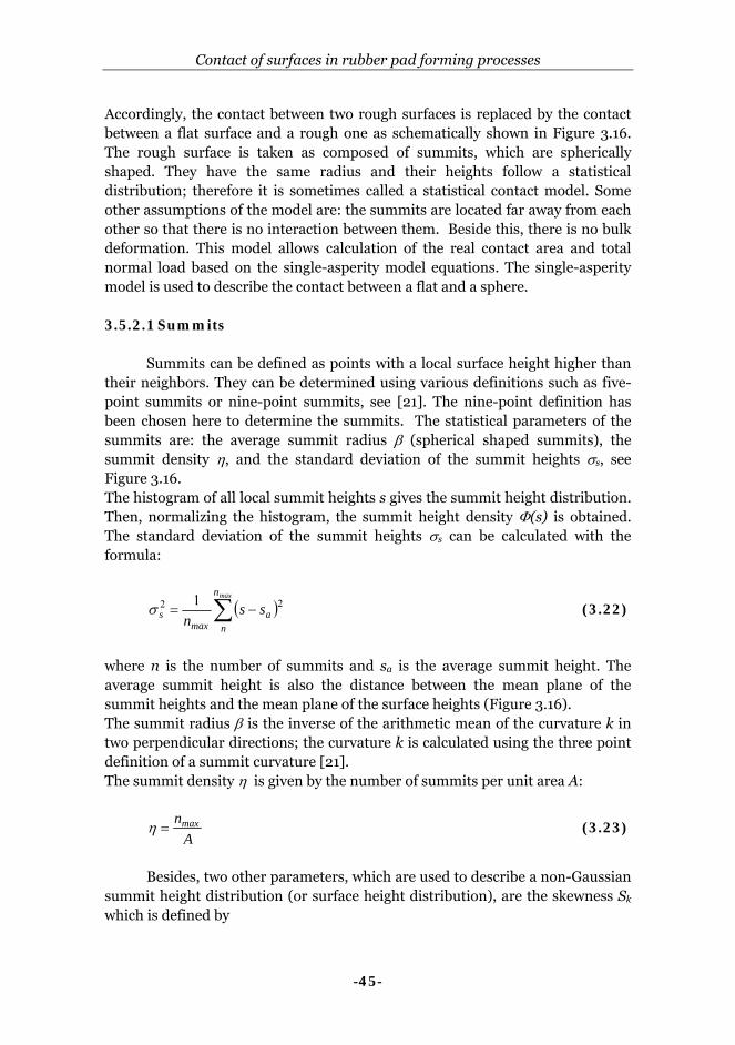
Contact of surfaces in rubber pad forming processes
-45-
Accordingly, the contact between two rough surfaces is replaced by the contact between a flat surface and a rough one as schematically shown in Figure 3.16. The rough surface is taken as composed of summits, which are spherically shaped. They have the same radius and their heights follow a statistical distribution; therefore it is sometimes called a statistical contact model. Some other assumptions of the model are: the summits are located far away from each other so that there is no interaction between them. Beside this, there is no bulk deformation. This model allows calculation of the real contact area and total normal load based on the single-asperity model equations. The single-asperity model is used to describe the contact between a flat and a sphere. 3.5.2.1 Summits
Summits can be defined as points with a local surface height higher than their neighbors. They can be determined using various definitions such as five-point summits or nine-point summits, see [21]. The nine-point definition has been chosen here to determine the summits. The statistical parameters of the summits are: the average summit radius β (spherical shaped summits), the summit density η, and the standard deviation of the summit heights σs, see Figure 3.16. The histogram of all local summit heights s gives the summit height distribution. Then, normalizing the histogram, the summit height density Φ(s) is obtained. The standard deviation of the summit heights σs can be calculated with the formula:
( )∑ −=maxn
na
maxs ss
n22 1σ (3.22)
where n is the number of summits and sa is the average summit height. The average summit height is also the distance between the mean plane of the summit heights and the mean plane of the surface heights (Figure 3.16). The summit radius β is the inverse of the arithmetic mean of the curvature k in two perpendicular directions; the curvature k is calculated using the three point definition of a summit curvature [21]. The summit density η is given by the number of summits per unit area A:
A
nmax=η (3.23)
Besides, two other parameters, which are used to describe a non-Gaussian
summit height distribution (or surface height distribution), are the skewness Sk which is defined by

Chapter 3
-46-
( ) ( )∫∞
∞−
⋅−= dssssS as
k φσ
33
1 (3.24)
and the kurtosis Ks given by
( ) ( )∫∞
∞−
⋅−= dssssK as
s φσ
44
1 (3.25)
The skewness Sk provides information regarding the symmetry of the height distribution. The kurtosis Ks shows how the summit heights are distributed around the average summit height sa. For instance, a Gaussian distribution has Sk = 0 and Ks = 3.
Table 3.6 Summit roughness parameters.
Material β [μm] σs [μm] η ⋅1010 [m-2]
Aluminum alloy 3.1 0.528 2.27 Polyurethane 95 Shore A 343.4 0.016 1.41 Polyurethane 90 Shore A 14.9 0.19 0.67 Polyurethane 80 Shore A 0.6 1.874 3.96
The summit parameters of the polyurethane samples and metal sheet are presented in Table 3.6. They were obtained by processing the surface roughness data obtained with the interference microscope in Matlab, according to the procedure explained in [21]. A surface with a large average summit radius and a small σs is considered smoot, while one with a small average summit radius and a high σs is taken as rough.
Fig. 3.18. Summit locations
(polyurethane). Fig.3.17. Distribution of the summits as a
function of the summit heights (polyurethane).

Contact of surfaces in rubber pad forming processes
-47-
The distribution of the summits as a function of the summit heights is plotted in Figure 3.17 for the polyurethane 80 Shore A and in Figure 3.19 for the aluminum sheet. It is clear that the summits have different radii and that the higher summits have smaller radii. The locations of all summits are shown in Figure 3.18 and 3.20. It can be observed that the polyurethane has an isotropic surface, the summits which are usually located on the surface ridges are randomly distributed, while for the aluminum surface they are oriented to a certain direction.
3.5.3 Overall contact (type II contact)
At relatively high loads the contact between elastic and stiff surfaces can
be regarded as a huge single-asperity contact due to flattening of the micro-asperities as indicated in Figure 3.15 (b). In this case it can be assumed that the nominal contact area is equal to the real contact area, thus, the contact can be modeled for instance by the Hertz theory [35]. The single-asperity contact will be in detail presented in the next chapter. 3.5.4 Multi-asperity contact (type III contact) Type III contact is not similar to a type I contact, because the contacting asperities are larger than the local maxima (summits). Besides, they will not deform independently. Moreover, bulk deformation can not be neglected. The contacting asperities for this case will be called “equivalent asperities”, see Figure 3.21.
Fig. 3.19. Distribution of the summits as a function of the summit heights (Al alloy).
Fig. 3.20. Summit locations (Al alloy).

Chapter 3
-48-
If we consider the surface height density from Figure 3.22, it can be
assumed that at large separations there are only a few asperities in contact which do not interact with each other, therefore they can be accurately described by a type I contact; at smaller separations (decreasing d) more asperities come into contact interacting and merging with their neighbors in the so-called equivalent asperity. This results in a type II contact at small separations.
An equivalent asperity is shown schematically in Figure 3.21. In calculations, the equivalent asperities are modeled by elliptical paraboloids. It is assumed that the normal contact area and the volume of the contacting part of the elliptical paraboloid and of the original microcontact are the same for reasons of load and energy equivalence. The radii in x and y directions which define the elliptical paraboloid are given in Appendix A1.
summits
equivalent asperity
Fig. 3.21. Micro-geometry: equivalent asperity and summits.
z [m]
pro
babi
lity
den
sity
Type I
Type III h
d
Fig. 3.22. Influence of surface height density on using summits or equivalent asperities, for d see Fig. 3.16.

Contact of surfaces in rubber pad forming processes
-49-
Besides replacing the summits by equivalent asperities, their interaction and the bulk deformation will be also considered. The multi-asperity contact case including the interaction of neighboring asperities will be comprehensively explained in Chapter 5.
3.6 Contact and friction between rubber pad and metal sheet Compared to other polymers the polyurethane used as a flexible tool (90-95 Shore A) is stiff. Thus, the multi-asperity contact approach appears to be suitable for the rubber-metal contact at relatively large loads, while at low loads the multi-summit approach can be appropriate. A rough estimation of the real contact area as a function of normal load could give an indication of the behavior of the coefficient of friction for different materials in contact. When rough stiff surfaces are involved, so a type I contact, the real contact area is proportional to the normal load (Ar ~ Fn) which will result in a constant coefficient of friction for a constant shear stress τ:
μ = Ff/Fn = τ⋅Ar/Fn ~ constant (3.26) At the other extreme, so a type II contact, when one of the materials in contact is soft compared to the other one, the contact is similar to that between a large (soft) asperity and a rigid one. Thus according to Hertz theory the contact area is proportional to the normal load to the power 2/3 which determines a coefficient of friction given by the following equation assuming a constant shear stress τ:
μ = Ff/Fn = τ ⋅ Ar/Fn ~ Fn2/3/Fn ~ Fn
-1/3 (3.27)
Fig. 3.23. Relation between the real contact area and friction: curve 1 –stiff rough surface, type I contact; curve 2 – soft rough surface, type II contact.
A
Fn
A~Fn
A ~ 2/3nF type I
type II
μ
Fn
type II
μ ~ -1/3nF
type I
Chapter 3
-50-
These relations are plotted in Figure 3.23. The polyurethane-metal contact is most probably located somewhere in between these limits. So, the coefficient of friction is expected to decrease with increasing normal load. A comprehensive analysis will be presented in the following chapters.
3.7 Summary and conclusions The properties of the contacting bodies in terms of mechanical properties, surface energy and roughness are described as well as the measurement techniques. Depending on the ratio of real contact area to nominal contact area, different approaches can be used to model the contact of real bodies. When the contact area is a small fraction of the nominal contact area a multi-summit model (for instance Greenwood-Williamson) is appropriate. At the other extreme, when the real contact area almost equals the nominal contact area, a single-like asperity model is suitable. The intermediate case can be modeled using a multi-asperity contact which accounts for asperity interaction and bulk deformation.

-51-
Chapter 4
Single-asperity static friction model
Introduction The normal contact between a viscoelastic sphere and a rigid flat
is modeled using a modified Hertz theory in which the viscoelastic behavior is incorporated through a mechanical model. When a tangential load is subsequently applied, a mechanism similar to that described by the Mindlin theory is assumed to take place in the contact area. At low loads adhesion starts to play an important role. Its effect has been modeled according to Johnson-Kendall-Roberts (JKR) theory, in which a factor has been included which accounts for the work of adhesion of viscoelastic materials. Friction is attributed to the shear of the interfacial layer which separates the bodies in contact. A static friction model is developed based on the above-mentioned contact models. Furthermore, a parametric study is presented regarding the influence of several parameters on the static friction force and limiting displacement.
In summary, the normal contact of elastic bodies is discussed then this case is extended to viscoelastic bodies including also adhesion effect. Afterwards, the case of tangential loading of elastic and viscoelastic bodies including adhesion is presented. Finally, the shear in the interfacial layer is modeled as well as the static friction in the contact of a viscoelastic asperity and a rigid flat.
4.1 Normal loading of elastic bodies The solution of the normal contact between two elastic spheres (see Figure 4.1) with respect to the contact radius a, normal approach (or penetration) δn and pressure distribution p(r) is given by Hertz [35]:
3/1
*43
⎟⎠⎞
⎜⎝⎛
⋅⋅⋅
=E
RFa n (4.1)
31
2*
22
169
⎟⎟⎠
⎞⎜⎜⎝
⎛
⋅==
REF
Ra n
nδ (4.2)
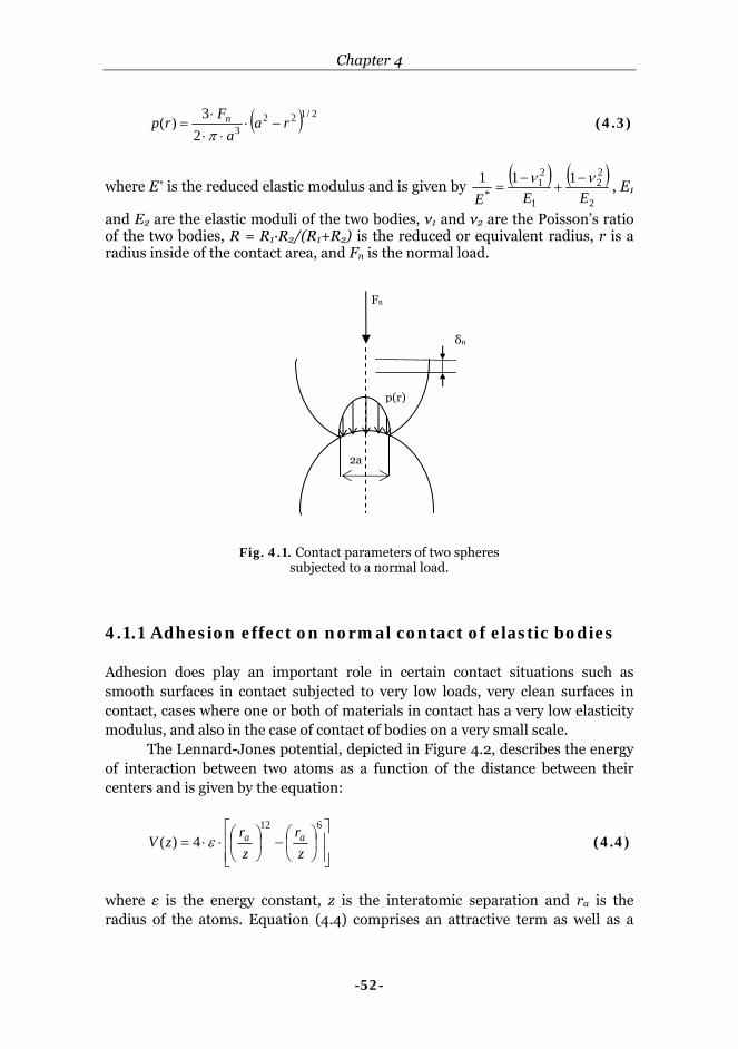
Chapter 4
-52-
( ) 2/12232
3)( raa
Frp n −⋅⋅⋅
⋅=
π (4.3)
where E* is the reduced elastic modulus and is given by ( ) ( )
2
22
1
21
*111
EEEνν −
+−
= , E1
and E2 are the elastic moduli of the two bodies, ν1 and ν2 are the Poisson’s ratio of the two bodies, R = R1·R2/(R1+R2) is the reduced or equivalent radius, r is a radius inside of the contact area, and Fn is the normal load.
4.1.1 Adhesion effect on normal contact of elastic bodies Adhesion does play an important role in certain contact situations such as smooth surfaces in contact subjected to very low loads, very clean surfaces in contact, cases where one or both of materials in contact has a very low elasticity modulus, and also in the case of contact of bodies on a very small scale.
The Lennard-Jones potential, depicted in Figure 4.2, describes the energy of interaction between two atoms as a function of the distance between their centers and is given by the equation:
⎥⎥⎦
⎤
⎢⎢⎣
⎡⎟⎠
⎞⎜⎝
⎛−⎟⎠
⎞⎜⎝
⎛⋅⋅=612
4)(zr
zr
zV aaε (4.4)
where ε is the energy constant, z is the interatomic separation and ra is the radius of the atoms. Equation (4.4) comprises an attractive term as well as a
Fig. 4.1. Contact parameters of two spheres subjected to a normal load.
δn
2a
Fn
p(r)
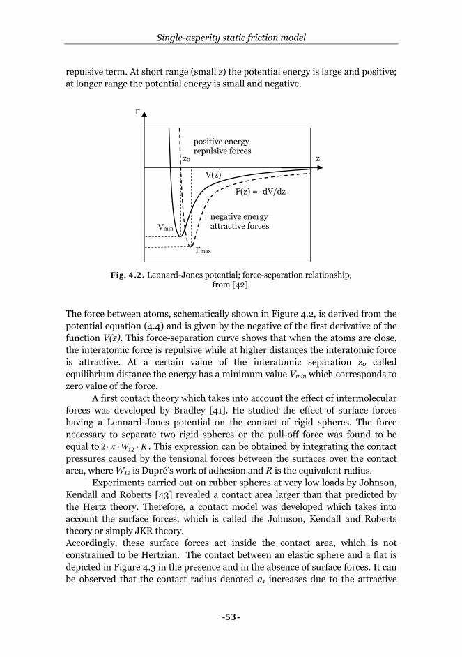
Single-asperity static friction model
-53-
repulsive term. At short range (small z) the potential energy is large and positive; at longer range the potential energy is small and negative.
The force between atoms, schematically shown in Figure 4.2, is derived from the potential equation (4.4) and is given by the negative of the first derivative of the function V(z). This force-separation curve shows that when the atoms are close, the interatomic force is repulsive while at higher distances the interatomic force is attractive. At a certain value of the interatomic separation z0 called equilibrium distance the energy has a minimum value Vmin which corresponds to zero value of the force. A first contact theory which takes into account the effect of intermolecular forces was developed by Bradley [41]. He studied the effect of surface forces having a Lennard-Jones potential on the contact of rigid spheres. The force necessary to separate two rigid spheres or the pull-off force was found to be equal to RW ⋅⋅⋅ 122 π . This expression can be obtained by integrating the contact pressures caused by the tensional forces between the surfaces over the contact area, where W12 is Dupré’s work of adhesion and R is the equivalent radius. Experiments carried out on rubber spheres at very low loads by Johnson, Kendall and Roberts [43] revealed a contact area larger than that predicted by the Hertz theory. Therefore, a contact model was developed which takes into account the surface forces, which is called the Johnson, Kendall and Roberts theory or simply JKR theory. Accordingly, these surface forces act inside the contact area, which is not constrained to be Hertzian. The contact between an elastic sphere and a flat is depicted in Figure 4.3 in the presence and in the absence of surface forces. It can be observed that the contact radius denoted a1 increases due to the attractive
Fig. 4.2. Lennard-Jones potential; force-separation relationship, from [42].
Fmax
Vmin
negative energy attractive forces
positive energy repulsive forces
V(z)
F(z) = -dV/dz
z0 z
F
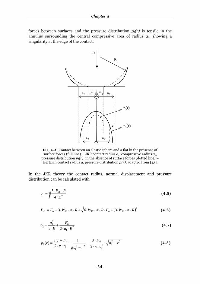
Chapter 4
-54-
forces between surfaces and the pressure distribution p1(r) is tensile in the annulus surrounding the central compressive area of radius ac, showing a singularity at the edge of the contact.
In the JKR theory the contact radius, normal displacement and pressure distribution can be calculated with
3 11
⋅4
⋅⋅3=
*ERF
a n (4.5)
( )21212121 363 RWFRWRWFF nnn ⋅⋅⋅+⋅⋅⋅⋅+⋅⋅⋅+= πππ (4.6)
*1
21
1 23 EaF
Ra n
⋅⋅+
⋅=δ (4.7)
2213
1
1
2211
11 −⋅
⋅⋅2
⋅3−
−
1⋅
⋅⋅2−
= raa
F
raaFF
rp nnn
ππ)( (4.8)
Fig. 4.3. Contact between an elastic sphere and a flat in the presence of surface forces (full line) – JKR contact radius a1, compressive radius ac,
pressure distribution p1(r); in the absence of surface forces (dotted line) – Hertzian contact radius a, pressure distribution p(r), adapted from [43].
p(r)
p1(r)
a1 a
R
Fn
a a1
ac ac
Single-asperity static friction model
-55-
where Fn1 is the apparent Hertzian load which would determine a contact radius a1. The pressure distribution p1(r) comprises a tensile zone close to the edge of the contact area and a central compressive part whose radius is given by
1
11 3
1n
nnc F
FFaa
−+⋅= (4.9)
The pull-off force found by Johnson, Kendall and Roberts [43] is equal to
RW ⋅⋅⋅ 122/3 π , so independent on the material properties like elasticity modulus and in contradiction with the force found by Bradley [41.] Derjaguin, Muller and Toporov [44] presented a different theory, called the DMT theory, using a thermodynamic approach. In the DMT model the surface forces act outside the contact area, while the geometry is limited to be Hertzian. They found that the pull-off force is equal to RW ⋅⋅⋅ 122 π (the same result as in Bradley’s theory) and there is no stress singularity at the edge of contact.
At a first sight contradictory, these theories have proved to apply to different limits of contact situations, indicated by a non-dimensional parameter introduced by Tabor [46]. This parameter can be interpreted as the ratio of the elastic deformation to the range of action of the surface forces and is given by:
3/1
30
2
212
⎟⎟⎠
⎞⎜⎜⎝
⎛
⋅
⋅=
∗ zEWR
Tμ (4.10)
where z0 is the equilibrium spacing in the Lennard-Jones potential (see Figure 4.2) and E* is the combined elastic modulus. Consequently, Bradley’s analysis and DMT theory provide a good approximation for small μT, in which case the elastic deformation is negligible. For highly adhesive systems, corresponding to large values of μT, the JKR theory is appropriate.
The intermediate regime has been studied by Maugis [45] using a Dugdale approximation for the surface forces.
In the Dugdale approximation, schematically shown in Figure 4.4, the stress is constant and equal to σ0 until a separation ho is reached and then it falls to zero. This maximum stress matches the Lennard-Jones potential, from which the separation h0 = 0.97·z0 is obtained by keeping the energy to separate the two bodies in both cases the same.

Chapter 4
-56-
In the theory of Maugis, the contact is maintained over a central region in
which the pressure is Hertzian and the constant adhesive stresses extend to a radius c (see Figure 4.5). Thus, the net or total pressure pt(r) acting on the contact area is the sum of the Hertz pressure p(r), and the adhesive tension pa(r) acting on the circle of radius c. The total force is the sum of the applied load Fn and of the adhesion force Fa.
Based on the Maugis-Dugdale intermediate model an adhesion map has been constructed by Johnson and Greenwood [47] in order to determine the
Fig. 4.5. Maugis - Dugdale distribution of surface traction: p - Hertz pressure acting on a circle of radius a; pa - the adhesive tension acting on circle of radius c, from [47].
R Fn
c
p
F0
c
g2
Fa
pt
a a
pa
Fig. 4.4. Dugdale approximation, adapted from [42].
Lennard-Jones
Dugdale
h0 = 0.97·z0
σ0
z
t
ensi
on
c
omp
ress
ion

Single-asperity static friction model
-57-
appropriate model for a certain contact situation and for a certain material couple.
The adhesion map is plotted in Figure 4.6 having on the x-coordinate the elasticity parameter given by:
TEWR μ
πσλ ⋅=⎟
⎟⎠
⎞⎜⎜⎝
⎛
⋅⋅⋅⋅
⋅= 16.12
93/1
*12
0 (4.11)
and on the y-coordinate the ratio of the net force to the adhesive pull-off force, which can be written as:
RW
FF n
n ⋅⋅=
12π (4.12)
A rough analysis done in [47] indicates that contacts involving low elasticity materials such as elastomers correspond to a Tabor parameter μT > 100, so they are located in the JKR regime of the adhesion map. In the case of materials with a high elasticity modulus the value of the Tabor parameter is typically μT < 1 which corresponds to the Bradley region.
Fig. 4.6. Adhesion map, adapted from [47].
λ = 1.16 ·μT
F n / π·
R·W
12
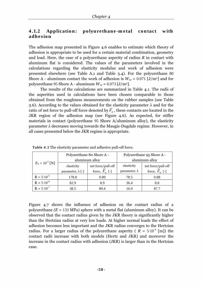
Chapter 4
-58-
4.1.2 Application: polyurethane-metal contact with adhesion The adhesion map presented in Figure 4.6 enables to estimate which theory of adhesion is appropriate to be used for a certain material combination, geometry and load. Here, the case of a polyurethane asperity of radius R in contact with aluminum flat is considered. The values of the parameters involved in the calculations regarding the elasticity modulus and work of adhesion were presented elsewhere (see Table A.1 and Table 3.4). For the polyurethane 80 Shore A - aluminum contact the work of adhesion is W12 = 0.071 [J/m2] and for polyurethane 95 Shore A - aluminum W12 = 0.073 [J/m2]. The results of the calculations are summarized in Table 4.1. The radii of the asperities used in calculations have been chosen comparable to those obtained from the roughness measurements on the rubber samples (see Table 3.6). According to the values obtained for the elasticity parameter λ and for the ratio of net force to pull-off force denoted by nF , these contacts are located in the JKR region of the adhesion map (see Figure 4.6). As expected, for stiffer materials in contact (polyurethane 95 Shore A/aluminum alloy), the elasticity parameter λ decreases moving towards the Maugis-Dugdale regime. However, in all cases presented below the JKR regime is appropriate.
Table 4.1 The elasticity parameter and adhesive pull-off force.
Polyurethane 80 Shore A -
aluminum alloy
Polyurethane 95 Shore A -
aluminum alloy Fn = 10-5 [N]
elasticity
parameter, λ [-]
net force/pull-off
force, nF [-]
elasticity
parameter, λ
net force/pull-off
force, nF [-]
R = 5·10-5 178.8 0.89 78.5 0.88 R = 5·10-6 82.9 8.9 36.4 8.8 R = 5·10-7 38.5 89.4 16.9 87.7
Figure 4.7 shows the influence of adhesion on the contact radius of a polyurethane (E = 133 MPa) sphere with a metal flat (aluminum alloy). It can be observed that the contact radius given by the JKR theory is significantly higher than the Hertzian radius at very low loads. At higher normal loads the effect of adhesion becomes less important and the JKR radius converges to the Hertzian radius. For a larger radius of the polyurethane asperity ( R = 5·10-4 [m]) the contact radii increase with both models (Hertz and JKR) and moreover the increase in the contact radius with adhesion (JKR) is larger than in the Hertzian case.

Single-asperity static friction model
-59-
The influence of elasticity modulus on the contact radius in both cases with and without adhesion is illustrated in Figure 4.8. As expected, the contact radii, i.e. Hertz theory and JKR theory, are larger for materials with a low elasticity modulus, this effect being the same for the case with adhesion and without adhesion.
4.2 Normal loading of viscoelastic-rigid asperity couple 4.2.1 Modeling the behavior of viscoelastic materials As it was already mentioned in Chapter 3.2, viscoelastic materials incorporate both elastic and viscous characteristics. This material behavior can be predicted by using purely phenomenological models, so-called mechanical models consisting of springs and dashpots connected in series and/or in parallel.
Fig. 4.7. Comparison of the contact radii without adhesion (Hertz theory) and with adhesion (JKR theory) for two radii of asperities, R = 5·10-5 and R = 5·10-4 [m].
1.E-07
1.E-06
1.E-05
1.E-04
1.E-08 1.E-07 1.E-06 1.E-05 1.E-04 1.E-03 1.E-02
Normal load [N]
Cont
act r
adiu
s [m
]
aHertz R = 5*10^-5 [m]aJKR R = 5*10^-5 [m]aHertz R = 5*10^-4 [m]aJKR R = 5*10^-4 [m]
log10
log10
Fig. 4.8. Comparison of the contact radii without adhesion (Hertz theory) and with adhesion (JKR theory) for two polyurethanes (E = 38 [MPa] and E = 133 [MPa]).
1.E-07
1.E-06
1.E-05
1.E-04
1.E-08 1.E-07 1.E-06 1.E-05 1.E-04 1.E-03 1.E-02Normal load [N]
Con
tact
radi
us [m
]
aHertz E = 38 [MPa]aJKR E = 38 [MPa]aHertz E = 133 [MPa]aJKR E = 133 [MPa]
log10
log10

Chapter 4
-60-
The simplest mechanical models comprise one spring in series or in parallel with one dashpot as shown in Figure 4.9 a-b. The Maxwell model (Figure 4.9 a) describes properly the relaxation behavior while the Voight model (Figure 4.9 b) is appropriate for creep.
The Standard Linear Solid (SLS) model gives a relatively good description of both stress relaxation and creep behavior. Usually, a combination of several Kelvin or Maxwell elements is necessary to describe accurately the behavior of real viscoelastic materials. In order to keep the contact model analytically tractable a Standard Linear Solid behavior will be used in this thesis. However, there is no restriction to extent it to more complicated material models. For the SLS model the generalized Hook’s equation can be written as: ( ) σσηεεη ⋅++⋅=⋅⋅+⋅⋅ 21211 ggggg && (4.13)
where g1, 2 is the elasticity of the springs, η is the viscosity of the dashpot, ε is the strain, and σ is the stress.
The creep compliance function φ(t) can be obtained from equation (4.13) by making the stress constant and equal to σ0 and solving the differential equation with respect to the strain ε, resulting in:
( ) ( ) ( )[ ]2210
111 T/texpgg
tt −−⋅+==σεϕ (4.14)
where T2 = η/g2 is the retardation time.
g
η
σ, ε
g η
σ, ε g1
g2 η
σ, ε
a. b. c.
Fig. 4.9. Mechanical models: a. Maxwell model; b. Kelvin (or Voight) model; c. Standard Linear Solid (or Zener) model.

Single-asperity static friction model
-61-
Similarly, the stress relaxation function can be obtained by taking the stain constant and equal to ε0 in equation (4.13) and is given by:
( ) ( ) ( )[ ]21221
1
0T/texpgg
gggtt −⋅+⋅+
==εσψ (4.15)
where T2 = η/(g1 + g2) is the relaxation time. For 0→t an instantaneous modulus E0 can be defined which is equal to
( ) ( ) 1100 g== −ϕψ and for ∞→t the relaxed modulus E∞ is given by
( ) ( )21
211
gggg
⋅+
=∞=∞ −ψϕ .
The creep compliance and stress relaxation function are input parameters of the contact model as it will be shown in the next section, therefore they have to be quantified. The stress relaxation function of the SLS model (equation 4.15) has been fitted with the experimental curve obtained from tensile measurements (as described in section 3.2.1) in order to determine the parameters of the mechanical model in terms of elasticity of the springs (g1, 2) and dashpot viscosity (η).
Figure 4.10 shows the fitted and the experimental curves for polyurethane 95 Shore A for two periods of time, 30 [s] and 180 [s] respectively. It can be observed that they fit relatively well; only at the start of the relaxation they do not mach very well. A mechanical model with more parameters (i.e. springs and dashpots) would be able to describe the behavior more closely. The values of the SLS parameters are summarized in Table 4.2. Depending on the time of the experiment, an increase of the value for the elasticity of the springs is observed for shorter periods of time, while the value of the dashpot viscosity increases for longer periods of time.
4.0E+07
4.5E+07
5.0E+07
5.5E+07
6.0E+07
6.5E+07
7.0E+07
7.5E+07
0 50 100 150 200
Time [s]
Stre
ss r
elax
atio
n m
odul
us [P
a]
measured
Standard Linear Solid
4.0E+07
4.5E+07
5.0E+07
5.5E+07
6.0E+07
6.5E+07
7.0E+07
7.5E+07
0 5 10 15 20 25 30
Time [s]
Stre
ss r
elax
atio
n m
odul
us [P
a] measured
Standard Linear Solid
Fig. 4.10. Measured (polyurethane 95 Shore A) and curve fitted (Standard Linear Solid) stress relaxation modulus vs. time: left – 30 [s], right – 180 [s].

Chapter 4
-62-
Table 4.2 Standard Linear Solid parameters.
SLS parameters
polyurethane 95 Shore A g1 [N/m2] g2 [N/m2] η [N⋅s/m2]
t = 30 [s] 6.43⋅107 2.34⋅108 1.49⋅109
t = 180 [s] 5.77⋅107 2.13⋅108 7.95⋅109
4.2.2 Normal loading of viscoelastic-rigid asperity couple The Hertz theory was extended by Lee and Radok [7] to linear viscoelastic bodies using the correspondence principle. According to this principle the solution to a viscoelastic problem can be obtained from the elastic solution. The case of normal contact between a linear viscoelastic asperity and a rigid one is presented by Johnson in [6]. A Standard Linear Solid model was chosen to describe the viscoelastic behavior of rubber-like material in terms of both creep and relaxation (see Figure 4.9. c). The elastic sphere was assumed to be incompressible (ν = 0.5) with a shear modulus G. The viscoelastic solution is presented for two cases: when the variation of penetration is prescribed (displacement-controlled case) and when the load variation is given (load-controlled case). In the displacement controlled case a certain variation of normal displacement δn = δn(t) is imposed, then the contact radius, pressure distribution and normal load are given by [6]:
( ) ( )[ ] 21 /n tRta δ⋅= (4.16)
( ) ( )[ ]∫ ′−′′
⋅′−⋅⋅
=t
/tdrta
tddtt
R)t,r(p
0
21224 ψπ
(4.17)
( ) ( )∫0
3 ′′′
⋅′−⋅⋅38
=t
n tdtatddtt
RtF ψ)( (4.18)
In the load-controlled case, the variation of the normal load is given Fn = Fn(t) and the following relations result for the contact area and pressure distribution [6]:
( ) ( )∫ ′′′
⋅′−⋅⋅=t
tdtPtd
dttR)t(a0
3
83 ϕ (4.19)

Single-asperity static friction model
-63-
( )[ ]∫ ′−′′
⋅′−
⋅⋅
=t
/tdrta
tdd
)tt(R)t,r(p
0
212214ϕπ
(4.20)
In order to keep the calculations analytically tractable, in the following sections the normal load (load-controlled case) or normal displacement (displacement-controlled case) will be taken as Heaviside step functions. The simplified equations for such a case, written for a viscoelastic-rigid asperity couple are presented in Appendix B, equations B.1 to B.8. Results obtained with the equations showed above will be presented in section 4.2.3.2. First, the effect of adhesion on the contact parameters for a viscoelastic-rigid couple will be discussed. 4.2.3 Adhesion effect on the normal contact of a viscoelastic-rigid couple 4.2.3.1 Viscoelastic contact with adhesion – theoretical background The adhesive contact between viscoelastic bodies has been studied by Maugis & Barquins [49] using the fracture mechanics theory, due to the similarities between the crack propagation in a body and the receding or the advancing contact area between two bodies, as shown schematically in Figure 4.11.
For elastic bodies in contact subjected to either compressive or tensile forces, the equilibrium is given by the Griffith’s criterion:
Fig. 4.11. The similarity between the receding contact area of two spheres subjected to tensile loads and the crack propagation in a body.
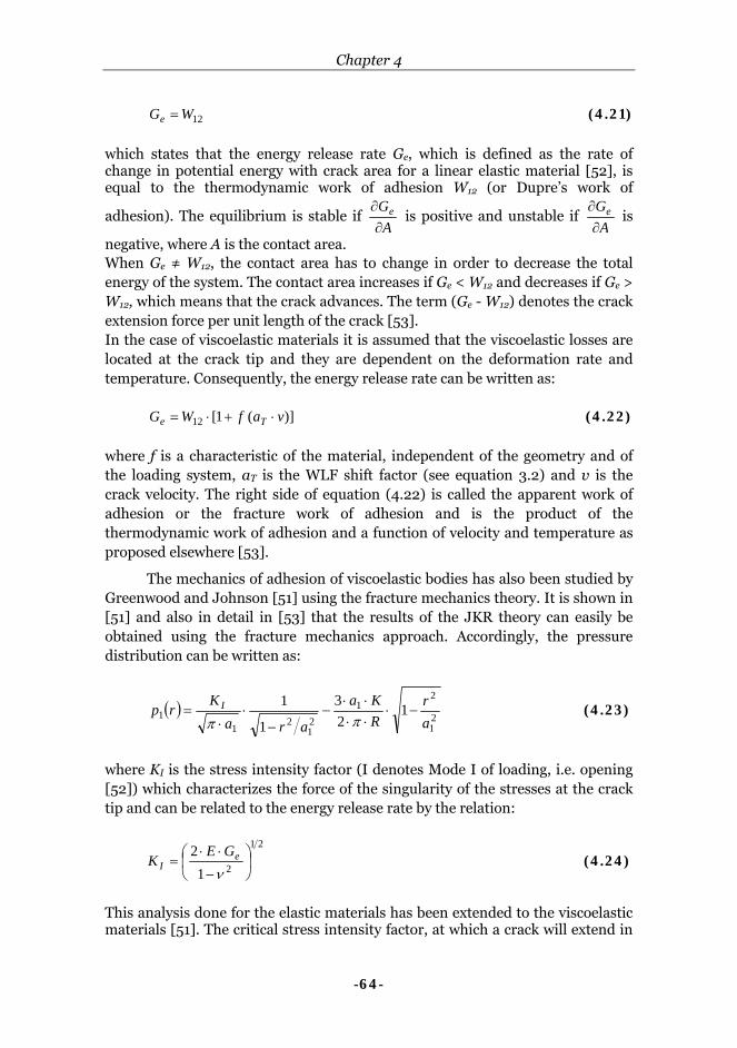
Chapter 4
-64-
12WGe = (4.21)
which states that the energy release rate Ge, which is defined as the rate of change in potential energy with crack area for a linear elastic material [52], is equal to the thermodynamic work of adhesion W12 (or Dupre’s work of
adhesion). The equilibrium is stable if A
Ge
∂∂
is positive and unstable if A
Ge
∂∂
is
negative, where A is the contact area. When Ge ≠ W12, the contact area has to change in order to decrease the total energy of the system. The contact area increases if Ge < W12 and decreases if Ge > W12, which means that the crack advances. The term (Ge - W12) denotes the crack extension force per unit length of the crack [53]. In the case of viscoelastic materials it is assumed that the viscoelastic losses are located at the crack tip and they are dependent on the deformation rate and temperature. Consequently, the energy release rate can be written as:
)](1[12 vafWG Te ⋅+⋅= (4.22)
where f is a characteristic of the material, independent of the geometry and of the loading system, aT is the WLF shift factor (see equation 3.2) and v is the crack velocity. The right side of equation (4.22) is called the apparent work of adhesion or the fracture work of adhesion and is the product of the thermodynamic work of adhesion and a function of velocity and temperature as proposed elsewhere [53].
The mechanics of adhesion of viscoelastic bodies has also been studied by Greenwood and Johnson [51] using the fracture mechanics theory. It is shown in [51] and also in detail in [53] that the results of the JKR theory can easily be obtained using the fracture mechanics approach. Accordingly, the pressure distribution can be written as:
( ) 21
21
21
21
1 123
1
1ar
RKa
araKrp I −⋅
⋅⋅⋅⋅
−−
⋅⋅
=ππ
(4.23)
where KI is the stress intensity factor (I denotes Mode I of loading, i.e. opening [52]) which characterizes the force of the singularity of the stresses at the crack tip and can be related to the energy release rate by the relation:
21
212
⎟⎠
⎞⎜⎝
⎛−
⋅⋅=
νe
IGE
K (4.24)
This analysis done for the elastic materials has been extended to the viscoelastic materials [51]. The critical stress intensity factor, at which a crack will extend in

Single-asperity static friction model
-65-
an elastic material, defined in [51] as π2I
cKN = has been analyzed for the
loading and unloading of viscoelastic bodies. It was assumed that the bodies separate similarly to the shape of the Griffith’s crack depicted in Figure 4.12 a.
Due to the viscoelastic dissipation within the material, the loading case (increasing contact area) has to be treated separately from the unloading case (decreasing contact area). It has been found that the same equation applies in the viscoelastic case for the critical stress intensity factor as in the elastic case, in which the instantaneous modulus E0 is used instead of the elastic modulus. For the loading case the work of adhesion is scaled by a viscoelastic factor *
*0
∞
=EE
kv and is given by:
v
v kWW 12= (4.25)
while in the unloading case the effective work of adhesion is vkW ⋅12 . The viscoelastic factor is independent of the separation rate, which seems to be in discrepancy with some experimental results presented in [49]. However, when a step load or displacement is applied to a material couple, it is expected that the rate of separation to have a minor effect. The loading rate has been considered in a more complex analysis [51] developed for a Barenblatt crack (see Figure 4.12 b).
An adhesion theory has been developed by Hui, Baney and Kramer [50] for the contact of viscoelastic spheres based on the Maugis-Dugdale [45] adhesion model. In their theory the mechanics of the viscoelastic contact, the so called outer problem, has been coupled with the local micromechanics of adhesion or the inner problem as shown in Figure 4.13.
Fig. 4.12. The shape and the stress distribution at the tip of a) a conventional Griffith crack and b) according to Barenblatt, from [51].
a) b)
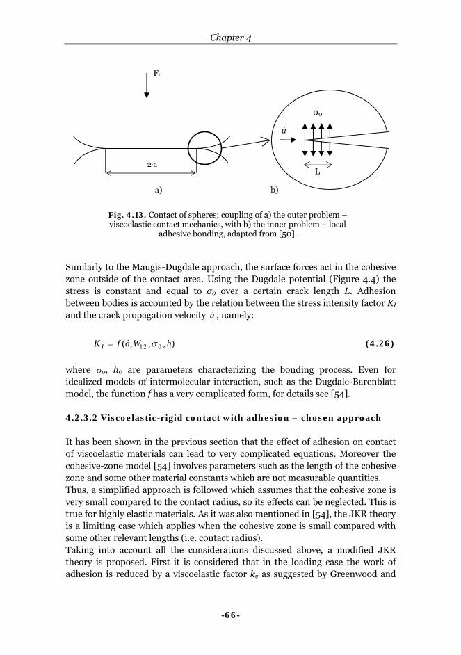
Chapter 4
-66-
Similarly to the Maugis-Dugdale approach, the surface forces act in the cohesive zone outside of the contact area. Using the Dugdale potential (Figure 4.4) the stress is constant and equal to σ0 over a certain crack length L. Adhesion between bodies is accounted by the relation between the stress intensity factor KI and the crack propagation velocity a& , namely:
),,,( hWafK I 012= σ& (4.26)
where σ0, h0 are parameters characterizing the bonding process. Even for idealized models of intermolecular interaction, such as the Dugdale-Barenblatt model, the function f has a very complicated form, for details see [54]. 4.2.3.2 Viscoelastic-rigid contact with adhesion – chosen approach It has been shown in the previous section that the effect of adhesion on contact of viscoelastic materials can lead to very complicated equations. Moreover the cohesive-zone model [54] involves parameters such as the length of the cohesive zone and some other material constants which are not measurable quantities. Thus, a simplified approach is followed which assumes that the cohesive zone is very small compared to the contact radius, so its effects can be neglected. This is true for highly elastic materials. As it was also mentioned in [54], the JKR theory is a limiting case which applies when the cohesive zone is small compared with some other relevant lengths (i.e. contact radius). Taking into account all the considerations discussed above, a modified JKR theory is proposed. First it is considered that in the loading case the work of adhesion is reduced by a viscoelastic factor kv as suggested by Greenwood and
L
σ0
a&
Fn
2·a
Fig. 4.13. Contact of spheres; coupling of a) the outer problem – viscoelastic contact mechanics, with b) the inner problem – local
adhesive bonding, adapted from [50].
a) b)

Single-asperity static friction model
-67-
Johnson in [51]. The modified equations written for a viscoelastic-rigid couple are presented in Appendix B, equations (B.9) to (B.12). As showed in Figure 4.3, the JKR distribution of pressure p1(r) comprises a central compressive part and an annular tensile part in which the surfaces tend to peel apart. In this approach, in order to be able to apply the Mindlin approach and to calculate the static friction force, it is considered that only the compressive part has a significant contribution in the contact. It is noticed that the shape of the compressive part almost resembles a Hertzian pressure distribution. Thus, the compressive pressure distribution has been fitted with a Hertzian distribution denoted pe(r) by keeping the load equivalence. The equivalent Herzian pressure distribution is written as
( ) ( ) ( ) 224, rtatR
trp cve
e −⋅⋅⋅
=φπ
(4.27)
where acv is the radius of the contact area under compression, see equation (B.12) in Appendix B, and Re is the reduced equivalent radius deduced from the load equivalence condition as
( ) ( )
( ) ( ) ( ) ( ) ( )( ) ( ) ⎥⎦⎤
⎢⎣⎡ ⋅+⋅−⋅⋅−⋅
⋅⋅
38
=31
211
2221
31
3
nvnvncvcvv
vcve
FtaFtaFtatatat
tataR
ϕ (4.28)
with a1v and Fn1 given by equations (B.9) and (B.10) in Appendix B. The contact of a viscoelastic asperity with a rigid flat has been chosen to illustrate the theory proposed above. The input parameters used in the calculations are summarized in Table 4.3.
Table 4.3 Values of the input parameters.
Parameter Symbol Value Unit
Work of adhesion Wv 0.34 mJ/m2
Elasticity of the spring (SLS model) g1 6.43⋅107 [N/m2]
Elasticity of the spring (SLS model) g2 2.34⋅108 [N/m2]
Viscosity of the dashpot (SLS model) η 1.49⋅109 [N⋅s/m2]
Radius of the sphere R 5⋅10-5 [m]
The distribution of pressure in the contact area is shown in Figure 4.14 for three contact situations at a certain time instant (t = 50 s) and for an applied normal load Fn of 10-5 [N]: first, when adhesion is not taken into account, the distribution of pressure pv(r) is calculated with equation (B.4) from Appendix B;
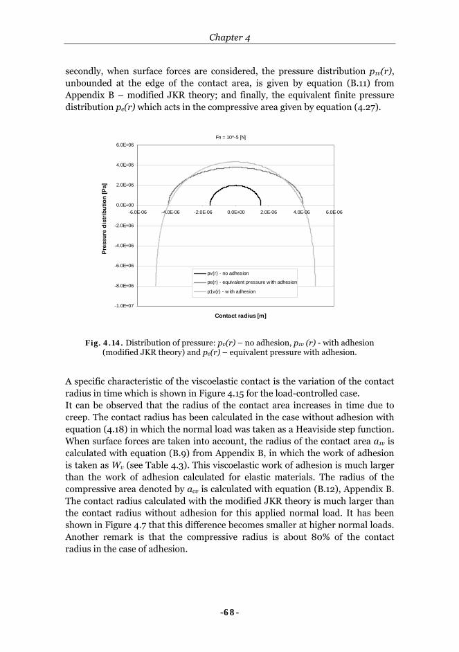
Chapter 4
-68-
secondly, when surface forces are considered, the pressure distribution p1v(r), unbounded at the edge of the contact area, is given by equation (B.11) from Appendix B – modified JKR theory; and finally, the equivalent finite pressure distribution pe(r) which acts in the compressive area given by equation (4.27).
A specific characteristic of the viscoelastic contact is the variation of the contact radius in time which is shown in Figure 4.15 for the load-controlled case. It can be observed that the radius of the contact area increases in time due to creep. The contact radius has been calculated in the case without adhesion with equation (4.18) in which the normal load was taken as a Heaviside step function. When surface forces are taken into account, the radius of the contact area a1v is calculated with equation (B.9) from Appendix B, in which the work of adhesion is taken as Wv (see Table 4.3). This viscoelastic work of adhesion is much larger than the work of adhesion calculated for elastic materials. The radius of the compressive area denoted by acv is calculated with equation (B.12), Appendix B. The contact radius calculated with the modified JKR theory is much larger than the contact radius without adhesion for this applied normal load. It has been shown in Figure 4.7 that this difference becomes smaller at higher normal loads. Another remark is that the compressive radius is about 80% of the contact radius in the case of adhesion.
Fig. 4.14. Distribution of pressure: pv(r) – no adhesion, p1v (r) - with adhesion (modified JKR theory) and pe(r) – equivalent pressure with adhesion.
Fn = 10^-5 [N]
-1.0E+07
-8.0E+06
-6.0E+06
-4.0E+06
-2.0E+06
0.0E+00
2.0E+06
4.0E+06
6.0E+06
-6.0E-06 -4.0E-06 -2.0E-06 0.0E+00 2.0E-06 4.0E-06 6.0E-06
Contact radius [m]
Pre
ssur
e di
stri
butio
n [P
a]
pv(r) - no adhesion
pe(r) - equivalent pressure w ith adhesion
p1v(r) - w ith adhesion

Single-asperity static friction model
-69-
In summary, this approach, suitable for viscoelastic materials, predicts a contact radius larger than that obtained in the elastic case with JKR theory (for comparison see Figure 4.7); a Hertzian type pressure distribution is obtained by taking the contact area equal to that under compression and by keeping the load equivalence. It will be shown later in this chapter that this Hertzian pressure distribution allows us to model static friction for viscoelastic-rigid contacts using a similar theory to that developed by Mindlin for elastic materials.
4.3 Tangential loading of elastic bodies Now, an elastic sphere is considered which is normally and tangentially loaded against a rigid by the compressive load Fn and tangential load Ft (see Figure 4.16). If the tangential force Ft is less than the force needed to cause macrosliding, it is firstly assumed that the bodies will deform in shear without any slip at the interface. The contact area and pressure distribution are caused by the normal load (Hertz theory) and are not influenced by the tangential load. Thus, the shear stress distribution which produces a uniform tangential displacement of a circular contact area is given in [18] by:
21
2
2
0 1)(−
⎟⎟⎠
⎞⎜⎜⎝
⎛−⋅=
arr ττ (4.29)
where 20 2 aFt ⋅⋅= πτ . This relation is schematically shown in Figure 4.17,
curve A. It can be observed that it has a singularity at the r = a, which means that the shear stress increases theoretically to infinite at the edge of the contact.
Fig. 4.15. Radius of the contact area vs. time without adhesion (Hertz), with adhesion (modified JKR), and radius of the
compressive area.
Fn = 10^-5 [N]
1.0E-06
1.5E-06
2.0E-06
2.5E-06
3.0E-06
3.5E-06
4.0E-06
4.5E-06
5.0E-06
5.5E-06
0 5 10 15 20 25Time [s]
Con
tact
rad
ius
[m]
Hertz theorymodified JKR theorycompressive radius
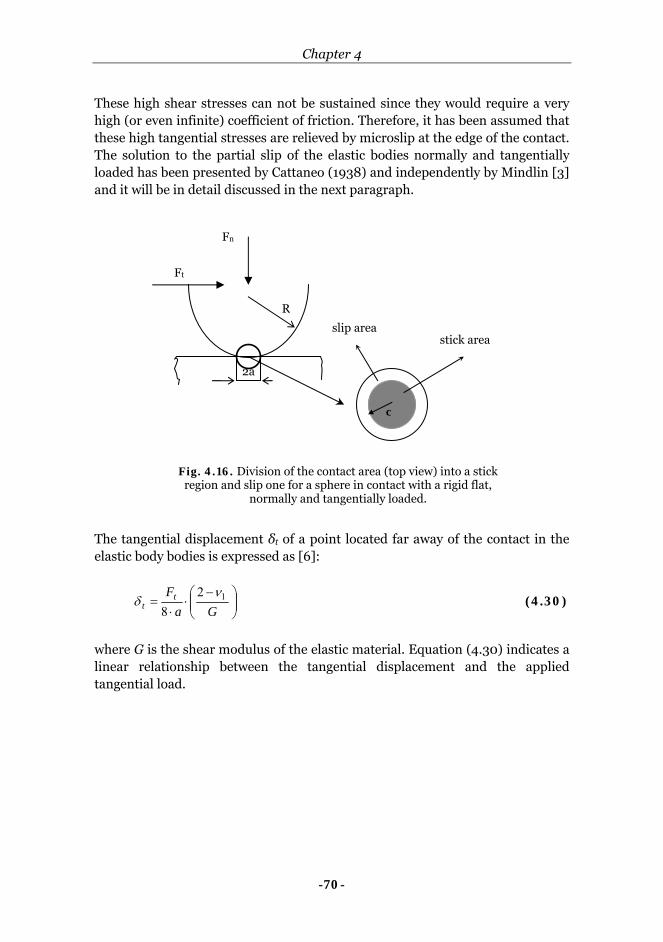
Chapter 4
-70-
These high shear stresses can not be sustained since they would require a very high (or even infinite) coefficient of friction. Therefore, it has been assumed that these high tangential stresses are relieved by microslip at the edge of the contact. The solution to the partial slip of the elastic bodies normally and tangentially loaded has been presented by Cattaneo (1938) and independently by Mindlin [3] and it will be in detail discussed in the next paragraph.
The tangential displacement δt of a point located far away of the contact in the elastic body bodies is expressed as [6]:
⎟⎟⎠
⎞⎜⎜⎝
⎛ −2⋅
⋅8= 1
GaFt
tν
δ (4.30)
where G is the shear modulus of the elastic material. Equation (4.30) indicates a linear relationship between the tangential displacement and the applied tangential load.
Fn
Ft
R
2a
stick area slip area
c
Fig. 4.16. Division of the contact area (top view) into a stick region and slip one for a sphere in contact with a rigid flat,
normally and tangentially loaded.
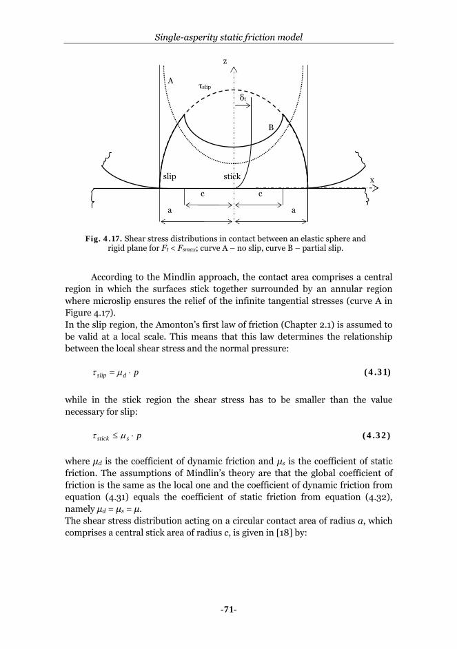
Single-asperity static friction model
-71-
According to the Mindlin approach, the contact area comprises a central region in which the surfaces stick together surrounded by an annular region where microslip ensures the relief of the infinite tangential stresses (curve A in Figure 4.17). In the slip region, the Amonton’s first law of friction (Chapter 2.1) is assumed to be valid at a local scale. This means that this law determines the relationship between the local shear stress and the normal pressure: pdslip ⋅= μτ (4.31)
while in the stick region the shear stress has to be smaller than the value necessary for slip: psstick ⋅≤ μτ (4.32)
where μd is the coefficient of dynamic friction and μs is the coefficient of static friction. The assumptions of Mindlin’s theory are that the global coefficient of friction is the same as the local one and the coefficient of dynamic friction from equation (4.31) equals the coefficient of static friction from equation (4.32), namely μd = μs = μ. The shear stress distribution acting on a circular contact area of radius a, which comprises a central stick area of radius c, is given in [18] by:
Fig. 4.17. Shear stress distributions in contact between an elastic sphere and rigid plane for Ft < Fsmax; curve A – no slip, curve B – partial slip.
a a
c c
B
τslip
z
stick x
δt
slip
A
Chapter 4
-72-
( )
( ) ( )⎪⎪⎩
⎪⎪⎨
⎧
≤≤⎥⎦⎤
⎢⎣⎡ −−−⋅
⋅⋅⋅⋅
≤≤−⋅⋅⋅
⋅⋅=
stick 02
3
slip 2
3)(
2/1222/1223
2/1223
crifrcraa
F
arcifraa
F
rn
n
πμ
πμ
τ (4.33)
and is depicted in Figure 4.17, curve B. The shear stress in the slip area is written for the moment when the two surfaces in contact are on the point of sliding, thus, the coefficient of static friction μs is used. By integrating the shear stresses over the contact area, the magnitude of the tangential load Ft is obtained. From this, the radius c of the stick circle is deduced:
3/1
1 ⎟⎟⎠
⎞⎜⎜⎝
⎛⋅
−⋅=n
t
FFac
μ (4.34)
The magnitude of the slip at a radius r inside of the slip region and the relative tangential displacement of the two bodies were found by Johnson [6] to be:
( )⎥⎥
⎦
⎤
⎢⎢
⎣
⎡
⎟⎟⎠
⎞⎜⎜⎝
⎛−⋅⋅+⎟
⎟⎠
⎞⎜⎜⎝
⎛⋅−⋅⎟
⎠⎞
⎜⎝⎛ ⋅−⋅−⋅
⋅⋅⋅⋅
= −2/1
2
2
2
21 1221sin212
323
)(rc
rc
rc
rc
GaF
rs nt ππ
νμ
(4.35)
⎥⎥
⎦
⎤
⎢⎢
⎣
⎡⎟⎟⎠
⎞⎜⎜⎝
⎛⋅
−−⋅⎟⎠⎞
⎜⎝⎛ −⋅
⋅⋅⋅
=3/2
11216
3
n
tnt F
FGa
Fμ
νμδ (4.36)
4.4 Tangential loading of a viscoelastic-rigid couple In order to keep the proposed model analytically tractable, as explained before it is assumed that the applied load and displacement are Heaviside step functions. Similarly to the normal contact, the solution to the tangential loaded contact of viscoelastic bodies is obtained from the elastic solution by substituting the elastic constant with the appropriate viscoelastic operators. It is also assumed that the contact area between a viscoelastic sphere and a rigid flat does not change its circularity during the tangential loading. Both particular cases, load-controlled and displacement-controlled are presented below.
Load-controlled case A viscoelastic sphere is considered which is pressed against a rigid flat by a normal load that varies in time according to:
Single-asperity static friction model
-73-
( ) ( )tHFtF nn ⋅= (4.37) where t is the time and H(t) is the Heaviside step function or the unit step function defined as:
⎩⎨⎧
>
==
010tfor0
)(tfor
tH (4.38)
For t > 0 the contact radius av can be written as:
( ) ( )3
83 tFR
ta nv
ϕ⋅⋅⋅= (4.39)
and the pressure distribution is expressed as:
( ) ( ) ( )22
322 )(
231)(4, rta
taF
trta
Rtrp v
v
nvv −⋅
⋅⋅
⋅=⋅−⋅
⋅=
πϕπ (4.40)
Then, the shear stress distribution is obtained as:
( )( )( ) ( ) ( )
( )( )( ) ( )( ) ( )
⎪⎪⎩
⎪⎪⎨
⎧
≤≤⎥⎦⎤
⎢⎣⎡ −−−⋅
⋅⋅⋅⋅
≤≤−⋅⋅⋅
⋅⋅
=stick t0
23
slip t2
3
),(2/1222/122
3
2/1223
vvvv
n
vvvv
n
v
crifrtcrtata
F
artcifrtata
F
tr
πμ
πμ
τ
(4.41) with the radius of the stick circle equal to:
( ) ( )3/1
1 ⎟⎟⎠
⎞⎜⎜⎝
⎛⋅
−⋅=n
tvv F
Ftatcμ
(4.42)
Similarly, by substituting the viscoelastic parameters into equations (4.35) and (4.36) the expressions for the slip at the interface sv and the tangential displacement δv are obtained:
( ) ( ) ( ) ( ) ( ) ( )⎥⎥
⎦
⎤
⎢⎢
⎣
⎡
⎟⎟⎠
⎞⎜⎜⎝
⎛−⋅⋅+⎟
⎟⎠
⎞⎜⎜⎝
⎛⋅−⋅⎟
⎠⎞
⎜⎝⎛ ⋅−⋅−⋅
⋅⋅⋅⋅
= −2/1
2
2
2
21 1221sin212
163),(
rtc
rtc
rtc
rtc
atFtrs vvvv
v
nv ππ
νϕμ
(4.43)

Chapter 4
-74-
( ) ( )( ) ( )
⎥⎥
⎦
⎤
⎢⎢
⎣
⎡⎟⎟⎠
⎞⎜⎜⎝
⎛⋅
−−⋅−⋅⋅
⋅⋅⋅=
3/2
1128
3
n
t
v
nv F
Fta
tFtμ
νϕμδ (4.44)
Displacement-controlled case In a displacement-controlled case, the normal displacement or indentation is taken as ( ) ( )tHt nn ⋅= δδ (4.45)
In this case the contact radius is constant and equal to:
[ ] 2/1nv Ra δ⋅= (4.46)
while the pressure distribution and normal load changes in time according to:
( ) 224),( ratR
trp vv −⋅⋅⋅
= ψπ
(4.47)
( ) 3
38)( vatR
tP ⋅⋅⋅
= ψ (4.48)
Equations (4.41) and (4.42) expressing the shear stress distribution and the radius of the stick zone apply also to the displacement-controlled case together with the equations (4.46), (4.47) and (4.48). The slip at the interface and the tangential displacement of points far away from the contact are obtained from equations (4.43) and (4.44) by replacing the creep compliance function φ(t) with the relaxation function ψ(t). 4.4.1 Application: viscoelastic-rigid contact The theory presented in the previous section is applied now to a polyurethane/rigid material couple subjected to a constant normal load (load-controlled case) and subsequently to an increasing tangential load, up to the point of sliding. Some input parameters are given in Table 4.4 and the parameters of the mechanical model are given in Table 4.3. A constant coefficient of static friction is assumed and the tangential load is taken as an increasing function of time Ft(t) = t·10-7. Having set these input parameters, the shear stress distribution inside the contact area can be determined.
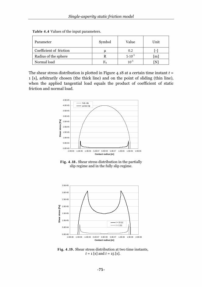
Single-asperity static friction model
-75-
Table 4.4 Values of the input parameters.
Parameter Symbol Value Unit
Coefficient of friction μ 0.2 [-]
Radius of the sphere R 5⋅10-5 [m]
Normal load Fn 10-5 [N]
The shear stress distribution is plotted in Figure 4.18 at a certain time instant t = 1 [s], arbitrarily chosen (the thick line) and on the point of sliding (thin line), when the applied tangential load equals the product of coefficient of static friction and normal load.
Fig. 4.18. Shear stress distribution in the partially slip regime and in the fully slip regime.
0.0E+00
5.0E+04
1.0E+05
1.5E+05
2.0E+05
2.5E+05
3.0E+05
3.5E+05
4.0E+05
4.5E+05
-2.0E-06 -1.5E-06 -1.0E-06 -5.0E-07 0.0E+00 5.0E-07 1.0E-06 1.5E-06 2.0E-06
Contact radius [m]
Shea
r st
ress
[Pa]
fully slip partial slip
0.0E+00
5.0E+04
1.0E+05
1.5E+05
2.0E+05
2.5E+05
3.0E+05
3.5E+05
-2.0E-06 -1.5E-06 -1.0E-06 -5.0E-07 0.0E+00 5.0E-07 1.0E-06 1.5E-06 2.0E-06
Contact radius [m]
Shea
r st
ress
[Pa]
t = 15 [s]t = 1 [s]
Fig. 4.19. Shear stress distribution at two time instants, t = 1 [s] and t = 15 [s].
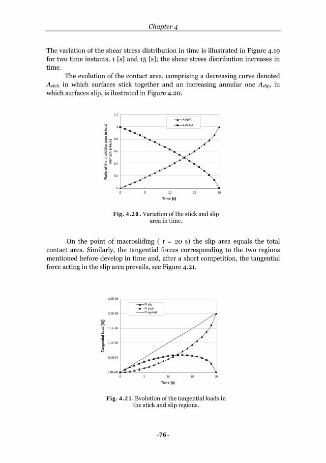
Chapter 4
-76-
The variation of the shear stress distribution in time is illustrated in Figure 4.19 for two time instants, 1 [s] and 15 [s]; the shear stress distribution increases in time.
The evolution of the contact area, comprising a decreasing curve denoted Astick in which surfaces stick together and an increasing annular one Aslip, in which surfaces slip, is ilustrated in Figure 4.20.
On the point of macrosliding ( t = 20 s) the slip area equals the total
contact area. Similarly, the tangential forces corresponding to the two regions mentioned before develop in time and, after a short competition, the tangential force acting in the slip area prevails, see Figure 4.21.
Fig. 4.20. Variation of the stick and slip area in time.
0
0.2
0.4
0.6
0.8
1
1.2
0 5 10 15 20
Time [s]
Ratio
of t
he s
tick/
slip
are
a to
tota
l co
ntac
t are
a [-]
Aslip/A
Astick/A
Fig. 4.21. Evolution of the tangential loads in the stick and slip regions.
0.0E+00
5.0E-07
1.0E-06
1.5E-06
2.0E-06
2.5E-06
0 5 10 15 20
Time [s]
Tang
entia
l loa
d [N
]]
Ft slipFt stickFt applied

Single-asperity static friction model
-77-
The dependence of the tangential displacement on the applied tangential load is shown in Figure 4.22 for two normal loads, the other input parameters being kept the same. Both parameters as well as their maximum values before macrosliding increase with normal load, the shape of the graph showing the same almost linear part at start followed by a non-linear part close to the moment of sliding.
4.4.1.1 Viscoelastic-rigid contact with adhesion The approach proposed in section 4.2.3.2 for normal contact of a viscoelastic material and a rigid one will be used to study the tangential loading of the same couple of materials when adhesion is taken into account. The contact area as well as the contact pressure increase when the surface forces are taken into account. The equations used to calculate the parameters of the contact in the case with adhesion are presented in Appendix B, equation (B.9) to (B.12). The coefficient of friction is calculated as the ratio of the tangential load necessary to initiate sliding to the total normal load over the compressive area, i.e. the sum of the normal applied load and the force due to adhesion:
an
slidingt
FFF
+=μ (4.49)
A polyurethane sphere is normally loaded (Heaviside step load) against a rigid flat and subsequently a tangential force Ft(t) = t·10-7 is applied. The input parameters used in the calculations are the same as those given in Table 4.3 and Table 4.4.
Fig. 4.22. Tangential load vs. tangential displacement for two normal loads Fn, 10-5 and 10-4 [N].
0.E+00
5.E-06
1.E-05
2.E-05
2.E-05
3.E-05
0.E+00 1.E-08 2.E-08 3.E-08 4.E-08 5.E-08 6.E-08 7.E-08
Tangential displacement [m]
Tang
entia
l loa
d [N
]
Fn = 10^-5 [N]
Fn = 10^-4 [N]
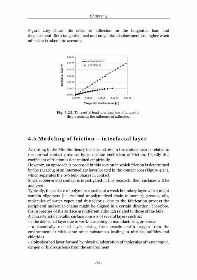
Chapter 4
-78-
Figure 4.23 shows the effect of adhesion on the tangential load and displacement. Both tangential load and tangential displacement are higher when adhesion is taken into account.
4.5 Modeling of friction – interfacial layer According to the Mindlin theory the shear stress in the contact area is related to the normal contact pressure by a constant coefficient of friction. Usually this coefficient of friction is determined empirically. However, an approach is proposed in this section in which friction is determined by the shearing of an intermediate layer located in the contact area (Figure 4.24), which separates the two bulk phases in contact. Since rubber-metal contact is investigated in this research, their surfaces will be analyzed. Typically, the surface of polymers consists of a weak boundary layer which might contain oligomers (i.e. residual unpolymerized chain monomer), greases, oils, molecules of water vapor and dust/debris; due to the fabrication process the peripheral molecular chains might be aligned in a certain direction. Therefore, the properties of the surface are different although related to those of the bulk. A characteristic metallic surface consists of several layers such as: - a the deformed layer due to work-hardening in manufacturing processes - a chemically reacted layer arising from reaction with oxygen from the environment or with some other substances leading to nitrides, sulfides and chlorides - a physisorbed layer formed by physical adsorption of molecules of water vapor, oxygen or hydrocarbons from the environment
Fig. 4.23. Tangential load as a function of tangential displacement; the influence of adhesion.
0.0E+00
2.0E-06
4.0E-06
6.0E-06
8.0E-06
1.0E-05
1.2E-05
0.0E+00 5.0E-09 1.0E-08 1.5E-08 2.0E-08
Tangential displacement [m]
Tang
entia
l loa
d [N
]w ithout adhesion
w ith adhesion
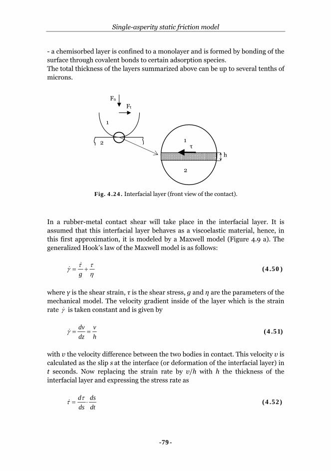
Single-asperity static friction model
-79-
- a chemisorbed layer is confined to a monolayer and is formed by bonding of the surface through covalent bonds to certain adsorption species. The total thickness of the layers summarized above can be up to several tenths of microns.
In a rubber-metal contact shear will take place in the interfacial layer. It is assumed that this interfacial layer behaves as a viscoelastic material, hence, in this first approximation, it is modeled by a Maxwell model (Figure 4.9 a). The generalized Hook’s law of the Maxwell model is as follows:
ηττγ +=
g&
& (4.50)
where γ is the shear strain, τ is the shear stress, g and η are the parameters of the mechanical model. The velocity gradient inside of the layer which is the strain rate γ& is taken constant and is given by
hv
dzdv
==γ& (4.51)
with v the velocity difference between the two bodies in contact. This velocity v is calculated as the slip s at the interface (or deformation of the interfacial layer) in t seconds. Now replacing the strain rate by v/h with h the thickness of the interfacial layer and expressing the stress rate as
dtds
dsd
⋅=ττ& (4.52)
Fig. 4.24. Interfacial layer (front view of the contact).
h
τ
Fn
Ft
1
2 1
2
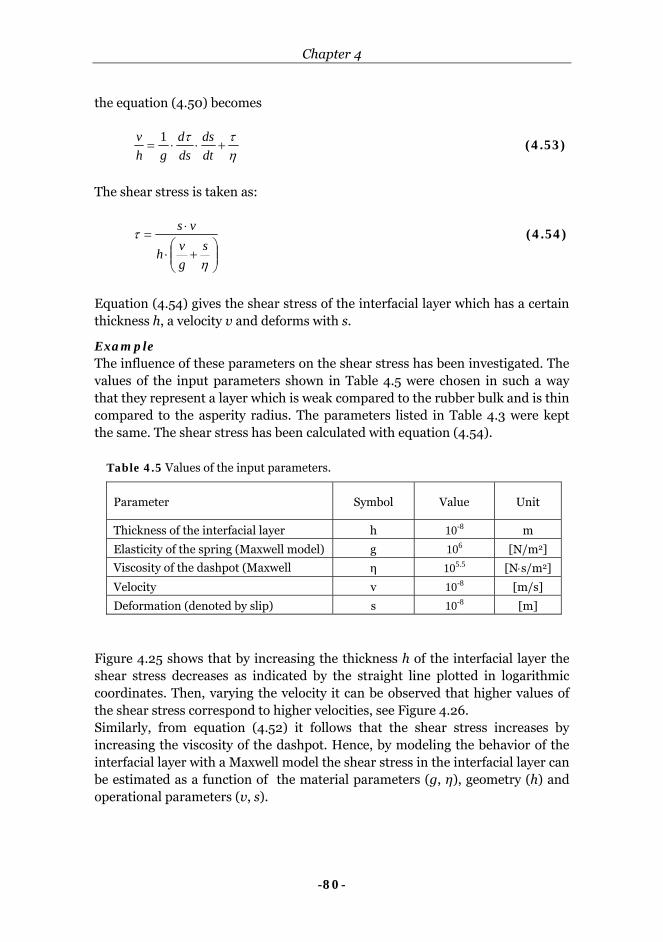
Chapter 4
-80-
the equation (4.50) becomes
ηττ
+⋅⋅=dtds
dsd
ghv 1
(4.53)
The shear stress is taken as:
⎟⎟⎠
⎞⎜⎜⎝
⎛+⋅
⋅=
η
τs
gvh
vs (4.54)
Equation (4.54) gives the shear stress of the interfacial layer which has a certain thickness h, a velocity v and deforms with s.
Example The influence of these parameters on the shear stress has been investigated. The values of the input parameters shown in Table 4.5 were chosen in such a way that they represent a layer which is weak compared to the rubber bulk and is thin compared to the asperity radius. The parameters listed in Table 4.3 were kept the same. The shear stress has been calculated with equation (4.54).
Table 4.5 Values of the input parameters.
Parameter Symbol Value Unit
Thickness of the interfacial layer h 10-8 m
Elasticity of the spring (Maxwell model) g 106 [N/m2]
Viscosity of the dashpot (Maxwell η 105.5 [N⋅s/m2]
Velocity v 10-8 [m/s]
Deformation (denoted by slip) s 10-8 [m]
Figure 4.25 shows that by increasing the thickness h of the interfacial layer the shear stress decreases as indicated by the straight line plotted in logarithmic coordinates. Then, varying the velocity it can be observed that higher values of the shear stress correspond to higher velocities, see Figure 4.26. Similarly, from equation (4.52) it follows that the shear stress increases by increasing the viscosity of the dashpot. Hence, by modeling the behavior of the interfacial layer with a Maxwell model the shear stress in the interfacial layer can be estimated as a function of the material parameters (g, η), geometry (h) and operational parameters (v, s).
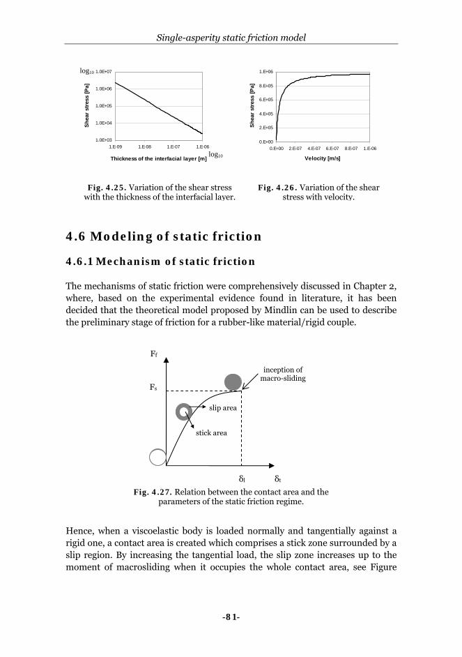
Single-asperity static friction model
-81-
4.6 Modeling of static friction 4.6.1 Mechanism of static friction The mechanisms of static friction were comprehensively discussed in Chapter 2, where, based on the experimental evidence found in literature, it has been decided that the theoretical model proposed by Mindlin can be used to describe the preliminary stage of friction for a rubber-like material/rigid couple.
Hence, when a viscoelastic body is loaded normally and tangentially against a rigid one, a contact area is created which comprises a stick zone surrounded by a slip region. By increasing the tangential load, the slip zone increases up to the moment of macrosliding when it occupies the whole contact area, see Figure
0.E+00
2.E+05
4.E+05
6.E+05
8.E+05
1.E+06
0.E+00 2.E-07 4.E-07 6.E-07 8.E-07 1.E-06
Velocity [m/s]
She
ar s
tress
[Pa]
Fig. 4.26. Variation of the shear stress with velocity.
1.0E+03
1.0E+04
1.0E+05
1.0E+06
1.0E+07
1.E-09 1.E-08 1.E-07 1.E-06
Thickness of the interfacial layer [m]
Shea
r stre
ss [P
a]
Fig. 4.25. Variation of the shear stress with the thickness of the interfacial layer.
log10
log10
Fig. 4.27. Relation between the contact area and the parameters of the static friction regime.
δl
inception of macro-sliding
δt
Ff
stick area
slip area
Fs
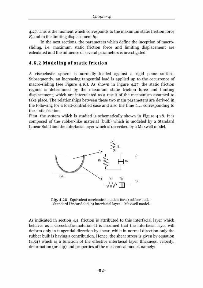
Chapter 4
-82-
4.27. This is the moment which corresponds to the maximum static friction force Fs and to the limiting displacement δl. In the next sections, the parameters which define the inception of macro-sliding, i.e. maximum static friction force and limiting displacement are calculated and the influence of several parameters is investigated. 4.6.2 Modeling of static friction A viscoelastic sphere is normally loaded against a rigid plane surface. Subsequently, an increasing tangential load is applied up to the occurrence of macro-sliding (see Figure 4.16). As shown in Figure 4.27, the static friction regime is determined by the maximum static friction force and limiting displacement, which are interrelated as a result of the mechanism assumed to take place. The relationships between these two main parameters are derived in the following for a load-controlled case and also the time tmax corresponding to the static friction. First, the system which is studied is schematically shown in Figure 4.28. It is composed of the rubber-like material (bulk) which is modeled by a Standard Linear Solid and the interfacial layer which is described by a Maxwell model.
As indicated in section 4.4, friction is attributed to this interfacial layer which behaves as a viscoelastic material. It is assumed that the interfacial layer will deform only in tangential direction by shear, while in normal direction only the rubber bulk is having a contribution. Hence, the shear stress is given by equation (4.54) which is a function of the effective interfacial layer thickness, velocity, deformation (or slip) and properties of the mechanical model, namely:
Fig. 4.28. Equivalent mechanical models for a) rubber bulk – Standard Linear Solid, b) interfacial layer – Maxwell model.
rigid g3 η2
g1
η1
a)
b)
g2
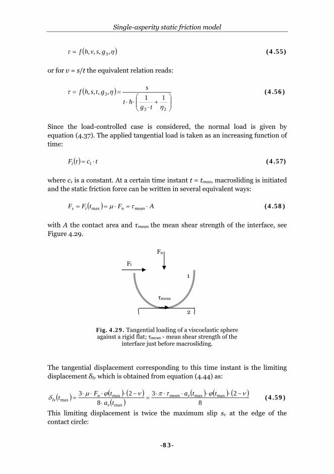
Single-asperity static friction model
-83-
( )ητ ,,,, 3gsvhf= (4.55)
or for v = s/t the equivalent relation reads:
( )⎟⎟⎠
⎞⎜⎜⎝
⎛+
⋅⋅⋅
==
23
3 11,,,,
η
ητ
tght
sgtshf (4.56)
Since the load-controlled case is considered, the normal load is given by equation (4.37). The applied tangential load is taken as an increasing function of time: ( ) tctFt ⋅= 1 (4.57)
where c1 is a constant. At a certain time instant t = tmax, macrosliding is initiated and the static friction force can be written in several equivalent ways: ( ) AFtFF meannts ⋅=⋅== τμmax (4.58)
with A the contact area and τmean the mean shear strength of the interface, see Figure 4.29.
The tangential displacement corresponding to this time instant is the limiting displacement δlv which is obtained from equation (4.44) as:
( ) ( ) ( )( )
( ) ( ) ( )8
238
23 maxmax
max
maxmax
νϕτπνϕμδ −⋅⋅⋅⋅⋅=
⋅−⋅⋅⋅⋅
=tta
tatFt vmean
v
nlv (4.59)
This limiting displacement is twice the maximum slip sv at the edge of the contact circle:
τmean
Fn
Ft
1
2
Fig. 4.29. Tangential loading of a viscoelastic sphere against a rigid flat; τmean - mean shear strength of the
interface just before macrosliding.
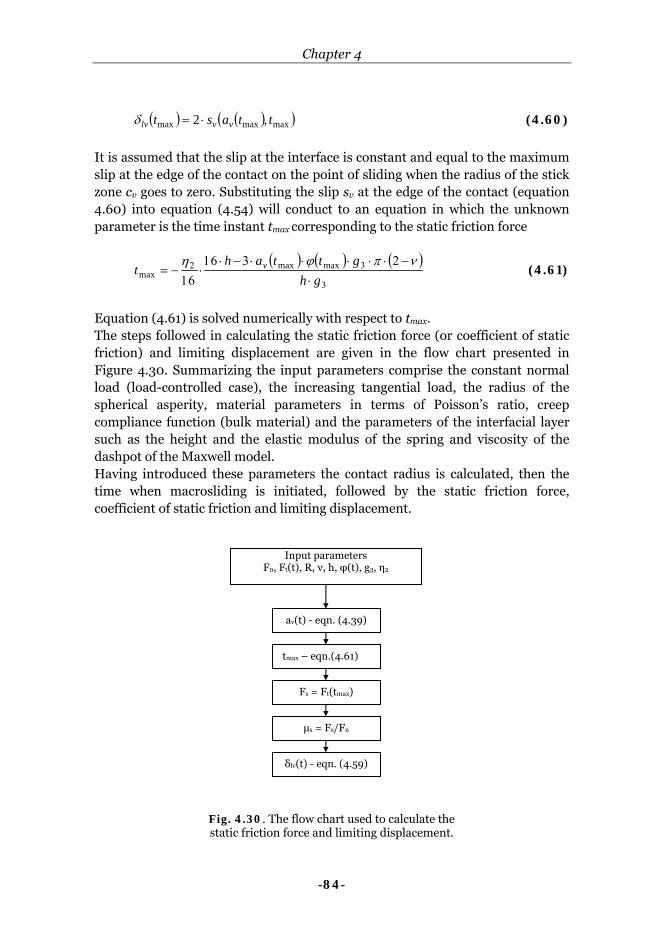
Chapter 4
-84-
( ) ( )( )maxmaxmax ,2 ttast vvlv ⋅=δ (4.60)
It is assumed that the slip at the interface is constant and equal to the maximum slip at the edge of the contact on the point of sliding when the radius of the stick zone cv goes to zero. Substituting the slip sv at the edge of the contact (equation 4.60) into equation (4.54) will conduct to an equation in which the unknown parameter is the time instant tmax corresponding to the static friction force
( ) ( ) ( )
3
32
⋅−2⋅⋅⋅⋅⋅3−⋅16
⋅16
−=gh
gttaht v νπϕη maxmax
max (4.61)
Equation (4.61) is solved numerically with respect to tmax. The steps followed in calculating the static friction force (or coefficient of static friction) and limiting displacement are given in the flow chart presented in Figure 4.30. Summarizing the input parameters comprise the constant normal load (load-controlled case), the increasing tangential load, the radius of the spherical asperity, material parameters in terms of Poisson’s ratio, creep compliance function (bulk material) and the parameters of the interfacial layer such as the height and the elastic modulus of the spring and viscosity of the dashpot of the Maxwell model. Having introduced these parameters the contact radius is calculated, then the time when macrosliding is initiated, followed by the static friction force, coefficient of static friction and limiting displacement.
Input parameters Fn, Ft(t), R, ν, h, φ(t), g3, η2
av(t) - eqn. (4.39)
tmax – eqn.(4.61)
Fs = Ft(tmax)
μs = Fs/Fn
δlv(t) - eqn. (4.59)
Fig. 4.30. The flow chart used to calculate the static friction force and limiting displacement.

Single-asperity static friction model
-85-
4.6.3 Parametric study In this section, the influence of several parameters without adhesion on the static friction force and limiting displacement is investigated. Since the coefficient of static friction is usually used in practice its dependence on various parameters is also presented. Example 1 Influence of normal load on the static friction force and limiting displacement Before discussing asperity contacts, a macroscopic example will be presented. When carrying out single-asperity friction measurements, the asperity, which is taken as a sphere, is usually scaled up. By way of example a sphere with radius R = 2 [mm] is considered. The rest of the input parameters used in calculations are listed in Table 4.6.
Table 4.6 Values of the input parameters.
Parameter Symbol Value Unit
Applied tangential load Ft Ft = 10-3.5⋅t1.5 [N]
Radius of the sphere R 2⋅10-3 [m]
Thickness of the interfacial layer h 2⋅10-7 [m]
Elasticity of the spring (SLS model) g1 6.4⋅107 [N/m2]
Elasticity of the spring (SLS model) g2 2.3⋅108 [N/m2]
Viscosity of the dashpot (SLS model) η1 1.5⋅109 [N⋅s/m2]
Elasticity of the spring (Maxwell g3 107 [N/m2]
Viscosity of the dashpot (Maxwell η2 106 [N⋅s/m2]
0.0E+00
5.0E-03
1.0E-02
1.5E-02
2.0E-02
2.5E-02
3.0E-02
3.5E-02
1.0E-07
3.0E-07
5.0E-07
7.0E-07
9.0E-07
1.1E-06
1.3E-06
1.5E-06
Limiting displacement [m]
Stat
ic fr
ictio
n fo
rce
[N]
R = 2*10^-3 [m]
0.01 0.05
0.1 0.2
0.50.7
1
Fn[N]
Fig. 4.31. Static friction force vs. limiting displacement at different normal loads.

Chapter 4
-86-
The results of the calculations done for different values of the normal load are shown in Figure 4.31 and 4.32. The pressure range (maximum pressure) for the set of loads taken in the calculations is from 2 to 9 [MPa]. It can be observed that the static friction force and limiting displacement increase by increasing the normal load. Conversely, the coefficient of static friction decreases at higher normal loads (Figure 4.32). Although both the static friction force and normal load increase it seems that the increase of normal load is prevailing.
Influence of material parameters on static friction force and limiting displacement The material behavior has been modeled by a Standard Linear Solid (see Figure 4.9 c). The parameters of the mechanical model are the elasticity of the springs g1 and g2 and the viscosity of the dashpot η. In a load-controlled case, which is the contact situation considered in the calculations, the creep compliance function ϕ(t) given by equation (4.14) describes the material behavior. For a linear viscoelastic material with the Possoins’s ratio 0.5, the shear modulus G = E/3 = 1/2⋅ϕ(t). The Standard Linear Solid model resembles the behavior of a solid-like material, therefore an increase in the elasticity of the springs g1 and g2 will lead to a decrease in the creep compliance function ϕ(t), which means an increase in the elasticity modulus E of the material (stiffer material). Due to the solid-like behavior of the mechanical model a change in the viscosity of the dashpot slightly influences the creep compliance function. Figure 4.33 shows the variation of the static friction force with the elasticity modulus of the spring g1 for a normal load of 1 [N].
0
0.05
0.1
0.15
0.2
0.25
0 0.2 0.4 0.6 0.8 1
Normal load [N]
Coef
ficie
nt o
f sta
tic fr
ictio
n [-] R = 2*10^-3 [m]
Fig. 4.32. Variation of the coefficient of static friction with normal load.
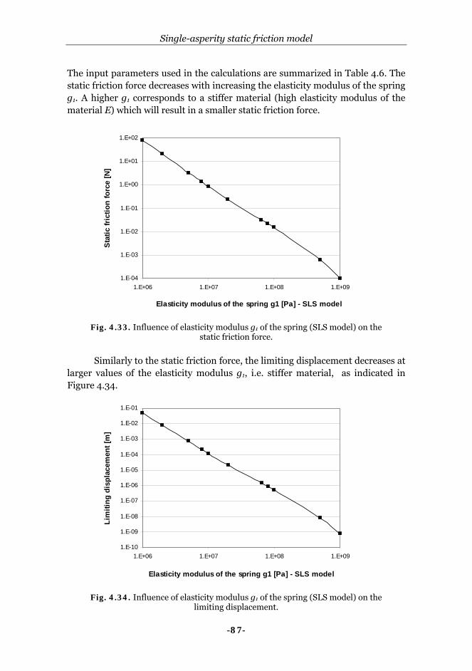
Single-asperity static friction model
-87-
The input parameters used in the calculations are summarized in Table 4.6. The static friction force decreases with increasing the elasticity modulus of the spring g1. A higher g1 corresponds to a stiffer material (high elasticity modulus of the material E) which will result in a smaller static friction force.
Similarly to the static friction force, the limiting displacement decreases at
larger values of the elasticity modulus g1, i.e. stiffer material, as indicated in Figure 4.34.
1.E-04
1.E-03
1.E-02
1.E-01
1.E+00
1.E+01
1.E+02
1.E+06 1.E+07 1.E+08 1.E+09
Elasticity modulus of the spring g1 [Pa] - SLS model
Stat
ic fr
ictio
n fo
rce
[N]
Fig. 4.33. Influence of elasticity modulus g1 of the spring (SLS model) on the
static friction force.
Fig. 4.34. Influence of elasticity modulus g1 of the spring (SLS model) on the limiting displacement.
1.E-10
1.E-09
1.E-08
1.E-07
1.E-06
1.E-05
1.E-04
1.E-03
1.E-02
1.E-01
1.E+06 1.E+07 1.E+08 1.E+09
Elasticity modulus of the spring g1 [Pa] - SLS model
Lim
iting
dis
plac
emen
t [m
]
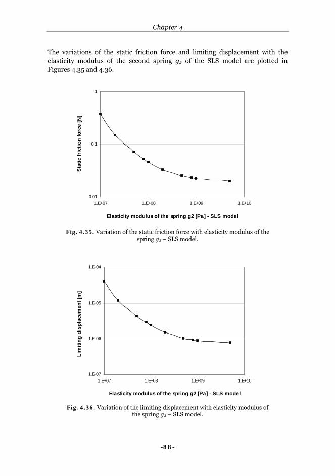
Chapter 4
-88-
The variations of the static friction force and limiting displacement with the elasticity modulus of the second spring g2 of the SLS model are plotted in Figures 4.35 and 4.36.
0.01
0.1
1
1.E+07 1.E+08 1.E+09 1.E+10
Elasticity modulus of the spring g2 [Pa] - SLS model
Stat
ic fr
ictio
n fo
rce
[N]
Fig. 4.35. Variation of the static friction force with elasticity modulus of the
spring g2 – SLS model.
Fig. 4.36. Variation of the limiting displacement with elasticity modulus of the spring g2 – SLS model.
1.E-07
1.E-06
1.E-05
1.E-04
1.E+07 1.E+08 1.E+09 1.E+10
Elasticity modulus of the spring g2 [Pa] - SLS model
Lim
iting
dis
plac
emen
t [m
]
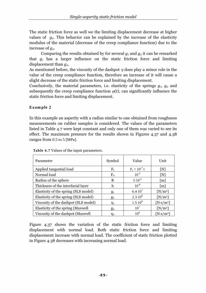
Single-asperity static friction model
-89-
The static friction force as well we the limiting displacement decrease at higher values of g2. This behavior can be explained by the increase of the elasticity modulus of the material (decrease of the creep compliance function) due to the increase of g2.
Comparing the results obtained by for several g1 and g2 it can be remarked that g1 has a larger influence on the static friction force and limiting displacement than g2. As mentioned before, the viscosity of the dashpot η does play a minor role in the value of the creep compliance function, therefore an increase of it will cause a slight decrease of the static friction force and limiting displacement. Conclusively, the material parameters, i.e. elasticity of the springs g1, g2 and subsequently the creep compliance function ϕ(t), can significantly influence the static friction force and limiting displacement. Example 2 In this example an asperity with a radius similar to one obtained from roughness measurements on rubber samples is considered. The values of the parameters listed in Table 4.7 were kept constant and only one of them was varied to see its effect. The maximum pressure for the results shown in Figures 4.37 and 4.38 ranges from 0.5 to 5 [MPa].
Table 4.7 Values of the input parameters.
Parameter Symbol Value Unit
Applied tangential load Ft Ft = 10-7⋅t [N]
Normal load Fn 10-5 [N]
Radius of the sphere R 5⋅10-5 [m]
Thickness of the interfacial layer h 10-8 [m]
Elasticity of the spring (SLS model) g1 6.4⋅107 [N/m2]
Elasticity of the spring (SLS model) g2 2.3⋅108 [N/m2]
Viscosity of the dashpot (SLS model) η1 1.5⋅109 [N⋅s/m2]
Elasticity of the spring (Maxwell g3 107 [N/m2]
Viscosity of the dashpot (Maxwell η2 106 [N⋅s/m2]
Figure 4.37 shows the variation of the static friction force and limiting displacement with normal load. Both static friction force and limiting displacement increase with normal load. The coefficient of static friction plotted in Figure 4.38 decreases with increasing normal load.

Chapter 4
-90-
Then, the thickness of the interfacial layer was varied and the rest of the input parameters were kept constant. As shown in Figure 4.25, the shear stress decreases by increasing the thickness of the interfacial layer at constant normal load. As a consequence, the static friction force as well as the limiting displacement decrease for higher values of the thickness of the interfacial layer; they are plotted in Figure 4.39. The thickness of the interfacial layer is of large influence on the coefficient of static friction, see Figure 4.40. The coefficient of static friction decreases significantly for thicker interfacial layers.
0
0.1
0.2
0.3
0.4
0.5
0.6
0.7
0.8
0.9
1
1.E-08 1.E-07 1.E-06 1.E-05 1.E-04
Normal load [N]
Coe
ffici
ent o
f sta
tic fr
ictio
n [-]
Fig. 4.38. Dependence of coefficient of
static friction on normal load. Fig. 4.37. Dependence of static friction force
and limiting displacement on normal load.
R = 5*10^-5 [m]
0.E+00
1.E-07
2.E-07
3.E-07
4.E-07
5.E-07
6.E-07
6.0E-10 8.0E-10 1.0E-09 1.2E-09 1.4E-09 1.6E-09
Limiting displacement [m]
Sta
tic fr
ictio
n fo
rce
[N]
10-8 10-7 10-6
10-5
10-4
Fn[N]
Fig. 4.39. Variation of the static friction force and limiting displacement with the thickness h
of the interfacial layer.
0.0E+00
5.0E-07
1.0E-06
1.5E-06
2.0E-06
2.5E-06
3.0E-06
0.E+00 5.E-09 1.E-08 2.E-08 2.E-08
Limiting displacement [m]
Sta
tic fr
ictio
n fo
rce
[N]
10-9
5·10-9
10-8
5·10-8
h[m]
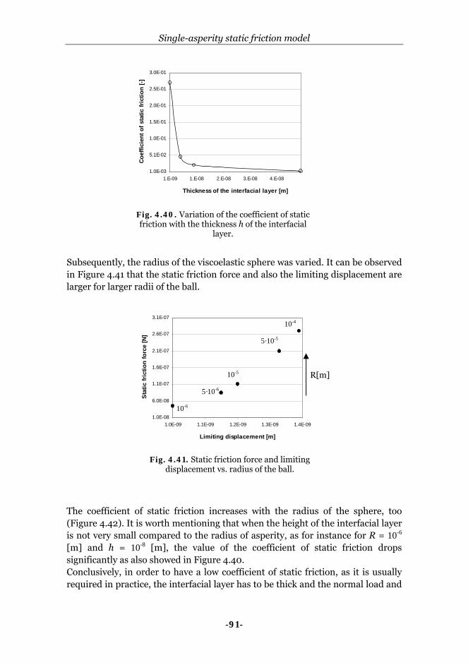
Single-asperity static friction model
-91-
Subsequently, the radius of the viscoelastic sphere was varied. It can be observed in Figure 4.41 that the static friction force and also the limiting displacement are larger for larger radii of the ball.
The coefficient of static friction increases with the radius of the sphere, too (Figure 4.42). It is worth mentioning that when the height of the interfacial layer is not very small compared to the radius of asperity, as for instance for R = 10-6 [m] and h = 10-8 [m], the value of the coefficient of static friction drops significantly as also showed in Figure 4.40. Conclusively, in order to have a low coefficient of static friction, as it is usually required in practice, the interfacial layer has to be thick and the normal load and
Fig. 4.40. Variation of the coefficient of static friction with the thickness h of the interfacial
layer.
1.0E-03
5.1E-02
1.0E-01
1.5E-01
2.0E-01
2.5E-01
3.0E-01
1.E-09 1.E-08 2.E-08 3.E-08 4.E-08
Thickness of the interfacial layer [m]
Coef
ficie
nt o
f sta
tic fr
ictio
n [-]
Fig. 4.41. Static friction force and limiting displacement vs. radius of the ball.
1.0E-08
6.0E-08
1.1E-07
1.6E-07
2.1E-07
2.6E-07
3.1E-07
1.0E-09 1.1E-09 1.2E-09 1.3E-09 1.4E-09
Limiting displacement [m]
Sta
tic fr
ictio
n fo
rce
[N]
10-6
5·10-6
10-5
5·10-5
10-4
R[m]

Chapter 4
-92-
the radius of the asperity have to be small. The same conditions are required also for smaller limiting displacements.
4.6.4. Adhesion effect on the single-asperity static friction model The approach proposed in section 4.2.3.2, for the contact with adhesion between a viscoelastic asperity and a rigid flat, is used in the single-asperity static friction model when surface forces are taken into account. It has been shown that due to the surface forces acting inside of the contact area, the apparent normal load increases, as well as the radius of the contact circle. The algorithm presented in Figure 4.30 applies also in the case with adhesion; the radius of the contact area av(t) is replaced by the radius of the contact area including surface forces acv(t) (see equation B.12 in Appendix B) and the total normal load is Fn1 which is calculated with equation (B.10) from Appendix B. The input parameters used in calculations are the same as those from Table 4.3 regarding Wv and Table 4.7 with respect to Fn, Ft(t), R, ν, h, φ(t), g3, η2. The pressure range in the case without adhesion for the loads indicated in Figure 4.43 is from 0.2 to 5 [MPa], while in the case with adhesion the pressure range increases taking values from 4.3 to 5.6 [MPa]. This increase in the pressure range in adhesive contacts is due to the increase in the total normal load which for the input parameters considered is larger than the increase in the contact area.
Fig. 4.42. Coefficient of static friction force vs. radius of the ball.
1.0E-03
6.0E-03
1.1E-02
1.6E-02
2.1E-02
2.6E-02
3.1E-02
1.E-06 1.E-05 1.E-04Radius [m]
Coef
ficie
nt o
f sta
tic fr
ictio
n [-]
log10
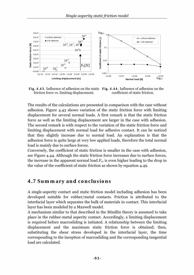
Single-asperity static friction model
-93-
The results of the calculations are presented in comparison with the case without adhesion. Figure 4.43 shows variation of the static friction force with limiting displacement for several normal loads. A first remark is that the static friction force as well as the limiting displacement are larger in the case with adhesion. The second remark is with respect to the variation of the static friction force and limiting displacement with normal load for adhesive contact. It can be noticed that they slightly increase due to normal load. An explanation is that the adhesion force is quite large at very low applied loads, therefore the total normal load is mainly due to surface forces. Conversely, the coefficient of static friction is smaller in the case with adhesion, see Figure 4.44. Although the static friction force increases due to surface forces, the increase in the apparent normal load Fn1 is even higher leading to the drop in the value of the coefficient of static friction as shown by equation 4.49.
4.7 Summary and conclusions A single-asperity contact and static friction model including adhesion has been developed suitable for rubber/metal contacts. Friction is attributed to the interfacial layer which separates the bulk of materials in contact. This interfacial layer has been modeled by a Maxwell model. A mechanism similar to that described in the Mindlin theory is assumed to take place in the rubber-metal asperity contact. Accordingly, a limiting displacement is required before macrosliding is initiated. A relationship between the limiting displacement and the maximum static friction force is obtained; then, substituting the shear stress developed in the interfacial layer, the time corresponding to the inception of macrosliding and the corresponding tangential load are calculated.
Fig. 4.43. Influence of adhesion on the static friction force vs. limiting displacement.
0.E+00
1.E-07
2.E-07
3.E-07
4.E-07
5.E-07
6.E-07
7.E-07
8.E-07
9.E-07
5.E-10 7.E-10 9.E-10 1.E-09 1.E-09 2.E-09 2.E-09 2.E-09
Limiting displacement [m]
Stat
ic fr
ictio
n fo
rce
[N]
w ithout adhesion
w ith adhesion
Fn[N] 10-8 10-7
10-610-5
10-4
10-4
10-5
10-8, 10-7, 10-6
0.001
0.01
0.1
1
1.E-08 1.E-07 1.E-06 1.E-05 1.E-04
Normal load [N]
Coef
ficie
nt o
f sta
tic fr
ictio
n [-] w ithout adhesion
w ith adhesion
Fig. 4.44. Influence of adhesion on the
coefficient of static friction.
log10
log10
Chapter 4
-94-
At low loads adhesion plays a significant role. Therefore it has been modeled by a modified JKR theory which takes into account the viscoelastic behavior of rubber. A parametric study is presented regarding the influence of several parameters such as normal load, material parameters, geometry (radius of the sphere), height of the interfacial layer on the static friction force (coefficient of static friction) and preliminary displacement. A scale effect in terms of the radius of asperity has been observed. The coefficient of static friction decreases significantly for very small radii of asperities. The results of calculations show that in order to have a smaller coefficient of static friction the normal load has to be increased, the radius of asperity has to be smaller or the interfacial layer should be thicker.

-95-
Chapter 5
Multi-asperity static friction model
Introduction In Chapter 3 it has been shown that surface roughness plays a
significant role in the contact and friction between surfaces. A few approaches used to model the surface roughness have been discussed and the main parameters which describe the surface roughness have been introduced. Then, in Chapter 4 a single-asperity static friction model for a viscoelastic-rigid contact has been developed. In this chapter, the single-asperity static friction model is extended to the multi-asperity case by using a statistical approach. As indicated in Chapter 3 this multi-summit approach is usually suitable for cases where the real contact area is a small fraction of the apparent contact area. Thus, a multi-asperity approach is proposed for modeling static friction between a rough viscoelastic surface and a smooth rigid plane. Finally, the results obtained using these approaches are discussed.
5.1 Viscoelastic/rigid multi-summit contact (type I) 5.1.1 Normal loading of viscoelastic/rigid multi-summit
contact It has been shown in section 3.5.2 that the surface roughness can be modeled as composed of a set of spherical summits which have the same radius and their heights following a statistical distribution, as for instance a Gaussian distribution. This theory has been extended to viscoelastic-rigid contacts by Hui, Lin and Baney [56] for several loading histories such as constant load test, load relaxation test and constant displacement rate test. In their approach the summits are exponentially distributed in order to obtain an analytical solution for the real contact area and for the total normal load. In this chapter, the case of a viscoelastic rough surface which is normally loaded against a rigid one is considered. A depiction of a multi-summit contact was given in Figure 3.16, see Chapter 3. It is remembered that the parameters describing the topography of the surface with respect to the mean radius of summits β, the density of summits η and standard deviation of the summit
Chapter 5
-96-
heights σs were determined in Chapter 3 from the surface roughness data. The equations regarding the real contact area Ar and the total normal load Fnt carried by the surfaces in contact are given for a load-controlled case. These equations rely on the single-asperity contact parameters which were obtained in Chapter 4. The number of summits in contact at a certain separation can be calculated with
( )∫∞
⋅⋅=h
nc sdsAn Θη (5.1)
where An denotes the nominal contact area, σs is the standard deviation of the
summit heights, sss σ= is the normalized summit height, shh σ= is the
normalized separation, and ( )sΘ is the normalized Gaussian height distribution
which is calculated with
( ) 2
2
21
s
es−
⋅=π
Θ (5.2)
Then, the real contact area is given by:
( ) ( )∫∞
⋅−⋅⋅⋅⋅⋅=h
enr sdshsAA Θπσβη (5.3)
where β, η, and σs are the parameters describing the microtopography of the surface. The total normal load is calculated as the sum of all normal loads carried by the asperities in contact and is given by the following equation:
( ) ( ) ( )∫∞
⋅−⋅⋅⋅⋅⋅⋅=h
ennt sdshst
AF Θϕ
σβη 23
23
21
138
(5.4)
Similarly, the equations (5.1) to (5.4) can be derived for a displacement-controlled case. Thus, for a certain separation h the number of asperities in contact, the real contact area and the total normal load carried by the summits can be calculated using the equations shown above. Figure 5.1 illustrates the fraction of area in contact versus nominal pressure for two surfaces, a rough (β = 0.6 [µm], σs =1.9 [µm], η = 4⋅1010 [m2]) and a rather smooth one (β = 343.4 [µm], σs =0.016 [µm], η = 1.4⋅1010 [m2]), at the time instant t = 2 [s]. Clearly, the fraction of area in contact is much larger
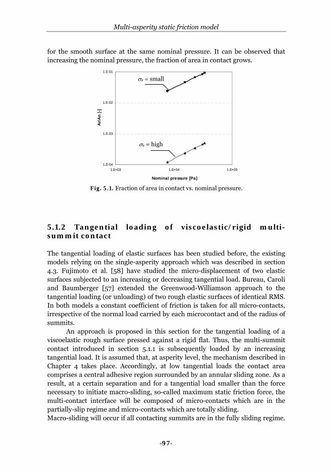
Multi-asperity static friction model
-97-
for the smooth surface at the same nominal pressure. It can be observed that increasing the nominal pressure, the fraction of area in contact grows.
5.1.2 Tangential loading of viscoelastic/rigid multi-summit contact The tangential loading of elastic surfaces has been studied before, the existing models relying on the single-asperity approach which was described in section 4.3. Fujimoto et al. [58] have studied the micro-displacement of two elastic surfaces subjected to an increasing or decreasing tangential load. Bureau, Caroli and Baumberger [57] extended the Greenwood-Williamson approach to the tangential loading (or unloading) of two rough elastic surfaces of identical RMS. In both models a constant coefficient of friction is taken for all micro-contacts, irrespective of the normal load carried by each microcontact and of the radius of summits. An approach is proposed in this section for the tangential loading of a viscoelastic rough surface pressed against a rigid flat. Thus, the multi-summit contact introduced in section 5.1.1 is subsequently loaded by an increasing tangential load. It is assumed that, at asperity level, the mechanism described in Chapter 4 takes place. Accordingly, at low tangential loads the contact area comprises a central adhesive region surrounded by an annular sliding zone. As a result, at a certain separation and for a tangential load smaller than the force necessary to initiate macro-sliding, so-called maximum static friction force, the multi-contact interface will be composed of micro-contacts which are in the partially-slip regime and micro-contacts which are totally sliding. Macro-sliding will occur if all contacting summits are in the fully sliding regime.
1.E-04
1.E-03
1.E-02
1.E-01
1.E+03 1.E+04 1.E+05
Nominal pressure [Pa]
Ar/A
n [-]
Fig. 5.1. Fraction of area in contact vs. nominal pressure.
σs = small
σs = high
Chapter 5
-98-
A condition has been set for an elastic multi-contact interface by Bureau, Caroli and Baumberger [57] which provides a critical summit height above which the micro-contacts are partially sliding. In their approach, a constant local coefficient of friction is considered for all micro-contacts. Using the method presented in [57], a critical summit height is derived for a viscoelastic multi-contact interface. From the single-asperity static friction model (equation 4.44) it follows that:
( ) ( ) ( )⎥⎥
⎦
⎤
⎢⎢
⎣
⎡⎟⎟⎠
⎞⎜⎜⎝
⎛⋅
−−⋅−⋅⋅=3/2
112n
tntv F
Fttμ
νμδδ (5.5)
where δtv is the remote tangential displacement or preliminary displacement and μ is the local coefficient of static friction. Rearranging the factors in equation (5.5) leads to:
( )
( ) ( )
3/2
12
1 ⎟⎟⎠
⎞⎜⎜⎝
⎛⋅
−=−⋅⋅
−n
t
n
tv
FF
tt
μνμδδ
(5.6)
The right-hand side of equation (5.6) is a positive real number for Ft ≤ μ·Fn, thus:
( )
( ) ( )ttn
tv δνμ
δ≤
−⋅ 2 (5.7)
The indentation depth of the summit δn can be replaced by (z - h), as follows from the multi-summit geometry depicted in Figure 3.16. Then, the inequality (5.7) becomes:
( )
( ) htz tv +⋅−
≥μν
δ2
(5.8)
From equation (5.8) it can be inferred that the summits which have the height:
( )
( ) ( ) hF
tsn
tvc +
⋅−≤
μνδ
2 (5.9)
are in the fully sliding regime because they carry a tangential force which is equal to or larger than the maximum static friction force. The micro-contacts of which heights satisfy the relation z ≥ sc are in the partially-slip regime. The assumption of Bureau et al. of a constant local coefficient of friction is removed in this approach. Instead, a local coefficient of friction μ(Fn) which depends on the normal load carried by each micro-contact is used instead. μ(Fn)

Multi-asperity static friction model
-99-
can be obtained from the static friction model presented in Chapter 4. The tangential displacement δtv is the same for all micro-contacts and is equal to the displacement of the mass center of the body, denoted by global tangential displacement, because it is assumed that the rubber is not subjected to bulk strain. The total tangential load carried by the multi-contact interface can be written as: slipstickt FFF += (5.10) where Fstick component is calculated as the sum of all tangential loads carried by the micro-contacts which are not fully sliding. That means that their contact areas are composed of stick and slip regions. Fstick component is given by equation:
( ) ( ) ( ) ( ) ( ) ( ) ( ) ( )∫∞
⎥⎥⎥
⎦
⎤
⎢⎢⎢
⎣
⎡
⎟⎟⎠
⎞⎜⎜⎝
⎛⋅⋅−⋅−
−−⋅⋅⋅−⋅⋅⋅⋅⋅⋅=cs n
tnnstick sd
FhsFshs
tAtF
23
23
21
23
2111
38
σμνδμΘβ
ϕση
(5.11) The Fslip component is taken as the sum of all tangential loads carried by the micro-contacts which are fully sliding and is calculated with equation:
( ) ( ) ( ) ( ) ( )∫ ⋅⋅⋅−⋅⋅⋅⋅⋅⋅=cs
hnnslip sdFshs
tAtF μΘβ
ϕση 2
321
23
138
(5.12)
5.1.3 Static friction of viscoelastic/rigid multi-summit contact Having obtained the tangential load carried by the multi-contact interface, the maximum force required to initiate macro-sliding (or maximum static friction force) can be determined as the sum of all tangential loads causing gross sliding of all micro-contacts. When this condition is obeyed, the partially sliding component Fstick becomes zero and the condition can be written as: 0max == stickslipst FifFF (5.13) The algorithm used in calculation of the maximum static friction force and global coefficient of static friction between surfaces is presented in Figure 5.2. Given the micro-geometry, the nominal area and the material parameters the real

Chapter 5
-100-
contact area and the separation can be calculated. At a certain time instant the normal load carried by the critical asperity can be determined. Then, assuming a tangential displacement the critical height is obtained. For the mean summit radius β the function μ(Fn) can be determined using the single-asperity static friction model. Next, the tangential load carried by each microcontact is calculated. If the partially slip component of the tangential force is not zero the tangential displacement is further increased until all micro-contacts are fully sliding. This maximum tangential displacement corresponding to the occurrence of macro-sliding is taken as the global limiting displacement. At this stage, the maximum static friction force is reached.
Fig. 5.2. Flowchart – calculation of global coefficient of static friction.
microgeometry β, η, σ nominal area An
material and interfacial layer parameters φ(t), hi, g3, η2
time instant t local coefficient of friction μ(Fn)
tangential displ. δtv normal load Fnt
real contact area Ar eqn. (5.3)
separation h eqn. (5.4)
critical height sc eqn. (5.9)
Fstick eqn. (5.11) Fslip eqn. (5.12)
Fst max = Fslip
if Fstick = 0
μsg = Fst max / Fnt
yes
change δt no
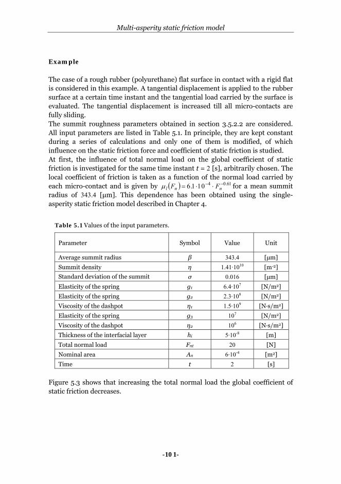
Multi-asperity static friction model
-101-
Example The case of a rough rubber (polyurethane) flat surface in contact with a rigid flat is considered in this example. A tangential displacement is applied to the rubber surface at a certain time instant and the tangential load carried by the surface is evaluated. The tangential displacement is increased till all micro-contacts are fully sliding. The summit roughness parameters obtained in section 3.5.2.2 are considered. All input parameters are listed in Table 5.1. In principle, they are kept constant during a series of calculations and only one of them is modified, of which influence on the static friction force and coefficient of static friction is studied. At first, the influence of total normal load on the global coefficient of static friction is investigated for the same time instant t = 2 [s], arbitrarily chosen. The local coefficient of friction is taken as a function of the normal load carried by each micro-contact and is given by ( ) 610−4− ⋅10⋅16= .. nnl FFμ for a mean summit radius of 343.4 [μm]. This dependence has been obtained using the single-asperity static friction model described in Chapter 4.
Table 5.1 Values of the input parameters.
Parameter Symbol Value Unit
Average summit radius β 343.4 [μm]
Summit density η 1.41·1010 [m-2]
Standard deviation of the summit σ 0.016 [μm]
Elasticity of the spring g1 6.4·107 [N/m2]
Elasticity of the spring g2 2.3·108 [N/m2]
Viscosity of the dashpot η1 1.5·109 [N·s/m2]
Elasticity of the spring g3 107 [N/m2]
Viscosity of the dashpot η2 106 [N·s/m2]
Thickness of the interfacial layer hi 5·10-8 [m]
Total normal load Fnt 20 [N]
Nominal area An 6·10-4 [m2]
Time t 2 [s]
Figure 5.3 shows that increasing the total normal load the global coefficient of static friction decreases.

Chapter 5
-102-
The static friction force versus limiting displacement is plotted in Figure 5.4 for the same normal loads plotted in Figure 5.3. It is observed that both static friction force and limiting displacement increase with normal load. It can be noticed that the static friction force increases much faster than the limiting displacement. A similar trend with respect to the variation of static friction force, preliminary displacement and coefficient of static friction with normal load has been also obtained in the single-asperity case, see section 4.6.3.
0.8
0.9
1
1.1
1.2
1.3
1.4
1.5
0 5 10 15 20
Normal load [N]
Coef
ficie
nt o
f sta
tic fr
ictio
n [-]
Fig. 5.3. Variation of the coefficient of static friction with normal load.
Fig. 5.4. Static friction force (Fs) vs. limiting displacement (δl) for different normal loads.
0
2
4
6
8
10
12
14
16
18
20
2.08E-08 2.13E-08 2.18E-08 2.23E-08 2.28E-08 2.33E-08 2.38E-08 2.43E-08 2.48E-08
Limiting displacement [m]
Stat
ic fr
ictio
n fo
rce
[N]
1
5
10
15
20
Fnt[N]
Ff
δt δl
Fn ↑
Fn ↑
Fs

Multi-asperity static friction model
-103-
Secondly, the influence of surface roughness on the coefficient of static friction has been investigated. The average roughness Ra has been modified by varying the mean summit radius β and the standard deviation of the summit heights σ, and keeping the summit density η and the product of these three parameters constant. By decreasing the average summit radius and increasing the standard deviation of the summit heights, smoother surfaces can be simulated, that means smaller Ra. It is worth mentioning that the local coefficient of static friction depends also on the radius of the summit (see Chapter 4). Therefore, the dependence of the local coefficient of static friction on normal load for several summit radii which corresponds to several Ra has been determined. These functions are presented in Table 5.2. The rest of the input parameters are the same as those given in Table 5.1.
Table 5.2. μl (Fn) for different summit radii.
Average summit
radius, β [μm] μl (Fn)
343 μl(Fn)= 6.1·10-4 ·Fn-0.61
90 μl(Fn)= 4.7·10-4 ·Fn-0.58
50 μl(Fn)= 4.4·10-4 ·Fn-0.57
10 μl(Fn)= 5.4·10-4 ·Fn-0.47
Figure 5.5 indicates that rougher surfaces, i.e. larger Ra, result in smaller coefficients of static friction, while smoother surfaces determine higher coefficients of static friction. In particular, very smooth surfaces Ra < 0.1 [μm] will result in high coefficients of static friction.
0
0.1
0.2
0.3
0.4
0.5
0.6
0.7
0.8
0.9
1
1.3E-08 6.3E-08 1.1E-07 1.6E-07 2.1E-07 2.6E-07 3.1E-07 3.6E-07 4.1E-07
Ra [m]
Coef
ficie
nt o
f sta
tic fr
ictio
n [-]
Fig. 5.5. Variation of the coefficient of static friction with the average roughness Ra.
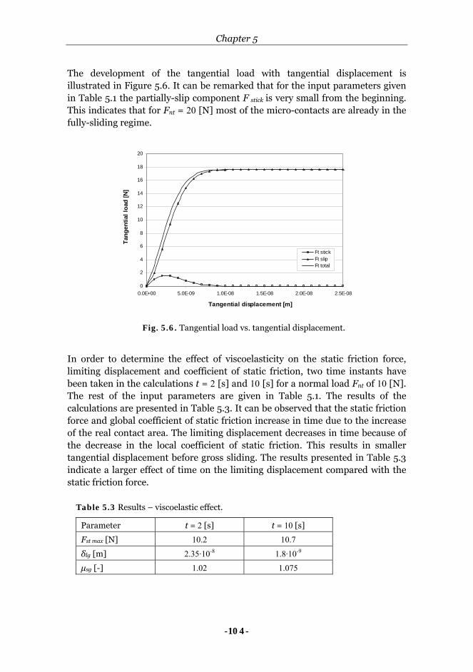
Chapter 5
-104-
The development of the tangential load with tangential displacement is illustrated in Figure 5.6. It can be remarked that for the input parameters given in Table 5.1 the partially-slip component F stick is very small from the beginning. This indicates that for Fnt = 20 [N] most of the micro-contacts are already in the fully-sliding regime.
In order to determine the effect of viscoelasticity on the static friction force, limiting displacement and coefficient of static friction, two time instants have been taken in the calculations t = 2 [s] and 10 [s] for a normal load Fnt of 10 [N]. The rest of the input parameters are given in Table 5.1. The results of the calculations are presented in Table 5.3. It can be observed that the static friction force and global coefficient of static friction increase in time due to the increase of the real contact area. The limiting displacement decreases in time because of the decrease in the local coefficient of static friction. This results in smaller tangential displacement before gross sliding. The results presented in Table 5.3 indicate a larger effect of time on the limiting displacement compared with the static friction force.
Table 5.3 Results – viscoelastic effect.
Parameter t = 2 [s] t = 10 [s]
Fst max [N] 10.2 10.7
δlg [m] 2.35·10-8 1.8·10-9
μsg [-] 1.02 1.075
0
2
4
6
8
10
12
14
16
18
20
0.0E+00 5.0E-09 1.0E-08 1.5E-08 2.0E-08 2.5E-08
Tangential displacement [m]
Tang
entia
l loa
d [N
]
Ft stickFt slipFt total
Fig. 5.6. Tangential load vs. tangential displacement.

Multi-asperity static friction model
-105-
5.2 Viscoelastic/rigid multi-asperity contact (type III)
5.2.1 Viscoelastic/rigid multi-asperity contact model Equivalent asperities versus summits The multi-asperity contact or type III contact has been previously introduced in section 3.5.4. In this chapter, the multi-asperity contact model characterized by large microcontacts will be called deterministic model. According to this approach, the surface roughness can be modeled as composed of many asperities which have different radii and different heights. Moreover, the multi-asperity contact model takes into account the merging of adjacent asperities into “equivalent asperities” at higher normal loads (or smaller separations between surfaces) as described by Masen and de Rooij [59]. The merging of asperities at smaller separations is depicted in Figure 5.7. The equations for the radii and height of the equivalent asperity have been given in Appendix A, see equations (A1) to (A3).
When comparing the statistical case with the deterministic case, a first observation is that the number of contacting equivalent asperities is usually much smaller than the number of contacting summits at the same normal load. This is illustrated in Figure 5.8 and Figure 5.9 where the locations of the summits and equivalent asperities are plotted at a normal load of 10-2 [N] (pn = 6.7·104Pa). The input parameters used in the calculations are given in Table 5.4.
Fig. 5.7. Merging of adjacent asperities into equivalent asperities at smaller separations between surfaces, adapted from [59].
h1
h2 < h1
equivalent asperity at
separation h2
asperity 2 at separation h1 asperity 1
at separation h1
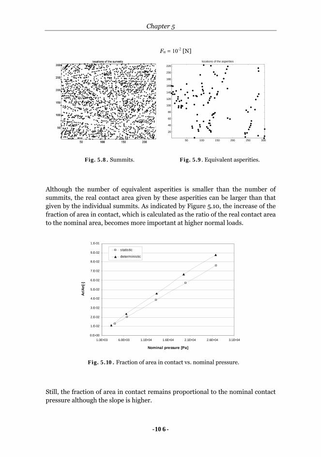
Chapter 5
-106-
Although the number of equivalent asperities is smaller than the number of summits, the real contact area given by these asperities can be larger than that given by the individual summits. As indicated by Figure 5.10, the increase of the fraction of area in contact, which is calculated as the ratio of the real contact area to the nominal area, becomes more important at higher normal loads.
Still, the fraction of area in contact remains proportional to the nominal contact pressure although the slope is higher.
Fig. 5.10. Fraction of area in contact vs. nominal pressure.
0.E+00
1.E-02
2.E-02
3.E-02
4.E-02
5.E-02
6.E-02
7.E-02
8.E-02
9.E-02
1.E-01
1.0E+03 6.0E+03 1.1E+04 1.6E+04 2.1E+04 2.6E+04 3.1E+04
Nominal pressure [Pa]
Ar/A
n[-]
statistic
deterministic
Fn = 10-2 [N]
Fig. 5.9. Equivalent asperities. Fig. 5.8. Summits.
50 100 150 200 250 300
20
40
60
80
100
120
140
160
180
200
220locations of the asperities
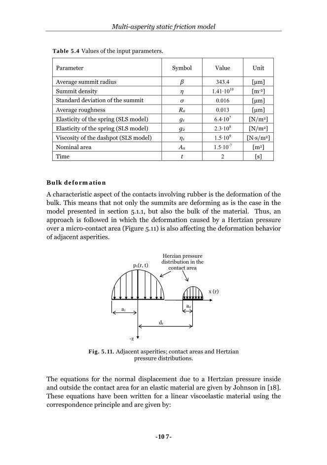
Multi-asperity static friction model
-107-
Table 5.4 Values of the input parameters.
Parameter Symbol Value Unit
Average summit radius β 343.4 [μm]
Summit density η 1.41·1010 [m-2]
Standard deviation of the summit σ 0.016 [μm]
Average roughness Ra 0.013 [μm]
Elasticity of the spring (SLS model) g1 6.4·107 [N/m2]
Elasticity of the spring (SLS model) g2 2.3·108 [N/m2]
Viscosity of the dashpot (SLS model) η1 1.5·109 [N·s/m2]
Nominal area An 1.5·10-7 [m2]
Time t 2 [s]
Bulk deformation
A characteristic aspect of the contacts involving rubber is the deformation of the bulk. This means that not only the summits are deforming as is the case in the model presented in section 5.1.1, but also the bulk of the material. Thus, an approach is followed in which the deformation caused by a Hertzian pressure over a micro-contact area (Figure 5.11) is also affecting the deformation behavior of adjacent asperities.
The equations for the normal displacement due to a Hertzian pressure inside and outside the contact area for an elastic material are given by Johnson in [18]. These equations have been written for a linear viscoelastic material using the correspondence principle and are given by:
Fig. 5.11. Adjacent asperities; contact areas and Hertzian pressure distributions.
-z
Herzian pressure distribution in the
contact area p1(r, t)
x (r)
a1
dr
a2
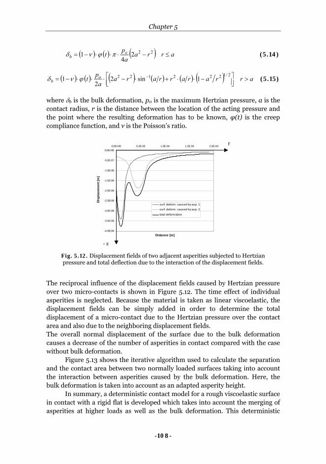
Chapter 5
-108-
( ) ( ) ( ) arraa
pt ob ≤−⋅⋅⋅−= 222
41 πϕνδ (5.14)
( ) ( ) ( ) ( ) ( ) ( ) arrararraraa
pt ob >⎥⎦
⎤⎢⎣⎡ −⋅⋅+⋅−⋅⋅⋅−= − 2/1222122 1sin2
21 ϕνδ (5.15)
where δb is the bulk deformation, p0 is the maximum Hertzian pressure, a is the contact radius, r is the distance between the location of the acting pressure and the point where the resulting deformation has to be known, φ(t) is the creep compliance function, and ν is the Poisson’s ratio.
The reciprocal influence of the displacement fields caused by Hertzian pressure over two micro-contacts is shown in Figure 5.12. The time effect of individual asperities is neglected. Because the material is taken as linear viscoelastic, the displacement fields can be simply added in order to determine the total displacement of a micro-contact due to the Hertzian pressure over the contact area and also due to the neighboring displacement fields. The overall normal displacement of the surface due to the bulk deformation causes a decrease of the number of asperities in contact compared with the case without bulk deformation. Figure 5.13 shows the iterative algorithm used to calculate the separation and the contact area between two normally loaded surfaces taking into account the interaction between asperities caused by the bulk deformation. Here, the bulk deformation is taken into account as an adapted asperity height. In summary, a deterministic contact model for a rough viscoelastic surface in contact with a rigid flat is developed which takes into account the merging of asperities at higher loads as well as the bulk deformation. This deterministic
Fig. 5.12. Displacement fields of two adjacent asperities subjected to Hertzian pressure and total deflection due to the interaction of the displacement fields.
r
- z
-4.0E-06
-3.5E-06
-3.0E-06
-2.5E-06
-2.0E-06
-1.5E-06
-1.0E-06
-5.0E-07
0.0E+000.0E+00 5.0E-05 1.0E-04 1.5E-04 2.0E-04
Distance [m]
Disp
lace
men
t [m
]
surf. deform. caused by asp. 1
surf. deform. caused by asp. 2
total deformation
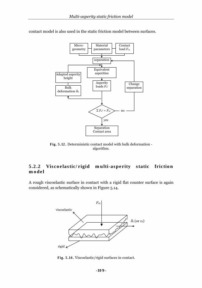
Multi-asperity static friction model
-109-
contact model is also used in the static friction model between surfaces.
5.2.2 Viscoelastic/rigid multi-asperity static friction model A rough viscoelastic surface in contact with a rigid flat counter surface is again considered, as schematically shown in Figure 5.14.
Micro-geometry
Material parameters
Contact load Fnt
Bulk deformation δb
Adapted asperity height
separation
Equivalent asperities
Asperity loads Fni
Change separation
Σ Fni = Fnt
Separation Contact area
yes
no
Fig. 5.12. Deterministic contact model with bulk deformation -algorithm.
Fnt
δt (or vt)
viscoelastic
rigid
Fig. 5.14. Viscoelastic/rigid surfaces in contact.

Chapter 5
-110-
By applying a normal load Fnt, a number of micro-contacts are created. Subsequent application of a tangential displacement δt will cause slipping of a part of the micro-contacts while the rest of them will still be in contact with the rigid flat. At a certain tangential displacement denoted as limiting displacement δlg, all the micro-contacts are broken, leading to the full sliding of one surface with respect to the other. This is the moment corresponding to the maximum static friction force Fst max. Then, the static friction force between surfaces is calculated as the sum of all static friction forces of the individual asperities in contact. These individual static friction forces can be obtained from the single-asperity static friction model described in Chapter 4.
locations of micro-contacts
micro-geometry radius, height of
asperities
normal load carried by each micro-contact
time instant t tangential displacement
δt(t)
static friction time tsi of each micro-contact
tangential load Fti carried by each micro-contact
t ≥ ts Fti = Fslip eqn. (5.16)
t < ts Fti = Fstick eqn. (5.17)
material properties φ(t) interfacial layer properties
hi, g3, η2
nominal area An normal load Fnt
if all Fsticki = 0
increase t
no
yes
Fst max = Σ Fslip
μgs = Fst max/Fn
Fig. 5.15. Multi-asperity static friction model – algorithm.
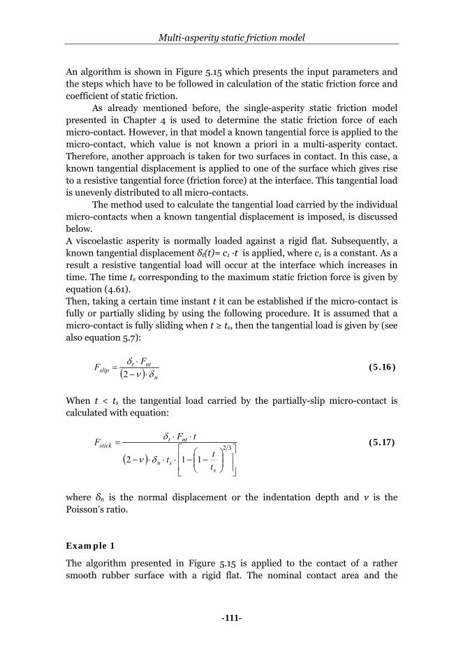
Multi-asperity static friction model
-111-
An algorithm is shown in Figure 5.15 which presents the input parameters and the steps which have to be followed in calculation of the static friction force and coefficient of static friction. As already mentioned before, the single-asperity static friction model presented in Chapter 4 is used to determine the static friction force of each micro-contact. However, in that model a known tangential force is applied to the micro-contact, which value is not known a priori in a multi-asperity contact. Therefore, another approach is taken for two surfaces in contact. In this case, a known tangential displacement is applied to one of the surface which gives rise to a resistive tangential force (friction force) at the interface. This tangential load is unevenly distributed to all micro-contacts.
The method used to calculate the tangential load carried by the individual micro-contacts when a known tangential displacement is imposed, is discussed below. A viscoelastic asperity is normally loaded against a rigid flat. Subsequently, a known tangential displacement δt(t)= c1 ·t is applied, where c1 is a constant. As a result a resistive tangential load will occur at the interface which increases in time. The time ts corresponding to the maximum static friction force is given by equation (4.61). Then, taking a certain time instant t it can be established if the micro-contact is fully or partially sliding by using the following procedure. It is assumed that a micro-contact is fully sliding when t ≥ ts, then the tangential load is given by (see also equation 5.7):
( ) n
nttslip
FFδν
δ⋅−
⋅=
2 (5.16)
When t < ts the tangential load carried by the partially-slip micro-contact is calculated with equation:
( )⎥⎥
⎦
⎤
⎢⎢
⎣
⎡⎟⎟⎠
⎞⎜⎜⎝
⎛−−⋅⋅⋅−
⋅⋅=
32
112s
sn
nttstick
ttt
tFF
δν
δ (5.17)
where δn is the normal displacement or the indentation depth and ν is the Poisson’s ratio. Example 1
The algorithm presented in Figure 5.15 is applied to the contact of a rather smooth rubber surface with a rigid flat. The nominal contact area and the
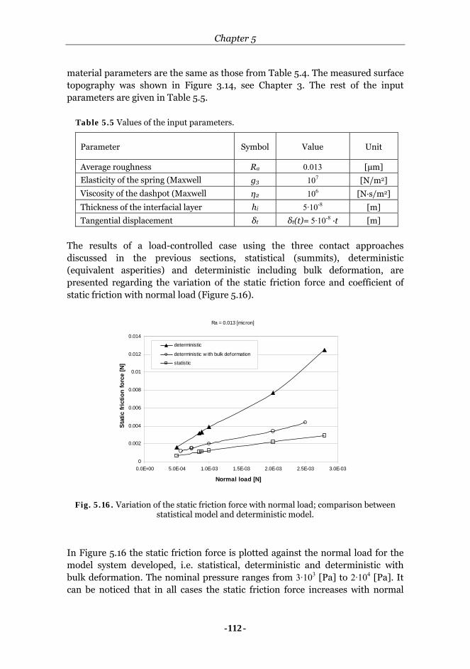
Chapter 5
-112-
material parameters are the same as those from Table 5.4. The measured surface topography was shown in Figure 3.14, see Chapter 3. The rest of the input parameters are given in Table 5.5.
Table 5.5 Values of the input parameters.
Parameter Symbol Value Unit
Average roughness Ra 0.013 [μm]
Elasticity of the spring (Maxwell g3 107 [N/m2]
Viscosity of the dashpot (Maxwell η2 106 [N·s/m2]
Thickness of the interfacial layer hi 5·10-8 [m]
Tangential displacement δt δt(t)= 5·10-8 ·t [m]
The results of a load-controlled case using the three contact approaches discussed in the previous sections, statistical (summits), deterministic (equivalent asperities) and deterministic including bulk deformation, are presented regarding the variation of the static friction force and coefficient of static friction with normal load (Figure 5.16).
In Figure 5.16 the static friction force is plotted against the normal load for the model system developed, i.e. statistical, deterministic and deterministic with bulk deformation. The nominal pressure ranges from 3·103 [Pa] to 2·104 [Pa]. It can be noticed that in all cases the static friction force increases with normal
Ra = 0.013 [micron]
0
0.002
0.004
0.006
0.008
0.01
0.012
0.014
0.0E+00 5.0E-04 1.0E-03 1.5E-03 2.0E-03 2.5E-03 3.0E-03
Normal load [N]
Stat
ic fr
ictio
n fo
rce
[N]
deterministic
deterministic w ith bulk deformation
statistic
Fig. 5.16. Variation of the static friction force with normal load; comparison between statistical model and deterministic model.
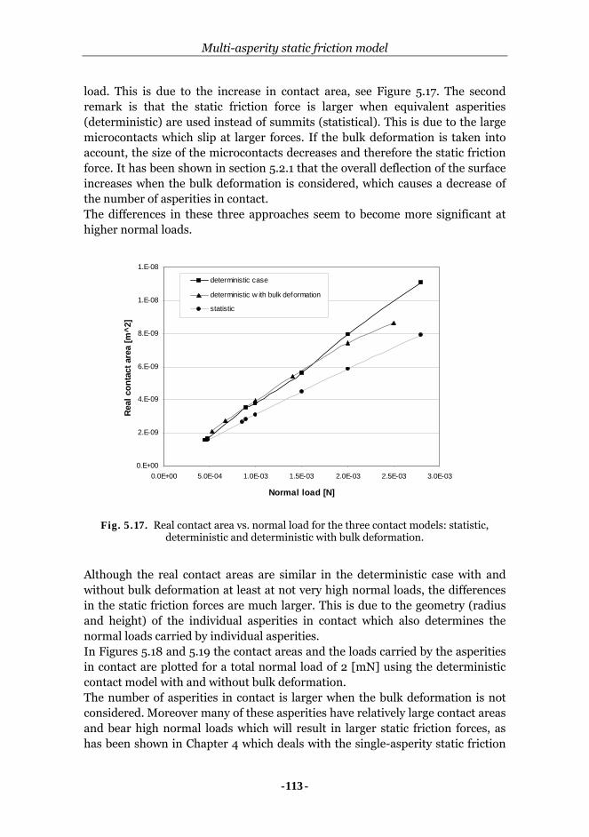
Multi-asperity static friction model
-113-
load. This is due to the increase in contact area, see Figure 5.17. The second remark is that the static friction force is larger when equivalent asperities (deterministic) are used instead of summits (statistical). This is due to the large microcontacts which slip at larger forces. If the bulk deformation is taken into account, the size of the microcontacts decreases and therefore the static friction force. It has been shown in section 5.2.1 that the overall deflection of the surface increases when the bulk deformation is considered, which causes a decrease of the number of asperities in contact. The differences in these three approaches seem to become more significant at higher normal loads.
Although the real contact areas are similar in the deterministic case with and without bulk deformation at least at not very high normal loads, the differences in the static friction forces are much larger. This is due to the geometry (radius and height) of the individual asperities in contact which also determines the normal loads carried by individual asperities. In Figures 5.18 and 5.19 the contact areas and the loads carried by the asperities in contact are plotted for a total normal load of 2 [mN] using the deterministic contact model with and without bulk deformation. The number of asperities in contact is larger when the bulk deformation is not considered. Moreover many of these asperities have relatively large contact areas and bear high normal loads which will result in larger static friction forces, as has been shown in Chapter 4 which deals with the single-asperity static friction
0.E+00
2.E-09
4.E-09
6.E-09
8.E-09
1.E-08
1.E-08
0.0E+00 5.0E-04 1.0E-03 1.5E-03 2.0E-03 2.5E-03 3.0E-03
Normal load [N]
Real
con
tact
are
a [m
^2]
deterministic case
deterministic w ith bulk deformation
statistic
Fig. 5.17. Real contact area vs. normal load for the three contact models: statistic, deterministic and deterministic with bulk deformation.
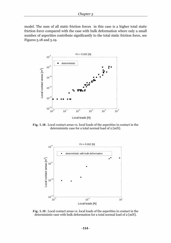
Chapter 5
-114-
model. The sum of all static friction forces in this case is a higher total static friction force compared with the case with bulk deformation where only a small number of asperities contribute significantly to the total static friction force, see Figures 5.18 and 5.19.
10-5 10-4 10-310-11
10-10
10-9
10-8
Local loads [N]
Loca
l con
tact
are
as [m
2 ]
Fn = 0.002 [N]
deterministic with bulk deformation
Fig. 5.19. Local contact areas vs. local loads of the asperities in contact in the deterministic case with bulk deformation for a total normal load of 2 [mN].
10-8 10-7 10-6 10-5 10-4 10-310-13
10-12
10-11
10-10
10-9
10-8
Local loads [N]
Loca
l con
tact
are
as [m
2 ]
Fn = 0.002 [N]
deterministic
Fig. 5.18. Local contact areas vs. local loads of the asperities in contact in the deterministic case for a total normal load of 2 [mN].

Multi-asperity static friction model
-115-
In the statistical case the number of summits in contact is quite large compared to the number of asperities in the other two models. However, most of them carry very low loads which will result in smaller static friction forces.
Unlike the static friction force, the variation of the coefficient of static friction with normal load shows different trends for all three approaches, see Figure 5.20. In the statistical case, the coefficient of static friction decreases by increasing normal load. An increase of the coefficient of static friction is observed in the deterministic case. Taking into account the bulk deformation in the deterministic model, the coefficient of friction initially decreases similarly to the statistic case, then slightly increases at higher loads. Although in all cases (see Figure 5.16) the static friction force increases with normal load, the coefficient of static friction may slightly increase or decrease. This can be explained by the rate of increase of the static friction force which can be larger/smaller than that of the normal load. Example 2
A second example is considered in which the same nominal area is taken in the calculations with a different surface topography having an average roughness Ra = 0.068 [μm]. The rest of the input parameters are the same as in example 1. It can be observed from Figure 5.21 that, similarly to the results plotted in
Ra = 0.013 [micron]
0
0.5
1
1.5
2
2.5
3
3.5
4
4.5
5
0.0E+00 5.0E-04 1.0E-03 1.5E-03 2.0E-03 2.5E-03 3.0E-03
Normal load [N]
Coef
ficie
nt o
f sta
tic fr
ictio
n [-]
deterministicdeterministic w ith bulk deformationstatistic
Fig. 5.20. Variation of the coefficient of static friction with normal load; comparison between statistical model and deterministic model.
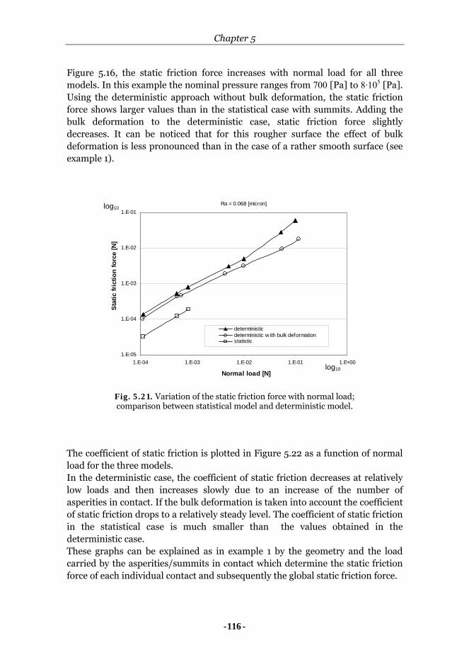
Chapter 5
-116-
Figure 5.16, the static friction force increases with normal load for all three models. In this example the nominal pressure ranges from 700 [Pa] to 8·105 [Pa]. Using the deterministic approach without bulk deformation, the static friction force shows larger values than in the statistical case with summits. Adding the bulk deformation to the deterministic case, static friction force slightly decreases. It can be noticed that for this rougher surface the effect of bulk deformation is less pronounced than in the case of a rather smooth surface (see example 1).
The coefficient of static friction is plotted in Figure 5.22 as a function of normal load for the three models. In the deterministic case, the coefficient of static friction decreases at relatively low loads and then increases slowly due to an increase of the number of asperities in contact. If the bulk deformation is taken into account the coefficient of static friction drops to a relatively steady level. The coefficient of static friction in the statistical case is much smaller than the values obtained in the deterministic case. These graphs can be explained as in example 1 by the geometry and the load carried by the asperities/summits in contact which determine the static friction force of each individual contact and subsequently the global static friction force.
Ra = 0.068 [micron]
1.E-05
1.E-04
1.E-03
1.E-02
1.E-01
1.E-04 1.E-03 1.E-02 1.E-01 1.E+00
Normal load [N]
Stat
ic fr
ictio
n fo
rce
[N]
deterministicdeterministic w ith bulk deformationstatistic
log10
log10
Fig. 5.21. Variation of the static friction force with normal load; comparison between statistical model and deterministic model.
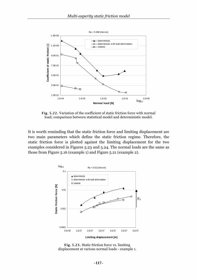
Multi-asperity static friction model
-117-
It is worth reminding that the static friction force and limiting displacement are two main parameters which define the static friction regime. Therefore, the static friction force is plotted against the limiting displacement for the two examples considered in Figures 5.23 and 5.24. The normal loads are the same as those from Figure 5.16 (example 1) and Figure 5.21 (example 2).
Ra = 0.068 [micron]
1.0E-01
3.0E-01
5.0E-01
7.0E-01
9.0E-01
1.1E+00
1.3E+00
1.E-04 1.E-03 1.E-02 1.E-01 1.E+00
Normal load [N]
Coe
ffici
ent o
f sta
tic fr
ictio
n [-]
deterministic deterministic w ith bulk deformationstatistic
log10
Fig. 5.22. Variation of the coefficient of static friction force with normal load; comparison between statistical model and deterministic model.
Ra = 0.013 [micron]
0.0001
0.001
0.01
0.1
0.E+00 1.E-07 2.E-07 3.E-07 4.E-07 5.E-07 6.E-07
Limiting displacement [m]
Stat
ic fr
ictio
n fo
rce
[N]
deterministicdeterministic w ith bulk deformationstatistic
Fig. 5.23. Static friction force vs. limiting displacement at various normal loads - example 1.
Fn
log10
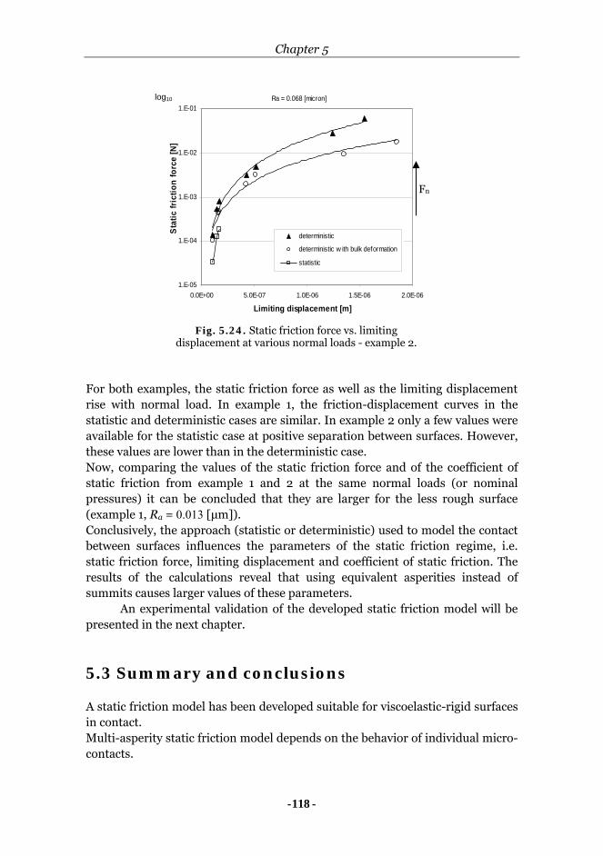
Chapter 5
-118-
For both examples, the static friction force as well as the limiting displacement rise with normal load. In example 1, the friction-displacement curves in the statistic and deterministic cases are similar. In example 2 only a few values were available for the statistic case at positive separation between surfaces. However, these values are lower than in the deterministic case. Now, comparing the values of the static friction force and of the coefficient of static friction from example 1 and 2 at the same normal loads (or nominal pressures) it can be concluded that they are larger for the less rough surface (example 1, Ra = 0.013 [μm]). Conclusively, the approach (statistic or deterministic) used to model the contact between surfaces influences the parameters of the static friction regime, i.e. static friction force, limiting displacement and coefficient of static friction. The results of the calculations reveal that using equivalent asperities instead of summits causes larger values of these parameters. An experimental validation of the developed static friction model will be presented in the next chapter.
5.3 Summary and conclusions A static friction model has been developed suitable for viscoelastic-rigid surfaces in contact. Multi-asperity static friction model depends on the behavior of individual micro-contacts.
Ra = 0.068 [micron]
1.E-05
1.E-04
1.E-03
1.E-02
1.E-01
0.0E+00 5.0E-07 1.0E-06 1.5E-06 2.0E-06
Limiting displacement [m]
Sta
tic fr
ictio
n fo
rce
[N]
deterministic
deterministic w ith bulk deformation
statistic
log10
Fn
Fig. 5.24. Static friction force vs. limiting displacement at various normal loads - example 2.
Multi-asperity static friction model
-119-
Three approaches have been used to model the contact between a viscoelastic surface and rigid flat. The statistical or multi-summit approach offers a simplified solution, based on summits which do not interact with each other. The multi-asperity or deterministic model is a more realistic approach which takes into account the merging of asperities at larger loads and also the bulk deformation. Using a deterministic approach that means equivalent asperities instead of summits, the static friction force as well as the coefficient of static friction are larger compared to the statistical approach. Static friction force and limiting displacement are typically larger when the deterministic approach is used. The geometry of asperities and the normal load carried by the asperities in contact determine the individual static friction forces which compose the global static friction force. In the deterministic case the number of asperities which have a significant contribution to the total friction force due to their large contact areas and high normal loads is larger than in the statistical case and also in the case with bulk deformation. The results presented in this chapter show that rough surfaces result in smaller coefficients of static friction.

Chapter 5
-120-

-121-
Chapter 6 Experimental results and validation of the
static friction models
Introduction
A multi-asperity static friction model has been presented in Chapter 5 which is based on the single-asperity model introduced in Chapter 4. In this chapter, these theoretical models are experimentally validated. The materials used in the experiments have been characterized in Chapter 3 and 4. Single-asperity friction measurements have been carried out on a nano-tribometer using a ball-on-flat configuration. The influence of several parameters such as normal load, radius of the ball and elasticity modulus (creep compliance) upon static friction was examined. The experimental results correlate well with the calculations. Then, the multi-asperity static friction model is validated. The coefficient of static friction was investigated at several normal loads. The experimental results resemble the theoretical predictions.
6.1 Single-asperity static friction measurements The single-asperity contact can be simply described by a sphere in contact with a flat. This approach will be used to investigate experimentally static friction between a rubber flat and a rigid asperity. It is important to mention that in the single-asperity static friction model a rubber asperity has been loaded against a rigid flat in order to study the adhesive component of friction. In this way the ploughing component of friction was avoided. In the experiments, the opposite case, i.e. rigid ball against rubber flat, has been used. However, by keeping the normal indentation (or strain) small, the ploughing component can be neglected. In this way, rubber plates similar to those used in industrial applications (rubber pad forming), of which properties were already determined, can be used. The experimental investigation has been carried out on a special tribometer which is described in the next section.
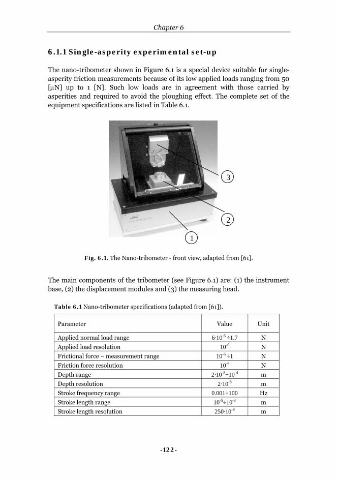
Chapter 6
-122-
6.1.1 Single-asperity experimental set-up The nano-tribometer shown in Figure 6.1 is a special device suitable for single-asperity friction measurements because of its low applied loads ranging from 50 [μN] up to 1 [N]. Such low loads are in agreement with those carried by asperities and required to avoid the ploughing effect. The complete set of the equipment specifications are listed in Table 6.1.
The main components of the tribometer (see Figure 6.1) are: (1) the instrument base, (2) the displacement modules and (3) the measuring head.
Table 6.1 Nano-tribometer specifications (adapted from [61]).
Parameter Value Unit
Applied normal load range 6·10-5 ÷1.7 N
Applied load resolution 10-6 N
Frictional force – measurement range 10-5 ÷1 N
Friction force resolution 10-6 N
Depth range 2·10-8÷10-4 m
Depth resolution 2·10-8 m
Stroke frequency range 0.001÷100 Hz
Stroke length range 10-5÷10-3 m
Stroke length resolution 250·10-8 m
2
1
3
Fig. 6.1. The Nano-tribometer - front view, adapted from [61].

Experimental results and validation of the static friction models
-123-
The instrument base (1) contains two stepper motors for x and y directions and the electronic units. Two displacement modules, linear reciprocating and pin-on-disc, are available for static and dynamic friction measurements. The measuring head (Figure 6.2) is composed of a cantilever (4) with two associated optical sensors for the measurement of normal (5) and lateral (6) deflections and the head actuators (7).
The friction tests were performed in the linear reciprocating mode which is appropriate for static friction measurements. As mentioned before, the single-asperity geometry has been reproduced by a steel ball in contact with polyurethane flat. Method In this thesis the linear reciprocating module is used for studying the friction force in relation to sliding distance or time. A simplified sketch is depicted in Figure 6.3. The ball is glued on a stiff lever, which is part of a frictionless force transducer consisting of elastic springs and optical displacement sensors. The counter sample is attached to a holder which is fixed in the displacement module and is displaced in x-direction by the stepper motor. The normal load is applied through the ball. The friction force is determined during the test by measuring the deflection of the elastic arm.
Fig. 6.2. Details of the measurement head, adapted from [61].
6 5 4 7
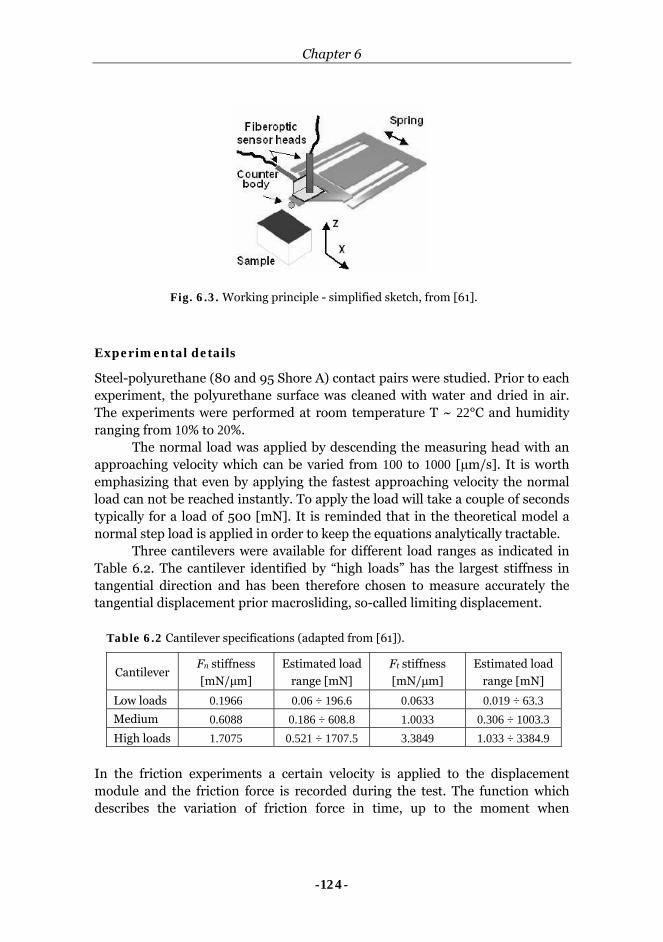
Chapter 6
-124-
Experimental details
Steel-polyurethane (80 and 95 Shore A) contact pairs were studied. Prior to each experiment, the polyurethane surface was cleaned with water and dried in air. The experiments were performed at room temperature T ~ 22°C and humidity ranging from 10% to 20%. The normal load was applied by descending the measuring head with an approaching velocity which can be varied from 100 to 1000 [µm/s]. It is worth emphasizing that even by applying the fastest approaching velocity the normal load can not be reached instantly. To apply the load will take a couple of seconds typically for a load of 500 [mN]. It is reminded that in the theoretical model a normal step load is applied in order to keep the equations analytically tractable. Three cantilevers were available for different load ranges as indicated in Table 6.2. The cantilever identified by “high loads” has the largest stiffness in tangential direction and has been therefore chosen to measure accurately the tangential displacement prior macrosliding, so-called limiting displacement.
Table 6.2 Cantilever specifications (adapted from [61]).
Cantilever Fn stiffness
[mN/μm]
Estimated load
range [mN]
Ft stiffness
[mN/μm]
Estimated load
range [mN]
Low loads 0.1966 0.06 ÷ 196.6 0.0633 0.019 ÷ 63.3 Medium 0.6088 0.186 ÷ 608.8 1.0033 0.306 ÷ 1003.3 High loads 1.7075 0.521 ÷ 1707.5 3.3849 1.033 ÷ 3384.9
In the friction experiments a certain velocity is applied to the displacement module and the friction force is recorded during the test. The function which describes the variation of friction force in time, up to the moment when
Fig. 6.3. Working principle - simplified sketch, from [61].
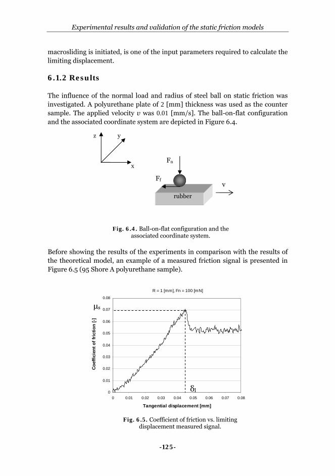
Experimental results and validation of the static friction models
-125-
macrosliding is initiated, is one of the input parameters required to calculate the limiting displacement. 6.1.2 Results The influence of the normal load and radius of steel ball on static friction was investigated. A polyurethane plate of 2 [mm] thickness was used as the counter sample. The applied velocity v was 0.01 [mm/s]. The ball-on-flat configuration and the associated coordinate system are depicted in Figure 6.4.
Before showing the results of the experiments in comparison with the results of the theoretical model, an example of a measured friction signal is presented in Figure 6.5 (95 Shore A polyurethane sample).
v
Fn
Ff
rubber
x
z y
Fig. 6.4. Ball-on-flat configuration and the associated coordinate system.
Fig. 6.5. Coefficient of friction vs. limiting displacement measured signal.
R = 1 [mm], Fn = 100 [mN]
0
0.01
0.02
0.03
0.04
0.05
0.06
0.07
0.08
0 0.01 0.02 0.03 0.04 0.05 0.06 0.07 0.08
Tangential displacement [mm]
Coe
ffici
ent o
f fri
ctio
n [-]
μs
δl
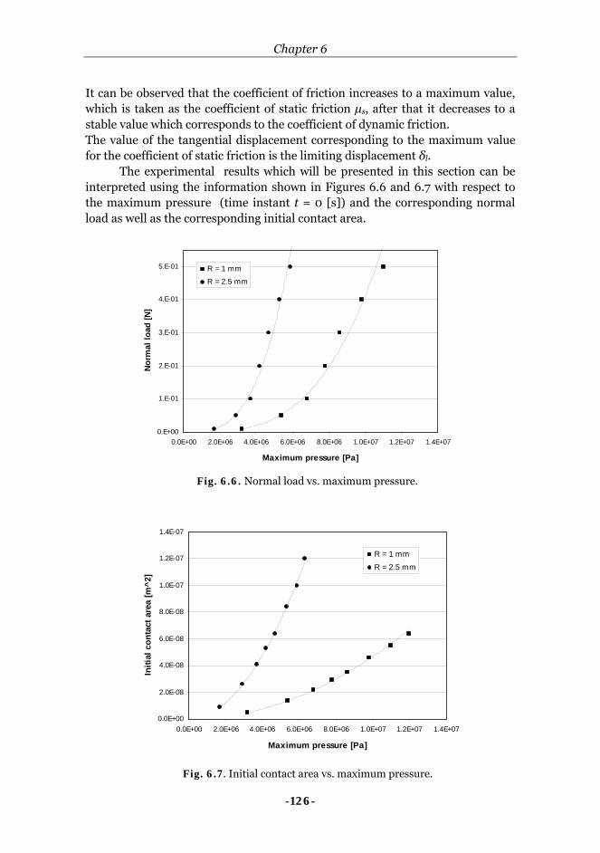
Chapter 6
-126-
It can be observed that the coefficient of friction increases to a maximum value, which is taken as the coefficient of static friction μs, after that it decreases to a stable value which corresponds to the coefficient of dynamic friction. The value of the tangential displacement corresponding to the maximum value for the coefficient of static friction is the limiting displacement δl. The experimental results which will be presented in this section can be interpreted using the information shown in Figures 6.6 and 6.7 with respect to the maximum pressure (time instant t = 0 [s]) and the corresponding normal load as well as the corresponding initial contact area.
Fig. 6.6. Normal load vs. maximum pressure.
0.E+00
1.E-01
2.E-01
3.E-01
4.E-01
5.E-01
0.0E+00 2.0E+06 4.0E+06 6.0E+06 8.0E+06 1.0E+07 1.2E+07 1.4E+07
Maximum pressure [Pa]
Nor
mal
load
[N]
R = 1 mm
R = 2.5 mm
Fig. 6.7. Initial contact area vs. maximum pressure.
0.0E+00
2.0E-08
4.0E-08
6.0E-08
8.0E-08
1.0E-07
1.2E-07
1.4E-07
0.0E+00 2.0E+06 4.0E+06 6.0E+06 8.0E+06 1.0E+07 1.2E+07 1.4E+07
Maximum pressure [Pa]
Initi
al c
onta
ct a
rea
[m^2
]
R = 1 mmR = 2.5 mm
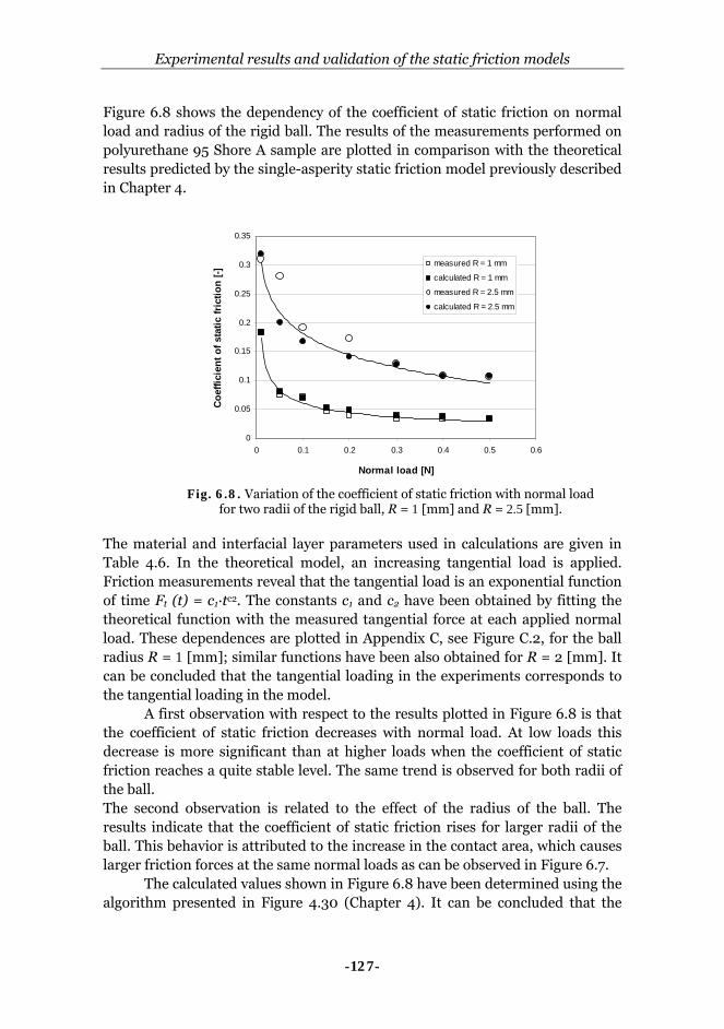
Experimental results and validation of the static friction models
-127-
Figure 6.8 shows the dependency of the coefficient of static friction on normal load and radius of the rigid ball. The results of the measurements performed on polyurethane 95 Shore A sample are plotted in comparison with the theoretical results predicted by the single-asperity static friction model previously described in Chapter 4.
The material and interfacial layer parameters used in calculations are given in Table 4.6. In the theoretical model, an increasing tangential load is applied. Friction measurements reveal that the tangential load is an exponential function of time Ft (t) = c1·tc2. The constants c1 and c2 have been obtained by fitting the theoretical function with the measured tangential force at each applied normal load. These dependences are plotted in Appendix C, see Figure C.2, for the ball radius R = 1 [mm]; similar functions have been also obtained for R = 2 [mm]. It can be concluded that the tangential loading in the experiments corresponds to the tangential loading in the model. A first observation with respect to the results plotted in Figure 6.8 is that the coefficient of static friction decreases with normal load. At low loads this decrease is more significant than at higher loads when the coefficient of static friction reaches a quite stable level. The same trend is observed for both radii of the ball. The second observation is related to the effect of the radius of the ball. The results indicate that the coefficient of static friction rises for larger radii of the ball. This behavior is attributed to the increase in the contact area, which causes larger friction forces at the same normal loads as can be observed in Figure 6.7. The calculated values shown in Figure 6.8 have been determined using the algorithm presented in Figure 4.30 (Chapter 4). It can be concluded that the
Fig. 6.8. Variation of the coefficient of static friction with normal load for two radii of the rigid ball, R = 1 [mm] and R = 2.5 [mm].
0
0.05
0.1
0.15
0.2
0.25
0.3
0.35
0 0.1 0.2 0.3 0.4 0.5 0.6
Normal load [N]
Coe
ffici
ent o
f sta
tic fr
ictio
n [-]
measured R = 1 mm
calculated R = 1 mm
measured R = 2.5 mm
calculated R = 2.5 mm
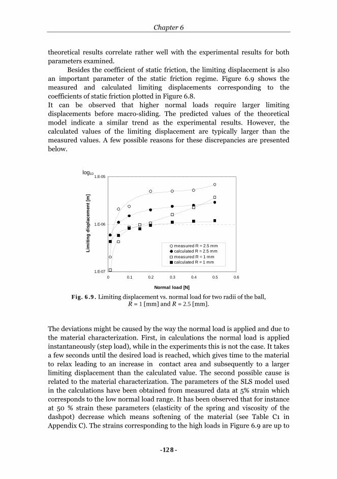
Chapter 6
-128-
theoretical results correlate rather well with the experimental results for both parameters examined. Besides the coefficient of static friction, the limiting displacement is also an important parameter of the static friction regime. Figure 6.9 shows the measured and calculated limiting displacements corresponding to the coefficients of static friction plotted in Figure 6.8. It can be observed that higher normal loads require larger limiting displacements before macro-sliding. The predicted values of the theoretical model indicate a similar trend as the experimental results. However, the calculated values of the limiting displacement are typically larger than the measured values. A few possible reasons for these discrepancies are presented below.
The deviations might be caused by the way the normal load is applied and due to the material characterization. First, in calculations the normal load is applied instantaneously (step load), while in the experiments this is not the case. It takes a few seconds until the desired load is reached, which gives time to the material to relax leading to an increase in contact area and subsequently to a larger limiting displacement than the calculated value. The second possible cause is related to the material characterization. The parameters of the SLS model used in the calculations have been obtained from measured data at 5% strain which corresponds to the low normal load range. It has been observed that for instance at 50 % strain these parameters (elasticity of the spring and viscosity of the dashpot) decrease which means softening of the material (see Table C1 in Appendix C). The strains corresponding to the high loads in Figure 6.9 are up to
1.E-07
1.E-06
1.E-05
0 0.1 0.2 0.3 0.4 0.5 0.6
Normal load [N]
Lim
iting
dis
plac
emen
t [m
]
measured R = 2.5 mmcalculated R = 2.5 mmmeasured R = 1 mmcalculated R = 1 mm
Fig. 6.9. Limiting displacement vs. normal load for two radii of the ball, R = 1 [mm] and R = 2.5 [mm].
log10
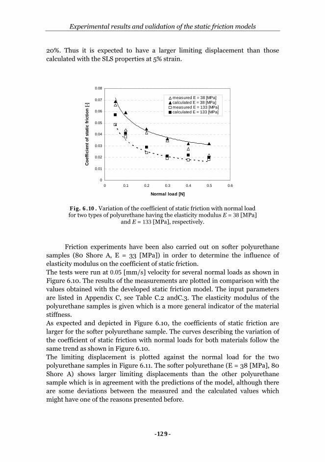
Experimental results and validation of the static friction models
-129-
20%. Thus it is expected to have a larger limiting displacement than those calculated with the SLS properties at 5% strain.
Friction experiments have been also carried out on softer polyurethane
samples (80 Shore A, E = 33 [MPa]) in order to determine the influence of elasticity modulus on the coefficient of static friction. The tests were run at 0.05 [mm/s] velocity for several normal loads as shown in Figure 6.10. The results of the measurements are plotted in comparison with the values obtained with the developed static friction model. The input parameters are listed in Appendix C, see Table C.2 andC.3. The elasticity modulus of the polyurethane samples is given which is a more general indicator of the material stiffness. As expected and depicted in Figure 6.10, the coefficients of static friction are larger for the softer polyurethane sample. The curves describing the variation of the coefficient of static friction with normal loads for both materials follow the same trend as shown in Figure 6.10. The limiting displacement is plotted against the normal load for the two polyurethane samples in Figure 6.11. The softer polyurethane (E = 38 [MPa], 80 Shore A) shows larger limiting displacements than the other polyurethane sample which is in agreement with the predictions of the model, although there are some deviations between the measured and the calculated values which might have one of the reasons presented before.
0
0.01
0.02
0.03
0.04
0.05
0.06
0.07
0.08
0 0.1 0.2 0.3 0.4 0.5 0.6
Normal load [N]
Coe
ffici
ent o
f sta
tic fr
ictio
n [-]
measured E = 38 [MPa]calculated E = 38 [MPa]measured E = 133 [MPa]calculated E = 133 [MPa]
Fig. 6.10. Variation of the coefficient of static friction with normal load for two types of polyurethane having the elasticity modulus E = 38 [MPa]
and E = 133 [MPa], respectively.

Chapter 6
-130-
6.2 Multi-asperity static friction measurements Friction experiments have been also carried out on a rough rubber surface in contact with a smooth metallic counter surface in order to validate the multi-asperity static friction model. The experimental set-up used for the friction tests is briefly described in the next section. Then the experimental results are discussed and compared with the theoretical predictions. 6.2.1 Experimental set-up Friction experiments have been performed on the tribometer shown in Figure 6.12. This equipment is suitable for carrying out experiments at relatively low pressure and very low velocities in a load-controlled contact situation. A description of the apparatus is provided below. The main parts of the tribometer are the normal force system, the friction force system and the specimen control system, as depicted in Figure 6.12. The normal force system comprises a piezo sensor and a piezo actuator and is able to apply and measure the normal load. This system is fixed on a lever by means of a coupling element which ensures the required stiffness in normal direction and flexibility in the other directions.
1.E-07
1.E-06
1.E-05
0 0.1 0.2 0.3 0.4 0.5 0.6
Normal load [N]
Lim
iting
dis
plac
emen
t [m
]
measured E = 38 [MPa]calculated E = 38 [MPa]measured E = 133 [MPa]calculated E = 133 [MPa]
Fig. 6.11. Variation of limiting displacement with normal load for two types of polyurethane having the elasticity modulus E = 38 [MPa] and E = 133 [MPa].
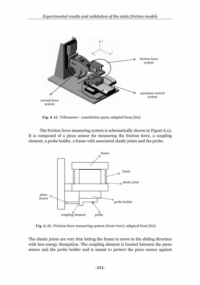
Experimental results and validation of the static friction models
-131-
The friction force measuring system is schematically shown in Figure 6.13. It is composed of a piezo sensor for measuring the friction force, a coupling element, a probe holder, a frame with associated elastic joints and the probe.
The elastic joints are very thin letting the frame to move in the sliding direction with less energy dissipation. The coupling element is located between the piezo sensor and the probe holder and is meant to protect the piezo sensor against
friction force system
specimen control system
normal forcesystem
Fig. 6.12. Tribometer– constitutive parts, adapted from [60].
Fig. 6.13. Friction force measuring system (front view), adapted from [60].
coupling element probe
elastic joint
beam
frame
piezo sensor
probe holder

Chapter 6
-132-
undesired potential moments which might occur during sliding. During a friction test the specimen is displaced by the moving table while the probe is fixed. The signal generated by the piezo sensor is recorded and converted in the final friction force signal.
The specimen control system is used for positioning of the specimen in x and y direction, for moving it in the sliding direction and to align it in order to have a plan parallel movement. The main parts of the control system are the linear positioning stage for x and y direction, the tilting table and the specimen. The specifications of the equipment are listed in Table 6.3.
Table 6.3 SFA specifications, from [60].
requested value realized value Parameter
range precision range precision
Normal force 0.1 ÷ 50 N 5 mN 0.1 ÷ 45 N 2 mN
Friction force 0.1 ÷ 50 N 5 mN 0.1 ÷ 50 N 0.5 mN
Sliding velocity 0 ÷ 20 mm/s 1 μm/s 0 ÷ 50 mm/s 1 μm/s
Sliding movement 0 ÷ 20 mm 1 μm 0 ÷ 50 mm 1 μm
Lateral movement 0 ÷ 20 mm 1 μm 0 ÷ 50 mm 1 μm
Vertical movement - coarse - fine
0 ÷ 50 mm 0 ÷ 200 μm
5 μm
10 nm
0.1 ÷ 50 N 0.1 ÷ 50 N
1 μm 9 μm
Experimental details
Friction between a rough rubber plate and a smooth spherical-ended steel sample has been investigated in order to validate the multi-asperity static friction model, see Figure 6.14. The spherical ended steel sample has a large radius R = 38.1 [mm] which results in almost a flat on flat contact (multi-asperity contact) with the rubber plate and prevents the occurrence of the edge effect.
Fn
vt R
Fig. 6.14. Friction tests configuration.
rough rubber
steel

Experimental results and validation of the static friction models
-133-
The surface roughness of the polyurethane (95 Shore A) sample has been measured with an interference microscope as previously explained in Chapter 3, for details see section 3.4.1.
The surface topography of the rubber specimen is shown in Figure 6.15. The measured height data were preprocessed and analyzed according to the procedure described by de Rooij [21], see also Chapter 3. The resulting surface parameters as well as the summit parameters are summarized in Table 6.4. The friction experiments were run at a low velocity of about 5 [μm/s], at 20°C and 25% humidity. Table 6.4 Surface and summit roughness parameters.
Material A [m2] Ra [μm] β [μm] σs [μm] η [m-2]
Polyurethane 95 Shore 8.85·10-7 0.24 28.6 0.51 5·109
6.2.2 Results Friction experiments were carried out in the configuration depicted in Figure 6.14. A recorded friction force vs. tangential displacement signal is illustrated in Figure 6.16 for an applied normal load of 0.5 [N].
From this figure it can be seen that the friction force increases quickly to a maximum value corresponding to the static friction and to the limiting displacement then falls to a stable value, the so-called dynamic friction force.
Fig. 6.15. Surface height data – polyurethane sample.
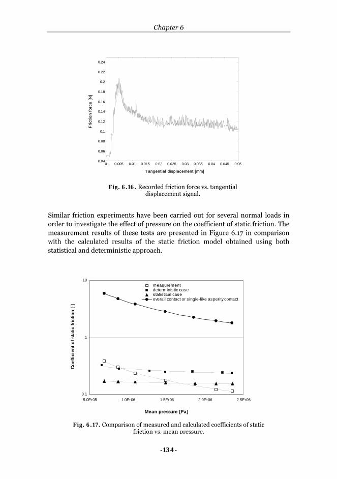
Chapter 6
-134-
Similar friction experiments have been carried out for several normal loads in order to investigate the effect of pressure on the coefficient of static friction. The measurement results of these tests are presented in Figure 6.17 in comparison with the calculated results of the static friction model obtained using both statistical and deterministic approach.
0 0.005 0.01 0.015 0.02 0.025 0.03 0.035 0.04 0.045 0.050.04
0.06
0.08
0.1
0.12
0.14
0.16
0.18
0.2
0.22
0.24
Fric
tion
forc
e [N
]
Tangential displacement [mm]
Fig. 6.16. Recorded friction force vs. tangential
displacement signal.
0.1
1
10
5.0E+05 1.0E+06 1.5E+06 2.0E+06 2.5E+06
Mean pressure [Pa]
Coef
ficie
nt o
f sta
tic fr
ictio
n [-]
measurementdeterministic casestatistical caseoverall contact or single-like asperity contact
Fig. 6.17. Comparison of measured and calculated coefficients of static
friction vs. mean pressure.

Experimental results and validation of the static friction models
-135-
Due to the convergence problems encountered in the actual algorithm the results using the deterministic approach with bulk deformation is not presented for this case. The input parameters used in the calculations are listed in Appendix C, Table C.4. Figure 6.17 indicates a decrease of the coefficient of static friction with pressure in the considered range for both measured and calculated curves. At low pressures the results obtained using the deterministic approach resemble well the measured values. Increasing the pressure, according to the deterministic contact model the adjacent asperities merge into larger equivalent asperities.
For instance in Figure 6.18 the local areas of the contacting asperities are plotted against the local loads for a total normal load of 2.1 [N] corresponding to a mean nominal contact pressure of 2.35 [MPa]. It can be observed that there is one large asperity denoted as “dominant” with a radius of 0.4 [mm] which carries almost the whole normal load and therefore will have the major contribution to the static friction force. Moreover, higher pressures imply larger bulk deformations which would result in smaller dominant asperities and, as a consequence, smaller coefficients of friction, see also Figure 5.20. This might be an explanation for the slower decreases of the coefficient of static friction compared with the experimental curve. The statistical approach underestimates the coefficient of static friction at low pressures. This is due to the assumption that all asperities have the same radius (mean radius) which is evaluated before the surfaces are in contact. This mean
10-6 10-5 10-4 10-3 10-2 10-1 100 10110-12
10-11
10-10
10-9
10-8
10-7
10-6
Local loads [N]
Loca
l con
tact
are
as [m
2 ]
d=1.0317e-006 [m]
“dominant” asperity
Fig. 6.18. Local contact areas vs. local loads for Fn = 2.1 [N]; “dominant asperity” which has the major contribution in the load carrying capacity and as
a result in the static friction force.

Chapter 6
-136-
radius β = 28.6 [μm] is smaller than the radius of the real asperities in contact. The deterministic model neglects the bulk deformation but takes into account real micro-contacts. The result is a good prediction of static friction at lower pressures. Assuming that there is overall contact between surfaces the single-asperity friction model can be used to calculate the coefficient of static friction. In this case the contact area is much larger than the real contact area determined by the contacting asperities or summits which results in a higher coefficient of static friction as shown in Figure 6.17. It can be concluded that, in this case, the system is clearly behaving as a multi-asperity contact.
In Figure 6.19 the measured values of the limiting displacement are presented in comparison with the calculated values for the same pressure range as in Figure 6.17. The values obtained using the deterministic approach with asperities are larger than the measured values. The statistical approach with summits underestimates the total limiting displacement due to the small mean summit radius. In the deterministic case the total limiting displacement is given by the limiting displacement of the dominant asperity. It has been shown in Chapter 5 that taking into account the bulk deformation results in smaller limiting displacements, which will shift the calculated values closer to the measured ones.
The results strongly indicate that the surface description plays a significant role in the static friction model. The statistical approach provides a low limit to the static friction model while the deterministic model determines the upper limit, as schematically shown in Figure 6.20.
0.0E+00
5.0E-06
1.0E-05
1.5E-05
2.0E-05
2.5E-05
3.0E-05
5.0E+05 7.0E+05 9.0E+05 1.1E+06 1.3E+06 1.5E+06 1.7E+06 1.9E+06 2.1E+06 2.3E+06 2.5E+06
Mean pressure [Pa]
Lim
iting
dis
plac
emen
t [m
]
measurementdeterministic case
statistical case
Fig. 6.19. Limiting displacement vs. mean pressure; comparison between
the measured and calculated values.

Experimental results and validation of the static friction models
-137-
Conclusively, the developed friction model predicts the static friction force and the limiting displacement using an appropriate description of the surface topography modeled as a multi-asperity contact. 6.3 Summary and conclusions In this chapter friction experiments carried out on rubber/steel specimens are presented. Single-asperity friction measurements have been performed on a nano-tribometer using a ball on flat configuration. The influence of normal load, geometry (radius of the ball) and rubber-like material stiffness on the coefficient of static friction and limiting displacement was experimentally investigated. The results of the tests were compared with the theoretical predictions. The results show a good correlation between the experimental results and the calculated values with respect to the variation of the coefficient of static friction with normal load and the radius of the ball. Larger radii of the ball result in higher coefficients of friction while higher normal loads determine smaller coefficients of friction. Conversely, the limiting displacement increases at higher loads and for larger radii of the ball. The coefficient of static friction decreases for “stiffer” materials, for instance polyurethane 95 Shore A (E = 133 MPa) compared with polyurethane 80 Shore A (E = 38 MPa). Then, friction between a rough polyurethane sample and a smooth steel counterpart has been investigated in order to validate the multi-asperity static friction model. For the pressure range considered, the coefficient of static friction decreases with higher pressures. A faster decline in the coefficient of static friction is observed
Statistical model – summits
Deterministic model – equivalent asperities
Real topography
Fig. 6.20. Modeling the surface topography: statistical approach and deterministic approach.
Chapter 6
-138-
in the experimental curve compared with the calculated curves. The deterministic approach, in which surface roughness is modeled by equivalent asperities, departs from the experimental predictions at higher pressures. This might be explained by the merging of adjacent asperities into larger “dominant asperities” which overestimate the real ones because the bulk deformation is not taken into account. The statistical approach, which uses summits that follow a Gaussian distribution, predicts smaller coefficients of static friction at lower pressure than the measured values. This is caused by the constant radius of the summits which is evaluated from the surface roughness measurements before the surfaces are brought in contact and underestimates the real values of “extreme summits”. Nevertheless, the values of the coefficient of static friction and certainly the physical effect are predicted well by the developed static friction model. Conclusively, the developed single-asperity friction model predicts very well the static friction force while the limiting displacement is in rather good agreement with the experiments. The multi-asperity friction model, which comprises a statistical and a deterministic contact model, provides good estimations for the coefficient of static friction as well as for the limiting displacement.
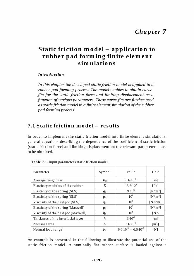
-139-
Chapter 7
Static friction model – application to rubber pad forming finite element
simulations
Introduction
In this chapter the developed static friction model is applied to a rubber pad forming process. The model enables to obtain curve-fits for the static friction force and limiting displacement as a function of various parameters. These curve-fits are further used as static friction model in a finite element simulation of the rubber pad forming process.
7.1 Static friction model – results In order to implement the static friction model into finite element simulations, general equations describing the dependence of the coefficient of static friction (static friction force) and limiting displacement on the relevant parameters have to be obtained.
Table 7.1. Input parameters static friction model.
Parameter Symbol Value Unit
Average roughness Ra 0.6·10-6 [m]
Elasticity modulus of the rubber E 13.6·106 [Pa]
Elasticity of the spring (SLS) g1 9·106 [N/m2]
Elasticity of the spring (SLS) g2 108 [N/m2]
Viscosity of the dashpot (SLS) η1 109 [N·s/m2
Elasticity of the spring (Maxwell) g3 107 [N/m2]
Viscosity of the dashpot (Maxwell) η2 106 [N·s
Thickness of the interfacial layer h 3·10-7 [m]
Nominal area A 6.6·10-8 [m2]
Normal load range Fn 6.6·10-5 - 6.6·10-2 [N]
An example is presented in the following to illustrate the potential use of the static friction model. A nominally flat rubber surface is loaded against a
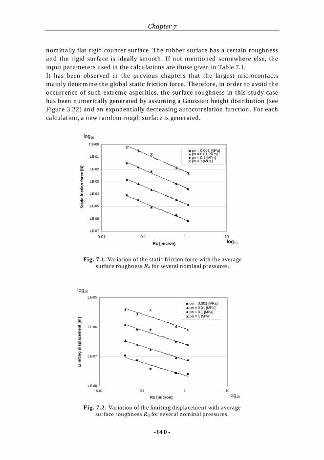
Chapter 7
-140-
nominally flat rigid counter surface. The rubber surface has a certain roughness and the rigid surface is ideally smooth. If not mentioned somewhere else, the input parameters used in the calculations are those given in Table 7.1. It has been observed in the previous chapters that the largest microcontacts mainly determine the global static friction force. Therefore, in order to avoid the occurrence of such extreme asperities, the surface roughness in this study case has been numerically generated by assuming a Gaussian height distribution (see Figure 3.22) and an exponentially decreasing autocorrelation function. For each calculation, a new random rough surface is generated.
Fig. 7.1. Variation of the static friction force with the average surface roughness Ra for several nominal pressures.
1.E-07
1.E-06
1.E-05
1.E-04
1.E-03
1.E-02
1.E-01
1.E+00
0.01 0.1 1 10Ra [micron]
Stat
ic fr
ictio
n fo
rce
[N]
pn = 0.001 [MPa]pn = 0.01 [MPa]pn = 0.1 [MPa]pn = 1 [MPa]
log10
log10
Fig. 7.2. Variation of the limiting displacement with average surface roughness Ra for several nominal pressures.
1.E-08
1.E-07
1.E-06
1.E-05
0.01 0.1 1 10
Ra [micron]
Lim
iting
dis
plac
emen
t [m
]
pn = 0.001 [MPa]pn = 0.01 [MPa]pn = 0.1 [MPa]pn = 1 [MPa]
log10
log10

Static friction model – application to rubber pad forming finite element simulations
-141-
It has been shown in Chapter 5 that surface roughness does influence the static friction force and the limiting displacement. In Figure 7.1 the surface roughness has been varied by modifying the average surface roughness Ra. The calculations have been done for a certain nominal pressure range. For the material and surface parameters considered, the static friction force as well as the limiting displacement increase at higher nominal pressures, while they decrease by increasing the surface roughness expressed by Ra, see Figures 7.1 and 7.2. Two equations can be obtained inferred from the results presented in Figures 7.1 and 7.2. First, the dependence of static friction force on surface roughness Ra and nominal pressure is given by
41−28110− ⋅⋅10= ..ans RpF (7.1)
with Ra in [µm] and pn in [Pa]. Second, the liming displacement as a function of surface roughness and nominal pressure reads:
450−55010− ⋅⋅10⋅5= ..anl Rpδ (7.2)
These equations provide input data with respect to static friction for finite element simulation of the rubber pad forming processes.
The influence of the material in terms of “elasticity modulus” of the rubber on the static friction force and limiting displacement is shown in Figures 7.3 and 7.4.
1.E-10
1.E-09
1.E-08
1.E-07
1.E-06
1.E-05
1.E-04
1.E-03
1.E-02
1.E-01
1.E+00
1 10 100 1000
Elasticity modulus [MPa]
Stat
ic fr
ictio
n fo
rce
[N]
pn = 0.001 [MPa]pn = 0.01 [MPa]pn = 0.1 [MPa]pn = 1 [MPa]
log10
Fig. 7.3. Variation of the static friction force with the elasticity modulus E at several nominal pressures.
log10
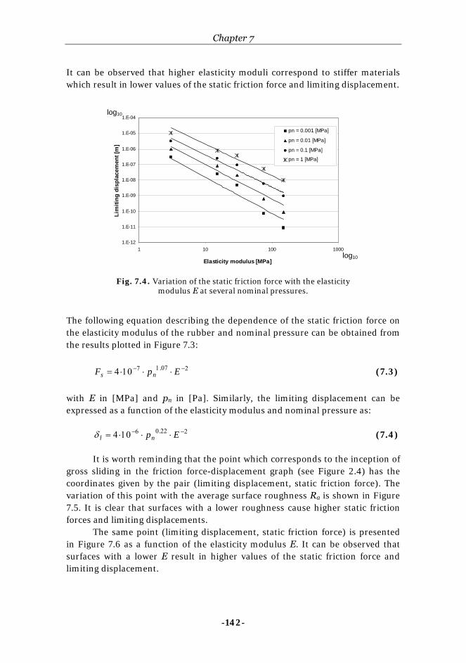
Chapter 7
-142-
It can be observed that higher elasticity moduli correspond to stiffer materials which result in lower values of the static friction force and limiting displacement.
The following equation describing the dependence of the static friction force on the elasticity modulus of the rubber and nominal pressure can be obtained from the results plotted in Figure 7.3:
2−0717− ⋅⋅10⋅4= EpF ns. (7.3)
with E in [MPa] and pn in [Pa]. Similarly, the limiting displacement can be expressed as a function of the elasticity modulus and nominal pressure as: 2−2206− ⋅⋅10⋅4= Epnl
.δ (7.4)
It is worth reminding that the point which corresponds to the inception of gross sliding in the friction force-displacement graph (see Figure 2.4) has the coordinates given by the pair (limiting displacement, static friction force). The variation of this point with the average surface roughness Ra is shown in Figure 7.5. It is clear that surfaces with a lower roughness cause higher static friction forces and limiting displacements.
The same point (limiting displacement, static friction force) is presented in Figure 7.6 as a function of the elasticity modulus E. It can be observed that surfaces with a lower E result in higher values of the static friction force and limiting displacement.
1.E-12
1.E-11
1.E-10
1.E-09
1.E-08
1.E-07
1.E-06
1.E-05
1.E-04
1 10 100 1000
Elasticity modulus [MPa]
Lim
iting
dis
plac
emen
t [m
]
pn = 0.001 [MPa]
pn = 0.01 [MPa]
pn = 0.1 [MPa]
pn = 1 [MPa]
log10
log10
Fig. 7.4. Variation of the static friction force with the elasticity modulus E at several nominal pressures.

Static friction model – application to rubber pad forming finite element simulations
-143-
The effect of nominal pressure on the static friction force vs. limiting displacement is shown in Figure 7.7. Both static friction force and limiting displacement increase at high nominal pressures.
0.0E+00
2.0E-04
4.0E-04
6.0E-04
8.0E-04
1.0E-03
1.2E-03
1.4E-03
1.6E-03
0.0E+00 5.0E-08 1.0E-07 1.5E-07 2.0E-07 2.5E-07 3.0E-07 3.5E-07 4.0E-07
Limiting displacement [m]
Stat
ic fr
ictio
n fo
rce
[N]
Ra↓
Fig. 7.5. Static friction force vs. limiting displacement as a function of average surface roughness Ra.
1.E-08
1.E-07
1.E-06
1.E-05
1.E-04
1.E-03
1.E-11 1.E-10 1.E-09 1.E-08 1.E-07 1.E-06
Limiting displacement [m]
Sta
tic fr
ictio
n fo
rce
[N]
E↓
Fig. 7.6. Static friction force vs. limiting displacement as a function of elasticity modulus E.
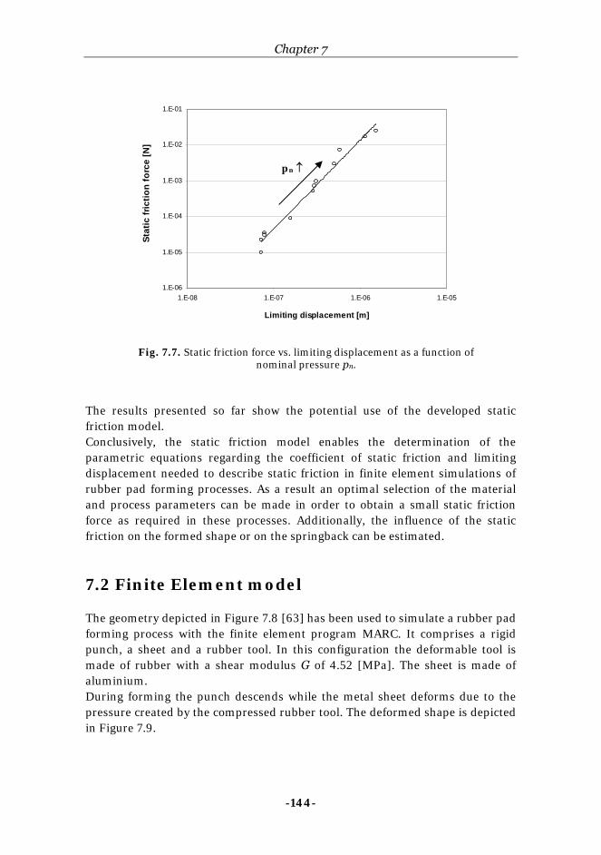
Chapter 7
-144-
The results presented so far show the potential use of the developed static friction model. Conclusively, the static friction model enables the determination of the parametric equations regarding the coefficient of static friction and limiting displacement needed to describe static friction in finite element simulations of rubber pad forming processes. As a result an optimal selection of the material and process parameters can be made in order to obtain a small static friction force as required in these processes. Additionally, the influence of the static friction on the formed shape or on the springback can be estimated.
7.2 Finite Element model The geometry depicted in Figure 7.8 [63] has been used to simulate a rubber pad forming process with the finite element program MARC. It comprises a rigid punch, a sheet and a rubber tool. In this configuration the deformable tool is made of rubber with a shear modulus G of 4.52 [MPa]. The sheet is made of aluminium. During forming the punch descends while the metal sheet deforms due to the pressure created by the compressed rubber tool. The deformed shape is depicted in Figure 7.9.
1.E-06
1.E-05
1.E-04
1.E-03
1.E-02
1.E-01
1.E-08 1.E-07 1.E-06 1.E-05
Limiting displacement [m]
Stat
ic fr
ictio
n fo
rce
[N]
pn ↑
Fig. 7.7. Static friction force vs. limiting displacement as a function of nominal pressure pn.

Static friction model – application to rubber pad forming finite element simulations
-145-
The radius of curvature denoted Rf of the formed strip is one of the parameters which is industrially the most relevant. Thus, this radius Rf is investigated for two cases. First, the rubber pad forming process is simulated using a Coulomb friction, i.e. constant coefficient of static friction with μ = 0.3. Second, the coefficient of static friction is taken as a function of nominal pressure, average roughness and elasticity modulus of the rubber as predicted by the developed
rubber tool
metal sheet punch
Fig. 7.8. Finite element model – geometry, adapted from [63].
Fig. 7.9. Deformation of the metal sheet and rubber tool due to the descending of the punch, adapted from [63].

Chapter 7
-146-
static friction model. In this example Ra = 0.3 [μm] and E = 13.56 [MPa], resulting in μ = 0.0082 · pn
0.28. In the FEM model, the preliminary displacement is not taken as a function of pressure for reasons of simplicity.
The resulting geometry of the strip is shown in Figure 7.10 for the two cases considered. A difference in the radius of curvature Rf of the formed strip can be noticed. The fitted radius Rf is about 28.1 [mm] for the case when Coulomb friction is used (case 1). If the developed static friction model is used instead, the radius of curvature Rf is 27.4 [mm] (case 2). This difference is more pronounced for a rubber pad surface with a low roughness. In this case the coefficient of static friction can reach relatively high levels.
Fig. 7.10. Resulting geometry of the strip: case 1 – Coulomb friction;
case 2 - developed static friction model, adapted from [63].
case 2
case 1
Rf

Static friction model – application to rubber pad forming finite element simulations
-147-
7.3 Summary and conclusions The developed static friction model is applied to a rubber pad forming process. Curve-fits can be obtained from the developed model for the static friction force (coefficient of static friction) and limiting displacement as a function of various parameters. These data are used as input parameters in the finite element simulation of rubber pad forming processes. An example of a finite element simulation of a rubber pad forming process is shown in this chapter. A Coulomb friction model and the developed static friction model are used in the simulations and then compared. The results of the simulations show that by using the static friction model instead of the very often applied Coulomb friction model has a significant effect on the radius of curvature of the formed strip. The surface roughness of the rubber pad will influence to a large extent the geometry of the strip due to its effect on the friction level.

Chapter 7
-148-
-149-
Chapter 8
Conclusions and recommendations
8.1. Conclusions
The theoretical modeling and experimental investigations of static friction in rubber/metal contact have been presented in the previous chapters. The main conclusions of the research are summarized in this section. Chapter 2 - literature survey
• The main characteristic parameters of the static friction regime are the static friction force and the limiting displacement. • Two temperature-related static friction mechanisms have been reported in the literature for the contact between metallic surfaces, namely the creep of asperities at low temperatures and welding of asperities at higher temperatures. • As a result of the experimental evidence, Mindlin’s approach of a contact area comprising a stick and a slip zone, which evolve until gross sliding occurs, has been chosen to describe the mechanism of static friction between rubber and metal bodies in contact. • Experimental results reported in the literature showed that the static friction regime in contact of metallic as well as rubber surfaces depends on several parameters as pressure, dwell time, temperature, and surface topography. Chapter 3 - Contact of surfaces in rubber pad forming processes
• The relevant properties of the contacting bodies in rubber pad forming processes in terms of mechanical properties, surface energy and roughness have been determined. • Depending on the ratio of real contact area to nominal contact area, different approaches can be used to model the contact of real bodies. When the contact area is a small fraction of the nominal contact area, a multi-summit model (for instance Greenwood-Williamson) is appropriate. At the other extreme, when the real contact area almost equals the nominal contact area, a single (macro) asperity model is suitable. The intermediate case can be modeled using a multi-asperity contact which takes into account the asperity interaction and the bulk deformation.

Chapter 8
-150-
Chapter 4 – Single asperity static friction model
• A single-asperity static friction model has been developed for rubber/metal contacts. In this model, friction is attributed to the shear of a thin interfacial layer. • A mechanism similar to that described in Mindlin’s theory is assumed to take place in rubber-metal asperity contact. • The viscoelastic behaviour of the rubber bulk is incorporated into the static friction model by using a mechanical model. A method has been developed for quantifying the parameters of the mechanical model. • At low loads adhesion plays a significant role. Therefore, it has been modeled by a modified JKR theory, which takes into account the viscoelastic behavior of the rubber. • A parametric study is presented regarding the influence of several parameters such as normal load, material parameters, geometry (radius of the sphere), thickness of the interfacial layer on the static friction force (coefficient of static friction) as well as on the preliminary displacement. • The results of calculations indicate that small coefficients of static friction correspond to large normal loads (or contact pressures), small radii of asperities, and to thick interfacial layers. The limiting displacement is larger for high normal loads, large asperities and thin interfacial layers. Chapter 5 – Multi asperity static friction model
• A multi-asperity static friction model has been developed based on the behavior of individual micro-contacts. • Two approaches have been used to model the contact between a viscoelastic surface and rigid flat. The statistical or multi-summit approach offers a simplified solution, based on independent summits. The multi-asperity or deterministic model is a more realistic approach which takes into account merging of asperities at larger loads as well as the bulk deformation. • The deterministic approach predicts larger static friction forces and limiting displacements than the statistical approach. • The global frictional behavior depends on the friction force of individual asperities and is mainly determined by a few large microcontacts. This means that the microgeometry of the surface is the decisive factor for the frictional behavior. • An accurate multi-asperity model is therefore very important for a good prediction of friction. • In general, rougher surfaces result in smaller coefficients of static friction. Chapter 6 – Experimental results and validation of the static friction models
• Friction experiments have been carried out on rubber/steel specimens in order to validate the static friction models.
Conclusions and recommendations
-151-
• Single-asperity friction measurements have been performed on a nano-tribometer using a ball on flat configuration. The influence of normal load, geometry (radius of the ball) and stiffness of the rubber on the coefficient of static friction and limiting displacement was experimentally investigated. • The results show a good agreement between the experimental results and the calculated values with respect to the coefficient of static friction. Larger radii of the ball result in higher coefficients of friction while higher normal loads determine smaller coefficients of friction. Conversely, the limiting displacement increases at higher loads and for larger radii of the ball. The coefficient of static friction decreases for “stiffer” materials. • Friction between a rough polyurethane sample and a smooth steel counterpart (multi-asperity contact) was experimentally investigated in order to validate the multi-asperity static friction model. • For the pressure range considered, the coefficient of static friction decreases with higher pressures. A faster decline in the coefficient of static friction is observed in the experimental curve compared with the calculated curves. • The deterministic approach without bulk deformation overestimates the experimental predictions at higher pressures. This is explained by the merging of adjacent asperities into larger “dominant asperities” in the model which overestimate the size of the microcontacts. • The statistical approach underestimates the coefficient of static friction at lower pressures. This is caused by an underestimation of the size of the microcontacts in the model. Nevertheless, the values of the coefficient of static friction and certainly the physical effect are predicted well by the developed static friction model. • The developed single-asperity friction model predicts very well the static friction force while the limiting displacement is in good agreement with the experiments. The multi-asperity friction model, which comprises a statistical and a deterministic contact model, provides good estimations for the coefficient of static friction as well as for the limiting displacement. Chapter 7 – Static friction model with application to rubber pad forming finite element simulations
• The developed static friction model is applied to a rubber pad forming process. • Curve-fits can be obtained from the multi-asperity model for the static friction force (coefficient of static friction) and limiting displacement as a function of various parameters. These data are used as input parameters in the finite element simulation of a rubber pad forming process. • An example of a finite element model describing a rubber pad forming process is shown. A Coulomb friction model and the developed static friction model are used in the simulations. The results reveal that a low level of the coefficient of static friction, as predicted by the static friction model for rough surfaces, slightly influences the finite element simulations with respect to the radius of
Chapter 8
-152-
curvature of the formed strip. If the roughness of the rubber pad is lower, it is expected that the predicted curvature of the formed strip will be significantly influenced by the chosen model.
8.2 Recommendations • It is recommended that for the case of a rough rigid surface contacting the rubber, the ploughing component to be investigated. • The ploughing component can be studied experimentally by using the reverse configuration, a rigid ball pressed against a viscoelastic flat. Besides this, a suitable model should be developed. • The viscoelastic behavior of the rubber has been modeled by a relatively simple mechanical model (Standard Linear Solid). Complex models can describe the viscoelastic behavior of rubber more accurately. For instance, the viscoelastic behavior of rubber should be modeled as strain dependent. • A Maxwell model has been used to describe the properties of the interfacial layer. Indentation tests can be used in the future to characterize the surface layers experimentally. • In order to be able to compare accurately the results of the friction experiments with the theoretical results in a load-controlled case, the history of the normal load has to be known. This means that the real load path has to be used in the calculations instead of the step load function. This will lead to complex solutions, which are analytically non-tractable. • The algorithm used in the multi-asperity contact has to be improved in order to converge for a wide range of the input parameters when bulk deformation is taken into account.
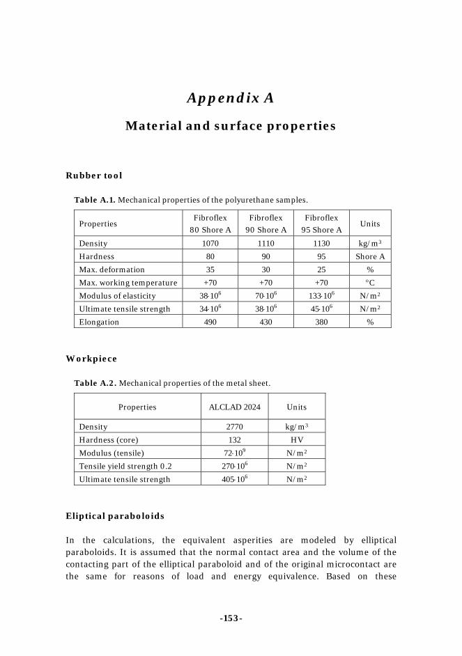
-153-
Appendix A
Material and surface properties Rubber tool
Table A.1. Mechanical properties of the polyurethane samples.
Properties Fibroflex
80 Shore A
Fibroflex
90 Shore A
Fibroflex
95 Shore A Units
Density 1070 1110 1130 kg/m3
Hardness 80 90 95 Shore A
Max. deformation 35 30 25 %
Max. working temperature +70 +70 +70 °C
Modulus of elasticity 38⋅106 70⋅106 133⋅106 N/m2
Ultimate tensile strength 34⋅106 38⋅106 45⋅106 N/m2
Elongation 490 430 380 %
Workpiece
Table A.2. Mechanical properties of the metal sheet.
Properties ALCLAD 2024 Units
Density 2770 kg/m3
Hardness (core) 132 HV
Modulus (tensile) 72⋅109 N/m2
Tensile yield strength 0.2 270⋅106 N/m2
Ultimate tensile strength 405⋅106 N/m2
Eliptical paraboloids In the calculations, the equivalent asperities are modeled by elliptical paraboloids. It is assumed that the normal contact area and the volume of the contacting part of the elliptical paraboloid and of the original microcontact are the same for reasons of load and energy equivalence. Based on these
Appendix A
-154-
assumptions, the equivalent paraboloid is defined by the radius Rx in x direction and radius Ry in y direction which are given by:
aspasp
aspx V
AR
λπ ⋅⋅⋅=
4
2
(A.1)
2mxy RR λ⋅= (A.2)
where Aasp is the measured contact area of asperity, Vasp is the asperity volume and λasp is the ellipticity ratio of asperity [23]. The height of the equivalent asperity has been determined by Jamary [62] and is given by equation
x
x
offcut R
L
hz22
2
⎟⎠
⎞⎜⎝
⎛
+= − (A.3)
where hcut-off is the contact separation or the cut-off of contacting surfaces, Lx is the diameter of the cross-sectional elliptical contact area in x direction.

-155-
Appendix B
Single-asperity static friction model B.1 Normal contact of a viscoelastic sphere with a rigid flat In a load-controlled case it is considered that the normal load varies in time according to ( ) ( )tHFtF nn ⋅= (B.1)
where t is the time and H(t) is the Heaviside step function or the unit step function defined as:
⎩⎨⎧
>
==
010tfor0
)(tfor
tH (B.2)
For t > 0 the contact radius av can be written as
( ) ( )3
83 tFR
ta nv
ϕ⋅⋅⋅= (B.3)
and the pressure distribution is expressed
( ) ( ) ( )22
322 )(
231)(4, rta
taF
trta
Rtrp v
v
nvv −⋅
⋅⋅
⋅=⋅−⋅
⋅=
πϕπ (B.4)
In a displacement-controlled case, the normal displacement or indentation is taken as ( ) ( )tHt nn ⋅= δδ (B.5)
In this case the contact radius is constant and equal to
[ ] 2/1nv Ra δ⋅= (B.6)

Appendix B
-156-
while the pressure distribution and normal load changes in time according to
( ) 224),( ratR
trp vv −⋅⋅⋅
= ψπ
(B.7)
( ) 3⋅⋅⋅38
= vn atR
tF ψ)( (B.8)
B.2 Normal contact including adhesion of a viscoelastic sphere with a rigid flat (modified JKR theory) The modified equations of the JKR theory are presented for a viscoelastic-rigid couple in a load-controlled case. The applied normal load is given by equation (B.1). For t > 0 the following equations give the contact radius a1v, the apparent normal load Fn1 and the pressure distribution p1v(r) when adhesion is taken into account:
( ) ( )3 11 8
3nv FtRta ⋅
⋅⋅=
ϕ (B.9)
( )2121 363 RWFRWRWFF vnvnn ⋅⋅⋅+⋅⋅⋅⋅+⋅⋅⋅+= πππ (B.10)
( ) ( ) ( )( ) 22
131
122
11
11 2
312
)( rtata
F
rtataFF
rp vv
n
vv
nnv −⋅
⋅⋅
⋅−
−⋅
⋅⋅−
=ππ
(B.11)
where Wv is the viscoelastic work of adhesion (see equation 4.24), Fn1 is the apparent Hertzian load which would determine a contact radius a1v. The pressure distribution p1v(r) comprises a tensile zone close to the edge of the contact area and a central compressive part whose radius acv is given by:
( ) ( )1
11 3
−+1⋅=
n
nnvcv F
FFtata (B.12)
Similarly, the equations which apply in a displacement-controlled case can be determined by replacing the elastic constant in the elastic solution (JKR theory) by the relaxation function ψ(t).
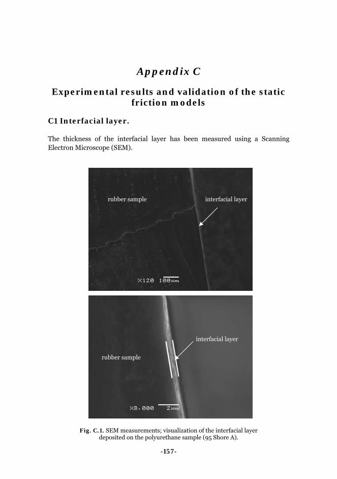
-157-
Appendix C
Experimental results and validation of the static friction models
C1 Interfacial layer. The thickness of the interfacial layer has been measured using a Scanning Electron Microscope (SEM).
Fig. C.1. SEM measurements; visualization of the interfacial layer deposited on the polyurethane sample (95 Shore A).
rubber sample
interfacial layer
interfacial layer rubber sample

Appendix C
-158-
A very thin layer of chromium (about 30 nm) has been deposited on the polyurethane surface. The visualization of the interfacial layer is shown in Figure C.1 for two magnifications, x120 and x8000. The thickness of the interfacial layer was measured on few polyurethane samples 95 Shore A. The measurements indicated values in the range 0.1 ÷ 0.8 [μm]. C.2 Single-asperity friction results C.2.1 Tangential load vs. time at various normal loads
In the single-asperity static friction model one of the input parameters is an increasing tangential load Ft(t) which is applied until macro-sliding occurs. In order to validate the theoretical model this function Ft(t) has to be determined.
The experimental curves, which were obtained on the nano tribometer, are fitted in Figure C.2 for several normal loads. The results indicate that the tangential load is an exponential function of time, Ft = c1· tc2 with c1 ranging from 4.8·10-4 to 7.6·10-4 and c2 from 1 to 1.3. C.2.2 Influence of the strain on the parameters of the Standard Linear Solid In order to determine the parameters of the Standard Linear Solid model, which describes the viscoelastic behavior of rubber, relaxation tests have been performed on the polyurethane samples. A comprehensive description of these
0
0.05
0.1
0.15
0.2
0 20 40 60 80 100
Time [s]
Tang
entia
l for
ce [N
]
Fn = 10 mNFn = 50 mN
Fn = 100 mNFn = 300 mNFn = 500 mN
Fig. C.2. Applied tangential force vs. time (fitted curves) at various normal loads.
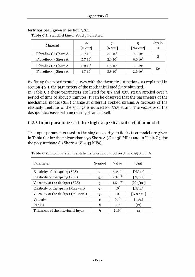
Appendix C
-159-
tests has been given in section 3.2.1. Table C.1. Standard Linear Solid parameters.
Material g1
[N/m2]
g2
[N/m2]
η
[N·s/m2]
Strain
%
Fibroflex 80 Shore A 2.7⋅107 3.1⋅108 7.6⋅109 Fibroflex 95 Shore A 5.7⋅107 2.1⋅108 8.6⋅109
5
Fibroflex 80 Shore A 6.8⋅106 5.5⋅107 1.8⋅199 Fibroflex 95 Shore A 1.7⋅107 5.9⋅107 2.2⋅109 50
By fitting the experimental curves with the theoretical functions, as explained in section 4.2.1, the parameters of the mechanical model are obtained. In Table C.1 these parameters are listed for 5% and 50% strain applied over a period of time of about 3 minutes. It can be observed that the parameters of the mechanical model (SLS) change at different applied strains. A decrease of the elasticity modulus of the springs is noticed for 50% strain. The viscosity of the dashpot decreases with increasing strain as well. C.2.3 Input parameters of the single-asperity static friction model The input parameters used in the single-asperity static friction model are given in Table C.2 for the polyurethane 95 Shore A (E = 138 MPa) and in Table C.3 for the polyurethane 80 Shore A (E = 33 MPa).
Table C.2. Input parameters static friction model– polyurethane 95 Shore A.
Parameter Symbol Value Unit
Elasticity of the spring (SLS) g1 6.4·107 [N/m2]
Elasticity of the spring (SLS) g2 2.3·108 [N/m2]
Viscosity of the dashpot (SLS) η1 1.5·109 [N·s/m2]
Elasticity of the spring (Maxwell) g3 107 [N/m2]
Viscosity of the dashpot (Maxwell) η2 106 [N·s /m2]
Velocity v 10-5 [m/s]
Radius R 10-3 [m]
Thickness of the interfacial layer h 2·10-7 [m]

Appendix C
-160-
Table C.3. Input parameters static friction model– polyurethane 80 Shore A.
Parameter Symbol Value Unit
Elasticity of the spring (SLS) g1 3.1·107 [N/m2]
Elasticity of the spring (SLS) g2 2.4·108 [N/m2]
Viscosity of the dashpot (SLS) η1 9.7·109 [N·s/m2]
Elasticity of the spring (Maxwell) g3 106 [N/m2]
Viscosity of the dashpot (Maxwell) η2 105 [N·s /m2]
Velocity v 5·10-5 [m/s]
Radius R 10-3 [m]
Thickness of the interfacial layer h 2·10-7 [m]
C.3 Multi-asperity friction results The results of the friction experiments carried out on the rough polyurethane surfaces against the smooth metallic counter surfaces were compared in section 6.2.2 with the prediction of the theoretical friction model. The input parameters used in the calculations are listed in Table C.4. For this polyurethane sample the thickness of the interfacial layer was about 0.7 [μm].
Table C.4 Values of the input parameters.
Parameter Symbol Value Unit
Elasticity of the spring (SLS model) g1 6.4·107 [N/m2]
Elasticity of the spring (SLS model) g2 2.3·108 [N/m2]
Viscosity of the dashpot (SLS model) η1 1.5·109 [N·s/m2]
Elasticity of the spring (Maxwell g3 107 [N/m2]
Viscosity of the dashpot (Maxwell η2 106 [N·s/m2]
Thickness of the interfacial layer hi 0.7·10-6 [m]
Nominal area An 8.85·10-7 [m2]
Velocity v 5·10-6 [m/s]

-161-
Bibliography [1] Dowson, D., History of Tribology, Professional Engineering Publishing Limited, London and Bury St Edmunds, UK, 1998, ISBN [2] Johnson, K.L., Surface interaction between elastically loaded bodies under tangential forces, Proceedings of the Royal Society of London, Series A, Mathematical and Physical Sciences, Vol. 230, Issue 1183, 1955, 531-548. [3] Mindlin, R.D., Compliance of elastic bodies in contact, ASME Journal of Applied Mechanics, Vol. 16, 1949, 259-268. [4] Chang, W.R., Etsion, I., Bogy, D.B., Static friction coefficient model for metallic rough surfaces, Journal of Tribology, Vol. 110, 1988, 57-61. [5] Persson, B.N.J., Albohr, O., Mancosu, F., Peveri, V., Samoilov, V.N., Sivebaek, I.M., On the nature of the static friction, kinetic friction and creep, Wear, Vol. 254, 2003, 835-851. [6] Galligan, J.M., McCullough, P., On the nature of static friction, Wear, Vol. 105, 1985, 337-340. [7] Nolle, H., Richardson, R.S.H., Static friction coefficients for mechanical and structural joints, Wear, Vol. 28, 1974, 1-13. [8] Broniec, Z., Lenkiewicz, W., Static friction processes under dynamic loads and vibration, Wear, Vol. 80, 1982, 261-271. [9] Roberts, A.D., Thomas, A.G., Static friction of smooth clean vulcanized rubber, NR Technology, Vol. 7, Part 2, 1976, 38-42. [10] Barquins, M., Adherence, friction and wear of rubber-like materials, Wear, Vol. 158, 1992, 87-117. [11] Barquins, M., Roberts, A.D., Rubber friction variation with rate and temperature: some new observations, J. Phys. D: Appl. Phys., Vol. 19, 1986, 547-563. [12] Tarr, W.R., Rhee, S.K., Static friction of automotive friction materials, Wear, Vol. 33, 1975, 373-375. [13] Bogdanovich, P.N., Baidak, A.A., Micro-slip in metal-polymer friction pairs, Journal of friction and wear, Vol. 23, No. 3, 2002, 41-45. [14] Adachi, K., Kato, K., Liu, J., Kawamura, H., The effect of contact morphology on initiation and propagation of micro-slip at contact interface, Proceedings of TRIB 2004, ASME/STLE International Joint Tribology Conference, 2004. [15] Hagman, L.A., Olofsson, U., A model for micro-slip between flat surfaces based on deformation of ellipsoidal elastic asperities – parametric study and experimental investigation, Tribology International, Vol. 31, No. 4, 1998, 209-217.

Bibliography
-162-
[16] Brockley, C.A., Davis, H.R., The time dependence of static friction, Journal of Lubrication Technology, Vol. 90, 1968, 35-41. [17] Kato, S., Sato, N., Matsubayashi, T., Some consideration on characteristics of the static frition of machine tool slideway, Journal of Lubrication Technology, Vol. 94, 1972, 234-247. [18] Johnson, K.L., Contact mechanics, Cambridge University Press, Cambridge, 1985, ISBN 052125576 7. [19] Bhusan, B., Introduction to tribology, John Wiley & Sons, New York, 2002, ISNB 0471 158933. [20] Greenwood, J.A., Williamson, J.B.P., Contact of nominally flat surfaces, Proceedings of the Royal Society of London. Series A, Mathematical and Physical Science, Vol. 295, Issue 1442, 1966, 300-319. [21] de Rooij, M.B., Tribological aspects of unlubricated deepdrawing processes, PhD thesis, University of Twente, 1998, ISBN 90365 12182. [22] de Rooij, M.B., private communication. [23] Masen, M. Abrasive tool wear in metal forming processes, PhD thesis, University of Twente, 2004, ISBN 9036520614. [24] Barquins, M., Friction and wear of rubber-like materials, Wear, Vol. 160, Issue 1, 1993, 1-11. [25] McFarlane, J.S., Tabor, D., Relation between friction and adhesion, Proceedings of the Royal Society of London. Series A, Mathematical and Physical Science, Vol. 202, Issue 1069, 1950, 244-253. [26] Courtney-Pratt, J.S., Eisner, E., The effect of a tangential force on the contact of metallic bodies, Proceedings of the Royal Society of London. Series A, Mathematical and Physical Science, Vol. 238, Issue 1215, 1950, 529-550. [27] Thiruvarudchelvan, S., Elastomers in metal forming: a review, Journal of Materials Processing Technology, Vol. 39, 1993, 88-82. [28] Ferry, J.D., Viscoelastic properties of polymers, John Wiley&Sons, Inc., New York, 1970. [29] http://en.wikipedia.org/wiki/Soap_bubble#Surface_tension_and_shape [30] Skvarla, J., Hydrophobic interaction between macroscopic and microscopic surfaces. Unification using surface thermodynamics, Advances in Colloid and Interface Science, Vol. 91, 2001, 335-390. [31] Balkenende, A.R., Boogaard, H.J.A.P., Scholten, M., Willard, N.P., Evaluation of different approaches to assess the surface tension of low-energy solids by means of contact angle measurements, Langmuir, Vol.14, 1998, 5907-5912. [32] Chibowski, E., Surface free energy of a solid from contact angle hysteresis, Advances in Colloid and Interface Science, Vol. 103, 2003, 149-172. [33] Radelczuk, H., Holysz, L., Chibowski, E., Comparison of the Lifshitz-van der Waals /acid-base and contact angle hysteresis approaches for determination of solid surface free energy, J. Adhesion Sci. Technol., Vol.16, 2002, 1547-1568.

Bibliography
-163-
[34] Moore, D.F., The friction and lubrication of elastomers, Pergamon Press, 1972. [35] Hertz, H., 1881, Über die Berührung fester elastischer Körper, Journal für die reine und angewandte Mathematik, Vol. 92, 1881, 156-171. [36] Hill, R.M., Dissado, L.A., Temperature dependence of relaxation processes, Journal of Physics C: Solid State Physics, Vol. 15, 1982, 5171-5193. [37] http://www.aircraftspruce.com/catalog/mepages/aluminfo.php [38] Adamson, A.W., Gast, A.P., Physical Chemistry of Surfaces, John Wiley & Sons, Inc., Sixth Edition, 1997, ISBN [39] Butt, H-J., Graf, K., Kappl, M., Physics and Chemistry of Interfaces, Wiley-VCH Verlag GmbH & Co. KGaA, Weinheim, 2003, ISBN [40] Sala, G., A numerical and experimental approach to optimize sheet stamping technologies: part II – aluminium alloys rubber-forming, Materials and Design, Vol. 22, 2001, 299-315. [41] Bradley, R.S., The cohesive force between solid surfaces and the surface energy of solids, Philosophical Magazine, Vol. 13, 1932, 853-862. [42] Israelachvili, J., Intermolecular and surface forces, Academic Press Limited, Second Edition, 1992, ISBN 0123751810. [43] Johnson, K.L., Kendall, K., Roberts, A.D., Surface energy and the contact of elastic solids, Proceedings of the Royal Society of London. Series A, Mathematical and Physical Science, Vol. 324, Issue 1558, 1971, 301-313. [44] Derjaguin, B.V., Muller, V.M., Toporov, Y.U., Effect of contact deformation on the adhesion of particles, Journal of Colloid and Interface Science, Vol. 53, No. 2, 1975, 314-326. [45] Maugis, D., Adhesion of spheres: the JKR-DMT transition using a Dugdale model, Journal of Colloid and Interface Science, Vol. 150, No. 1, 1992, 243-269. [46] Tabor, D., Surface forces and surface interactions, Journal of Colloid and Interface Science, Vol. 58, No. 21, 1977, 2-13. [47] Johnson, K.L., Greenwood, J.A., An adhesion map for the contact of elastic spheres, Journal of Colloid and Interface Science, Vol. 192, 1997, 326-333. [48] Lee, E.H., Radok, J.R.M., The contact problem for viscoelastic bodies, ASME Journal of Applied Mechanics, Series E, Vol. 27, 1960, 438-444. [49] Maugis, D., Barquins, M., Fracture mechanics and the adherence of viscoelastic bodies, Journal of Physics D: Applied Physics, Vol. 11, 1978, 1989-2023. [50] Hui, C.Y., Baney, J.M., Kramer, E.J., Contact mechanics and adhesion of viscoelastic spheres, Langmuir, Vol. 14, 1998, 6570-6578. [51] Greenwood, J.A., Johnson, J.A., The mechanics of adhesion of viscoelastic solids, Philosophical Magazine A, Vol. 43, No. 3, 1981, 697-711. [52] Anderson, T.L., Fracture Mechanics: fundamentals and applications, CRC Press LLC, USA, [53] Maugis, D., Contact, Adhesion and Rupture of Elastic Solids, Springer Series in Solid-State Sciences, Heidelberg, 2000, ISBN 3540661131.

Bibliography
-164-
[54] Hui, C.Y., Lin, Y.Y., Baney, J.M., Kramer, E.J., The mechanics of contact and adhesion of periodically rough surfaces, Journal of Polymer Science: Part B: Polymer Physics, Vol. 39, 2001, 1195-1214. [55] Schey, J.A., Tribology in metalworking – Friction, lubrication and wear, American Society for Metals, USA, 1984, ISBN 0871701553. [56] Hui, C.Y., Lin, Y.Y., Baney, J.M., The mechanics of tack: viscoelastic contact on a rough surface, Journal of Polymer Science: Part B: Polymer Physics, Vol. 38, 2000, 1485-1495. [57] Bureau, L., Caroli, C., Baumberger, T., Elasticity and onset of frictional dissipation at a non-sliding multi-contact interface, Proceedings of the Royal Society of London, Series A, Mathematical and Physical Sciences, Vol. 459, Issue 1183, 2003, 27871-2805. [58] Fujimoto, T., Kagami, J., Kawaguchi, T., Hatazawa, T, Yoshioka, N., Micro-displacement characteristics under tangential force between surfaces in contact (part 1): analysis of tangential displacement mechanism by elastic deformation and slip for the case of isotropically rough surfaces, Japanese Journal of Tribology, Vol. 42, No. 5, 1997, 629-641. [59] Masen, M.A., de Rooij, M.B., Abrasive wear between rough surfaces in deep drawing, Wear, Vol. 256, 2004, 639-646. [60] Faraon, I.C., Mixed lubricated line contacts, PhD thesis, University of Twente, The Netherlands, 2005, ISBN 90-365-2280-3. [61] CSM Nano-tribometer – manual. [62] Jamary, Running-in of rolling contacts, PhD thesis, University of Twente, The Netherlands, 2006, ISBN 90-365-2314. [63] Meijers, S.E., personal communications.

-165-
Summary
A static friction model suitable for rubber-metal contact is presented in this dissertation. In introduction, the motivation and the aims of the research are introduced together with the background regarding the related industrial application, which is the rubber pad forming process.
Chapter 2 deals with definition, mechanisms and parameters which characterize static friction. The parameters required to describe the static friction regime are defined, starting with a short historical background of friction. The mechanisms responsible for static friction as well as for dynamic friction are presented. Then, the influence of several parameters such as pressure, tangential displacement, roughness, contact time, and temperature on this preliminary stage of friction is discussed. A literature survey is presented in this respect for the contact types which are of interest in rubber pad forming, namely: rubber/metal and metal/metal.
In Chapter 3 the tribological system is reviewed. The viscoelastic properties of the rubber pad and the related measurement techniques are presented. Since adhesion is important in rubber friction, the surface free energy of materials has been investigated. Surface roughness plays a significant role in friction between the rubber pad and the metal sheet. Therefore, surface roughness parameters are introduced together with the measurement techniques. Depending on the relation between the real contact area and the apparent contact area, various approaches can be used to model the contact between the rubber pad and the metal sheet. These approaches are briefly discussed.
Chapter 4 focuses on the single-asperity static friction model. First, the normal contact between a viscoelastic sphere and a rigid flat is modeled using a modified Hertz theory, in which the viscoelastic behavior is incorporated through a mechanical model. Then, when a tangential load is subsequently applied, a mechanism similar to that described by Mindlin’s theory is assumed to take place in the contact area. At low loads adhesion plays an important role. Its effect has been modeled according to the JKR theory. A factor has been included which accounts for the work of adhesion of viscoelastic materials. Friction is attributed to the shear of the interfacial layer which separates the bodies in contact. The developed static friction model is based on the above-mentioned contact models. Furthermore, a parametric study is presented regarding the influence of several parameters on the static friction force and limiting displacement. In Chapter 5 the single-asperity static friction model is extended to the
Summary
-166-
multi-asperity case, first, by using a statistical approach. This multi-summit approach is usually suitable for cases where the real contact area is a small fraction of the apparent contact area. Then, a multi-asperity approach is used further in modeling static friction between a rough viscoelastic surface and a smooth rigid plane. A parametric study is performed and the results obtained using these approaches are compared. The detailed microgeometry of the rubber surface is influencing the frictional behavior to a large extent. The experimental validation of the developed single-asperity and multi-asperity static friction models is presented in Chapter 6. Single-asperity friction measurements have been carried out on a nano-tribometer using a ball-on-flat configuration. The influence of several parameters such as normal load, radius of the ball and Shore hardness upon static friction was examined. Then, the multi-asperity static friction model is experimentally validated. The theoretical predictions are in general agreement with the experimental results. In Chapter 7 the developed friction model is used to obtain the curve-fits which are needed for the implementation of the static friction model in the finite element simulation of the rubber pad forming process. The results of the finite element simulations of the rubber pad forming process indicate that the static friction model has an effect on the radius of curvature of the formed strip. Finally, the conclusions and recommendations resulting from the theoretical and experimental investigation of the static friction in rubber/metal contact are presented.
-167-
List of publications Papers • E.L. Deladi, M.B. de Rooij, D.J. Schipper, “Analytical and experimental
investigation of the static friction regime for rubber-rigid ball contact”, Surface and Interface Analysis 38 891–893 (2006).
• E.L. Deladi, M.B. de Rooij, D.J. Schipper, “Modelling of static friction in rubber-metal contact”, Tribology International (2006) in print.
• E.L. Deladi, M.B. de Rooij, D.J. Schipper, “Deterministic model for rubber-metal contact including the interaction between asperities”, Proceedings of the World Tribology Congress III - 2005, 329-330 (2005).
• E.L. Deladi, M.B. de Rooij, D.J. Schipper, “The effect of an interfacial layer on the viscoelastic-rigid single asperity static friction model, Proceedings of the 1st International Conference on Advanced Tribology, B-103 (2004).
Posters • Deladi, E.L., Rooij, M.B. de & Schipper, D.J., Contact between rubber and metal asperities, 4th NIMR Congress, Noordwijkerhout 2002. • Deladi, E.L., Rooij, M.B. de & Schipper, D.J., Static Friction in Metal Forming Processes, 5th Engineering Mechanics Symposium, Rolduc, Kerkrade 2002. • Deladi, E.L., Rooij, M.B. de, & Schipper, D.J., Modeling contact between rubber and metal surfaces, 5th NIMR congress, Noordwijkerhout 2003. • Deladi, E.L., Rooij, M.B. de, & Schipper, D.J., Preliminary displacement in rubber-metal asperity contact, 6th Engineering Mechanics Symposium, Rolduc, Kerkrade 2003. • Deladi, E.L., Rooij, M.B. de, & Schipper, D.J., Influence of interfacial layer on the single-asperity static friction model, 6th NIMR Congress, Noordwijkerhout 2004. • Deladi, E.L., Rooij, M.B. de, & Schipper, D.J., Analytical and experimental investigation of the static friction regime for rubber-rigid ball contact, 11th European Conference on Applications of Surface and Interface Analysis (ECASIA’05), Vienna 2005. • Deladi, E.L., Rooij, M.B. de, & Schipper, D.J., Modeling of the real contact area between rubber and metal surfaces, 7th NIMR Congress, Noordwijkerhout 2005. Presentations • Static friction, Surface Technology AIO-OIO Workshop, Vlieland 2003. • Modeling contact between rubber and metal surfaces, 5th NIMR Congress,

List of publications
-168-
Noordwijkerhout 2003. • Static friction in rubber-metal contact, presentation at the DSM Scientific
Meeting, Vaals 2004. • Modelling of static friction in rubber-metal contact, 11th Nordic Symposium on
Tribology (Nordtrib), Norway 2004. • The effect of an interfacial layer on the viscoelastic-rigid single asperity static
friction model, 1st International Conference on Advanced Tribology, Singapore 2004.
• Deterministic model for rubber-metal contact including the interaction between asperities, ASME World Tribology Congress III, Washington DC 2005.
-169-
Acknowledgements
There are many people I would like to thank for a huge variety of reasons. Among them are friends and colleagues and others with whom I have interacted during the course of my PhD. To be sure that none of them will be forgotten: to all of you, many thanks for your support and friendship!
I am very grateful for the valuable advice and encouragements from my two supervisors, Matthijn de Rooij and Dik Schipper and also for being so patient with me during the last stages of the PhD. I would also like to thank them and Wijtze ten Napel for giving me the opportunity to work in the Tribology group of Twente University. I was fortunate to work in a very pleasant group. I would like to thank all my colleagues and former colleagues: Wijtze, Dik, Matthijn, Erik, Walter, Belinda, Willie, Ako, Bert, Bernd, Caner, Ellen, Eugen, George, Gerrit, Jan-Willem, Irinel, Ionut, Isaias, Jamari, Marc, Mark, Radu, Rihard, Quiang, Bart, Bas, Freddy, Justin, Karen, Koen, and Tom, for their help and companionship. You made these years far more enjoyable. Special thanks go to Ellen for being my best friend and to Irinel for the Romanian chats! I am grateful to all people from NIMR for their support and the good time during the cluster meetings, NIMR congresses, courses and social events. I am thankful for the pleasant time while traveling to many meetings to the members of the Applied Mechanics group, University of Twente. I would like to thank the graduation committee members for reading the final draft of my dissertation and for their valuable advices. I am grateful to all members of the user committee meetings (industrial partners - Fokker, Corus, TNO, Nedal) for their useful comments and advices. My gratitude goes to the members of the Production Technology group, University of Twente for their help regarding the experimental work as well as for the nice discussions. I am grateful to the members of the Material Science and Technology of Polymers group and to the Polymer Chemistry and Biomaterial group, University of Twente, for their help with the experiments. Many thanks go to all people I met during the conferences, workshops for useful discussion and enjoyable atmosphere. Now, I would like to thank all my friends for the pleasant moments, discussions, for their support and for making a joyful stay in Netherlands. I am indebted to my teachers from Romania who had a significant contribution in my professional career. At the end, I would like to thank my family, therefore I will do it in Romanian.
Acknowledgments
-170-
Este dificil sa gasesc cuvintele de multumire, care sa exprime ceea ce simt, pentru cele mai importante persoane din viata mea. Multumesc din tot sufletul parintilor si bunicilor mei pentru dragostea si suportul lor neconditionat! Nico&Nicu&Nucu, va multumesc ca ati fost alaturi de mine aproape zilnic prin intermediul internetului, incurajandu-ma si fiind cei mai buni prieteni! Multe multumiri si familiei mele din Campulung (o parte si in Constanta, Bucuresti) pentru dragostea si ajutorul lor dintotdeauna. Pentru ca am norocul sa am doua familii, as dori sa-mi exprim toata recunostinta parintilor, bunicilor si familiei din Gheorgheni (o parte si in Ungaria) pentru suportul si incurajarile lor. Probabil toate cuvintele de multumire scrise mai sus nu ar fi suficiente sa-i multumesc lui Delo (Szabolcs) pentru tot ceea ce a facut pentru mine, pentru momentele fericite, activitatile sportive si dragostea oferita. Multumesc din tot sufletul ca esti alaturi!
Loredana Enschede, October 2006

-171-
Biography
Elena Loredana Deladi was born in Cimpulung, Romania, on 2 November 1973. She received the BSc degree in aeronautical engineering in 1997 at “Transylvania” University of Brasov, Romania. In 1998 she received the MSc degree in mechanical engineering at “Transylvania” University of Brasov.
From 1998 till 2001 she worked as assistant professor at the Theoretical Mechanics department of “Transylvania” University. Since February 2002 she has been working as a PhD researcher at the Netherlands Institute for Metal Research (NIMR), carrying out the work in the Laboratory for Surface Technology and Tribology at University of Twente, The Netherlands.