Static Analysis with Demand-Driven Value Refinementplv.colorado.edu/benno/oopsla19.pdf140 Static...
29
140 Static Analysis with Demand-Driven Value Refinement BENNO STEIN, University of Colorado Boulder, USA BENJAMIN BARSLEV NIELSEN, Aarhus University, Denmark BOR-YUH EVAN CHANG, University of Colorado Boulder, USA ANDERS MéLLER, Aarhus University, Denmark Static analysis tools for JavaScript must strike a delicate balance, achieving the level of precision required by the most complex features of target programs without incurring prohibitively high analysis time. For example, reasoning about dynamic property accesses sometimes requires precise relational information connecting the object, the dynamically-computed property name, and the property value. Even a minor precision loss at such critical program locations can result in a proliferation of spurious datafow that renders the analysis results useless. We present a technique by which a conventional non-relational static datafow analysis can be combined soundly with a value refnement mechanism to increase precision on demand at critical locations. Crucially, our technique is able to incorporate relational information from the value refnement mechanism into the non-relational domain of the datafow analysis. We demonstrate the feasibility of this approach by extending an existing JavaScript static analysis with a demand-driven value refnement mechanism that relies on backwards abstract interpretation. Our evaluation fnds that precise analysis of widely used JavaScript utility libraries depends heavily on the precision at a small number of critical locations that can be identifed heuristically, and that backwards abstract interpretation is an efective mechanism to provide that precision on demand. CCS Concepts: · Theory of computation → Program analysis. Additional Key Words and Phrases: JavaScript, datafow analysis, abstract interpretation ACM Reference Format: Benno Stein, Benjamin Barslev Nielsen, Bor-Yuh Evan Chang, and Anders Mùller. 2019. Static Analysis with Demand-Driven Value Refnement. Proc. ACM Program. Lang. 3, OOPSLA, Article 140 (October 2019), 29 pages. https://doi.org/10.1145/3360566 1 INTRODUCTION Although the many dynamic features of the JavaScript programming language provide great fexibility, they also make it difcult to reason statically about datafow and control-fow. Several research tools, including TAJS [Jensen et al. 2009], WALA [Sridharan et al. 2012], SAFE [Lee et al. 2012], and JSAI [Kashyap et al. 2014], have been developed in recent years to address this challenge. A notable trend is that analysis precision is being increased in many directions, including high degrees of context sensitivity [Andreasen and Mùller 2014], aggressive loop unrolling [Park and Ryu 2015], and sophisticated abstract domains for strings [Amadini et al. 2017; Madsen and Andreasen 2014; Park et al. 2016], to enable analysis of real-world JavaScript programs. The need for precision in analyzing JavaScript is diferent from other programming languages. For example, it is widely recognized that, for Java analysis, choosing between diferent degrees Authors’ email addresses: [email protected], [email protected], [email protected], [email protected]. © 2019 Copyright held by the owner/author(s). 2475-1421/2019/10-ART140 https://doi.org/10.1145/3360566 Proc. ACM Program. Lang., Vol. 3, No. OOPSLA, Article 140. Publication date: October 2019. This work is licensed under a Creative Commons Attribution 4.0 International License.
Transcript of Static Analysis with Demand-Driven Value Refinementplv.colorado.edu/benno/oopsla19.pdf140 Static...

140
Static Analysis with Demand-Driven Value Refinement
BENNO STEIN, University of Colorado Boulder, USA
BENJAMIN BARSLEV NIELSEN, Aarhus University, Denmark
BOR-YUH EVAN CHANG, University of Colorado Boulder, USA
ANDERS MéLLER, Aarhus University, Denmark
Static analysis tools for JavaScript must strike a delicate balance, achieving the level of precision required bythe most complex features of target programs without incurring prohibitively high analysis time. For example,reasoning about dynamic property accesses sometimes requires precise relational information connecting theobject, the dynamically-computed property name, and the property value. Even a minor precision loss at suchcritical program locations can result in a proliferation of spurious dataflow that renders the analysis resultsuseless.
We present a technique by which a conventional non-relational static dataflow analysis can be combinedsoundly with a value refinement mechanism to increase precision on demand at critical locations. Crucially,our technique is able to incorporate relational information from the value refinement mechanism into thenon-relational domain of the dataflow analysis.
We demonstrate the feasibility of this approach by extending an existing JavaScript static analysis with ademand-driven value refinement mechanism that relies on backwards abstract interpretation. Our evaluationfinds that precise analysis of widely used JavaScript utility libraries depends heavily on the precision at a smallnumber of critical locations that can be identified heuristically, and that backwards abstract interpretation isan effective mechanism to provide that precision on demand.
CCS Concepts: · Theory of computation→ Program analysis.
Additional Key Words and Phrases: JavaScript, dataflow analysis, abstract interpretation
ACM Reference Format:
Benno Stein, Benjamin Barslev Nielsen, Bor-Yuh Evan Chang, and Anders Mùller. 2019. Static Analysis withDemand-Driven Value Refinement. Proc. ACM Program. Lang. 3, OOPSLA, Article 140 (October 2019), 29 pages.https://doi.org/10.1145/3360566
1 INTRODUCTION
Although the many dynamic features of the JavaScript programming language provide greatflexibility, they also make it difficult to reason statically about dataflow and control-flow. Severalresearch tools, including TAJS [Jensen et al. 2009], WALA [Sridharan et al. 2012], SAFE [Lee et al.2012], and JSAI [Kashyap et al. 2014], have been developed in recent years to address this challenge.A notable trend is that analysis precision is being increased in many directions, including highdegrees of context sensitivity [Andreasen andMùller 2014], aggressive loop unrolling [Park and Ryu2015], and sophisticated abstract domains for strings [Amadini et al. 2017; Madsen and Andreasen2014; Park et al. 2016], to enable analysis of real-world JavaScript programs.The need for precision in analyzing JavaScript is different from other programming languages.
For example, it is widely recognized that, for Java analysis, choosing between different degrees
Authors’ email addresses: [email protected], [email protected], [email protected], [email protected].
Permission to make digital or hard copies of part or all of this work for personal or classroom use is granted without feeprovided that copies are not made or distributed for profit or commercial advantage and that copies bear this notice andthe full citation on the first page. Copyrights for third-party components of this work must be honored. For all other uses,contact the owner/author(s).
© 2019 Copyright held by the owner/author(s).2475-1421/2019/10-ART140https://doi.org/10.1145/3360566
Proc. ACM Program. Lang., Vol. 3, No. OOPSLA, Article 140. Publication date: October 2019.
This work is licensed under a Creative Commons Attribution 4.0 International License.

140:2 Benno Stein, Benjamin Barslev Nielsen, Bor-Yuh Evan Chang, and Anders Mùller
of context sensitivity is a trade-off between analysis precision and performance. With JavaScript,the relationship between precision and performance is more complicated: low precision tendsto cause an avalanche of spurious dataflow, which slows down the analysis and often renders ituseless [Andreasen and Mùller 2014; Sridharan et al. 2012].Unfortunately, uniformly increasing analysis precision to accommodate the patterns found in
JavaScript programs is not a viable solution, because the high precision that is critical for some partsof the programs may be overkill for others. For example, the approach taken by SAFE performsloop unrolling indiscriminately whenever the loop condition is determinate [Park and Ryu 2015],which is often unnecessary and may be costly. Another line of research attempts to address thisproblem by identifying specific syntactic patterns known to be particularly difficult to analyze andapplying variations of trace partitioning to handle those patterns more precisely [Ko et al. 2017,2019; Sridharan et al. 2012].In this work, we explore a different idea: instead of pursuing ever more elaborate abstract
domains, context-sensitivity policies, or syntactic special-cases, we augment an existing staticdataflow analysis by a novel demand-driven value refinement mechanism that can eliminate spuriousdataflow at critical placeswith a targeted backwards analysis. Our approach is inspired by Blackshearet al. [2013], who introduced the use of a backwards analysis to identify spurious memory leakalarms produced by a Java points-to analysis. We extend their technique by applying the backwardsanalysis on-the-fly, to avoid critical precision losses during the main dataflow analysis, rather thanas a post-processing alarm triage tool. Also, our technique is designed to handle the dynamicfeatures of JavaScript that do not appear in Java.We find that demand-driven value refinement is particularly effective for providing precise
relational information, even though the abstract domain of the underlying dataflow analysis isnon-relational. Such relational information is essential for the precise analysis of many commondynamic language programming paradigms, especially those found in widely-used libraries likeUnderscore1 and Lodash2 that rely heavily on metaprogramming.
An important observation that enables our approach is that the extra precision is typically onlycritical at very few program locations, and that these locations can be identified during the maindataflow analysis by inspecting the abstract values it produces.In summary, the contributions of this paper are as follows.
• We present the idea of demand-driven value refinement as a technique for soundly eliminatingcritical precision losses in static analysis for dynamic languages (Section 4). For clarity, thepresentation is based on a dataflow analysis framework for a minimal dynamic programminglanguage (Section 3).• We present a separation logic-based backwards abstract interpreter, which can answer valuerefinement queries to precisely refine abstract values and provide relational precision to thenon-relational dataflow analysis as an abstract domain reduction. This backwards analysisis first described for the minimal dynamic language (Section 5) and then for JavaScript(Section 6).• We empirically evaluate our technique using an implementation, TAJSVR, for JavaScript(Section 7). We find that demand-driven value refinement can provide the necessary precisionto analyze code in libraries that no existing static analysis is able to handle. For example, thetechnique enables precise analysis of 266 of 306 test cases from the latest version of Lodash(the most depended-upon package in the npm repository), all of which are beyond the reachof other state-of-the-art analyses.
1https://underscorejs.org/2https://lodash.com/
Proc. ACM Program. Lang., Vol. 3, No. OOPSLA, Article 140. Publication date: October 2019.
Static Analysis with Demand-Driven Value Refinement 140:3
1 function mixin(object, source) {
2 var methodNames = baseFunctions(source, Object.keys(source));
3 arrayEach(methodNames, function(methodName) {
4 var func = source[methodName];
5 object[methodName] = func;
6 if (isFunction(object)) {
7 object.prototype[methodName] = function() {
8 ...
9 return func.apply(...);
10 }
11 }
12 })
13 }
(a) Lodash’s library function mixin (simplified for brevity).
14 function baseFor(object, iteratee) {
15 var index = -1,
16 props = Object.keys(object),
17 length = props.length;
18 while (length--) {
19 var key = props[++index];
20 iteratee(object[key], key)
21 }
22 }
23
24 mixin(lodash, (function() {
25 var source = {};
26 baseFor(lodash, function(func, methodName) {
27 if (!hasOwnProperty.call(lodash.prototype, methodName)) {
28 source[methodName] = func;
29 }
30 });
31 return source;
32 }()));
(b) A use of mixin in Lodash’s bootstrapping.
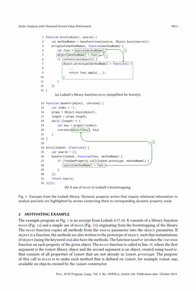
Fig. 1. Excerpts from the Lodash library. Dynamic property writes that require relational information toanalyze precisely are highlighted by arrows connecting them to corresponding dynamic property reads.
1○
2○
3○
2 MOTIVATING EXAMPLE
The example program in Fig. 1 is an excerpt from Lodash 4.17.10. It consists of a library functionmixin (Fig. 1a) and a simple use of mixin (Fig. 1b) originating from the bootstrapping of the library.The mixin function copies all methods from the source parameter into the object parameter. Ifobject is a function, the methods are also written to the prototype of object, such that instantiationsof object (using the keyword new) also have themethods. The function baseFor invokes the iterateefunction on each property of the given object. The mixin function is called in line 24, where the firstargument is the lodash library object and the second argument is an object, created using baseFor,that consists of all properties of lodash that are not already in lodash.prototype. The purposeof this call to mixin is to make each method that is defined on lodash, for example lodash.map,available on objects created by the lodash constructor.
Proc. ACM Program. Lang., Vol. 3, No. OOPSLA, Article 140. Publication date: October 2019.

140:4 Benno Stein, Benjamin Barslev Nielsen, Bor-Yuh Evan Chang, and Anders Mùller
This code contains three dynamic property read/write pairs ś indicated by the labels 1○, 2○, and3○ in Fig. 1 ś where relational information connecting the property name of the read and write isessential to avoid crippling loss of precision.
All three labelled read/write pairs are instances of a metaprogramming pattern called field copy
or transformation (FCT) [Ko et al. 2017, 2019], which consists of a property read operation x[a] anda property write operation y[b] = v where the property name b is a function of the property namea and the written value v is a function of the read value x[a]. This pattern is a generalization of thecorrelated read/write pattern [Sridharan et al. 2012], which requires that the property names arestrictly equal. Our technique attempts to generalize such syntactic patterns by identifying imprecisedynamic property writes semantically during the dataflow analysis. The benefits of this semanticapproach are twofold: it avoids the brittleness of syntactic patterns, and it only incurs additionalanalysis cost where needed, rather than at all locations matching a syntactic pattern.Analysis precision at dynamic property read and write operations is known to be critical for
static analysis for JavaScript programs [Andreasen and Mùller 2014; Ko et al. 2017, 2019; Sridharanet al. 2012]. If the abstract values of the property names are imprecise, then a naive analysis will mixtogether the values of the different properties, which often causes a catastrophic loss of precision.In the case of Lodash, such a naive analysis of the bootstrapping code would essentially cause allthe library functions to be mixed together, making it impossible to analyze any realistic applicationsof the library.
Existing attempts to address this problem are unfortunately insufficient. WALA [Sridharan et al.2012], SAFELSA [Park and Ryu 2015], and TAJS [Andreasen and Mùller 2014] use context-sensitivityand loop-unrolling to attempt to obtain precise information about the property names, but fail toprovide precise values of the variables methodName (at lines 4, 5, and 28) and key (at line 20).3
The CompAbs analyzer [Ko et al. 2017, 2019] takes a different approach that does not requireprecise tracking of the possible values of methodName and key. Instead, it attempts to syntacticallyidentify correlated dynamic property reads and writes and applies trace partitioning [Rival andMauborgne 2007] at the relevant property read operations. However, CompAbs fails to identify anyof the three highlighted read/write pairs in Fig. 1 due to the brittleness of syntactic patterns. Whileit might be possible to detect 2○ syntactically, the trace partitioning approach is insufficient forthat read/write pair, since the value in this case flows through a free variable (func) that is sharedacross all partitions. As a result, CompAbs fails to analyze the full Lodash library with sufficientprecision and ends up mixing together all properties of the lodash object.
Triggering Demand-Driven Value Refinement. Our approach is able to achieve sufficient precisionfor all three dynamic property read/write pairs in the example without relying on brittle syntacticpatterns to identify such pairs.The key idea underlying our technique is to detect semantically when an imprecise property
write is about to occur during the dataflow analysis, at which point we apply a targeted valuerefinement mechanism to recover the relational information needed to precisely determine whichvalues are written to which heap locations. More specifically, when the analysis encounters adynamic property write obj[p] = v and has imprecise abstract values for p and v, we decomposethe abstract value of v into a set of more precise partitions and then query the refinement mechanismto determine, for each partition, the possible values of p. Now, instead of writing the imprecise valueof v to all the property names of obj that match the imprecise value of p, we write each partition of v
3For example, achieving sufficient precision for methodName at lines 4 and 5 requires that the analysis can infer the preciselength and contents of the methodNames array, which is beyond the capabilities of those analyzers, even if using an (unsound)assumption that the order of the entries of the array returned by Object.keys is known statically.
Proc. ACM Program. Lang., Vol. 3, No. OOPSLA, Article 140. Publication date: October 2019.

Static Analysis with Demand-Driven Value Refinement 140:5
only to the corresponding refined property names of obj, thereby recovering relational informationbetween p and v.For example, suppose that the dataflow analysis reaches the dynamic property write of 3○
(at line 28) with an abstract state mapping the property name methodName to the abstract valuedenoting any string and the value func to the abstract value that abstracts all functions in lodash.We then decompose func into precise partitions ś one for each of the functions ś and query thevalue refinement mechanism for the corresponding sets of possible property names. Recoveringthat relational information, we obtain a unique function for each property name, such that thelodash.map function is assigned to source["map"], lodash.filter is assigned to source["filter"],etc., instead of mixing them all together. This technique handles case 1○ analogously, by detectingthe imprecision semantically at the dynamic property write.For property read/write pair 2○, however, the value to be written is a precise function (the
anonymous function in lines 7ś10) and the imprecise value func is a free variable declared in anenclosing function. In this case, value refinement is not triggered until func is called on line 9, atwhich point we apply the same value refinement technique as above and recover the necessaryrelational information to precisely resolve the target of that call, as described in further detail inSection 6.2.
Unlike abstraction-refinement techniques (see Section 8), this mechanism is able to recover rela-tional information and use it to regain precision in the dataflow analysis without any modificationsto its non-relational abstract domain and without restarting the entire analysis.
Value Refinement using Backwards Analysis. Our value refinement mechanism is powered by agoal-directed backwards abstract interpreter. Given a program location ℓ, a program variable y,and a constraint ϕ, it computes a bound on the possible values of y at ℓ in concrete states satisfyingϕ. We refer to the forward dataflow analysis as the base analysis and the backwards analysis as thevalue refiner.For example, if asked to refine the variable methodName at the location preceding line 28, under
the condition that func is the lodash.map function, our value refiner can determine that methodNamemust be "map". In doing so, the value refiner provides targeted information about the relationbetween func and methodName to the base analysis.Intuitively, the value refiner works by overapproximately traversing the abstract state space
backwards from the given program location, accumulating symbolic constraints about the pathsleading to that location. The traversal proceeds along each such path until a sufficiently precisevalue is obtained for the desired program variable. In this process, the value refiner takes advantageof the current call graph and the abstract states computed so far by the base analysis. The resultingabstract value thereby overapproximates the possible values of y at ℓ, for all program executionswhere ϕ is satisfied at ℓ and that are possible according to the call graph and abstract states fromthe base analysis. As we argue in Sections 4 and 7, the value refinement mechanism is sound eventhough it relies on information from the base analysis that has not yet reached its fixpoint.
3 A SIMPLE DYNAMIC LANGUAGE AND DATAFLOW ANALYSIS
To provide a foundation for explaining our demand-driven value refinement mechanism, in Sec-tion 3.1 we define the syntax and concrete semantics of a small dynamic language. This languageis designed for simplicity and clarity of presentation and is meant to illustrate some of the corechallenges in dynamic language analysis without the complexity that arises from a tested corecalculus for JavaScript such as λJS [Guha et al. 2010]. We then define our analysis over this minimallanguage in Section 3.2 and describe the extensions needed to handle the full JavaScript languagein Section 6.
Proc. ACM Program. Lang., Vol. 3, No. OOPSLA, Article 140. Publication date: October 2019.

140:6 Benno Stein, Benjamin Barslev Nielsen, Bor-Yuh Evan Chang, and Anders Mùller
variables x ,y, z ∈ Var
primitives p ∈ Prim ::= undef | true | false
| 0 | 1 | 2 | . . .
| "foo" | "bar" | . . .
statements s ∈ Stmt ::= x={} | x=y | x=p
| x=y ⊕ z | assume x
| x[y]=z | x=y[z]
operators ⊕ ::= + | − | = | , | . . .
locations ℓ ∈ Loc
control edges t ∈ Trans ::= ℓ →s ℓ′
Fig. 2. Concrete syntax for a simple dynamic language.
object addresses a ∈ Addr
memory addresses m ∈ Mem = Var ∪ (Addr × Prim)
values v ∈ Val = Addr ∪ Prim
states σ ∈ State = Mem → Val
[[·]] : Stmt → State → State
[[x={}]](σ ) = σ [x 7→ fresh(σ )]
[[x=y]](σ ) = σ [x 7→ σy]
[[x=p]](σ ) = σ [x 7→ p]
[[x=y ⊕ z]](σ ) = σ [x 7→ σy ⊕ σz]
[[assume x]](σ ) = σ if σx = true
[[x[y]=z]](σ ) = σ [(σx ,σy) 7→ σz] if σx ∈ Addrand σy ∈ Prim
[[x=y[z]]](σ ) = σ [x 7→ σ (σy,σz)]
Fig. 3. Denotational semantics and concrete domains.
3.1 A Simple Dynamic Language
The syntax and denotational semantics of our core dynamic language are shown in Fig. 2 and Fig. 3.A program in this language is an unstructured control-flow graph represented as a pair ⟨ℓ0,T ⟩ of
an initial location ℓ0 ∈ Loc and a set of control-flow edgesT ⊆ Trans. A program location ℓ ∈ Loc isa unique identifier. A memory addressm ∈ Mem is either a program variable x or an object property(a,p) where a is the address of an object and p is a primitive value. Concrete states σ ∈ State arepartial functions from memory addresses to values, which are either object addresses or primitives.We write ε for the empty state and use the notation σ [m 7→ v] to denote a state identical to σ
except at locationm where v is now stored, and σm to denote the value stored atm in σ or undef if
Proc. ACM Program. Lang., Vol. 3, No. OOPSLA, Article 140. Publication date: October 2019.
Static Analysis with Demand-Driven Value Refinement 140:7
a ∈�Addr , A ⊆ �Addr
p ∈�Prim =
⊥Prim
⊤Prim
· · · undef true 0 "foo" "bar" · · ·
m ∈�Mem = Var ∪ (�Addr × Prim)v ∈ Val = P(�Addr) ×�Prim
σ ∈�State = �Mem→ Val
L = Loc →�State
Fig. 4. Dataflow analysis lattice.
no such value exists. We also assume a helper function fresh(σ ) that returns an object address thatis fresh with respect to state σ .The denotation of a statement s is a partial function [[s]] from states to states. The collecting
semantics of a program ⟨ℓ0,T ⟩ is defined in terms of the denotational semantics as a function[[_]]⟨ℓ0,T ⟩ : Loc → P(State) that captures the reachable state space of the program, as the leastsolution to the following constraints:
ε ∈ [[ℓ0]]⟨ℓ0,T ⟩
∀σ ∈ [[ℓ]]⟨ℓ0,T ⟩ and ℓ →s ℓ′ ∈ T : [[s]](σ ) ∈ [[ℓ′]]⟨ℓ0,T ⟩
The first constraint says that the empty state ε is reachable at the initial location. The secondconstraint defines the successor states according to the denotational semantics.
3.2 Dataflow Analysis
We now describe a basic dataflow analysis for this minimal dynamic language, which we will extendin Section 4 with support for demand-driven value refinement.The analysis is expressed as a monotone framework [Kam and Ullman 1977] consisting of a
domain of abstract states and monotone transfer functions for the different kinds of statements.Programs can then be analyzed by a fixpoint solver computing an overapproximate abstract statefor each program location.4
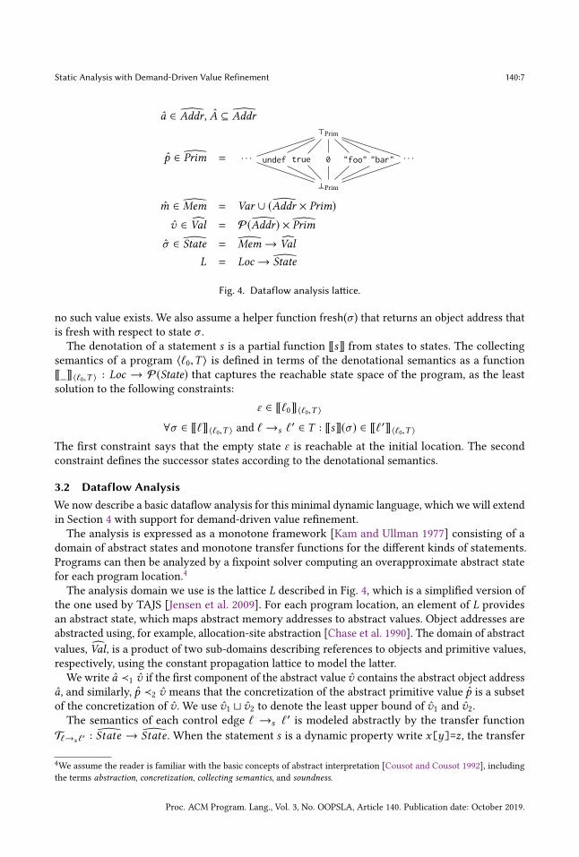
The analysis domain we use is the lattice L described in Fig. 4, which is a simplified version ofthe one used by TAJS [Jensen et al. 2009]. For each program location, an element of L providesan abstract state, which maps abstract memory addresses to abstract values. Object addresses areabstracted using, for example, allocation-site abstraction [Chase et al. 1990]. The domain of abstract
values, Val, is a product of two sub-domains describing references to objects and primitive values,respectively, using the constant propagation lattice to model the latter.
We write a ≺1 v if the first component of the abstract value v contains the abstract object addressa, and similarly, p ≺2 v means that the concretization of the abstract primitive value p is a subsetof the concretization of v . We use v1 ⊔ v2 to denote the least upper bound of v1 and v2.The semantics of each control edge ℓ →s ℓ
′ is modeled abstractly by the transfer functionTℓ→s ℓ
′ : �State → �State . When the statement s is a dynamic property write x[y]=z, the transfer
4We assume the reader is familiar with the basic concepts of abstract interpretation [Cousot and Cousot 1992], includingthe terms abstraction, concretization, collecting semantics, and soundness.
Proc. ACM Program. Lang., Vol. 3, No. OOPSLA, Article 140. Publication date: October 2019.

140:8 Benno Stein, Benjamin Barslev Nielsen, Bor-Yuh Evan Chang, and Anders Mùller
ℓ1 ℓ2 ℓ3
t = x[p] y[p] = t
Fig. 5. A program fragment with a correlated property read/write pair.
function is defined as follows:
Tℓ→s ℓ′(σ )(m) =
{σm ⊔ σz if m = (a,p) ∧ a ≺1 σx ∧ p ≺2 σy
σm otherwise
In other words, the analysis models such an operation by weakly5 updating all the affected abstractmemory addresses with the abstract value of z. Due to the limited space, we omit descriptions ofthe remaining analysis transfer functions for other kinds of statements; it suffices to require thatthey soundly overapproximate the semantics [Cousot and Cousot 1977].The refinement mechanism directly involves the fixpoint solver. As customary in dataflow
analysis, we assume the fixpoint solver uses a worklist algorithm to determine which locations toprocess next each time a transfer function has been applied [Kildall 1973]. A worklist algorithmrelies on a map dep : Loc → P(Loc), such that dep(ℓ) contains all direct dependents of ℓ, in ourcase the successors {ℓ′ | ℓ →s ℓ
′ ∈ Trans}. For a worklist algorithm to be sound, it must add all thelocations dep(ℓ) to the worklist when the abstract state at ℓ is updated.
Example. Fig. 5 shows a program fragment with a correlated property read/write pair likein Section 2. Assume σ is an abstract state where x and y point to distinct objects (ax and ay,respectively), p is any primitive value, the x object has three properties (named "a", "b", and "c")with different values, and the y object is empty:
σx = ({ax},⊥Prim)
σy = ({ay},⊥Prim)
σp = (∅,⊤Prim)
σ (ax, "a") = ({axa},⊥Prim)
σ (ax, "b") = ({axb},⊥Prim)
σ (ax, "c") = (∅,⊤Prim)
σ (ay,p) = (∅,⊥Prim) for all p ∈ Prim
The transfer function for t = x[p] with this abstract state at initial program location ℓ1 yieldsan abstract state at ℓ2 that maps t to ({axa, axb},⊤Prim). Next, the transfer function for y[p] = t asdefined above results in an abstract state at ℓ3 where every property of the abstract object ay hasthe same abstract value as t, meaning that they all may point to any of the two abstract objects axaand axb and have any primitive value. Consequently, the analysis result is very imprecise. In thefollowing section, we explain how the basic dataflow analysis can be extended with demand-drivenvalue refinement to avoid the precision loss.
4 DEMAND-DRIVEN VALUE REFINEMENT
In this section, we introduce the notion of a value refiner (Section 4.1), discuss when and how toapply value refinement during the base analysis (Section 4.2), and explain how to integrate a valuerefiner into the base analysis in a way that allows the value refiner to benefit from the abstractstates that are constructed by the base analysis (Section 4.3).
5Our implementation for JavaScript uses a more expressive heap abstraction that permits strong updates [Chase et al. 1990;Jensen et al. 2009] in certain situations.
Proc. ACM Program. Lang., Vol. 3, No. OOPSLA, Article 140. Publication date: October 2019.

Static Analysis with Demand-Driven Value Refinement 140:9
4.1 Value Refinement
A value refiner is a function
R : Loc × Var × Constraint → P(Val)
that, given a program location ℓ ∈ Loc, a program variable y ∈ Var , and a constraint ϕ ∈
Constraint = Var × Val yields a set of abstract values that are possible for y at ℓ in states that satisfyϕ. We refer to an invocation of the value refiner function by the base analysis as a refinement query.For the refinement queries we need, a constraint is simply a pair of a program variable and anabstract value, written z 7→ v , specifying that the variable z has value v .We require R to be sound in the sense that it overapproximates all possible behaviors of the
program according to the collecting semantics: for every state σ ∈ [[ℓ]]⟨ℓ0,T ⟩ where ℓ is a locationin the program ⟨ℓ0,T ⟩ and the abstraction of σ satisfies the constraint ϕ, the value σy is in theconcretization of an abstract value in R(ℓ,y,ϕ) for any y.
In Section 5 we present a specific value refiner; for the remainder of the current section we canthink of the value refiner as a black-box component with the above properties.
4.2 Using Value Refinement in Dataflow Analysis
Value refinement can in principle be invoked whenever the base analysis detects that a potentiallycritical loss of precision is about to happen, to provide more precise abstract values. As discussedin Section 2, such precision losses often occur in connection with dynamic property writes, so wehere focus on that kind of operation. In Section 6.2, we consider value refinement also at variableread operations.
First, we define a helper function Part : Val → P(Val) that partitions an abstract value into a setof abstract values, each containing at most one abstract memory address:
Part(A, p) ={ ({a},⊥Prim) | a ∈ A } ∪
{{(∅, p)} if p , ⊥Prim∅ otherwise
Continuing the example from Section 3.2, we have:
Part({axa, axb},⊤Prim) = {({axa},⊥Prim), ({axb},⊥Prim), (∅,⊤Prim)}
We now incorporate value refinement into the base analysis by replacing the ordinary transferfunction Tℓ→s ℓ
′ from Section 3.2 by a new transfer function T VRℓ→s ℓ
′ . The domain of the baseanalysis remains unchanged (unlike traditional abstraction refinement techniques). The new transferfunction is defined as follows when s is a dynamic property write statement x[y]=z:
T VRℓ→s ℓ
′(σ )(m) =
σm ⊔ V (σ , ℓ,y, z,p) if ⊤Prim ≺2 σy ∧ |Part(σz)| > 1∧ m = (a,p) ∧ a ≺1 σx
Tℓ→s ℓ′(σ )(m) otherwise
where the abstract value being written is
V (σ , ℓ,y, z,p) =⊔ {
z ∈ Part(σz)�� ∃y ∈ R(ℓ,y, z 7→ z) : p ≺2 y
}
This modified transfer function captures some of the key ideas of our approach, so we carefullyexplain each part of the definition. The first case of the transfer function definition shows when andhow value refinement is used, and the second case simply falls back to the ordinary transfer function.Value refinement is applied when the analysis has an imprecise value fory (i.e.,⊤Prim ≺2 σy) and animprecise value for z that is partitioned nontrivially (i.e., |Part(σz)| > 1), provided that the desiredabstract memory address m denotes an object property (i.e., m = (a,p) for some abstract object
Proc. ACM Program. Lang., Vol. 3, No. OOPSLA, Article 140. Publication date: October 2019.

140:10 Benno Stein, Benjamin Barslev Nielsen, Bor-Yuh Evan Chang, and Anders Mùller
address a and property name p). The abstract value V (σ , ℓ,y, z,p) being written is then computedby issuing a refinement query R(ℓ,y, z 7→ z) for each partition z of σz (i.e., z ∈ Part(σz)). Each ofthe resulting abstract values y describes a possible value of y under the constraint that z has valuez. In this way, rather than writing the imprecise abstract value σz to all properties of a, the analysiswrites each of the more precise abstract values z to the corresponding refined property name pthat matches y (i.e., p ≺2 y).
Example. Recall that in the example from Section 3.2, at the dynamic property write y[p] = t
the base analysis has imprecise abstract values for the property name p and for the value t beingwritten. More specifically, Part partitions the latter into three more precise abstract values as shownabove. This means that the condition is satisfied for using value refinement, so the modified transferfunction then issues three refinement queries. Using the value refiner that we present in Section 5yields the following results:
R(ℓ2, p, t 7→ ({axa},⊥Prim)) = {(∅, "a")}
R(ℓ2, p, t 7→ ({axb},⊥Prim)) = {(∅, "b")}
R(ℓ2, p, t 7→ (∅,⊤Prim)) = {(∅, "c")}
The transfer function then writes each refined abstract value only to the relevant property of ay,instead of mixing them all together like the ordinary transfer function. For example, the resultingstate maps (ay, "a") to ({axa},⊥Prim). The base analysis then proceeds with this more preciseabstract state.Notice that the base analysis has only one abstract value per abstract memory address and
program location, whereas the value refiner returns a set of abstract values at each refinementquery. In the example described above, each of the refinement query results contains only oneabstract value, but when applying our technique to the examples from Section 2, we benefit fromthe possibility that R can return multiple abstract values: Some methods of the lodash object areaccessible via multiple names, for example lodash.entries and lodash.toPairs are aliases. In thiscase, querying the value refiner for the possible property names given that the value being writtenis that specific function, the result can be expressed as the set of the two strings "entries" and"toPairs" instead of the less precise single abstract value representing all possible strings.
4.3 Using the Base Analysis During Refinements
The value refiner can leverage the base analysis state to allow for more efficient implementation. Forthe dataflow analysis defined in Section 3.2, the refiner can read partially-computed abstract states;in our JavaScript implementation (see Section 6.1), the refiner also uses the partially-computed callgraph.We argue that this is sound even though the base analysis has not yet reached a fixpoint whenthe refiner is invoked. This extended kind of a value refiner is denoted RX where X : Loc →�Stateis a lattice element of the base analysis.For the example from Section 3.2, RX can obtain the value of the variable x at ℓ1 simply by
looking up X (ℓ1)(x) from the base analysis, without needing to traverse all the way back to wherethe value of x was created. Similarly, for analysis of JavaScript, using the call graph available fromthe base analysis allows the value refiner to narrow its exploration when stepping from functionentry points to call sites.For this mechanism to retain analysis soundness, we slightly modify the base analysis. Recall
from Section 3.2 that the base analysis relies on a worklist of program locations. Now, whenever arefinement query is triggered by the base analysis at some program location ℓ and the value refinerreads from the abstract state X (ℓ′), we extend the dep map to record that ℓ depends on ℓ′. In this
Proc. ACM Program. Lang., Vol. 3, No. OOPSLA, Article 140. Publication date: October 2019.

Static Analysis with Demand-Driven Value Refinement 140:11
symbolic variables x, y, z, res ∈ Var
symbolic expressions e ∈�Expr ::= x | v | e1 ⊕ e2
symbolic stores φ ∈�Store ::= h ∧ π | φ1 ∨ φ2
heap constraints h ::= true | unalloc(x ) | x 7→ x | x1[x2] 7→ x3 | h1 ∗ h2
pure constraints π ::= true | e | π1 ∧ π2
valuations η ∈ Valua : Var → Val
(a) Abstractions for value refinement. Recall from Section 3 that ⊕ ranges over binary operators, x overprogram variables, and v over abstract values.
eval : (�Expr × Valua) → P(Val)eval(x, η) = {ηx }
eval(v, η) = γval(v)
eval(e1 ⊕ e2, η) =
{v1 ⊕ v2
����v1 ∈ eval(e1, η)
∧ v2 ∈ eval(e2, η)
}
(b) Abstract expression evaluation function eval. The notation γval(v) refers to the concretization of v .
γ (h ∧ π ) = γ (h) ∩ γ (π )
γ (φ1 ∨ φ2) = γ (φ1) ∪ γ (φ2)
γ (true) = State × Valua
γ (e) =
{(σ , η)
�� true ∈ eval(e, η)}
γ (π1 ∧ π2) = γ (π1) ∩ γ (π2)
γ (unalloc(x )) =
{(σ , η)
�� ∀v : σ (η(x ), v) = undef}
γ (x 7→ x ) =
{(σ , η)
�� σx = η(x )}
γ (x1[x2] 7→ x3) =
{(σ , η)
�� σ (η(x1), η(x2)) = η(x3)}
γ (h1 ∗ h2) =
{(σ1 ⊎ σ2, η)
����(σ1, η) ∈ γ (h1) ∧ (σ2, η) ∈ γ (h2)
∧ dom(σ1) ∩ dom(σ2) = ∅
}
(c) Concretizations γ for symbolic stores φ, heap constraints h, and pure constraints π . We denote by ⊎ theunion of two partial functions with disjoint domains.
Fig. 6. Syntax and concretizations of abstractions used for value refinement.
way, if the abstract state at ℓ′ changes later during the base analysis, the result of the invocation ofthe value refiner is invalidated and eventually recomputed.6
As such, the soundness criterion from Section 4.1 for the value refiner needs to be adjusted byweakening the soundness requirement so that the value refiner needs only overapproximate thoseconcrete program behaviors that are abstracted by the current base analysis state. We say thata trace ℓ0 →s1 ℓ1 →s2 · · · →sn ℓn is abstracted by a base analysis state X ∈ L if, for all k ≤ n,([[sk ]] ◦ [[sk−1]] ◦ · · · ◦ [[s1]])(ε) is in the concretization of X (ℓk ). Then, a refiner RX is sound if σy isin the concretization of an abstract value in RX (ℓ,y,ϕ) for every concrete state σ ∈ [[ℓ]]⟨ℓ0,T ⟩ thatsatisfies ϕ and is the final state of a trace that is abstracted by X and ends at ℓ.
6To improve performance, our implementation actually tracks these extra dependencies in a more fine-grained manner, asdescribed in Section 6.3.
Proc. ACM Program. Lang., Vol. 3, No. OOPSLA, Article 140. Publication date: October 2019.

140:12 Benno Stein, Benjamin Barslev Nielsen, Bor-Yuh Evan Chang, and Anders Mùller
Conseqence
φ ′2 ⇒ φ2 ⟨φ ′2⟩ s ⟨φ′1⟩ φ1 ⇒ φ ′1
⟨φ2⟩ s ⟨φ1⟩
Frame
⟨h′1 ∧ π′⟩ s ⟨h1 ∧ π ⟩ mod(s) ∩ fv(h2) = ∅
⟨h′1 ∗ h2 ∧ π′⟩s⟨h1 ∗ h2 ∧ π
⟩
Disjunction
⟨φ ′l ⟩ s ⟨φl ⟩ ⟨φ ′r ⟩ s ⟨φr ⟩⟨φ ′l ∨ φ
′r
⟩s⟨φl ∨ φr
⟩
BinOp
h = y 7→ y ∗ z 7→ z⟨h ∧ π ∧ x = y ⊕ z
⟩
x = y ⊕ z⟨h ∗ x 7→ x ∧ π
⟩
NewObj
⟨unalloc(x) ∧ π ∧
(∧i zi = undef
)⟩
x = {}⟨x 7→ x ∗
(∗i x[_] 7→ zi
)∧ π
⟩
Alias
⟨(y 7→ y ∧ π )[y/x]
⟩
x = y⟨x 7→ x ∗ y 7→ y ∧ π
⟩
ReadProp
h = y 7→ y ∗ z 7→ z ∗ y[z] 7→ x ′
⟨(h ∧ π )[x ′/x]
⟩
x = y[z]⟨h ∗ x 7→ x ∧ π
⟩
Assume
h = x 7→ x⟨h ∧ x ∧ π
⟩assume x
⟨h ∧ π
⟩
WriteProp
h = x 7→ x ∗ y 7→ y ∗ z 7→ z⟨(h ∧ π )[z/z ′]
⟩x[y] = z
⟨h ∗ x[y] 7→ z ′ ∧ π
⟩
Constant
⟨true ∧ π ∧ x = p
⟩x = p
⟨x 7→ x ∧ π
⟩
Fig. 7. Rules for refutation-sound backwards abstract interpretation. We denote the set of memory locations
possibly modified by a statement s by mod(s), the free variables of a heap constraint h by fv(h), and thesubstitution of symbolic variable x for y in a symbolic store φ by φ[x/y]. To simplify the presentation, withoutloss of generality, we assume the program has been normalized so that any statement involving multipleprogram variables uses distinct variables.
Soundness. Since we require that the refiner RX is sound with respect to those traces abstractedby the base analysis state, T VR
ℓ→s ℓ′ is sound when that base analysis state abstracts the full concrete
semantics, which is guaranteed at a fixpoint. If the base analysis state does not yet abstract the fullconcrete collecting semantics, then RX ’s refinements are only sound so long as the information theyread from the base analysis state is unchanged. However, by adding additional dependency edgeswherever such a read occurs, we ensure that any refinement query that used stale information willbe invalidated and recomputed. We refer to Appendix A for a more detailed discussion.
5 BACKWARDS ABSTRACT INTERPRETATION FOR VALUE REFINEMENT
In this section, we define a sound value refiner R← based on goal-directed backwards abstractinterpretation. The value refiner R← works by exploring backwards from the abstract state whereit was triggered, overapproximating the set of states from which that state is reachable using anabstract domain based on separation logic constraints. We also detail the construction of a refinerR←X that extends R← to access base analysis abstract state during value refinement.
This value refiner is goal-directed in the sense that it only traverses the subset of the control-flowgraph relevant to a given refinement query and only computes transfer functions that directlyaffect its constraints. As such, it is quite precise with respect to a fixed property of interest withoutincurring the cost of applying that same precision to the full program.
Proc. ACM Program. Lang., Vol. 3, No. OOPSLA, Article 140. Publication date: October 2019.

Static Analysis with Demand-Driven Value Refinement 140:13
5.1 Abstract Domain
The abstract domain of R← is a constraint language over memory states. The syntax and semanticsof this constraint language are given in Fig. 6. A symbolic store φ is a disjunctive normal formexpression over heap constraints h and pure constraints π . Each clause represents a symbolic store,while the top-level disjunction permits case-splitting.
Heap constraints h are defined using an intuitionistic separation logic [Ishtiaq and O’Hearn 2001]wherein a single-cell heap constraint (i.e., x 7→ x or x1[x2] 7→ x3) holds for any heap containingthat cell, not just for those heaps comprised only of that single cell. This results in a monotoniclogic in which heap constraints h are preserved under heap extension. That is, if an intuitionisticseparation logic assertion h holds for some concrete state σ , then h must also hold for all extensionsσ ′ of σ . This succinctly supports a goal-directed analysis, in which we want to infer informationonly about some sub-portion of the heap.
Pure constraints π are either symbolic expressions e or conjunctions thereof; the pure constrainte holds whenever it could possibly evaluate to true according to the abstract expression evaluationfunction eval. By defining pure constraints over abstract values v rather than concrete values v , wewill be able to seamlessly integrate information from the abstract state of the base analysis duringrefinement, as discussed in Section 4.3.
We denote byφ∧φ ′ conjunction and re-normalization to DNF after alpha-renaming free symbolicvariables in φ ′ such that all memory addresses are mapped to the same symbolic variable by bothsymbolic stores. For example, (x 7→ x ∧ x > 0)∧(x 7→ y∧y < 5) reduces to x 7→ x ∧(x > 0∧ x < 5).
5.2 Backwards Abstract Interpretation
We define the analysis in terms of refutation sound [Blackshear et al. 2013] Hoare triples of theform ⟨φ⟩ s ⟨φ ′⟩, which are given in Fig. 7.Refutation soundness is similar to the standard definition of soundness for Hoare logic (i.e.,
partial correctness), but in the opposite direction: a triple is refutation sound if and only if((σ ′,η) ∈ γ (φ ′) ∧ [[s]](σ ) = σ ′) ⇒ (σ ,η) ∈ γ (φ) holds for all σ , σ ′, and η. That is, a triple is refuta-tion sound if any concrete run through s ending in a state satisfying the postcondition φ ′ musthave started in a state satisfying the precondition φ.
These triples are best read from postcondition to precondition, since that is the natural directionin which to understand refutation soundness and the direction in which the analysis actuallyapplies them.The first three rules in Fig. 7 are integral structural components of the system that are not
specific to any particular statement form. The Conseqence rule allows the analysis to strengthenpreconditions and weaken postconditions, making explicit our notion of refutation soundness andallowing other rules to materialize heap cells as needed; Frame enables local heap reasoning; andDisjunction splits reasoning over each disjunct of a symbolic store.
The remaining rules abstract the concrete semantics of their respective statement forms. Read-Prop, WriteProp, and Alias transfer any postcondition constraints on their left-hand-side toprecondition constraints on their right-hand-side; NewObj constrains any properties of the al-located object to be undef and asserts that the object is now unallocated, which ensures (byseparation) that no such properties can be framed out by Frame; BinOp and Constant use pureequality constraints to precisely model the concrete semantics; and Assume directly encodes theassumption into a pure constraint.
Our value refiner R← : Loc × Var × Constraint → P(Val) is based on backwards abstractinterpretation using the judgment ⟨φ⟩ s ⟨φ ′⟩. We introduce a distinguished symbolic variable resto represent the value that is being refined as we move backwards through the program. Note that
Proc. ACM Program. Lang., Vol. 3, No. OOPSLA, Article 140. Publication date: October 2019.

140:14 Benno Stein, Benjamin Barslev Nielsen, Bor-Yuh Evan Chang, and Anders Mùller
R← is implicitly parameterized by a specific program ⟨ℓ0,T ⟩, but does not have access to abstractstates from the base analysis as discussed in Section 4.3; integration with the base analysis will bedetailed in Section 5.3.Given a refinement query R←(ℓ,x ,y 7→ v), we first encode the inputs as a symbolic store
x 7→ res ∗ y 7→ y ∧ y = v . Then, we algorithmically apply the Hoare triples from Fig. 7 backwardsfrom ℓ in T to compute a symbolic store for each backwards-reachable location, using a standardworklist algorithm to ensure correctness and minimize redundant work and applying the wideningtechnique of Blackshear et al. [2013] to compute fixpoints over loops.Due to refutation soundness, it is sound for the backwards abstract interpreter to stop at any
point. Since each successive application of a rule from Fig. 7 computes an abstract preconditionthat a concrete execution must satisfy to reach the given abstract postcondition, the constraints onres grow more precise the more of the program is analyzed but are overapproximate every step ofthe way. As such, the stopping criterion of R← can be tuned, offering a tradeoff between refinementprecision and performance. In our implementation for JavaScript, we stop the backwards traversalalong a path if sufficient precision has been reached for the refinement variable res, meaning thatits abstract value is either a singleton set of object addresses or a non-⊤Prim abstract primitive.This analysis continues either until we reach a least fixpoint in the symbolic store domain
(partially ordered under implication) or the stopping criterion is fulfilled for all symbolic storesin the worklist. At that point, we compute an upper bound on the value of res in all remainingsymbolic stores and return the corresponding set of abstract values.
Example. Recall that the base analysis issues three refinement queries for the example fromSection 4.2, the first one being R←(ℓ2, p, t 7→ ({axa},⊥Prim)). This query is encoded as the initialsymbolic store p 7→ res ∗ t 7→ t ∧ t = ({axa},⊥Prim) at the program location ℓ2. From there, R←
uses the Conseqence and ReadProp rules from Fig. 7 to construct the triple
⟨p 7→ res ∗ x 7→ x ∗ x[res] 7→ t ∧ t = ({axa},⊥Prim)
⟩
t = x[p]⟨p 7→ res ∗ t 7→ t ∧ t = ({axa},⊥Prim)
⟩
which precisely models the dynamic property read t= x[p] and yields a precondition symbolicstore expressing a refinement of the value of p when x[p] has value ({axa},⊥Prim). We continue thisexample in the following section to show how the value refiner reaches the final result {(∅, "a")}.
Soundness. By refutation soundness, applying the Hoare rules from Fig. 7 backwards soundlyoverapproximates the states from which the refinement location is reachable. By exhaustivelytracking the value of res on all backward abstract paths from the refinement location, R← thereforecomputes an overapproximation of the variable being refined with respect to the concrete collectingsemantics. We refer to Appendix B for a proof sketch.
5.3 Integration of Base Analysis State
We now extend R← to leverage abstract state from the base analysis as described in Section 4.3,thereby constructing a value refiner R←X that is parameterized by a base analysis abstract state X .In particular, we describe a procedure by which a symbolic store φ and base analysis state X can becombined to compute a refinement that the symbolic store φ is not able to on its own. Essentially,when R←X has a symbolic store φ refining a property’s name under a constraint on that property’svalue, it accesses the base analysis state to determine possible property names satisfying thoseconstraints and then returns that set. We refer to this procedure as property name inference.
Proc. ACM Program. Lang., Vol. 3, No. OOPSLA, Article 140. Publication date: October 2019.

Static Analysis with Demand-Driven Value Refinement 140:15
In more detail, this mechanism works as follows. If, during the backwards abstract interpretationas described for R← in the previous section, the current symbolic store φ matches
x 7→ x ∗ x[res] 7→ y ∗ h ∧ y = v ∧ π
for some x , x , y, v , undef, h, and π , then property name inference is applied. Intuitively, thiscondition means that the abstract value of the res property of x is v , which allows R←X to determinethe desired set of property names by reading the base analysis state at that location. We define afunction infer-prop-names to compute that refinement:
infer-prop-names(φ, σ ) =
{p
����∃a : a ≺1 σx ∧ (a,p) ∈ dom(σ )∧ σ (a,p) ⊓ v , (∅,⊥Pr im)
}
Intuitively, infer-prop-names checks each property (a,p) on the object x , returning the names p ofthose properties whose abstract value intersects with v .The property name inference mechanism thus refines the abstract names of object properties.
Our implementation uses the same idea to also refine abstract values of properties, which we returnto in Section 6.2.
Example. Continuing the example from Section 5.2, φ is of the form specified above, so theanalysis applies property name inference to compute a refinement for p. Computing the refinementinfer-prop-names(φ,X (ℓ1)) gives the names of those properties in X (ℓ1) that satisfy φ, meaningthat the property value intersects with ({axa},⊥Prim). In this case, "a" is the only such propertyname according to the value of X (ℓ1) given in Section 3.2, so the refiner returns {(∅, "a")}. In thissimple example, a single step backwards suffices before the stopping criterion is fulfilled, due tothe integration of the base analysis state, but multiple steps are often needed in practice.
6 INSTANTIATION FOR JAVASCRIPT
Our implementation, TAJSVR,7 generalizes to JavaScript the ideas presented in the previous sectionsfor the simple dynamic language. As base dataflow analysis TAJSVR uses the existing tool TAJS,extended as explained in Section 4.3. The other main component of the implementation is the valuerefiner, built from scratch and based on the design given in Section 5. The two components areimplemented separately ś the base analysis in Java (approximately 2500 lines of code on top ofTAJS) and the refiner in Scala (approximately 2400 lines of code) ś and communicate only througha minimal interface that allows the base analysis to issue refinement queries and the refiner to readpartially-computed base analysis state, request control-flow information to traverse the program, orperform property name inference as described in Section 5.3. The implementation and experimentaldata are available at https://www.brics.dk/TAJS/VR.
6.1 A Value Refiner for JavaScript
Many JavaScript language features that are not directly in the minimal dynamic language arestraightforward to handle. However, for-in loops, interprocedural control flow, and prototype-based inheritance are nontrivial and require some additional machinery in the backwards analysis.
for-in loops. In order to handle for-in loops efficiently, the refiner analyzes the loop body undercontexts corresponding to the properties of the loop object in the base analysis state.
That is, upon reaching the exit of a for-in loop, the value refiner queries the base analysis statefor a set of property names on the loop object, generating one context for each of them and oneadditional context as a catch-all for all other property names. Then, it analyzes the loop body onceper context before joining the results and continuing backwards from the loop entry.
7TAJS with demand-driven Value Refinement
Proc. ACM Program. Lang., Vol. 3, No. OOPSLA, Article 140. Publication date: October 2019.

140:16 Benno Stein, Benjamin Barslev Nielsen, Bor-Yuh Evan Chang, and Anders Mùller
Interprocedural control flow. In order to soundly navigate interprocedural control flow in thevalue refinement analysis, we rely on the partially-computed call graph from the base analysiswhile maintaining a stack of return targets where possible. That is, when reaching a call site,the analysis pushes that location (along with any locally-scoped constraints) onto a stack beforejumping to the exit of all possible callees in the base analysis call graph. Then, upon reaching afunction entry point, it pops a stack element and jumps to the corresponding call site or, if the stackis empty, jumps to all callers of the current function in the base analysis call graph. When usingan unbounded stack, it analyzes function calls fully context-sensitively and therefore relies on atimeout to ensure termination, but k-limiting the stack height would ensure termination (withouta timeout) while analyzing function calls with k-callstring context sensitivity.
Prototype-based inheritance. Handling prototype-based inheritance is more complicated since thesemantics of a dynamic property access depend not only on the values of the object and propertyname but also on the prototype relations and properties of other objects in the program.Our implementation reasons about prototype-based inheritance by introducing łprototype
constraintsž at property reads to keep track of prototype relationships between relevant symbolicvariables. These constraints are manipulated as the analysis evaluates other property writes andmodifications to the prototype graph; for example, when encountering a property write under aprototype constraint, the analysis splits into a disjunction on whether or not the write is to thememory location whose read produced the prototype constraint. This allows the analysis to reasonabout prototype semantics, even in programs that dynamically modify the prototype graph.
6.2 Functions with Free Variables
As mentioned in Section 2, the dynamic property read/write pair 2○ in the example in Fig. 1adiffers from 1○ and 3○, because the values flow from the property read to the associated write via afree variable that is declared in an enclosing function. It is critical that the analysis does not mixtogether the different functions of the source object. For example, in clients of Lodash, the functionvalue lodash([1, 2]).map is the one created in line 7 where methodName is "map". If the programcontains a call to that function, then at the call func.apply(...) in line 9, the analysis must haveenough precision to know that func is the same function as source["map"].We achieve that degree of precision by adjusting the base analysis as follows. At the dynamic
property write in line 7, the analysis detects that in the current abstract state, the property name(i.e. methodName) is imprecise and that the value being written denotes a function that contains afree variable with an imprecise value as noted in Section 2. The analysis then annotates the abstractvalue being written with the memory address of methodName and the current program location ℓ7for later use. Every property of object.prototype then has this single annotated abstract value.When the analysis later encounters a property read operation that yields such an annotated
value, the value is modified to reflect the property name, which can now be resolved. For example,at an expression lodash([1, 2]).map, the resulting abstract value describes a function that hasbeen created at a point where the value of methodName was "map".If that function is called, the analysis reaches line 9 and then issues the refinement query
R←X (ℓ7, func, methodName 7→ "map") to learn the possible values of func at line 7 under the constraintthat methodName has the value "map". When the value refiner reaches the dynamic property read inline 4 during the backwards analysis, it can use the base analysis state to read source["map"] (ashinted in Section 5.3), which provides the desired precise value for func.Note that with this mechanism, our base analysis does not only trigger refinement at dynamic
property writes as described in Section 4.2, but also for variable reads of imprecise free variables asdescribed above.
Proc. ACM Program. Lang., Vol. 3, No. OOPSLA, Article 140. Publication date: October 2019.

Static Analysis with Demand-Driven Value Refinement 140:17
6.3 Performance Improvements
Recall from Section 4.3 that a location ℓ is added to the worklist when a refinement query at ℓhas accessed the abstract state X (ℓ′) and that abstract state has changed. Our implementationuses a more fine-grained notion of dependencies by keeping track of the individual dataflow factsinstead of entire abstract states, such that ℓ is only added to the worklist when the state change atℓ′ invalidates the dataflow facts that were previously accessed from ℓ′.Additionally, our implementation caches refinement query results, exploiting the fact that the
result of a query RX (ℓ,y,ϕ) depends only on the three parameters and the dataflow facts in X thatare accessed by the value refiner.
7 EVALUATION
We evaluate the demand-driven value refinement technique by considering the following researchquestion:
Can TAJSVR analyze programs that other state-of-the-art tools are unable to analyzesoundly and with high precision?
To provide insights into why the mechanism is effective when analyzing real-world programs, wealso investigate how many value refinement queries are issued, how often the value refiner is ableto produce more precise results than the base analysis, and how much analysis time is typicallyspent on value refinement.
7.1 Comparison with State-of-the-Art Analyzers
We compare TAJSVR with two existing state-of-the-art analysis tools: TAJS [Andreasen and Mùller2014; Jensen et al. 2009] and CompAbs [Ko et al. 2017, 2019]. TAJS is the base dataflow analysis uponwhich TAJSVR is built; it is designed for JavaScript type analysis but performs no value refinement.CompAbs ś described in further detail in Sections 2 and 8 ś is a tool built on top of SAFE [Lee et al.2012] that attempts to syntactically identify problematic dynamic property access patterns andapplies trace partitioning at those locations.We evaluate each tool on three sets of benchmarks: a series of micro-benchmarks designed
as minimal representative examples of dynamic property manipulation patterns, a collection ofevaluation suites drawn from other JavaScript static analysis research papers, and the unit test suitesof two popular JavaScript libraries that are unanalyzable by the existing static analysis tools. Allexperiments have been performed on an Ubuntu machine with 2.6 GHz Intel Xeon E5-2697A CPUrunning a JVM with 10 GB RAM. Collectively, the results indicate that the relational informationprovided by value refinement is critical for the analysis of challenging JavaScript programs.
Micro-Benchmarks. Following the approach of Ko et al. [2017], we first evaluate TAJSVR on aseries of small benchmarks containing dynamic property access patterns known to be difficult forstatic analysis. Source code for these benchmarks can be found in Ko et al. [2017] (CF, CG, AF, andAG) or at https://www.brics.dk/TAJS/VR (M1, M2, and M3).
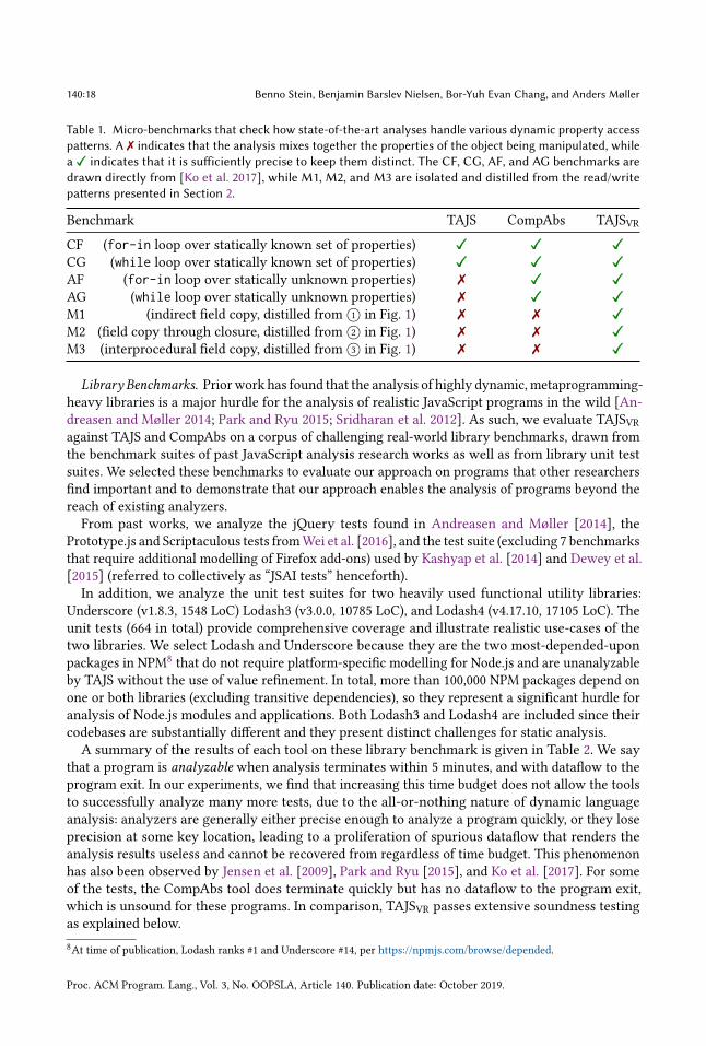
The results, shown in Table 1, are as expected: TAJS only handles the benchmarks CF andCG where the property names are known statically, and CompAbs fails to successfully analyzeany of M1, M2 or M3: M1 and M3 because the relevant read/write pair is not detected by thesyntactic patterns, and M2 because the trace partitioning mechanism does not distinguish closureson free variables within the partitions. TAJSVR handles all seven programs precisely by the use ofdemand-driven value refinement.
Proc. ACM Program. Lang., Vol. 3, No. OOPSLA, Article 140. Publication date: October 2019.
140:18 Benno Stein, Benjamin Barslev Nielsen, Bor-Yuh Evan Chang, and Anders Mùller
Table 1. Micro-benchmarks that check how state-of-the-art analyses handle various dynamic property accesspatterns. A ✗ indicates that the analysis mixes together the properties of the object being manipulated, whilea ✓✓✓ indicates that it is sufficiently precise to keep them distinct. The CF, CG, AF, and AG benchmarks aredrawn directly from [Ko et al. 2017], while M1, M2, and M3 are isolated and distilled from the read/writepatterns presented in Section 2.
Benchmark TAJS CompAbs TAJSVR
CF (for-in loop over statically known set of properties) ✓✓✓ ✓✓✓ ✓✓✓
CG (while loop over statically known set of properties) ✓✓✓ ✓✓✓ ✓✓✓
AF (for-in loop over statically unknown properties) ✗ ✓✓✓ ✓✓✓
AG (while loop over statically unknown properties) ✗ ✓✓✓ ✓✓✓
M1 (indirect field copy, distilled from 1○ in Fig. 1) ✗ ✗ ✓✓✓
M2 (field copy through closure, distilled from 2○ in Fig. 1) ✗ ✗ ✓✓✓
M3 (interprocedural field copy, distilled from 3○ in Fig. 1) ✗ ✗ ✓✓✓
Library Benchmarks. Priorwork has found that the analysis of highly dynamic, metaprogramming-heavy libraries is a major hurdle for the analysis of realistic JavaScript programs in the wild [An-dreasen and Mùller 2014; Park and Ryu 2015; Sridharan et al. 2012]. As such, we evaluate TAJSVRagainst TAJS and CompAbs on a corpus of challenging real-world library benchmarks, drawn fromthe benchmark suites of past JavaScript analysis research works as well as from library unit testsuites. We selected these benchmarks to evaluate our approach on programs that other researchersfind important and to demonstrate that our approach enables the analysis of programs beyond thereach of existing analyzers.From past works, we analyze the jQuery tests found in Andreasen and Mùller [2014], the
Prototype.js and Scriptaculous tests fromWei et al. [2016], and the test suite (excluding 7 benchmarksthat require additional modelling of Firefox add-ons) used by Kashyap et al. [2014] and Dewey et al.[2015] (referred to collectively as łJSAI testsž henceforth).In addition, we analyze the unit test suites for two heavily used functional utility libraries:
Underscore (v1.8.3, 1548 LoC) Lodash3 (v3.0.0, 10785 LoC), and Lodash4 (v4.17.10, 17105 LoC). Theunit tests (664 in total) provide comprehensive coverage and illustrate realistic use-cases of thetwo libraries. We select Lodash and Underscore because they are the two most-depended-uponpackages in NPM8 that do not require platform-specific modelling for Node.js and are unanalyzableby TAJS without the use of value refinement. In total, more than 100,000 NPM packages depend onone or both libraries (excluding transitive dependencies), so they represent a significant hurdle foranalysis of Node.js modules and applications. Both Lodash3 and Lodash4 are included since theircodebases are substantially different and they present distinct challenges for static analysis.A summary of the results of each tool on these library benchmark is given in Table 2. We say
that a program is analyzable when analysis terminates within 5 minutes, and with dataflow to theprogram exit. In our experiments, we find that increasing this time budget does not allow the toolsto successfully analyze many more tests, due to the all-or-nothing nature of dynamic languageanalysis: analyzers are generally either precise enough to analyze a program quickly, or they loseprecision at some key location, leading to a proliferation of spurious dataflow that renders theanalysis results useless and cannot be recovered from regardless of time budget. This phenomenonhas also been observed by Jensen et al. [2009], Park and Ryu [2015], and Ko et al. [2017]. For someof the tests, the CompAbs tool does terminate quickly but has no dataflow to the program exit,which is unsound for these programs. In comparison, TAJSVR passes extensive soundness testingas explained below.
8At time of publication, Lodash ranks #1 and Underscore #14, per https://npmjs.com/browse/depended.
Proc. ACM Program. Lang., Vol. 3, No. OOPSLA, Article 140. Publication date: October 2019.

Static Analysis with Demand-Driven Value Refinement 140:19
Table 2. Analysis results for real-world benchmarks drawn from previous evaluations of JavaScript analysistools [Andreasen and Mùller 2014; Kashyap et al. 2014; Wei et al. 2016] and additional library unit test suites.A test is a łSuccessž if the analysis terminates with dataflow to the program exit within a 5 minute timeout,and times are averaged across all successfully analyzed tests.
TAJS CompAbs TAJSVRBenchmark Success (%) Time (s) Success (%) Time (s) Success (%) Time (s)
JQuery (71 tests) 7% 14.4 0% - 7% 17.2JSAI tests (29 tests) 86% 12.3 34% 32.4 86% 14.3Prototype (6 tests) 0% - 33% 23.1 83% 97.7Scriptaculous (1 test) 0% - 100% 62.0 100% 236.9Underscore (182 tests) 0% - 0% - 95% 2.9Lodash3 (176 tests) 0% - 0% - 98% 5.5Lodash4 (306 tests) 0% - 0% - 87% 24.7
Demand-driven value refinement enables TAJSVR to efficiently analyze many benchmarks thatTAJS cannot handle. The Prototype and Scriptaculous libraries are unanalyzable by TAJS, but therelational information provided by value refinement allows TAJSVR to successfully analyze theScriptaculous test and five of six Prototype tests. For the tests that CompAbs can analyze, it is fasterthan TAJSVR. Less than 5% of the analysis time for TAJSVR is spent performing value refinementfor those benchmarks, so refinement is not the primary reason for this difference; we believe thatthe reason is rather that CompAbs uses a more precise model of the DOM, which is used heavily inboth libraries.TAJSVR is furthermore able to analyze 92% (611/664) of the Underscore, Lodash3, and Lodash4
unit tests, none of which are analyzable by either TAJS or CompAbs, in 13 seconds on average.This result is explained in part by the analysis behavior on the micro-benchmarks above. Sincethe M1, M2, and M3 micro-benchmarks are extracted from Lodash library bootstrapping codeand neither TAJS nor CompAbs can reason precisely about them, it follows that neither tool canprecisely analyze the library test cases. The result also indicates that the relational informationprovided by value refinement ś and, correspondingly, TAJSVR’s ability to analyze the M1, M2, andM3 micro-benchmarks ś is integral to the precise analysis of libraries like Underscore and Lodash.Manual triage shows that the library unit tests that TAJSVR fails to analyze are mostly due to
challenges orthogonal to dynamic property access operations. Some of the tests involve complexstring manipulations, some are caused by insufficient context sensitivity in the base dataflowanalysis, and most of the remaining ones could be handled by improving TAJS’ reasoning attype tests in branches. Also, our value refiner fails to provide sufficiently precise answers forapproximately 0.02% of queries, as discussed in Section 7.2.For those benchmarks that TAJS can handle without demand-driven value refinement, TAJSVR
provides similar results to TAJS, both in terms of precision and performance. Because the staticdeterminacy technique by Andreasen and Mùller [2014] enables TAJS to analyze many of jQuery’sdynamic property writes precisely, the jQuery test cases where TAJSVR fails are unanalyzable forreasons unrelated to dynamic property accesses and so value refinement is rarely triggered. Theresults for the JSAI tests are analogous: since TAJS can reason precisely about them without valuerefinement for the most part, TAJSVR yields similar results to TAJS and never triggers refinement.More data about the refinement queries issued for these benchmarks are presented in Section 7.2.Overall, the results indicate that extending an analysis with demand-driven value refinement doesnot add significant cost in situations where the base analysis is already sufficiently precise.
Proc. ACM Program. Lang., Vol. 3, No. OOPSLA, Article 140. Publication date: October 2019.

140:20 Benno Stein, Benjamin Barslev Nielsen, Bor-Yuh Evan Chang, and Anders Mùller
Precision. We measure TAJSVR analysis precision with respect to type analysis and call graphconstruction, following the methodology of prior JavaScript analysis works [Andreasen and Mùller2014; Park and Ryu 2015] that have established these metrics as useful proxies for precision. Inthese measurements, we treat locations context-sensitively, counting the same location once percontext under which it is reachable. At each variable or property read in a program successfullyanalyzed by TAJSVR, we count the number of possible types for the resulting value; in 99.48% ofcases, the value has a single unique type, and the average number of types per read is 1.009 (ofcourse, the actual value must be at least 1 at every read). Similarly, we measure the number ofcallees per callsite, finding that 99.95% of calls have a unique callee.
For analysis of a library to be useful it is also important that the library object itself is analyzedprecisely, such that properties of the library yield precise values when referenced in client programs.To verify that is the case, we check all methods of library objects (i.e., properties that containfunctions) in programs successfully analyzed by TAJSVR. We find that 99.44% of such methodscontain a unique function, indicating that TAJSVR successfully avoids mixing together the librarymethods.
These numbers clearly demonstrate that in the situations where the critical precision losses areavoided and the analysis terminates successfully, the analysis results are very precise. This degreeof precision may enable analysis clients such as program optimizers and verification tools; however,developing such client tools is out of scope of this work.
Soundness Testing. To increase confidence that TAJSVR is sound, we have applied the empiricalsoundness testing technique of Andreasen et al. [2017]. The technique checks whether the analysisresult overapproximates all values observed in every step of a concrete execution. For example, ifthe program at some point in the execution writes the number 42 to a property of an object, thenthe analysis must at that point have an abstract value that overapproximates that concrete value.Since most of the benchmarks do not require user interaction, a single concrete execution for eachsuffices to get good coverage. In total, more than 7.8 million pairs of concrete and abstract valuesare tested. Only 117 of them fail, all for the same reason: one Lodash4 test uses Arrays.from incombination with ES6 iterators, which is not fully modeled in the latest version of TAJS.
Scalability Compared to Trace Partitioning. When analyzing the initialization code of Lodash4,TAJSVR only issues value refinement queries at the dynamic property writes in 1○ and 3○ in Fig. 1.The precise information provided by these queries can also be gained using the trace partitioningtechnique from CompAbs at the correlated reads of 1○ and 3○. To compare the scalability ofvalue refinement with that of trace partitioning (isolated from the choice of where to issue valuerefinement queries or apply trace partitioning), we have implemented an extension of TAJS that ishardcoded to perform trace partitioning at exactly those two reads.TAJSVR analyzes the initialization code of Lodash4 in 19 seconds while TAJS with hardcoded
trace partitioning takes 222 seconds. This result indicates that value refinement scales better thantrace partitioning even when partitioning is applied only at the necessary locations.
7.2 Understanding the Effectiveness of the Value Refiner
Table 3 shows statistics about the value refinement queries that are issued when analyzing thebenchmark suites.9 In summary, these results demonstrate that value refinement queries arebeing triggered at only a small fraction of all the dynamic property write operations, and thatthe backwards abstract interpreter described in Sections 4 and 6.1 is an effective value refiner: itefficiently computes highly precise refinements on the base analysis state in the vast majority ofcases, often spending only a few milliseconds and visiting only a small part of the program.
9More granular experimental results can be found in Appendix C.
Proc. ACM Program. Lang., Vol. 3, No. OOPSLA, Article 140. Publication date: October 2019.

Static Analysis with Demand-Driven Value Refinement 140:21
Table 3. Summary of value refinement behavior for library tests. łRef. locsž is the total number of programlocations where refinement queries are issued out of the total number of property writes with dynamically-computed property names; łAvg. queriesž is the average number of queries issued per test; łSuccessž is thepercentage of queries where the value refiner produces a result more precise than the base analysis state forthe requested memory address; łRefiner timež is the percentage of the total analysis time spent by the valuerefiner; łAvg. query timež is the average time spent by the value refiner on each query; łAvg. locs visitedžis the average number of program locations visited in each invocation of the value refiner; łInter.ž is thepercentage of the queries where the value refiner visits multiple functions; and łPNIž is the percentage ofqueries where the value refiner uses property name inference (Section 5.3).
Ref.locs
Avg.queries
Success(%)
Refinertime (%)
Avg. querytime (ms)
Avg. locsvisited
Inter.(%)
PNI(%)
JQuery (71 tests) 5 / 138 1.13 87.5 0.1 13.57 7.1 2.86 90.00JSAI tests (29 tests) 0 / 2705 - - - - - - -Prototype (6 tests) 4 / 69 188.17 100.0 2.5 13.08 39.98 48.10 97.61Scriptaculous (1 test) 2 / 92 601.00 100.0 3.4 13.21 36.91 42.26 99.33Underscore (182 tests) 5 / 32 267.84 99.98 22.4 2.43 5.05 0.10 99.76Lodash3 (176 tests) 12 / 132 475.28 99.99 47.2 5.46 10.47 40.22 99.90Lodash4 (306 tests) 7 / 123 1284.04 99.97 52.0 10.01 10.09 25.75 99.67
Semantic Triggers for Refinement. Value refinement is triggered (meaning that the first case in thedefinition of the modified transfer function T VR
ℓ→s ℓ′ applies) at a total of only 35 program locations
across the 7 benchmark groups. This is a low number compared to the sizes of the benchmarks(which contain a total 3291 property writes with dynamically computed property names), but as wehave seen in Section 7.1, adequate relational precision at those 35 locations is critical for successfulanalysis of library clients.
The value refiner is invoked many times for the benchmarks that TAJS cannot analyze withoutrefinement but quite rarely in the benchmarks (JSAI and JQuery) that TAJS can handle alone.As discussed in Section 7.1, this is because we trigger refinement semantically only at imprecisedynamic property writes, but TAJS has sufficient precision to avoid imprecise writes withoutapplying refinement in some benchmarks. As for the large number of refinement queries for theother benchmarks, recall that each computation of T VR
ℓ→s ℓ′ issues multiple refinement queries for
the same memory locations under different constraints.
Effectiveness of Backwards Abstract Interpretation. The table shows that over 99% of refinementqueries are successful, in the sense that the value refiner computes a more precise abstract value forthe queried memory location than the base analysis alone. Each invocation of the value refiner islimited to 2 seconds, and all unsuccessful queries reported in Table 3 are due to this timeout. Eventhough we invoke the value refiner often, in most cases less than half of the total analysis time isspent performing value refinement, and that fraction of time only exceeds 4% for the Underscore andLodash experiments. This low performance cost of refinement is due to the fact that most queriesare answered in a few milliseconds and only require the backwards analysis to visit quite fewprogram locations: the average for every one of the seven benchmark groups is below 40 locations,even in programs containing thousands of lines of code. This indicates that the łgoal-directedžnature of the backwards abstract interpreter ś the fact that it reasons only about the portion of theheap relevant to the query at hand and traverses only the subset of the control-flow graph neededto answer that query ś is integral to its effectiveness. Still, many queries require interproceduralreasoning, especially for Lodash, Prototype, and Scriptaculous.
Proc. ACM Program. Lang., Vol. 3, No. OOPSLA, Article 140. Publication date: October 2019.

140:22 Benno Stein, Benjamin Barslev Nielsen, Bor-Yuh Evan Chang, and Anders Mùller
We additionally observe that property name inference (the mechanism described in Section 5.3,in which we leverage the abstract states of the base analysis when performing value refinement) isused by almost all queries. That mechanism is not only used often by TAJSVR, it is essential to itssuccess; an extra experiment shows that if we disable property name inference, then TAJSVR failson all of the same tests as TAJS in Table 2.
A manual investigation has shown that in situations where the value refiner fails to provide pre-cise results, the relevant code does not require relational information between the property name inthewrite and the value to bewritten. A typical example is the code snippet result[pad + h[hIndex]]
= args[argsIndex++] from Lodash3. Since there is no relation between hIndex and argsIndex, thevalue refinement mechanism is unable to precisely resolve the dynamic property write operationand the value being written. Conversely, when the refinement does hinge on relational information,the value refiner is precise and effective in solving the queries.
8 RELATED WORK
There is a wealth of research on techniques for static analysis of JavaScript applications, much ofwhich has focused on the development of general analysis frameworks such as TAJS [Jensen et al.2009], SAFE [Lee et al. 2012], WALA [IBM Research 2018], and JSAI [Kashyap et al. 2014].
Notably, much recent work has focused on improving analysis precision with various algorithmicinnovations. The static determinacy technique by Andreasen and Mùller [2014] and the loop-sensitive analysis by Park and Ryu [2015] both employ specialized context-sensitivity policies toachieve greater precision, especially in loop bodies and for free variables in closures. The correlationtracking points-to analysis by Sridharan et al. [2012] and the composite abstraction by Ko et al.[2017, 2019] target the dynamic behaviors exhibited by particularly troublesome syntactic patternsand apply extra precision wherever those syntactic patterns are detected.All of the JavaScript analysis tools mentioned above are whole-program analyzers, while suc-
cessful analyses for other languages typically achieve scalability by modularity. For dynamicprogramming languages like JavaScript, it is hard to achieve modularity without involving complexspecifications of the program components. Moreover, even a modular analysis inevitably has toreason about the extremely difficult pieces of code that exist in libraries like those studied in thispaper.Other researchers have developed abstractions to better model JavaScript’s idiosyncratic heap
semantics. Cox et al. [2014] have introduced a complex relational abstraction to reason moreprecisely and efficiently about open objects, and Gardner et al. [2012] and Santos et al. [2018, 2019]have designed a separation logic-based program logic and verification engine to succinctly expressand verify heap properties. These approaches are modular but require complex, manually providedspecifications, whereas TAJSVR is fully automatic.In the area of demand-driven and refinement analysis, much of the prior work has targeted
pointer analyses for languages like Java [Guyer and Lin 2005; Liang and Naik 2011; Späth et al.2016; Sridharan and Bodík 2006]. These works each employ some form of abstraction refinementto increase analysis precision as needed, successively tightening their overapproximations of theforward concrete semantics. Similarly, the technique by Gulavani and Rajamani [2006] symbolicallypropagates error conditions backwards to generate hints for choosing between joining or wideningin a finite powerset domain. Like standard counterexample-guided abstraction-refinement [Balland Rajamani 2001; Clarke et al. 2000; Henzinger et al. 2002], these techniques alternate betweenderiving counterexamples and restarting the fixpoint analysis with a refined abstraction. In contrast,our approach interleaves refinement queries within a single fixpoint analysis and refines the abstractvalues instead of the analysis abstraction.
Proc. ACM Program. Lang., Vol. 3, No. OOPSLA, Article 140. Publication date: October 2019.

Static Analysis with Demand-Driven Value Refinement 140:23
Several recent techniques use refutation sound backwards analyses for refinement. For example,Blackshear et al. [2013] use a backwards abstract interpreter to refute false alarms from a basepointer analysis, and Cousot et al. [2011] infer preconditions by backwards symbolic propagationof program assertions. These works are distinct from the well-known backward techniques forweakest-precondition analysis [Chandra et al. 2009; Flanagan et al. 2002; Manevich et al. 2004],which are underapproximate and use a forward soundness condition that is dual to refutationsoundness (as described in Section 5.2). See also Ball et al. [2005] for a more detailed treatmentof these distinct soundness properties; in their terminology, the forwards soundness conditioncorresponds to a must+ transition while refutation soundness corresponds to a must− transition.Our work is most similar to that of Blackshear et al. [2013], but generalizes their technique in
several ways. Whereas their tool is used after-the-fact for alarm triage only, our demand-drivenanalysis runs during the execution of the base analysis; we generalize from boolean refutationqueries of the form łis this abstract state reachable?ž to value refinement queries of the form łwhichvalues can this memory location hold at this abstract state?ž; and we extend their technique fromJava to JavaScript, where dynamic property access introduces significant new analysis challengesfor the value refiner.Combining separate static analyses has also been the subject of much research, going back to
the introduction of the reduced product abstract domain by Cousot and Cousot [1979]. Much of therecent work on combinations of analyses has similarly focused on combining abstract domainswhile leaving the analysis algorithm itself largely unchanged, essentially composing analyses inparallel [Chang and Leino 2005; Cousot et al. 2006; Lerner et al. 2002; Toubhans et al. 2013]. Otherworks have composed analyses in series, for example to guide context-sensitivity policies using apre-analysis [Oh et al. 2016] or to filter spurious alarms from a coarse whole-program analysis witha targeted refutation analysis [Blackshear et al. 2013]. Our framework, in which a forward analysiscommunicates and interleaves with a backward analysis that is triggered on demand when highprecision is needed, cannot easily be expressed within these existing formalisms for combiningabstract domains or sequencing analyses.
9 CONCLUSION
We have presented a novel program analysis mechanism, demand-driven value refinement, andshown how it can be used to soundly regain lost precision during the execution of a dataflowanalysis for JavaScript programs. The mechanism is particularly effective at providing preciserelational information, even when the base dataflow analysis employs a non-relational abstractdomain.In experiments using our implementation TAJSVR, we have demonstrated that demand-driven
value refinement is more effective than a state-of-the-art alternative technique that relies onsyntactic patterns and trace partitioning, when analyzing widely used JavaScript libraries. Theseresults suggest that demand-driven value refinement is a promising step towards fast and precisestatic analysis for real-world JavaScript programs.
A SOUNDNESS OF DEMAND-DRIVEN VALUE REFINEMENT
First, we argue that the base analysis remains sound when switching to the modified transferfunctions T VR
ℓ→s ℓ′ using R, provided that R is sound. Second, we extend this result from R to RX .
First, note that if R(ℓ,y, z 7→ z) always returns σ (y), then the definition of T VRℓ→s ℓ
′ yields a node
transfer function that is equivalent to the original one Tℓ→s ℓ′ . Therefore, T VR
ℓ→s ℓ′ is sound provided
that it is sound to use an actual refiner, instead of one always returning σ (y).
Proc. ACM Program. Lang., Vol. 3, No. OOPSLA, Article 140. Publication date: October 2019.

140:24 Benno Stein, Benjamin Barslev Nielsen, Bor-Yuh Evan Chang, and Anders Mùller
Since R is sound by assumption, we have ś per the definition of refiner soundness in Section 4.1 śthat for every state σ ∈ [[ℓ]]⟨ℓ0,T ⟩ where ℓ is a location in the program ⟨ℓ0,T ⟩ and the abstraction of σsatisfies the constraint z 7→ z, the value σy is in the concretization of an abstract value in R(ℓ,y, z 7→z) for any y. That is, the refinement result over-approximates the possible concrete values of y atℓ under the given constraint. As such, so long as the partitioning Part(σz) overapproximates z,V (σ , ℓ,y, z,p) overapproximates the possible values written to m and the base analysis thereforeremains sound.On the other hand, if the base analysis receives new dataflow that invalidates the partitioning
(i.e., such that σz is no longer covered by the partitioning) at ℓ, then V (σ , ℓ,y, z,p) may not beoverapproximate. However the dataflow update at ℓ causes the refinement to rerun with a newpartitioning that does cover the new σz.
All such new dataflow will eventually be processed, so eventually the partitioning Part(σz) willoverapproximate z at ℓ. Thus, from trace partitioning, the refinement result is sound with respectto the collecting semantics and V (σ , ℓ,y, z,p) therefore bounds the possible value written to m.
We will now extend this to show that it is sound to use RX instead of R, meaning that the valuerefiner can use dataflow facts from the base analysis.Note that, by the definition of RX soundness in Section 4.3, RX overapproximates the full
collecting semantics when the base analysis has abstracted all traces. As such, soundness with RXfollows from soundness with R once the base analysis has abstracted all traces. Therefore, we onlyneed to argue the case where the base analysis issues a refinement query at ℓr , RX accesses thebase analysis’ state at ℓd , and there exists a concrete trace ℓ0 →s1 · · · →sd ℓd → · · · →sr ℓr .
If all partial concrete traces to ℓd are abstracted by the base analysis state (as defined in Section 4.3),then the abstract state read at ℓd overapproximates the possible concrete states at ℓd and therefinement result is sound. Otherwise, there exists a trace ℓ0 →s1 · · · →sd ℓd , that is not yetabstracted by the base analysis. When this trace gets abstracted by the base analysis, we will havenew dataflow at ℓd . At that point, ℓr will be added to the worklist due to the updated worklistdependency map of Section 4.3. That is, ℓr will always be re-added to the worklist if a dataflow factit depended on was from a not-yet-overapproximating base analysis state.
Thus, in the final transfer function execution at ℓr , all the dataflow facts used by the value refinerwill be overapproximate with respect to the collecting semantics. Therefore, the refinement resultis overapproximate as well by refiner soundness, so V (σ , ℓ,y, z,p) bounds the possible concretevalues written to m and the base analysis therefore remains sound when using the modified transferfunctions T VR
ℓ→s ℓ′ and the refiner RX .
B SOUNDNESS OF THE VALUE REFINER R←
Let us write v |= v for v being in the concretization of v . Then, following the definition of refinersoundness given in Section 4, it suffices to show, for all variables x , program locations ℓ, andconstraints y 7→ v , that if a concrete state σ such that σy |= v is in the collecting semantics[[ℓ]]⟨ℓ0,T ⟩ , then there exists a corresponding u in the refinement R←(ℓ,x ,y 7→ v) such that σx |= u.
Take any ℓ, x , y 7→ v , and σ , supposing that σy |= v and σ ∈ [[ℓ]]⟨ℓ0,T ⟩ . Since σ is in the concretesemantics at ℓ, there exists a trace leading to that state: ℓ0 →s0 ℓ1 , . . . , ℓn →sn ℓ ∈ T
∗ where([[sn]] ◦ [[sn−1]] ◦ · · · ◦ [[s0]])(ε) = σ .Let φ be the initial abstract store given in the definition of R←. That is, let φ = x 7→ res ∗ y 7→
y ∧ y = v . Note that, by construction, there exists (σ ,η) ∈ γφ such that η(res) = σx .Let φi be the symbolic store computed at ℓi by the fixpoint algorithm. By refutation soundness,
it must be the case that ⟨φn⟩sn ⟨φ⟩, ⟨φn−1⟩sn−1⟨φn⟩, and so on through ⟨φ0⟩s0⟨φ1⟩.
Proc. ACM Program. Lang., Vol. 3, No. OOPSLA, Article 140. Publication date: October 2019.

Static Analysis with Demand-Driven Value Refinement 140:25
Transitively applying the refutation soundness property for each of these triples yields theimplication (σ ,η) ∈ γφ ⇒ (ε,η) ∈ γφ0. Therefore, there exists (ε,η) ∈ γφ0 with η(res) = σx .
Therefore, the upper bound⊔(σ ,η)∈γ (φ0) β(η(res)) (where β : Val→ Val denotes value abstrac-
tion) on the value of res that is computed for the symbolic store φ0 overapproximates σx and thusthe value refinement R←(ℓ,x ,y 7→ u) soundly overapproximates σx .
C SUPPLEMENTARY EXPERIMENTAL DATA
Table 3 presented accumulated statistics for all of the refinement queries performed during theanalysis of the library benchmarks. In this section, we provide more granular details about theindividual refinement locations. We have manually investigated all of the program locations whererefinement queries are issued and categorized them into one of the following categories:
(1) Intraprocedural correlated read/write pattern(2) Interprocedural correlated read/write pattern(3) No correlated read/write pattern(4) Dataflow through free variable
In addition, we make note of two other meaningful characteristics of refinement locations:
a. Transformation of the read, e.g. target[key] = f(source[key])
b. Conditional property write
The numbered categories 1, 2, and 3 indicate whether a correlated read/write is present and, ifso, whether it spans a procedure boundary. Category 4 indicates that the memory location beingrefined is a free variable in the function where refinement is triggered.
The lettered categories describe extra characteristics about the property read/write patterns: łažpatterns transform the read property value before writing it, and łbž patterns perform the propertywrite conditionally only when a predicate is satisfied.
A particular refinement location belongs to one of the numbered categories and any number ofthe lettered categories.10
The results of the investigation are shown for Underscore, Lodash3, Lodash4, Prototype, Scrip-taculous, and jQuery in tables 4, 5, 6, 7, 8, and 9 respectively.The tables each have the same structure and provide the following information: łRef. locž is
the source location in the program where refinement queries are issued, written as łline:columnž;łQueriesž is the total number of refinement queries issued; łSuccessž is the percentage of querieswhere the value refiner produces a result more precise than the base analysis state for the requestedmemory address; łAvg. timež is the average time spent by the value refiner on each query; łAvg. locsžis the average number of program locations visited per refinement query; łInter.ž is the percentageof the queries where the value refiner visits multiple functions; łPNIž is the percentage of querieswhere the value refiner applies property name inference (see Section 5.3); łTest casesž is the numberof test cases that issue refinement queries; and łCategoryž is a categorization of the refinementlocation as defined above.In total, the refiner fails to provide precise results at seven locations, where four of them do
not belong to a correlated property read/write. However, 24 of the 35 refinement locations are incorrelated property read/write pairs (i.e. categories 1 and 2), indicating that such patterns are oftena reason for loss of precision by the base analysis. Of the 24 correlated property read/writes, wesee that 19 are intraprocedural and 5 are interprocedural.
10With the exception of the locations categorized ł2 or 3ž, where the categorization depends on the invocation context ofthe containing function, as described below.
Proc. ACM Program. Lang., Vol. 3, No. OOPSLA, Article 140. Publication date: October 2019.
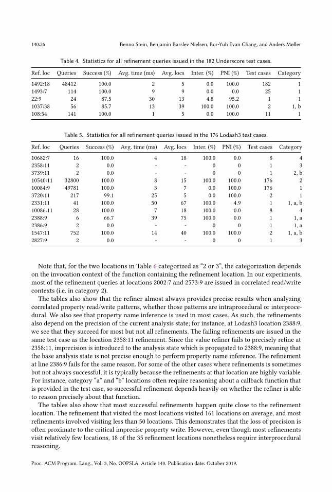
140:26 Benno Stein, Benjamin Barslev Nielsen, Bor-Yuh Evan Chang, and Anders Mùller
Table 4. Statistics for all refinement queries issued in the 182 Underscore test cases.
Ref. loc Queries Success (%) Avg. time (ms) Avg. locs Inter. (%) PNI (%) Test cases Category
1492:18 48412 100.0 2 5 0.0 100.0 182 11493:7 114 100.0 9 9 0.0 0.0 25 122:9 24 87.5 30 13 4.8 95.2 1 11037:38 56 85.7 13 39 100.0 100.0 2 1, b108:54 141 100.0 1 5 0.0 100.0 11 1
Table 5. Statistics for all refinement queries issued in the 176 Lodash3 test cases.
Ref. loc Queries Success (%) Avg. time (ms) Avg. locs Inter. (%) PNI (%) Test cases Category
10682:7 16 100.0 4 18 100.0 0.0 8 42358:11 2 0.0 - - 0 0 1 33739:11 2 0.0 - - 0 0 1 2, b10540:11 32800 100.0 8 15 100.0 100.0 176 210084:9 49781 100.0 3 7 0.0 100.0 176 13720:11 217 99.1 25 5 0.0 100.0 2 12331:11 41 100.0 50 67 100.0 4.9 1 1, a, b10086:11 28 100.0 7 18 100.0 0.0 8 42388:9 6 66.7 39 75 100.0 0.0 1 1, a2386:9 2 0.0 - - 0 0 1 1, a1547:11 752 100.0 14 40 100.0 100.0 2 1, a, b2827:9 2 0.0 - - 0 0 1 3
Note that, for the two locations in Table 6 categorized as ł2 or 3ž, the categorization dependson the invocation context of the function containing the refinement location. In our experiments,most of the refinement queries at locations 2002:7 and 2573:9 are issued in correlated read/writecontexts (i.e. in category 2).The tables also show that the refiner almost always provides precise results when analyzing
correlated property read/write patterns, whether those patterns are intraprocedural or interproce-dural. We also see that property name inference is used in most cases. As such, the refinementsalso depend on the precision of the current analysis state; for instance, at Lodash3 location 2388:9,we see that they succeed for most but not all refinements. The failing refinements are issued in thesame test case as the location 2358:11 refinement. Since the value refiner fails to precisely refine at2358:11, imprecision is introduced to the analysis state which is propagated to 2388:9, meaning thatthe base analysis state is not precise enough to perform property name inference. The refinementat line 2386:9 fails for the same reason. For some of the other cases where refinements is sometimesbut not always successful, it is typically because the refinements at that location are highly variable.For instance, category łaž and łbž locations often require reasoning about a callback function thatis provided in the test case, so successful refinement depends heavily on whether the refiner is ableto reason precisely about that function.The tables also show that most successful refinements happen quite close to the refinement
location. The refinement that visited the most locations visited 161 locations on average, and mostrefinements involved visiting less than 50 locations. This demonstrates that the loss of precision isoften proximate to the critical imprecise property write. However, even though most refinementsvisit relatively few locations, 18 of the 35 refinement locations nonetheless require interproceduralreasoning.
Proc. ACM Program. Lang., Vol. 3, No. OOPSLA, Article 140. Publication date: October 2019.

Static Analysis with Demand-Driven Value Refinement 140:27
Table 6. Statistics for all refinement queries issued in the 306 Lodash4 test cases.
Ref. loc Queries Success (%) Avg. time (ms) Avg. locs Inter. (%) PNI (%) Test cases Category
15702:9 291417 100.0 5 7 0.0 100.0 306 116840:11 99498 100.0 8 17 100.0 100.0 306 22573:9 500 89.6 361 97 100.0 97.1 14 2 or 315704:11 84 100.0 51 14 0.0 0.0 10 416983:7 45 97.8 32 40 100.0 0.0 12 42002:7 1209 94.7 1229 161 100.0 0.0 16 2 or 312808:13 164 100.0 4 5 0.0 100.0 1 1
Table 7. Statistics for all refinement queries issued in the 6 Prototype test cases.
Ref. loc Queries Success (%) Avg. time (ms) Avg. locs Inter. (%) PNI (%) Test cases Category
145:7 1102 100.0 13 40 46.8 100.0 6 17155:5 13 100.0 3 5 100.0 0.0 6 47157:5 4 100.0 4 5 100.0 0.0 3 43380:9 10 100.0 3 5 100.0 0.0 3 1, a
Table 8. Statistics for all refinement queries issued in the Scriptaculous test case.
Ref. loc Queries Success (%) Avg. time (ms) Avg. locs Inter. (%) PNI (%) Test cases Category
145:7 597 100.0 13 37 41.9 100.0 1 17155:5 4 100.0 4 5 100.0 0.0 1 4
Table 9. Statistics for all refinement queries issued in the JQuery test cases.
Ref. loc Queries Success (%) Avg. time (ms) Avg. locs Inter. (%) PNI (%) Test cases Category
368:6 8 87.5 85 26 0.0 0.0 8 18369:4 5 0.0 - - 0 0 5 1, a5188:4 2 0.0 - - 100.0 0.0 1 35200:4 63 100.0 5 5 0.0 100.0 1 13650:3 2 0.0 - - 0 0 1 3
ACKNOWLEDGMENTS
We are grateful to Esben Andreasen for his contributions to the early phases of this research. Thiswork was supported by the European Research Council (ERC) under the European Union’s Horizon2020 research and innovation program (grant agreement No 647544) and in part by NSF undergrants CCF-1619282 and CCF-1055066 and by DARPA under agreement number FA8750-14-2-0263.
REFERENCES
Roberto Amadini, Alexander Jordan, Graeme Gange, François Gauthier, Peter Schachte, Harald Sùndergaard, Peter J. Stuckey,and Chenyi Zhang. 2017. Combining String Abstract Domains for JavaScript Analysis: An Evaluation. In Tools and
Algorithms for the Construction and Analysis of Systems - 23rd International Conference, TACAS 2017 (Lecture Notes in
Computer Science), Vol. 10205. 41ś57.Esben Andreasen and Anders Mùller. 2014. Determinacy in Static Analysis for jQuery. In Proceedings of the 2014 ACM
International Conference on Object Oriented Programming Systems Languages & Applications, OOPSLA 2014. ACM, 17ś31.Esben Sparre Andreasen, Anders Mùller, and Benjamin Barslev Nielsen. 2017. Systematic Approaches for Increasing
Soundness and Precision of Static Analyzers. In Proceedings of the 6th ACM SIGPLAN International Workshop on State Of
the Art in Program Analysis, SOAP@PLDI 2017. 31ś36.
Proc. ACM Program. Lang., Vol. 3, No. OOPSLA, Article 140. Publication date: October 2019.

140:28 Benno Stein, Benjamin Barslev Nielsen, Bor-Yuh Evan Chang, and Anders Mùller
Thomas Ball, Orna Kupferman, and Greta Yorsh. 2005. Abstraction for Falsification. In Computer Aided Verification, 17th
International Conference, CAV 2005 (Lecture Notes in Computer Science), Vol. 3576. Springer, 67ś81.Thomas Ball and Sriram K. Rajamani. 2001. Automatically Validating Temporal Safety Properties of Interfaces. In Model
Checking Software, 8th International SPINWorkshop, 2001 (Lecture Notes in Computer Science), Vol. 2057. Springer, 103ś122.Sam Blackshear, Bor-Yuh Evan Chang, and Manu Sridharan. 2013. Thresher: Precise Refutations for Heap Reachability. In
Proc. ACM SIGPLAN Conference on Programming Language Design and Implementation. 275ś286.Satish Chandra, Stephen J. Fink, and Manu Sridharan. 2009. Snugglebug: A Powerful Approach to Weakest Preconditions.
In Proceedings of the 2009 ACM SIGPLAN Conference on Programming Language Design and Implementation, PLDI 2009.ACM, 363ś374.
Bor-Yuh Evan Chang and K. Rustan M. Leino. 2005. Abstract Interpretation with Alien Expressions and Heap Structures. InVerification, Model Checking, and Abstract Interpretation, 6th International Conference, VMCAI 2005. 147ś163.
David R. Chase, Mark N. Wegman, and F. Kenneth Zadeck. 1990. Analysis of Pointers and Structures. In Proceedings of the
ACM SIGPLAN’90 Conference on Programming Language Design and Implementation, PLDI 1990. ACM, 296ś310.Edmund M. Clarke, Orna Grumberg, Somesh Jha, Yuan Lu, and Helmut Veith. 2000. Counterexample-Guided Abstraction
Refinement. In Computer Aided Verification, 12th International Conference, CAV 2000 (Lecture Notes in Computer Science),Vol. 1855. Springer, 154ś169.
Patrick Cousot and Radhia Cousot. 1977. Abstract Interpretation: A Unified Lattice Model for Static Analysis of Programsby Construction or Approximation of Fixpoints. In Conference Record of the Fourth ACM Symposium on Principles of
Programming Languages, POPL 1977. ACM, 238ś252.Patrick Cousot and Radhia Cousot. 1979. Systematic Design of Program Analysis Frameworks. In Conference Record of the
Sixth Annual ACM Symposium on Principles of Programming Languages POPL 1979. 269ś282.Patrick Cousot and Radhia Cousot. 1992. Abstract Interpretation Frameworks. J. Log. Comput. 2, 4 (1992), 511ś547.Patrick Cousot, Radhia Cousot, Jérôme Feret, Laurent Mauborgne, Antoine Miné, David Monniaux, and Xavier Rival. 2006.
Combination of Abstractions in the ASTRÉE Static Analyzer. In Advances in Computer Science - ASIAN 2006. Secure
Software and Related Issues, 11th Asian Computing Science Conference (Lecture Notes in Computer Science), Vol. 4435.Springer, 272ś300.
Patrick Cousot, Radhia Cousot, and Francesco Logozzo. 2011. Precondition Inference from Intermittent Assertions andApplication to Contracts on Collections. In Verification, Model Checking, and Abstract Interpretation - 12th International
Conference, VMCAI 2011. 150ś168.Arlen Cox, Bor-Yuh Evan Chang, and Xavier Rival. 2014. Automatic Analysis of Open Objects in Dynamic Language
Programs. In Static Analysis - 21st International Symposium, SAS 2014. 134ś150.Kyle Dewey, Vineeth Kashyap, and Ben Hardekopf. 2015. A Parallel Abstract Interpreter for JavaScript. In Proceedings of
the 13th Annual IEEE/ACM International Symposium on Code Generation and Optimization, CGO 2015. IEEE ComputerSociety, 34ś45.
Cormac Flanagan, K. Rustan M. Leino, Mark Lillibridge, Greg Nelson, James B. Saxe, and Raymie Stata. 2002. ExtendedStatic Checking for Java. In Proceedings of the 2002 ACM SIGPLAN Conference on Programming Language Design and
Implementation (PLDI). ACM, 234ś245.Philippa Gardner, Sergio Maffeis, and Gareth David Smith. 2012. Towards a Program Logic for JavaScript. In Proceedings of
the 39th ACM SIGPLAN-SIGACT Symposium on Principles of Programming Languages, POPL 2012. 31ś44.Arjun Guha, Claudiu Saftoiu, and Shriram Krishnamurthi. 2010. The Essence of JavaScript. In ECOOP 2010 - Object-Oriented
Programming, 24th European Conference, Proceedings. Springer, 126ś150.Bhargav S. Gulavani and Sriram K. Rajamani. 2006. Counterexample Driven Refinement for Abstract Interpretation. In Tools
and Algorithms for the Construction and Analysis of Systems, 12th International Conference, TACAS 2006 (Lecture Notes in
Computer Science), Vol. 3920. Springer, 474ś488.Samuel Z. Guyer and Calvin Lin. 2005. Error Checking with Client-Driven Pointer Analysis. Sci. Comput. Program. 58, 1-2
(2005), 83ś114.Thomas A. Henzinger, Ranjit Jhala, Rupak Majumdar, and Grégoire Sutre. 2002. Lazy Abstraction. In Conference Record of
POPL 2002: The 29th SIGPLAN-SIGACT Symposium on Principles of Programming Languages. ACM, 58ś70.IBM Research. 2018. T.J. Watson Libraries for Analysis (WALA).Samin S. Ishtiaq and Peter W. O’Hearn. 2001. BI as an Assertion Language for Mutable Data Structures. In Conference Record
of POPL 2001: The 28th ACM SIGPLAN-SIGACT Symposium on Principles of Programming Languages. ACM, 14ś26.Simon Holm Jensen, Anders Mùller, and Peter Thiemann. 2009. Type Analysis for JavaScript. In Static Analysis, 16th
International Symposium, SAS 2009 (Lecture Notes in Computer Science), Vol. 5673. Springer, 238ś255.John B. Kam and Jeffrey D. Ullman. 1977. Monotone Data Flow Analysis Frameworks. Acta Inf. 7 (1977), 305ś317.Vineeth Kashyap, Kyle Dewey, Ethan A. Kuefner, John Wagner, Kevin Gibbons, John Sarracino, Ben Wiedermann, and Ben
Hardekopf. 2014. JSAI: A Static Analysis Platform for JavaScript. In Proc. 22nd ACM SIGSOFT International Symposium on
Foundations of Software Engineering. 121ś132.
Proc. ACM Program. Lang., Vol. 3, No. OOPSLA, Article 140. Publication date: October 2019.

Static Analysis with Demand-Driven Value Refinement 140:29
Gary A. Kildall. 1973. A Unified Approach to Global Program Optimization. In Conference Record of the ACM Symposium on
Principles of Programming Languages, POPL 1973. ACM Press, 194ś206.Yoonseok Ko, Xavier Rival, and Sukyoung Ryu. 2017. Weakly Sensitive Analysis for Unbounded Iteration over JavaScript
Objects. In Programming Languages and Systems - 15th Asian Symposium, APLAS 2017. 148ś168.Yoonseok Ko, Xavier Rival, and Sukyoung Ryu. 2019. Weakly Sensitive Analysis for JavaScript Object-Manipulating
Programs. Softw., Pract. Exper. 49, 5 (2019), 840ś884.Hongki Lee, Sooncheol Won, Joonho Jin, Junhee Cho, and Sukyoung Ryu. 2012. SAFE: Formal Specification and Imple-
mentation of a Scalable Analysis Framework for ECMAScript. In Proc. International Workshop on Foundations of Object
Oriented Languages (FOOL 2012).Sorin Lerner, David Grove, and Craig Chambers. 2002. Composing Dataflow Analyses and Transformations. In Conference
Record of POPL 2002: The 29th SIGPLAN-SIGACT Symposium on Principles of Programming Languages. 270ś282.Percy Liang and Mayur Naik. 2011. Scaling Abstraction Refinement via Pruning. In Proceedings of the 32nd ACM SIGPLAN
Conference on Programming Language Design and Implementation, PLDI 2011. 590ś601.Magnus Madsen and Esben Andreasen. 2014. String Analysis for Dynamic Field Access. In Proc. 23rd International Conference
on Compiler Construction (Lecture Notes in Computer Science), Vol. 8409. Springer.Roman Manevich, Manu Sridharan, Stephen Adams, Manuvir Das, and Zhe Yang. 2004. PSE: Explaining Program Failures
via Postmortem Static Analysis. In Proceedings of the 12th ACM SIGSOFT International Symposium on Foundations of
Software Engineering, FSE 2004. ACM, 63ś72.Hakjoo Oh, Wonchan Lee, Kihong Heo, Hongseok Yang, and Kwangkeun Yi. 2016. Selective X-Sensitive Analysis Guided by
Impact Pre-Analysis. ACM Trans. Program. Lang. Syst. 38, 2 (2016), 6:1ś6:45.Changhee Park, Hyeonseung Im, and Sukyoung Ryu. 2016. Precise and Scalable Static Analysis of jQuery using a Regular
Expression Domain. In Proceedings of the 12th Symposium on Dynamic Languages, DLS 2016. ACM, 25ś36.Changhee Park and Sukyoung Ryu. 2015. Scalable and Precise Static Analysis of JavaScript Applications via Loop-Sensitivity.
In Proc. 29th European Conference on Object-Oriented Programming. 735ś756.Xavier Rival and Laurent Mauborgne. 2007. The Trace Partitioning Abstract Domain. ACM Trans. Program. Lang. Syst. 29, 5
(2007), 26.José Fragoso Santos, Petar Maksimovic, Daiva Naudziuniene, Thomas Wood, and Philippa Gardner. 2018. JaVerT: JavaScript
Verification Toolchain. PACMPL 2, POPL (2018), 50:1ś50:33.José Fragoso Santos, Petar Maksimovic, Gabriela Sampaio, and Philippa Gardner. 2019. JaVerT 2.0: Compositional Symbolic
Execution for JavaScript. PACMPL 3, POPL (2019), 66:1ś66:31.Johannes Späth, Lisa Nguyen Quang Do, Karim Ali, and Eric Bodden. 2016. Boomerang: Demand-Driven Flow- and
Context-Sensitive Pointer Analysis for Java. In 30th European Conference on Object-Oriented Programming, ECOOP 2016.22:1ś22:26.
Manu Sridharan and Rastislav Bodík. 2006. Refinement-Based Context-Sensitive Points-To Analysis for Java. In Proceedings
of the ACM SIGPLAN 2006 Conference on Programming Language Design and Implementation, PLDI 2006. 387ś400.Manu Sridharan, Julian Dolby, Satish Chandra, Max Schäfer, and Frank Tip. 2012. Correlation Tracking for Points-To
Analysis of JavaScript. In Proc. 26th European Conference on Object-Oriented Programming.Antoine Toubhans, Bor-Yuh Evan Chang, and Xavier Rival. 2013. Reduced Product Combination of Abstract Domains for
Shapes. In Verification, Model Checking, and Abstract Interpretation, 14th International Conference, VMCAI 2013. 375ś395.Shiyi Wei, Omer Tripp, Barbara G. Ryder, and Julian Dolby. 2016. Revamping JavaScript Static Analysis via Localization
and Remediation of Root Causes of Imprecision. In Proceedings of the 24th ACM SIGSOFT International Symposium on
Foundations of Software Engineering, FSE 2016. ACM, 487ś498.
Proc. ACM Program. Lang., Vol. 3, No. OOPSLA, Article 140. Publication date: October 2019.