State Tax Revenue Growth and Volatility · State Tax Revenue Growth and Volatility Gary C. Cornia...

State Tax Revenue Growth and Volatility

Gary C. Cornia and Ray D. Nelson

broader bases generate significant increases in taxrevenues and often lead to new or broader financialcommitments. However, when the economy lapsesinto recessionary conditions, these commitmentsinevitably contribute to higher levels of budgetarystress. The resulting budget deficits once againchallenge state officials to find new revenue sourcesand cut expenditures.

Sobel and Wagner (2003) suggest that, whenchanging the tax code to generate additional rev-enue, government officials and public policymakersshould consider the implications of such revisionson the long-run expected growth and volatility oftax revenues. Highly volatile taxes or taxes withhigh income elasticities are useful when trying tobalance a budget but create substantial challengeswhen the economy contracts. What increases rap-idly during an economic expansion also falls pre-cipitously during an economic contraction. Theresulting challenge of revenue shortfalls during adownturn is especially acute in the current eco-

In recent years, state legislators and governorsfaced difficult budget deliberations causedby revenue shortfalls. News reports repeat-edly identify and chronicle the dire fiscal

conditions faced by most states. Dadayan andBoyd (2009) report record drops in tax revenuesand describe historically difficult budgeting con-ditions. Unfortunately, if the patterns continue,states will yet face severe budgeting challengesbeyond the official end of the national recession.These challenges will be especially acute if a slug-gish labor market recovery and renewed bankingsector stress persistently retard sales and incometax receipts.

Gamage (forthcoming) identifies a recurrentpattern of state fiscal crises. He describes how statesoften broaden tax bases or raise tax rates duringrecessions to maintain commitments made duringprosperous periods. When the economy begins torecover, states experience budgetary relief as taxrevenues grow. Eventually, the higher rates and

Macroeconomic conditions and tax structures jointly determine the growth and volatility of statetax revenues. Since a variety of economic conditions exist among states, government policymakersshould carefully anticipate and consider the possible impacts of proposed tax reform and revenueenhancements on the long-term growth and volatility of their unique tax revenue portfolios. In theshort run, states generally cannot alter the volatility and growth rates of their economies. They can,however, change the composition of their tax portfolios to minimize the effects of the businesscycle on their fiscal health. For this reason, state officials need to consider the natural tendenciesof their economies when formulating tax policy. For example, states with volatile economies mightwant tax portfolios that minimize the impact of national macroeconomic trends; those with stableeconomies might consider adopting more aggressive tax portfolios that optimize their tax revenuegrowth/volatility combinations. (JEL H21, H72, R51)

Federal Reserve Bank of St. Louis Regional Economic Development, 2010, 6(1), pp. 23-58.

FEDERAL RESERVE BANK OF ST. LOUIS REGIONAL ECONOMIC DEVELOPMENT VOLUME 6, NUMBER 1 2010 23

Gary C. Cornia is dean and Ray D. Nelson is an associate professor at the Marriott School of Management, Brigham Young University.

© 2010, The Federal Reserve Bank of St. Louis. The views expressed in this article are those of the author(s) and do not necessarily reflect theviews of the Federal Reserve System, the Board of Governors, or the regional Federal Reserve Banks. Articles may be reprinted, reproduced,published, distributed, displayed, and transmitted in their entirety if copyright notice, author name(s), and full citation are included. Abstracts,synopses, and other derivative works may be made only with prior written permission of the Federal Reserve Bank of St. Louis.

24 VOLUME 6, NUMBER 1 2010 FEDERAL RESERVE BANK OF ST. LOUIS REGIONAL ECONOMIC DEVELOPMENT

nomic and political environment. Although eco-nomic discussions of taxes almost always includeconsideration of the important principles of equity,efficiency, and economic development, the goal ofbalancing budgets currently trumps almost everyother policy dimension.

Two main factors affect the growth and volatil-ity of state tax revenue receipts over the businesscycle. First, the uniqueness of each state’s economyultimately affects its growth and volatility. Second,a state’s choice of taxes, tax base, and tax rates canalter the revenue growth and volatility inherent inits economy. Because macroeconomic conditionsvary so widely among states, subnational govern-ment officials must wisely consider the growth andvolatility of their unique tax portfolio to minimizefuture fiscal challenges.

Legislative and executive tax policy can benefitfrom answers to the following research questions:

(i) How can state economic growth andvolatility be accurately measured andconsistently compared?

(ii) How do alternative revenue sources con-tribute to the growth and volatility of rev-enues generated by state tax portfolios?

(iii) How do state economies and tax portfoliosinteract to determine tax revenue growthand volatility?

The paper proceeds as follows. Analysis of thethree questions first considers patterns in the U.S.business cycle and subsequently focuses on thevariety of economic conditions experienced byindividual states. Examination of the growth andvolatility of individual tax sources, especially sales,income, and property taxes, suggests their poten-tially differing effects on revenue growth and sta-bility. Inquiries into tax volatility are guided bybuilding on the literature initiated by Groves andKahn (1952). Two illustrations then demonstratehow knowledge of tax revenue growth and volatilitycan be incorporated into budgeting decisions andpublic policy. Because the growth and volatility oftax receipts likely depend on economic conditionsand tax policy, the analysis of historical patternshelps identify best practices among states. Suchanalysis can potentially help decisionmakers knowwhich growth and volatility characteristics have

helped states weather the current fiscal storm.Finally, the analysis here makes practical recom-mendations based on a summary of empirical find-ings and research conclusions.

This article uses simple graphical constructsto summarize extensive data resources. Hopefully,this approach will foster insights that governmentofficials and budget analysts might find useful intheir tax reform and budget balancing efforts. Ofcourse, more sophisticated statistical models arepossible and appropriate for future work. The sim-plicity of the graphical tools and data explorationphilosophy pioneered by Tukey (1977) and refinedby Tufte (2001), however, increases the probabilitythat policymakers and their respective professionalstaffs will use the findings of the present researcheffort. In the past, similar graphical communicationhas proven very successful and influential in help-ing executive and legislative branch officials under-stand empirical findings critical for tax policy.

HISTORICAL BACKGROUNDHolcombe and Sobel (1997) and Crain (2003)

emphasize the importance of including theexpected growth rates and volatility of revenuesand expenditures whenever conducting fiscalanalysis. Their comments suggest that the first stepin understanding revenue growth and volatility isto consider the macroeconomic background thatgenerates the revenue streams.

Recent Macroeconomic Patterns

Researchers commonly focus on the NationalBureau of Economic Research (NBER) BusinessCycle Dating Committee’s declarations when study-ing business cycles. NBER leading, coincident, andlagging indicators establish the beginning, end, andduration of national expansions and recessions.The NBER cycle analysis works well at the nationallevel. However, because state business cycles donot synchronize perfectly with national patterns,state-level measures are needed to make interstatebusiness cycle comparisons. Fortunately, theFederal Reserve Bank of Philadelphia publishesmonthly coincident indexes that measure eachstate’s economic activity in a consistent fashion.

Cornia and Nelson

The Philadelphia indexes provide insightfulindicators for anticipating state tax revenues. Themethodology implemented by the PhiladelphiaFed builds on the pioneering work of Stock andWatson (1989). Crone and Clayton-Matthews (2005)adapt this methodology to state-level data. Theycollapse (i) nonfarm payroll employment, (ii)average hours worked in manufacturing, (iii) theunemployment rate, and (iv) real wage and salarydisbursements into a single index by using adynamic single-factor model. The method uses aKalman filter to extract a major component fromeach of these four different time series. With thisapproach the trend for each state’s index is set tothe trend of its gross state product. With carefulimplementation, the long-term growth in a state’s

index closely tracks the state’s overall business-cycle patterns. Because the model and the inputvariables are consistent across all 50 states, theresulting state indexes are comparable.

The Philadelphia Fed also constructs a nationalcoincident index that provides growth and volatil-ity data for the U.S. economy—a useful startingpoint for evaluating the potential influences ontotal state receipts. Figure 1 shows the year-over-year growth rate in the national coincident index.The five recessions shown vary significantly intheir severity and duration. According to NBERbusiness cycle dating protocol, a very brief and mildrecession began in July 1990 and ended in March1991. Once a vigorous expansion began, the econ-omy accelerated into the longest post-World War IIexpansion on record.

Cornia and Nelson


1980 1985 1990 1995 2000 2005 2010–10

–5

0

5

10

Smoothed Trends (locally weighted scatterplot smoothing [LOWESS])

Year-Over-Year Percentage Change

Percentage Change

Figure 1

The U.S. Business Cycle and Year-Over-Year Growth Rate of the National Coincident Index (1979-2009)

SOURCE: Federal Reserve Bank of Philadelphia State Coincident Indexes.


Cornia and Nelson

of jobs lost since the beginning of the recession.The depth of the decline makes some economistspessimistic about the time it will take for labormarkets to return to employment levels achievedduring the previous expansion.

State Tax Revenues and the BusinessCycle

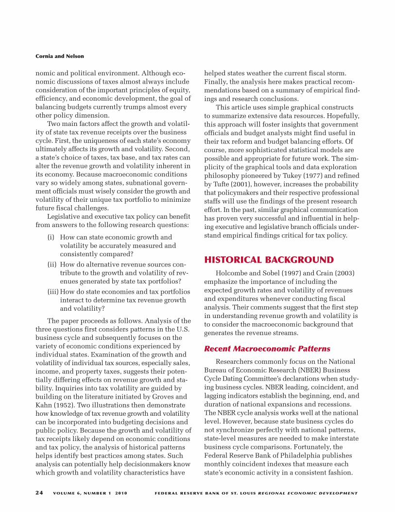
Total state tax revenues as estimated by theCensus Bureau show the current fiscal dilemmafaced by many states. Figure 2 demonstrates howtotal state tax revenues vary over the business cycle.The blue line corresponds to the rate of changein the year-over-year national coincident indexshown in Figure 1. Adjusting each tax revenue timeseries by the Personal Consumption ExpenditureIndex gives real rates that are comparable to the

Similarly, another brief and mild recessionbegan during March 2001 and officially ended inNovember 2001. In contrast to the previous busi-ness cycle, the economy did not recover rapidlyafter that recession. The figure, which reflects thelarge emphasis on labor market conditions in thePhiladelphia Fed index, show that a jobless recov-ery continued almost two years after the recessionofficially ended.

The present recession that according to theNBER began in December 2007 is noteworthybecause of its depth and length. The national coin-cident index did not fall below the previous year’slevel until a few months after that start date. Thedepth of the fall is the worst since the GreatDepression. Because of the prominent weightingof labor markets in the index, it reflects the millions

1990 1995 2000 2005 2010

–20

–10

0

10

Smoothed Revenues (LOWESS)

Year-Over-Year Revenue Percentage Change

Smoothed National Index (LOWESS)

Percentage Change

Figure 2

Total State Tax Revenues Over the Business Cycle: Year-Over-Year Growth Rates (1989-2009)

SOURCE: Federal Reserve Bank of Philadelphia State Coincident Indexes and Census Bureau Quarterly State and Local Government TaxRevenue.


Cornia and Nelson

gled to improve. This jobless recovery undoubtedlytranslated into the slow growth in state tax rev-enues. Eventually, tax receipts accelerated rapidlyand even exceeded growth in the U.S. economysubstantially until partway through the next reces-sion. During one quarter, the year-over-year growthrate for total state tax revenues exceeded 15 percent.During the most recent recession, state tax rev-enues decreased dramatically relative to the U.S.economy, which corresponds to the unprecedented,record-breaking decline mentioned by Dadayanand Boyd (2009).

The box plots in Figure 3 facilitate comparisonof the distributions of the changes in state tax rev-enues and the U.S economy. These plots succinctlysummarize the location and spread of each distri-

real national coincident index growth rates.Interestingly, state tax revenues, shown in red,declined more rapidly than the U.S. economy (asdepicted by the national coincident index) in eachbusiness cycle. In the recession that began in 1991,neither the magnitude nor duration of declines inrevenues were significant enough to cause severebudgeting challenges. As would be expected, rev-enues increased over the entire record-long expan-sion of the Clinton administration, at times at arate well in excess of that for the U.S. economy.However, during three different periods, revenuesdeclined at a rate greater than that for the U.S.economy.

In the recovery from the 2001 recession, the U.S.economy grew slowly and the labor market strug-

Percentage

U.S. Economy

State Tax Revenues

–15 5 5 15

Figure 3

State Tax Revenues versus the U.S. Economy: Year-Over-Year Growth Rates in QuarterlyObservations (1989-2009)


Cornia and Nelson


–40 –30 –2 –10 0 10

Percentage

1 MI2 HI3 AK4 LA5 MO6 ME7 OH8 AL9 WI

10 KS11 MS12 IN13 WY14 IL15 NE16 ND17 AR18 KY19 NJ20 PA21 MD22 SD23 TN24 VT25 DE26 US27 IA28 NM29 WV30 OK31 MN32 NY33 CT34 VA35 NC36 RI37 MT38 SC39 CO40 GA41 MA42 NH43 WA44 CA45 FL46 TX47 OR48 UT49 ID50 AZ51 NV

Figure 4A

State Economies: Year-Over-Year Growth Rates in Monthly Coincident Indexes Ranked by Medianof Percentage Change (1995-2009)


Cornia and Nelson


1 NM2 ND3 US4 AK5 TN6 RI7 MT8 WI9 VA

10 SD11 AR12 KY13 NE14 FL15 OK16 NC17 IN18 WV19 MS20 NJ21 TX22 OH23 LA24 ME25 CA26 MD27 IA28 KS29 MA30 ID31 CO32 WY33 GA34 MO35 SC36 NH37 IL38 VT39 CT40 HI41 MN42 PA43 UT44 DE45 AL46 AZ47 NY48 WA49 NV50 MI51 OR

–40 –30 –2 –10 0 10

Percentage

Figure 4B

State Economies: Year-Over-Year Growth Rates in Monthly Coincident Indexes Ranked byInterquartile Range of Percentage Change (1995-2009)


bution by using first, second, and third quartiles.The median of the distributions is depicted by thedot in the middle of the notched box. The lengthof the box depicts the interquartile range (IQR),the difference between the third and first quartiles,and is one measure of the distributions’ spread.Put another way, the middle 50 percent of obser-vations lie in the range encompassed by the box.The whiskers give another measure of the spreadand bracket all observations within 1.5 * IQR dis-tance from the sides, or hinges, of the box. In therevenue box plot, the large and small observationsoutside the whisker boundaries are classified asoutliers and correspond to quarters when revenueeither fell precipitously or grew rapidly.

Figures 2 and 3 support the conclusion thatthe average rates of change in state tax revenuesand the U.S. economy are equal but more volatilefor revenues. First, in Figure 3, the middle (median)of the box plot for revenues is slightly less thanthat for the economy. Second, half of the increasesin revenue exceed the largest increase in the econ-omy. This means that the size of state governmentsincreased relative to the U.S. economy during theperiod 1994-2009. The box plots also suggest thatgrowth of revenues is more volatile and negativelyskewed than growth of the economy. Both the widthof the IQR and the length of the whiskers show thatrevenues have a bigger spread than the economy.Although revenues and the economy both haveextreme increases and decreases as indicated bythe outliers, the negative skewness conclusion forrevenues follows because the number of extremedeclines in revenues exceeds that for the economy.The fact that measures of state tax revenue growthand volatility both exceed similar measures for theU.S. economy suggests that state budgets are veryexposed and susceptible to potential economicdownturns.

Individual State Growth and VolatilityDuring the National Business Cycle

To make budgeting and policy recommenda-tions for individual states, it is important to questionwhether national patterns generalize to individualstates. Another interesting investigation exploresthe possible trade-off between growth and volatil-ity (Groves and Kahn, 1952). Previous work by

Crain (2003) investigates whether the expectedreturn and risk trade-off found in financial marketssimilarly applies to the relationship between astate’s economic growth and volatility and its taxrevenues.

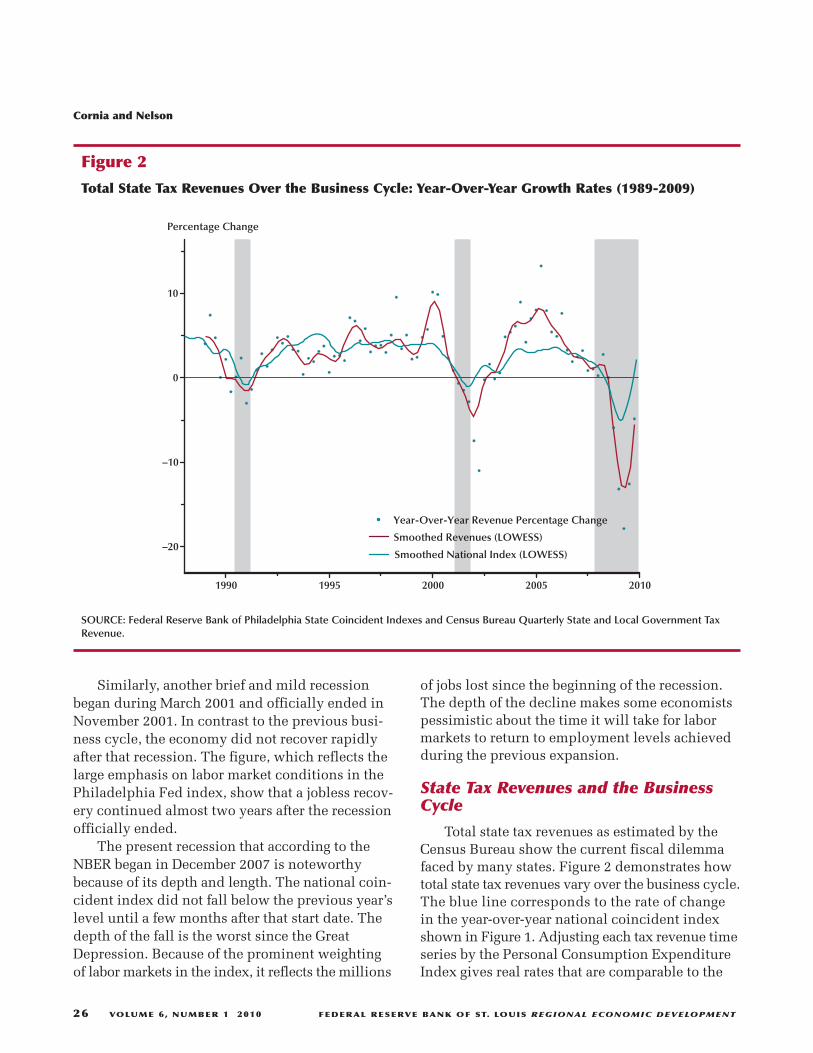
The box plots in Figures 4A and 4B lead to rel-evant observations about the growth and volatilityof individual state economies. The plots depict thedistribution of year-over-year percentage changesin the Philadelphia coincident index for eachindividual state and for the U.S. economy. Thetwo plots differ only in their criterion for ranking.Figure 4A is ranked by the median growth rate ofthe coincident index for each state.

As would be expected, in Figure 4A the UnitedStates ranks in the middle (26th) simply becauseit is the weighted average of all states. Because ofthe number of extreme negative observations dur-ing the current recession, all of the means tend topull toward the left side of the box and whisker dia-gram. This is consistent with a negatively skeweddistribution for the rates of change. The number ofnegative outliers shows that all states suffered atleast some extreme declines in their economiesduring the period 1995-2009.

The box plots in Figure 4B focus on volatilityrather than growth. Figure 4B presents the sameinformation as in Figure 4A, except each state isnow ranked by the IQR rather than the median.Figure 4B identifies Oregon, Michigan, Nevada,Washington, and New York as having volatileeconomies. As expected, the United States, a port-folio of all states, has low volatility. New Mexico,North Dakota, Alaska, Tennessee, and Rhode Islandalso have relatively stable economies. Michigan isespecially noteworthy because it has a negativeaverage growth rate. Three large negative quartersfor Michigan pull the mean significantly down fromthe median. It is also interesting that its spreadshown by its IQR and the length of the whiskersimply that the Michigan economy is also veryvolatile. Michigan does not have the benefit of ahigh growth rate to compensate for its high volatil-ity. This contrasts with the high-growth and high-volatility combinations evident for Oregon,Washington, and Nevada.

Despite the attention California receives in thepopular press, its economy does not exhibit extreme

Cornia and Nelson


volatility, even though it does have a very highgrowth rate. As expected because of their geographi-cal proximity, Washington and Oregon seem toexhibit similar characteristics. Two states that heav-ily depend on energy extraction, Wyoming andAlaska, have low growth rates. Alaska, however,does not endure the same extreme variability ineconomic growth that Wyoming does. Texas dis-tinguishes itself with its desirable combination ofhigh growth and low volatility.

The Efficiency Frontier for StateEconomies

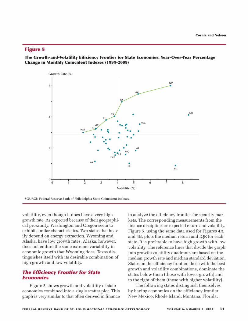
Figure 5 shows growth and volatility of stateeconomies combined into a single scatter plot. Thisgraph is very similar to that often derived in finance

to analyze the efficiency frontier for security mar-kets. The corresponding measurements from thefinance discipline are expected return and volatility.Figure 5, using the same data used for Figures 4Aand 4B, plots the median return and IQR for eachstate. It is preferable to have high growth with lowvolatility. The reference lines that divide the graphinto growth/volatility quadrants are based on themedian growth rate and median standard deviation.States on the efficiency frontier, those with the bestgrowth and volatility combinations, dominate thestates below them (those with lower growth) andto the right of them (those with higher volatility).

The following states distinguish themselvesby having economies on the efficiency frontier:New Mexico, Rhode Island, Montana, Florida,

Cornia and Nelson


00 1 2 3 4 5 6 7 8

2

4

6

HI

NV

AZ

ID

TX

FL

MTRI

NM

AK

MI

OR

WA

AL

LAMO

OH

Growth Rate (%)

Volatility (%)

Figure 5

The Growth-and-Volatility Efficiency Frontier for State Economies: Year-Over-Year PercentageChange in Monthly Coincident Indexes (1995-2009)


Texas, Idaho, Arizona, and Nevada. States thatseem to have inferior combinations of low growthand high volatility are Michigan, Alabama, Hawaii,and Missouri. Alaska, Ohio, and Louisiana fit intothe low-growth/low-volatility quadrant. Somestates that have widely reported and especiallyacute fiscal challenges—California for example —surprisingly have relatively stable economies andmoderate growth rates.

DIVERSITY AMONG STATE TAXPORTFOLIOS

The second determinant of state tax revenuegrowth and volatility comes from the characteris-tics of individual taxes. Each state selects its ownset of revenue sources, which it combines into itstax portfolio. In addition, each state chooses itstax base and corresponding tax rates.

The Constitution of the United States allowssubstantial freedom for states to adopt differenttax schemes. The variety of adopted tax policiesreflects a wide spectrum of political preferencesamong state populations. The state of Oregon, forexample, has resisted adopting a retail sales tax.This contrasts with a neighboring state, Washington,which has a retail sales tax but no income tax. Evenamong the 44 states that have a retail sales tax, itsimplementation is far from uniform. Retail sales taxrates range from below 4 percent to double digits.Sales tax bases also show similar variety. About75 percent of states exempt food purchases fromthe retail sales tax. The desire to mediate the regres-sive nature of the retail sales tax motivates thisexemption. In many cases, however, the foodexemption eventually leads to higher rates on theremaining taxed goods. In most states, the retailsales tax base includes very few services; however,some states tax many services.

State individual income tax has a similar pat-tern of heterogeneity. A few states do not imposeany such income tax. Those states with an individ-ual income tax choose a variety of tax rates andbases. In general, most states start with the federalincome tax as the base but adopt different levelsof exemptions and deductions. Marginal tax ratesrange from under 5 percent to over 10 percent.

Some states have income brackets taxed at differentrates, whereas others apply one rate to all taxableincome. These differences in tax bases and ratescause state tax revenues to respond in a variety ofways to macroeconomic changes.

A standard theme in state tax design is to keeptax bases as broad as possible while keeping taxrates as low as possible. Many believe that broadbases and low rates generate less revenue growthduring economic upswings but also result in smallerrevenue shortfalls during economic downturns.

Although state tax portfolios vary significantly,most states rely on some combination of sales,individual income, and property taxes. Becauseproperty taxes primarily finance local governments,meaningful consideration of this potential revenuesource requires expanding the tax revenue defini-tion to include all state and local taxes. Otherwise,the resulting analysis would give a distorted viewof the property tax.

Growth and Volatility of IndividualState Taxes

As mentioned, business cycle phases causestate governments to regularly alter their tax struc-ture. Frequent and substantial changes to tax codesinfluence the growth rate and volatility of taxsources. Although calculating growth and volatil-ity estimates based on a uniform tax policy wouldyield accurate and informative results, such idealdata unfortunately do not exist. It is true that onemight try collecting fiscal note analyses for indi-vidual states to adjust for their tax rate and basechanges. Such an approach, however, suffers fromaccuracy and feasibility concerns. The inherentinaccuracy of fiscal note estimates can itself poten-tially bias growth and volatility estimates. Even iffiscal notes were totally accurate, however, thediversity of state analytical procedures would likelymake the task of collecting such data impractical.

For this reason, when interpreting and compar-ing growth and volatility estimates for various taxes,it is important to remember that (i) the growthrates and risk of each tax depend on the inherentcharacteristics of the tax category and (ii) the esti-mates also include the propensity of governmentofficials to alter the tax structure. As shown subse-quently, major and frequent changes to the tobacco

Cornia and Nelson


tax base and rate significantly influence the meanand standard deviation of tax revenues. For this rea-son, it is important to use resistant statistics (suchas medians and IQRs, as used here) to describe thehistorical distribution of rates of change. Thesestatistics can effectively exclude extreme rate andbase changes from the estimation process.

With the aforementioned caveats in mind, firstconsider possible differences in the growth andvolatility of individual taxes as measured by tra-ditional location and scale measures. The box plotin Figure 6A depicts the distribution of year-over-year changes in quarterly observations in the majortax categories reported by the Census Bureau. Thecategories in the box plot are ranked according tothe median percentage change in total revenue.Taxes on alcoholic beverages and motor fuels havelow growth rates. These two taxes are also verystable and provide states and local governmentswith a steady revenue source. Unfortunately, thesetaxes represent a very small portion of most states’general revenues.

Motor license taxes include vehicles anddrivers. As shown in Figures 6A and 6B, this cate-gory has the third-lowest growth rate among the10 revenue categories. Measuring the volatility asa standard deviation unfairly labels this tax revenuesource as relatively more volatile. The box andwhiskers, based on the resistant IQR statistics, indi-cate much less volatility. Three extremely large out-liers shown in Figures 6A and 6B unduly influencethe estimated standard deviation. A combinationof population growth and licensing fee increaseslikely explains the extreme increases in revenue.Less explainable is the one quarter of significantdecline.

The corporate income tax is especially problem-atic in state budgeting because of its high volatility.Interestingly, its high volatility is not associatedwith a high growth rate. From a similar point ofview used to analyze financial markets, this is ahigh-risk revenue source without compensationprovided by higher expected growth.

The “All Other” tax category exhibits high posi-tive skewness. This probably results from attemptsby legislative and executive branches to search for“low-hanging fruit” to augment tax revenues andhelp balance budgets during economic downturns.

As mentioned, the retail sales and gross receiptstax is a very significant revenue source for stateand local governments. As shown in Figures 6Aand 6B, it grows moderately relative to other taxrevenues and is also reasonably stable. It does havea couple of very negative growth quarters. Themean for this category is probably influenced bya series of three quarters of significantly largedeclines. In some states, the sales tax generatesover 50 percent of state revenues. In most states,however, the sales tax is less than 40 percent oftotal state revenues.

It is difficult to characterize how tobacco taxesrespond to the growth and volatility of the businesscycle because the tax rate on these products hasincreased so rapidly during the period covered bythese data. Tobacco taxes show extreme positivegrowth rates. This surely reflects significantincreases in tax rates applied to tobacco products.For this reason, the median and IQR rather thanthe mean and standard deviation much better sum-marize the growth and volatility of tobacco taxrevenues.

As mentioned, individual income taxes alsoconstitute a very important source of revenue forstate and local governments. Their growth rateexceeds that of the retail sales and gross receiptstaxes. It is also much more volatile. This volatilityis undoubtedly the source of many of the currentbudgeting challenges faced by state and local gov-ernments. Notice the large number of outliers,which correspond to negative rates of growth dur-ing the current recession. The significant numberof positive deviations possibly encouraged stateand local governments to increase their governmentexpenditures and base budgets.

The property tax is mainly used to financelocal government. Its combination of high growthand low volatility make it a very attractive revenuesource. Its high growth rate is undoubtedly relatedto the real estate bubble that existed during theearly part of this century. If real estate prices con-tinue to decline, however, the growth rate of theproperty tax could decline commensurately.

Consider now the diversification potential forstates of including multiple revenue sources withintheir tax portfolio. Combining the nine tax cate-gories in Figures 6A and 6B gives a portfolio with

Cornia and Nelson


the eighth-largest growth rate and third-smallestvolatility, respectively. This seems to indicate thatstates with a combination of taxes would tend todecrease the volatility of tax revenues withoutsacrificing expected growth. This result is consis-tent with the principles used to achieve diversifi-cation in financial market portfolios.

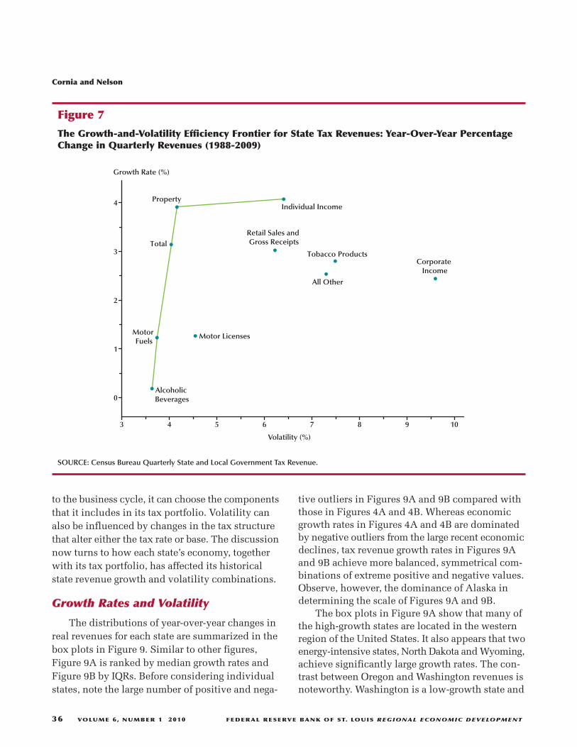
The Efficiency Frontier for IndividualState Taxes

Figure 7 plots the growth and volatility meas-ures for each tax category based on the mediangrowth rate and IQR for each category. Once again,the combination of low volatility and high growthis superior. Alcoholic beverages, motor fuels,property, and individual income exhibit this com-

bination and all lie on the efficiency frontier.Interestingly, the portfolio of total taxes would alsolie on the efficiency frontier. Individual incometax, as mentioned, has both high growth and highvolatility. This contrasts with the retail sales andgross receipts taxes, which have relatively lowergrowth and volatility. The inferiority of the com-bination of low growth and high volatility for thecorporate income tax is apparent by the tax’s farplacement from the efficiency frontier.

State Tax Portfolios

Figure 8 documents the diversity among statetax portfolios. Based on the fiscal 2008 total taxreceipts as reported by the Census Bureau, the figureshows proportions of revenue derived from eachpotential tax resource.

Cornia and Nelson


1 - Alcoholic Beverages

2 - Motor Fuels

8 - Total

9 - Property

7 - Retail Sales and Gross Receipts

5 - All Other

3 - Motor Licenses

10 - Individual Income

6 - Tobacco Products

4 - Corporate Income

–50 –30 –10 10 30 50

Percentage

Figure 6A

State and Local Taxes: Year-Over-Year Growth Rates in Quarterly Revenues Ranked by Median ofPercentage Change (1989-2009)

SOURCE: Census Bureau Quarterly State and Local Government Tax Revenue.

This figure highlights the importance of salesand income taxes at the state level, which individ-ually or together are significant components in allstate tax portfolios. Several states derive a substan-tial amount of revenue from the “All Other” cate-gory, including the energy-extraction states ofAlaska and Wyoming, as well as North Dakota,Delaware, Montana, and New Hampshire.

The ranking in Figure 8 is based on each state’sHerfindahl-Hirschman Index, which is calculated as

where si is the revenue share of the ith tax. NewHampshire, Montana, Vermont, and Delaware havebalanced portfolios. Alaska, Florida, South Dakota,Nevada, Washington, Texas, Tennessee, Hawaii,

H sii

N

==∑ 2

1,

and Oregon are largely dependent on a single taxsource and do not have diversified tax portfolios.

GROWTH AND VOLATILITY PATTERNS OF STATE TAX REVENUES

Thus far the empirical investigation reveals avariety of state economic reactions to differentphases of the business cycle. As discovered, uniquecharacteristics of each state’s economy stronglyinfluence the observed historical growth and volatil-ity combinations. Likewise, different types of taxesexhibit distinctive combinations of growth andvolatility.

Although each state has limited influence overthe economic structure that determines its reaction

Cornia and Nelson


1 - Alcoholic Beverages

2 - Motor Fuels

3 - Total

4 - Property

6 - Retail Sales and Gross Receipts

8 - All Other

5 - Motor Licenses

7 - Individual Income

9 - Tobacco Products

10 - Corporate Income

–50 –30 –10 10 30 50

Percentage

Figure 6B

State and Local Taxes: Year-Over-Year Growth Rates Ranked by IQR of Percentage Change (1989-2009)


to the business cycle, it can choose the componentsthat it includes in its tax portfolio. Volatility canalso be influenced by changes in the tax structurethat alter either the tax rate or base. The discussionnow turns to how each state’s economy, togetherwith its tax portfolio, has affected its historicalstate revenue growth and volatility combinations.

Growth Rates and Volatility

The distributions of year-over-year changes inreal revenues for each state are summarized in thebox plots in Figure 9. Similar to other figures,Figure 9A is ranked by median growth rates andFigure 9B by IQRs. Before considering individualstates, note the large number of positive and nega-

Cornia and Nelson


tive outliers in Figures 9A and 9B compared withthose in Figures 4A and 4B. Whereas economicgrowth rates in Figures 4A and 4B are dominatedby negative outliers from the large recent economicdeclines, tax revenue growth rates in Figures 9Aand 9B achieve more balanced, symmetrical com-binations of extreme positive and negative values.Observe, however, the dominance of Alaska indetermining the scale of Figures 9A and 9B.

The box plots in Figure 9A show that many ofthe high-growth states are located in the westernregion of the United States. It also appears that twoenergy-intensive states, North Dakota and Wyoming,achieve significantly large growth rates. The con-trast between Oregon and Washington revenues isnoteworthy. Washington is a low-growth state and

3 4 5 6 7 8 9 10

0

1

2

3

4

Tobacco Products

Property

Total

Alcoholic Beverages

Motor Fuels

Retail Sales and Gross Receipts

All Other

Motor Licenses

Individual Income

Corporate Income

Growth Rate (%)

Volatility (%)

Figure 7

The Growth-and-Volatility Efficiency Frontier for State Tax Revenues: Year-Over-Year PercentageChange in Quarterly Revenues (1988-2009)


Cornia and Nelson


Percentage

NHMTVTDEOKNM

MIWVNDKYUSNJPA

MNCAIL

LAAR

MDALKSIA

WIMEOHID

NCUTWYNERI

MOMA

INCONYSCVAGAAZCTMSORHITNTX

WANVSDFL

AK

0 20 40 60 80 100

Property

Sales

Individual Income

Corporate Income

Other

Figure 8

State Tax Portfolios: Proportions of Total 2008 Tax Revenues Ranked by the Herfindahl-HirschmanIndex

NOTE: Ranked from least to most diverse.

SOURCE: Census Bureau Annual State and Local Government Tax Revenue.

Cornia and Nelson


–100 0 100 200 300

Percentage

1 MI2 NM3 IA4 VT5 UT6 MT7 KY8 CT9 NE

10 AL11 MO12 WI13 HI14 OH15 WA16 MS17 WV18 DE19 KS20 NY21 SC22 NV23 ME24 OK25 RI26 SD27 PA28 MN29 IL30 TN31 NH32 US33 AZ34 LA35 NC36 FL37 AK38 IN39 MD40 OR41 MA42 GA43 TX44 VA45 NJ46 ID47 AR48 ND49 CA50 CO51 WY

Figure 9A

State Tax Revenues: Year-Over-Year Growth Rates in Quarterly Tax Receipts Ranked by Median ofPercentage Change (1995-2009)


Cornia and Nelson


1 US2 PA3 NC4 MO5 WA6 AL7 TN8 NE9 MA

10 IL11 SD12 KS13 NY14 TX15 AR16 WI17 IN18 CA19 RI20 WV21 AZ22 CO23 OK24 KY25 GA26 FL27 DE28 ME29 HI30 IA31 CT32 VT33 LA34 OH35 MN36 SC37 MS38 NH39 MD40 NJ41 VA42 MT43 OR44 ID45 ND46 UT47 MI48 NV49 NM50 WY51 AK

–100 0 100 200 300

Percentage

Figure 9B

State Tax Revenues: Year-Over-Year Growth Rates in Quarterly Tax Receipts Ranked by IQR ofPercentage Change (1995-2009)


depends heavily on the sales tax. Oregon, its neigh-bor, is a high-growth state because it depends onthe individual income tax. Thus we see that taxstructure might strongly influence the growth rate.

Figure 9B ranks states by the volatility of theirtax revenues as measured by the IQR and showsthat the western states with high growth rates alsohave high levels of variability. This is especiallytrue for Alaska and Wyoming. Interestingly, Texasis not as volatile. As expected because of diversity,the U.S. aggregate of total state revenues is not veryvolatile. The highly stable tax receipts of Tennesseeare probably influenced by its dependence on theretail sales tax rather than the individual incometax.

The Efficiency Frontier for State Revenues

Figure 10 plots the growth and volatility ofstate tax revenue based on the medians in 9A andIRQs in Figure 9B, respectively. The line in Figure 10identifies those states with efficient combinations.As mentioned, Wyoming has both a high growthrate and high volatility and finds itself on the effi-ciency frontier. Colorado, California, Arkansas, andTexas seem to achieve relatively higher growthrates without incurring significantly more volatility.Other states that distinguish themselves by beingon the efficiency frontier are Massachusetts andNorth Carolina. This raises an interesting futureresearch question about the combinations of eco-nomic and tax structure characteristics that generate

Cornia and Nelson


–4

0

4

8

WY

AK

CO

CAARTX

MANCUS

MI

UT

NV

IA

NM

0 10 20 30 40 50

Growth Rate (%)

Volatility (%)

Figure 10

The Growth-and-Volatility Efficiency Frontier for State Tax Revenues: Year-Over-Year PercentageChange in Quarterly Total State Tax Receipts (1995-2009)


tax revenues with desirable growth and volatilityattributes.

AD HOC OBSERVATIONS OFINDIVIDUAL STATES

Ad hoc comparisons give some insight intotax policies that can exacerbate or moderate astate’s dependence on the business cycle. Theycan also highlight potential practices that mightmoderate the adverse effect of low-growth and/orhighly volatile state economies on tax revenues.

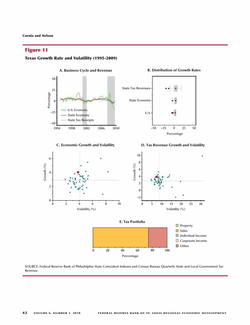
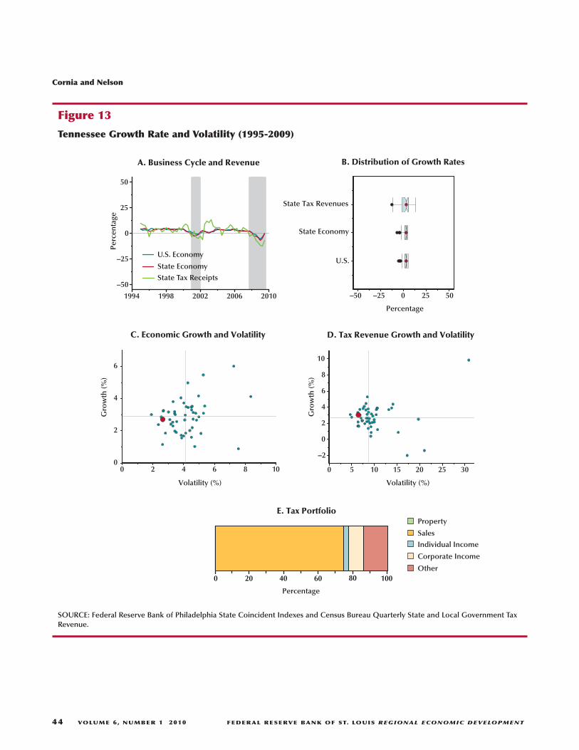
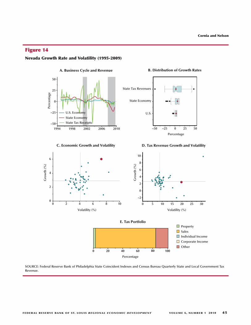
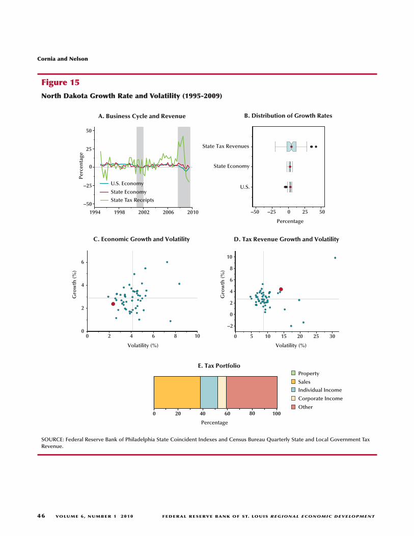
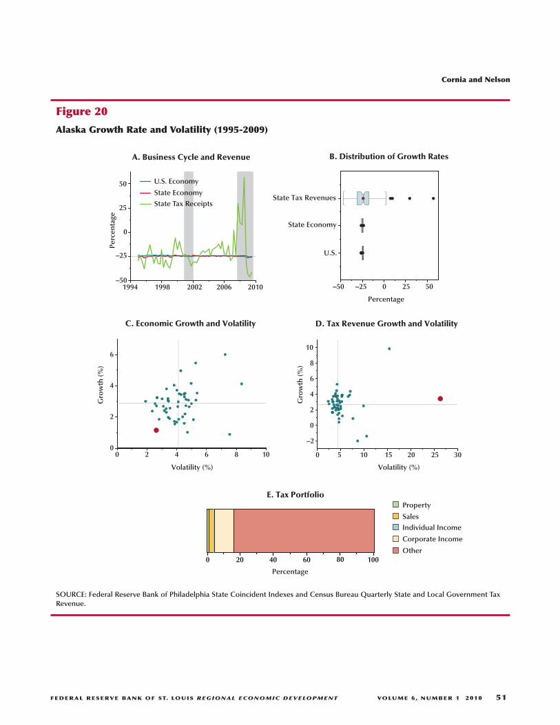
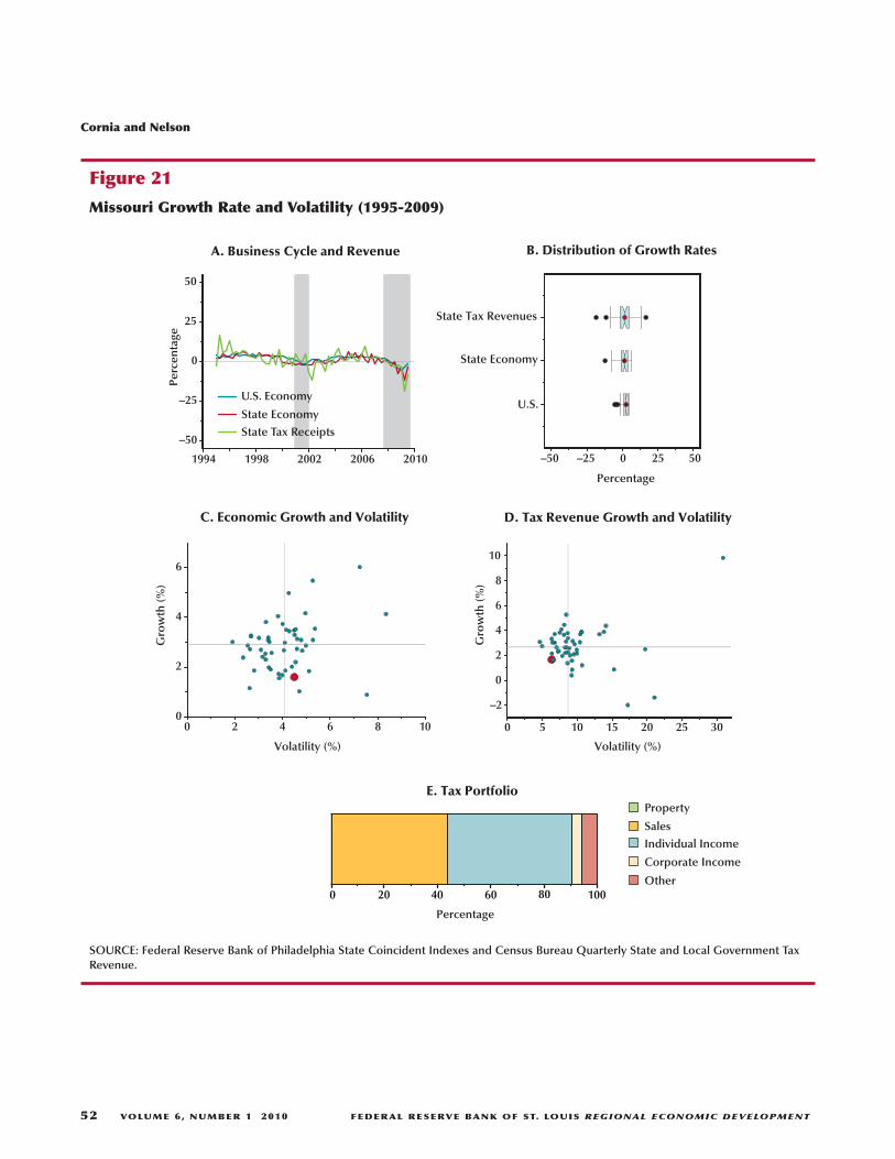
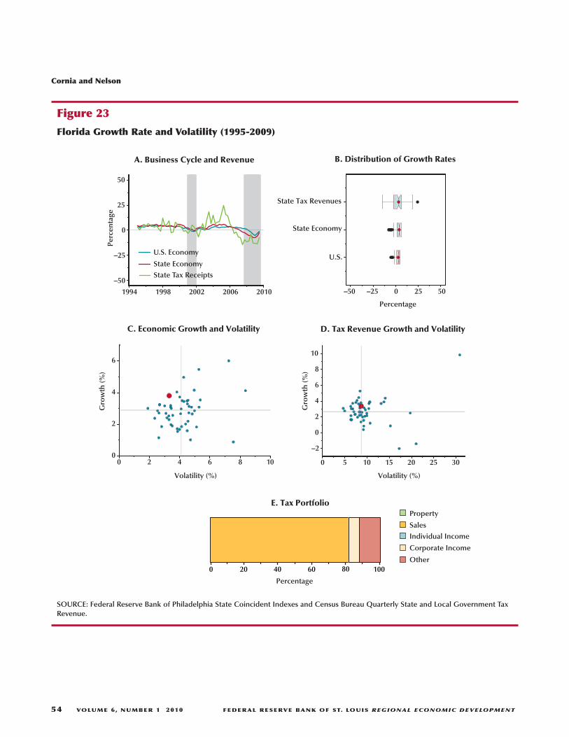
In Figures 11 to 23, summary diagrams forselected states offer insight into best practices.Panel A compares the growth rates of the givenstate’s tax receipts (green), its economy (red), andthe national economy (blue). The box plots inPanel B compare the distributions of the rates ofchange for these same three categories. The scatterplots in Panels C and D show how the given state’sgrowth and volatility compared with the growthand volatility of all other individual state economiesand tax structures, respectively. Panel E shows thecomposition and balance of the given state’s taxportfolio.

First, consider Texas (Figure 11), which dis-tinguishes itself by having both its economy andtax revenues on the efficiency frontier. Both exhibitmedium growth and volatility (Panels C and D,respectively). Its economy closely follows thenational pattern, which is evident in the time-seriesgraph (Panel A) and the box plots (Panel B). Its taxportfolio depends primarily on the sales tax; how-ever, “other” revenues also contribute significantlyto total state revenues (Panel E). This tax portfolioplaces Texas’s revenues in the moderate-growthand moderate-volatility category (Panel D).

Neither the Arkansas (Figure 12) nor Tennessee(Figure 13) economies reach the efficiency fron-tier (Panels C), but their tax portfolios give themimproved combinations of growth and volatilitythat put their tax revenues on the efficiency frontier(Panels D, respectively). Both economies closelymimic the national growth pattern (Panels A).Interestingly, their tax portfolios differ (Panels E):Arkansas depends on a combination of property,sales, individual income, corporate income, and

“other” tax categories. This combination keepsArkansas’s tax revenues from being placed with itseconomy in the low-growth/low-volatility quad-rant, by supporting a higher relative growth ratewithout adding too much additional volatility.Tennessee depends primarily on the sales tax.

For Nevada (Figure 14), a high growth rate andhigh volatility place its economy on the efficiencyfrontier (Panel C). Nevada’s dependence on thesales tax without any income tax (Panel E) signifi-cantly hinders the growth rate of its tax revenuesbut, surprisingly, does not commensurately decreaseits volatility. The result is an inferior combinationof low growth and high volatility (Panel D).

North Dakota (Figure 15) has a tax portfoliothat generates higher growth and volatility relativeto other states (Panel E). Its economy does not fol-low the national pattern as closely as the previouslydiscussed states. Sometimes its growth rate exceedsthat of the national business cycle and sometimesit is lower. North Dakota does not seem to haveexperienced the extreme declines that occurred inmany other states during the Great Recession. NorthDakota’s tax portfolio is balanced and depends onsales, individual income, and “other” taxes.

The macroeconomic challenges in Michigan(Table 16) strongly influence its tax revenue. Asmentioned, it is the only state with negative aver-age economic growth. The low economic growthand corresponding high volatility (Panel C) havecreated severe fiscal challenges. Even thoughMichigan has a balanced dependence on salesand income taxes (Panel E), its tax system seemsto exacerbate the revenue challenges, as its taxrevenues remain in the unfavorable low-growth/high-volatility quadrant (Panel D).

As mentioned, Washington and Oregon(Figures 17 and 18) provide an interesting compari-son in tax policy. They have similar economiesthat are more volatile than the national economybut that also have higher expected growth ratesthan other state economies. Oregon’s economy isslightly more volatile than Washington’s. This dis-similarity lies mostly in each state’s reliance onone major tax. Oregon depends primarily on theindividual income tax, Washington on the retailsales tax (Panels E, respectively). The growth andvolatility of each state’s tax revenue shows the

Cornia and Nelson


Cornia and Nelson


Percentage

1994 1998 2002 2006 2010

–50

–25

0

25

50

Perc

enta

ge

A. Business Cycle and Revenue

–50 –25 0 25 50

Percentage

U.S.

State Economy

State Tax Revenues

0 2 4 6 8 100

2

4

6

Gro

wth

(%)

0 5 10 15 20 25 30

–2

0

2

4

6

8

10

Gro

wth

(%)

B. Distribution of Growth Rates

C. Economic Growth and Volatility D. Tax Revenue Growth and Volatility

E. Tax PortfolioProperty

Sales

Individual Income

Corporate Income

Other

U.S. Economy

State Economy

State Tax Receipts

0 20 40 60 80 100

Volatility (%) Volatility (%)

Figure 11

Texas Growth Rate and Volatility (1995-2009)


Cornia and Nelson


Property

Sales

Individual Income

Corporate Income

Other

U.S. Economy

State Economy

State Tax Receipts

Percentage

1994 1998 2002 2006 2010

–50

–25

0

25

50

Perc

enta

ge


–50 –25 0 25 50

Percentage

U.S.

State Economy

State Tax Revenues

0 2 4 6 8 100

2

4

6

Gro

wth

(%)

0 5 10 15 20 25 30

–2

0

2

4

6

8

10

Gro

wth

(%)



E. Tax Portfolio

0 20 40 60 80 100


Figure 12

Arkansas Growth Rate and Volatility (1995-2009)


Cornia and Nelson


Property

Sales

Individual Income

Corporate Income

Other

U.S. Economy

State Economy

State Tax Receipts

Percentage

1994 1998 2002 2006 2010

–50

–25

0

25

50

Perc

enta

ge


–50 –25 0 25 50

Percentage

U.S.

State Economy

State Tax Revenues

0 2 4 6 8 100

2

4

6

Gro

wth

(%)

0 5 10 15 20 25 30

–2

0

2

4

6

8

10

Gro

wth

(%)



E. Tax Portfolio

0 20 40 60 80 100


Figure 13

Tennessee Growth Rate and Volatility (1995-2009)


Cornia and Nelson


Property

Sales

Individual Income

Corporate Income

Other

U.S. Economy

State Economy

State Tax Receipts

Percentage

1994 1998 2002 2006 2010

–50

–25

0

25

50

Perc

enta

ge


–50 –25 0 25 50

Percentage

U.S.

State Economy

State Tax Revenues

0 2 4 6 8 100

2

4

6

Gro

wth

(%)

0 5 10 15 20 25 30

–2

0

2

4

6

8

10

Gro

wth

(%)



E. Tax Portfolio

0 20 40 60 80 100


Figure 14

Nevada Growth Rate and Volatility (1995-2009)


Cornia and Nelson


Property

Sales

Individual Income

Corporate Income

Other

U.S. Economy

State Economy

State Tax Receipts

Percentage

1994 1998 2002 2006 2010

–50

–25

0

25

50

Perc

enta

ge


–50 –25 0 25 50

Percentage

U.S.

State Economy

State Tax Revenues

0 2 4 6 8 100

2

4

6

Gro

wth

(%)

0 5 10 15 20 25 30

–2

0

2

4

6

8

10

Gro

wth

(%)



E. Tax Portfolio

0 20 40 60 80 100


Figure 15

North Dakota Growth Rate and Volatility (1995-2009)


Cornia and Nelson


Property

Sales

Individual Income

Corporate Income

Other

U.S. Economy

State Economy

State Tax Receipts

Percentage

1994 1998 2002 2006 2010

–50

–25

0

25

50

Perc

enta

ge


–50 –25 0 25 50

Percentage

U.S.

State Economy

State Tax Revenues

0 2 4 6 8 100

2

4

6

Gro

wth

(%)

0 5 10 15 20 25 30

–2

0

2

4

6

8

10

Gro

wth

(%)



E. Tax Portfolio

0 20 40 60 80 100


Figure 16

Michigan Growth Rate and Volatility (1995-2009)


Cornia and Nelson


Property

Sales

Individual Income

Corporate Income

Other

U.S. Economy

State Economy

State Tax Receipts

Percentage

1994 1998 2002 2006 2010

–50

–25

0

25

50

Perc

enta

ge


–50 –25 0 25 50

Percentage

U.S.

State Economy

State Tax Revenues

0 2 4 6 8 100

2

4

6

Gro

wth

(%)

0 5 10 15 20 25 30

–2

0

2

4

6

8

10

Gro

wth

(%)



E. Tax Portfolio

0 20 40 60 80 100


Figure 17

Washington Growth Rate and Volatility (1995-2009)


Cornia and Nelson


Property

Sales

Individual Income

Corporate Income

Other

U.S. Economy

State Economy

State Tax Receipts

Percentage

1994 1998 2002 2006 2010

–50

–25

0

25

50

Perc

enta

ge


–50 –25 0 25 50

Percentage

U.S.

State Economy

State Tax Revenues

0 2 4 6 8 100

2

4

6

Gro

wth

(%)

0 5 10 15 20 25 30

–2

0

2

4

6

8

10

Gro

wth

(%)



E. Tax Portfolio

0 20 40 60 80 100


Figure 18

Oregon Growth Rate and Volatility (1995-2009)


Cornia and Nelson


Property

Sales

Individual Income

Corporate Income

Other

U.S. Economy

State Economy

State Tax Receipts

Percentage

1994 1998 2002 2006 2010

–50

–25

0

25

50

Perc

enta

ge


–50 –25 0 25 50

Percentage

U.S.

State Economy

State Tax Revenues

0 2 4 6 8 100

2

4

6

Gro

wth

(%)

0 5 10 15 20 25 30

–2

0

2

4

6

8

10

Gro

wth

(%)



E. Tax Portfolio

0 20 40 60 80 100


Figure 19

California Growth Rate and Volatility (1995-2009)


Cornia and Nelson


Property

Sales

Individual Income

Corporate Income

Other

U.S. Economy

State Economy

State Tax Receipts

Percentage

1994 1998 2002 2006 2010–50

–25

0

25

50

Perc

enta

ge


–50 –25 0 25 50

Percentage

U.S.

State Economy

State Tax Revenues

0 2 4 6 8 100

2

4

6

Gro

wth

(%)

0 5 10 15 20 25 30

–2

0

2

4

6

8

10

Gro

wth

(%)



E. Tax Portfolio

0 20 40 60 80 100


Figure 20

Alaska Growth Rate and Volatility (1995-2009)


Cornia and Nelson


Property

Sales

Individual Income

Corporate Income

Other

U.S. Economy

State Economy

State Tax Receipts

Percentage

1994 1998 2002 2006 2010

–50

–25

0

25

50

Perc

enta

ge


–50 –25 0 25 50

Percentage

U.S.

State Economy

State Tax Revenues

0 2 4 6 8 100

2

4

6

Gro

wth

(%)

0 5 10 15 20 25 30

–2

0

2

4

6

8

10

Gro

wth

(%)



E. Tax Portfolio

0 20 40 60 80 100


Figure 21

Missouri Growth Rate and Volatility (1995-2009)


Cornia and Nelson


Property

Sales

Individual Income

Corporate Income

Other

U.S. Economy

State Economy

State Tax Receipts

Percentage

1994 1998 2002 2006 2010

–50

–25

0

25

50

Perc

enta

ge


–50 –25 0 25 50

Percentage

U.S.

State Economy

State Tax Revenues

0 2 4 6 8 100

2

4

6

Gro

wth

(%)

0 5 10 15 20 25 30

–2

0

2

4

6

8

10

Gro

wth

(%)



E. Tax Portfolio

0 20 40 60 80 100


Figure 22

Illinois Growth Rate and Volatility (1995-2009)


Cornia and Nelson


Property

Sales

Individual Income

Corporate Income

Other

U.S. Economy

State Economy

State Tax Receipts

Percentage

1994 1998 2002 2006 2010

–50

–25

0

25

50

Perc

enta

ge


–50 –25 0 25 50

Percentage

U.S.

State Economy

State Tax Revenues

0 2 4 6 8 100

2

4

6

Gro

wth

(%)

0 5 10 15 20 25 30

–2

0

2

4

6

8

10

Gro

wth

(%)



E. Tax Portfolio

0 20 40 60 80 100


Figure 23

Florida Growth Rate and Volatility (1995-2009)


varying effects of these choices. Washington’sdependence on the sales tax places its tax revenuesin the low-growth/low-volatility quadrant (Figure 17,Panel D). Oregon’s dependence on the income taxkeeps its tax revenues far from the efficiency fron-tier by maintaining or increasing the undesirablecombination of lower expected growth for the givenlevel of volatility.

Interestingly, California (Figure 19) exhibitsno extremes in growth and volatility for either itseconomy or tax revenues. It might be, therefore, thatthe well-documented fiscal travails of Californiaare more strongly related to its budgeting andlegislative process than to inherent tax structuredeficiencies or economic instability.

Alaska (Figure 20) is an example of the extremepotential effects on growth and volatility that canbe exerted by a tax portfolio. Because of the widefluctuations in the rates of change shown in PanelA, it is difficult to evaluate Alaska’s economy rela-tive to the U.S. economy. The panel does show,however, the dominance of revenue volatility rel-ative to the economy. Alaska’s choice to dependon “other” and corporate income taxes rather thansales or individual income taxes causes its taxrevenues to have particularly high expected growthand volatility.

The additional examples in Figures 21 through23 further demonstrate the potential positive andnegative effects of tax policy. Although Missouri’seconomy sits in the low-growth/high-volatilityquadrant (Figure 21, Panel C), its tax portfoliosuccessfully places its tax revenues in the more-desirable low-growth/low-volatility quadrant(Panel D). Illinois’s economy sits in the inferiorlow-growth/high-volatility quadrant (Figure 22,Panel C), and it tax revenues in the high-growth/low-volatility quadrant (Panel D). Finally, althoughFlorida’s economy sits on the efficiency frontier(Figure 23, Panel C), its tax code keeps its tax rev-enues off the efficiency frontier by decreasing theirgrowth and increasing their volatility relative tothose measures for other states (Panel D).

BUDGETING IMPLICATIONSAs mentioned, revenue adequacy is a key cri-

terion used to evaluate tax systems. Because electedofficials rarely have the political ability to simply

stop funding services such as education or publicsafety, they need reliable revenue sources. For thisreason, good public policy suggests that states workto mitigate revenue uncertainty. While recognizingthe importance of equity and efficiency in tax pol-icy formulation, even the best-intended tax designcannot offset the instability resulting from taxschemes that magnify rather than attenuate busi-ness cycle effects.

Super (2005) notes that economists’ growingsophistication in understanding business cyclesshould translate into better prediction of fiscalcycles. Given the severity of the current downturn,however, his observations may be slightly prema-ture and overly optimistic. Nonetheless, under-standing the fiscal consequences of downturns mayhelp develop policies that allow rational responsesto fiscal trauma. Two examples of methods thatincorporate growth and volatility into budgetingdecisions are revenue semaphores and value at risk(VAR). Neither method has anything to do withreforming tax systems to make them more stable.They simply show that information about growthand volatility can improve state policy processesand budget outcomes.

Revenue Semaphores

Revenue semaphores (Cornia, Nelson, andWilko, 2004) aid the budgeting process by provid-ing a graphical approach for communicatingexpected growth and volatility of each potentialrevenue source so that expenditures may be prior-itized. Rather than provide a single-valued pointforecast of tax revenues, revenue semaphores cat-egorize the distribution of potential tax receipts intothree different categories. As shown in Figure 24,the first, green for “go,” identifies those revenuesavailable for basic expenditures. Although a smallprobability always exists for a major economicupheaval, these revenues can usually be consideredsafe parts of base budgets. The second category,yellow for “caution,” includes highly likely rev-enues, which are allocated to projects and expen-ditures likely to be fully funded. With thiscategorization, in the case of revenue shortfalls,state executive and legislative branches can moreeasily see where they need to cut back to balancethe budget. The third category, red for “stop,”

Cornia and Nelson


identifies potential—although unlikely—revenuesthat could allow capital expenditures or tax cutsin the case of a very large revenue surplus. Eventhough “red revenues” are highly unlikely, antici-pating these potential windfall resources couldfoster more transparent decisionmaking at the endof the budget year.

Implementation of revenue semaphores requiresthat analysts and officials consider the growthand volatility of their state economies. They mustalso consider the potential impact on growth andvolatility that comes from their chosen tax portfolio.These factors, as they interact to determine avail-able revenues in the budgeting process, determinethe boundaries for the green, yellow, and red cate-gories of revenue semaphores.

Value at Risk and Optimal Rainy DayFunds

Nelson and Cornia (2004) use the financial con-cept of VAR to show how states should consider

the entire probability distribution of budget sur-pluses/deficits when determining the optimal sizeof their rainy day funds. Probability distributionssimilar to the one shown in Figure 25 are criticalfor the application of VAR methodology to rainyday funds.

If one considers state rainy day funds as a typeof insurance, it is reasonable to recognize that it isinfeasible to totally insure against all adverse andimprobable outcomes. The size of a rainy day fundneeded to cover the worst-possible budget deficitwould be neither politically possible nor financiallyfeasible. Therefore, when determining the optimalsize of a rainy day fund, decisionmakers mustdecide how large of a budget deficit can be insured.Using VAR, decisionmakers simply determine theprobability, p, of the deficit size they cannot insure.The dollar amount that leaves a probability of p inthe left tail of the probability distribution, like theone shown in Figure 25, corresponds to the VAR.This value then determines the size of the rainyday fund.

The expected growth and volatility of tax rev-enues strongly impacts the probability distributionof deficits/surpluses, such as the one in Figure 25.For this reason, states should carefully considerthe unique characteristics of their economy andtax portfolio when calculating the optimal size oftheir rainy day funds. The application of a simplerule of thumb without customization to a state’seconomic and tax environment will result in asuboptimal solution.

SUMMARY, CONCLUSION, ANDRECOMMENDATIONS

This analysis establishes the joint importanceof economic conditions and tax portfolios in deter-mining the growth and volatility of state tax rev-enues. It also reveals that a variety of growth andvolatility combinations exist among states. Asstates consider tax reform and revenue-enhancingmeasures in the current fiscal crisis, they shouldcarefully anticipate and consider the possibleimpacts of their proposed changes on the growthand volatility of their unique tax revenue portfolios.

Cornia and Nelson


Green Range:Generally Dependable

Revenues

BaseBudget

Yellow Range:Highly Likely

Revenues

FlexibleSpending

Red Range: Potential,

Though Unlikely, Revenues

DreamProjectsRED

YELLOW

GREEN

Figure 24

Revenue Semaphores

The current recession has wrought budgetinghavoc among states. The Philadelphia Fed’s coin-cident indexes clearly establish the historic gravityof the most recent economic downturn. Althoughsome states have been more severely affected thanothers, all states have suffered challenges due tothe economic slowdown. Because state economiesdo not react uniformly to the national businesscycle, state officials must take care that they tailorpolicy proposals to the unique characteristics oftheir economy.

In the short run, states cannot alter the volatil-ity of their economies, but they can change theirtax portfolios to minimize the effects of the businesscycle on their fiscal health. For this reason theyneed to consider the natural tendencies of theireconomies when formulating tax policy. Thismeans that states with volatile economies mightwant to choose tax portfolios that minimize theimpact of national macroeconomic trends and

avoid volatile funding sources that can result ineven more volatile revenues. States with stableeconomies might consider adopting more aggres-sive tax portfolios.

This analysis recognizes the importance ofsales and individual income taxes as the principalrevenue sources in state budgeting. The sales taxoffers stability but at the cost of a lower growthrate. The individual income tax offers growth butat the cost of increased volatility. Although theproperty tax currently is used mostly for financinglocal governments, its attractive growth and volatil-ity combination might mean that states shouldconsider adopting it as an additional source offunding to complement the growth and volatilitycharacteristics of the sales and individual incometaxes.

More research is needed to understand how astate’s economy and tax portfolios interact to deter-mine the growth and volatility of its tax revenues.

Cornia and Nelson


Budget Surplus or Deficit

Probability of Inadequate Rainy Day Funds

5%

Probability of Surplus

57%

Optimal VAR Rainy Day Funds

Probability

Figure 25

Optimal Rainy Day Funds Determined as Value at Risk

Better understanding of the probabilistic charac-teristics of tax revenues will improve the budgetingprocess in ways beyond the revenue semaphoresand optimal rainy day funds discussed in thispaper. Formal econometric modeling can exploit

the panel nature of the economic and revenuedata to formalize the ad hoc findings presented inthis paper. The resulting knowledge could signifi-cantly improve tax reform and budget-balancingpublic policy decisions.

Cornia and Nelson


REFERENCESCornia, Gary C.; Nelson, Ray D. and Wilko, Andrea. “Fiscal Planning, Budgeting, and Rebudgeting Using Revenue

Semaphores.” Public Administration Review, March 2004, 64(2), pp. 164-79.

Crain, W. Mark. Volatile States: Institutions, Policy, and the Performance of American State Economies. Ann Arbor,University of Michigan Press, 2003.

Crone, Theodore M. and Clayton-Matthews, Alan. “Consistent Economic Indexes for the 50 States.” Review ofEconomics and Statistic, November 2005, 87(4), pp. 593-603.

Dadayan, Lucy and Boyd, Donald J. “State Tax Revenues Show Record Drop, for Second Consecutive Quarter.”Nelson A. Rockefeller Institute of Government State Revenue Report, October 2009, No. 77, pp. 1-23.

Gamage, David S. “Preventing State Budget Crises: Redefining ‘Tax Cuts’ and ‘Tax Hikes.’” California Law Review(forthcoming).

Groves, Harold M. and Kahn, Harry C. “The Stability of State and Local Tax Yields.” American Economic Review,March 1952, 42(1), pp. 87-102.

Holcombe, Randall G. and Sobel, Russell S. Growth and Variability in State Tax Revenue: An Anatomy of StateFiscal Crises. Westport, CT: Greenwood Press, 1987.

Nelson, Ray D. and Cornia, Gary C. “Rainy Day Funds and Value at Risk.” Tax Analysts State Tax Notes, August 25,2003, 29(8), pp. 563-67.

Sobel, Robert S. and Wagner, Gary C. “Cyclical Variability in State Government Revenue: Can Tax Reform ReduceIt?” Tax Analysts State Tax Notes, August 25, 2003, 29(8), pp. 569-76.

Stock, James H. and Watson, Mark W. “New Indexes of Coincident and Leading Economic Indicators,” in O.J.Blanchard and S. Fischer, eds., NBER Macroeconomics Annual 1989. Cambridge, MA: MIT Press, 1989, pp. 351-94.

Super, David A. “Rethinking Fiscal Federalism.” Harvard Law Review, June 2005, 118(8), pp. 2546-652.

Tufte, Edward R. The Visual Display of Quantitative Information. Second Ed. Cheshire, CT: Graphics Press, 2001.

Tukey, John W. Exploratory Data Analysis. Reading, MA: Addison-Wesley, 1977.

State Tax Revenue Growth and Volatility · State Tax Revenue Growth and Volatility Gary C. Cornia...

Documents

Transcript of State Tax Revenue Growth and Volatility · State Tax Revenue Growth and Volatility Gary C. Cornia...