State presentation2
53
Group C MBM 1 st Semester NCC Descriptive Analysis
-
Upload
lata-bhatta -
Category
Education
-
view
128 -
download
1
Transcript of State presentation2

Group C
MBM 1st Semester
NCC
Descriptive Analysis

• Measure of Central Tendency• Measure of dispersion• Skewness & kurtosis.• Five number summary• Box- Whisker plot
Agendas

Measures of Central Tendency
Introduction Single Data Represents a set of
Data
Concentrates towards the middle of the
distribution.

• Mean or Average Simply Mean is the sum of all the observations divided by
the number of observation (A.M, G.M, H.M, C.M,W.M)
• Median Median is the positional average of the given series of n
observation arranged in an ascending or descending order
of magnitude
• Mode The variate value that occurs most frequently is known as
a mode. It is denoted by Mo
Various Measures of Central Tendency

Arithmetic Mean ( or simply mean)
Individual Series
Direct Method
X̅ = n = No. of observation∑X = Sum of all observation
Short Cut Method X̅ = (a + Σd)/n a= assumed mean, d=
deviation from assumed
mean = X-a
n = total number of
observation

Discrete Series
Direct Method X̅ = Σfx/N
Short cut method ̅X̅= a+ Σfd/N

• Continuous Series: The formula for continuous
series is the same as for discrete series, the only
difference is that the middle value of a class is to
be taken as X in case of continuous series.

• Observation of the central of data set• Suitable when the average of qualitative• Appropriate for the open ended classified data.
Median

Method of calculation
series
Individual Series
•Ascending or Descending order
Md= value of (n+1/2) th item
Discrete Series • Calculation of c.f
Md= (n+1)/2
ContinuousSeries
•Class should be exclusive
Md=n/2
Md=L+(n/2 -cf)/F*h

• Dictionary meaning “ most used”• Value that occurs more often or with the greatest
frequency
Mode

Type of Series
Individual the value which has
maximum repetition.
Discrete value of variate which has
maximum frequency is the
mode.
Continuous
Mode

Central tendency measures do not reveal
the variability present in the data.
Dispersion is the scatteredness of the data
series around it average.
Dispersion is the extent to which values
in a distribution differ from the average
of the distribution.
What is measures of dispersion?

Determine the reliability of an average Serve as a basis for the control of the
variability To compare the variability of two or more
series and Facilitate the use of other statistical measures.
Why we need measures of dispersion?
(Significance)

1. Range
2. Quartile Deviation
3. Mean Deviation
4. Standard Deviation
These are called absolute measures of dispersion
Absolute measures have the units in which the
data are collected.
Method of Measuring Dispersion

• RangeThe range is the simplest possible measure of dispersion and is defined as the difference between the largest and smallest values of the variable.
In symbols,Range = L – S.
Where, L = Largest value.S = Smallest value.
Usually used in combination with other measures of dispersion.

The important relative measures of dispersion are• Coefficient of Range • Coefficient of Quartile Deviation• Coefficient of Mean Deviation• Coefficient of Standard Deviation
Relative measure of dispersion is the ratio of a
measure of dispersion to an appropriate average
from which deviations were measured.

• In individual observations and discrete series, L and Sare easily identified. In continuous series, the following
two methods are followed:Method 1:L = Upper boundary of the highest classS = Lower boundary of the lowest class.Method 2:L = Mid value of the highest class.S = Mid value of the lowest class.
Coefficient of Range :• Range is an absolute value, so it cannot compare two
distribution with different units.• For the comparison of such distribution coefficient of
range is used. • In Symbol , Coefficient of Range= (L-S) / (L+S)

• Quartile Deviation
Quartile Deviation is half of the difference between the first and
third quartiles. Hence, it is called Semi Inter Quartile Range.
In Symbols, among the quartiles Q1, Q2 and Q3, the range Q3-
Q1 is called inter quartile range and (Q1-Q3)/2 is quartile
deviation or semi inter quartile range.
Coefficient of Quartile Deviation : The relative measure based on
lower and upper quartile is known as coefficient of Q.D.
Q.D= (Q3-Q1)/(Q3+Q1)

Mean Deviation
Measures the ‘average’ distance of each observation away
from the mean of the data .
Deviation from A.M, Median and Mode
Generally more sensitive than the range or interquartile range,
since a change in any value will affect it.

• Formula for calculating Mean Deviation
~ Mean Deviation from Mean = Σf|x - X̅ |/n~ Mean Deviation from Median = Σf | X- median|/n~ mean Deviation from Mode = Σf | X- mode|/n
Note: Frequency (f) does not mention in individual series.

Standard Deviation
• Standard Deviation is Standard Deviation
• Positive square of the arithmetic mean of the square of
the deviation taken from the A.M.
• The most common and best measure of dispersion
• Takes into account every observation

Basic Formula of standard Deviation
SD ( ϭ) = Σ(x-x )2
N
• The square of standard deviation is called the
variance.

Coefficient of variation
– Compare the variability between two set of data
– expressed as a percentage rather than in terms of the units
of the particular data
Formula for coefficient of variation (CV):
CV = ϭ / X̅ * 100

Skewness
• Lack of Symmetry.
• According to distribution of data, Skewness is
used to measure the shape drawn from
frequency distribution.
• Relates to the shape of the curve.

For example
set A set B
variable (X) frequency (f) variable (X) frequency (f)
10 5 10 5
15 15 15 20
20 30 20 15
25 30 25 45
30 15 30 10
35 5 35 5
Total 100 100

• In set A & B of the above Example both have same mean , x=
22.5 or standard deviation =6.02 the curve drawn for both
cases shows that they have different shapes. Following are the
shape of the curve for set A & Set B.
The curve of set A is non skewed or normal curve.

The curve of Set BThe shape of the frequency distribution is skewed .

When?????If…..
• Arithmetic mean≠ median≠ mode• Quartiles are not equi -distant from the median• The curve drawn from the frequency distribution
isn't of bell shape type.
A distribution of data said to be skewed

Types of Skewness
According to the view of elongation of the tail of the curve of the
frequency distribution are as follow.
• No Skewness or symmetry
• Positive Skewness
• Negative Skewness

No Skewness
• Distribution of the data said to be no skewed if the curve
drawn from the data is Neither elongated more to the left nor
to the right side.
• The curve equally elongated to the right as well as to the left
side
• if Mean= median= mode

Positive Skewness
• A distribution of the data is said to have positive skewness or
right skewed if the curve drawn from the data is more
Elongated to the right side
• Mean Median Mode

Negative Skewness
• A distribution of data is said to have negative Skewness of left
skewed if the curve drawn from the data is more elongated to
the left side
• Mean Median Mode


• Absolute Measure :- It express in terms of original units of the data so it is not appropriate.
• Relative measure:- It relates with the consistency it doesn’t contain any units of the data.
Measures of Skewness

Relative methods of measuring
Skewness
• Karl Pearson’s measure of Skewness
• Bowley’s measure of Skewness
• Kelly’s measure of Skewness

Pearson’s measure of Skewness
Absolute measure of Skewness not in widely used , expressed in
the terms of original unit of data .
a) Skewness= mean- mode
b) Skewness= mean- median
The relative measure of Skewness is coefficient of Skewness &
frequently used.
If mode is defined: Sk= mean- mode / S.D.
If mode is ill defined: Sk = 3(mean- median)/ S.D.
Pearson’s coefficient of Skewness generally lies between -3 &+3.

Bowley's measure of Skewness
• Absolute measure of Skewness is
Skewness= Q3+Q1- 2Md
• Also known as quartile measure of Skewness
• Lies between -1 & +1
• It is used when, Open ended classes having ill defined mode &
distribution with extreme observation & particularly useful .
Sk(B)= Q3+Q1-2 Md/ Q3-Q1

Interpretation of results of Pearson’s measures:-
• If Sk(P)= 0 distribution is symmetrical ( non-
skewed)
• If Sk(P)>0 distribution is positively skewed.
• If Sk(P)<0 distribution is negatively skewed.
Interpretation of results of Bowley’s measures:-
• Sk(B)= 0, distribution is symmetrical.
• Sk (B)>0, distribution is positively skewed.
• Sk(B)<0, distribution is negatively skewed.

Kelly’s measure of Skewness
Kelly’s absolute measure of Skewness
• Skewness= P90+P10-2P50
• Skewness= D9+D1-2D5
Kelly’s Coefficient of Skewness is
• Sk (Kelly)= P90+P10-2P50/P90-P10
• Sk (Kelly)= D9+D1-2D5/D9-D1
• Percentile measure of Skewness
• Seldom used in practice.

• Besides central tendency, dispersion and skewness, kurtosis is the also one of the measure by which the frequency distribution can be described and compared.
• The study of kurtosis helps in studying the peakedness of the frequency distribution in comparison to normal distribution.
• Measure of kurtosis give the extent to which the distribution is more peaked or flat topped with respect to the normal curve.
Kurtosis

Types of kurtosis
• Mesokurtic• Leptokurtic• Platykurtic

Measures of kurtosis
• Kurtosis can be measured with the help of quartiles and
percentiles.
• Measures of kurtosis based on quartiles and percentiles is
known as percentile coefficient of kurtosis.
• It is denoted by k and calculated as:
k=1/2(Q3-Q1)/P90-P10
where Q3=upper quartile P90=90th percentile
Q1=lower quartile P10=10th percentile
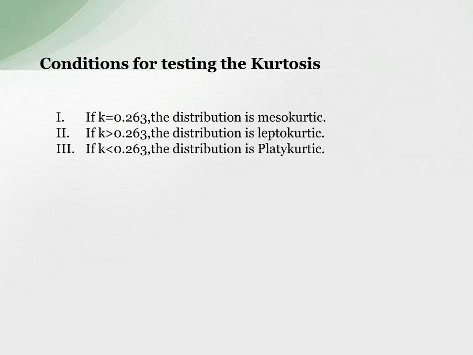
Conditions for testing the Kurtosis
I. If k=0.263,the distribution is mesokurtic.II. If k>0.263,the distribution is leptokurtic.III. If k<0.263,the distribution is Platykurtic.

• Five point summary is the descriptive tool• Provide information about the set of observation• The five-number summary provides a concise
summary of the distribution of the observations.
• It allow to recognize the shape of data set.
Five point summary

• It consist of 5 important items:
–the sample minimum (smallest observation)
– the lower quartile or first quartile– the median (middle value)–the upper quartile or third quartile –the sample maximum (largest
observation)

• five-number summary gives information about– the location (from the median), – spread (from the quartiles) and – range (from the sample minimum and maximum) of
the observations

• Shows how the data is distributed using the following components– Median– Upper quartiles– Lower quartiles– Maximum and Minimum Values
Box-Whisker Plot

17, 18, 19, 21, 24,26, 27
The lower quartile (LQ) is the median of the lower half of the data.The LQ is 18
The upper quartile (UQ) is the median of the upper half of the data.The UQ is 26.
17 18 19 20 21 22 23 24 25 26 282716
_

Make a Box & Whisker Plot
76, 78, 82, 87, 88, 88, 89, 90, 91, 95
88
Find the median of this
segment (LQ)
LQ = 82
Find the median of this segment.
UQ = 90

76, 78, 82, 87, 88, 88, 89, 90, 91, 95
65 70 75 80 85 90 95
Least Value
Lower Quartile
(LQ)Middle
QuartileUpper
QuartileGreatest
Value
100 105
What number represents 25% of the data?
What number represents 50% of the data?
What number represents 75% of the data?
LQ 82
Median 88
UQ 90

Box - and - Whisker Plot
• Displays large set of data.
• Gives general idea of how data clusters.
• Graph includes:
- Title - Labeled intervals- Box between lower and upper quartiles - Whiskers from quartiles to extremes- Median, quartiles and whiskers labeled

Summary• Central tendency exhibits central representation
of data • Measure of dispersion depicts the variation of
data.• Measure of Skewness reveal the shape of the
curve drawn from the distribution of data.• Kurtosis is used to measure the convexity of the
curve.• Box - and - Whisker Plot displays large set of
data, Gives general idea of how data clusters.

Thank you very muchMy Respected Guru &My Dear Friends