State of the Aggregate Resource in Ontario Study...

State of the Aggregate Resource in Ontario Study (SAROS)

Paper 1 - Aggregate Consumption and Demand

December 18, 2009

MNR Number 52654 ISBN 978-1-4435-3791-9 2010, Queen’s Printer for Ontario

State of the Aggregate Resource in Ontario Study (SAROS)

Paper 1 - Aggregate Consumption and Demand

Prepared for:

Ontario Ministry of Natural Resources

Prepared by:

Altus Group Economic Consulting 1580 Kingston Road Toronto Ontario M1N 1S2

Phone: (416) 699-5645 Fax: (416) 699-2252

[email protected]

altusgroup.com

in conjunction from

MHBC Planning

LVM-Jegel

Golder Associates

December 18, 2009

December 18, 2009

State of the Aggregate Resource in Ontario Study (SAROS) Altus Group Economic Consulting Paper 1 - Aggregate Consumption and Demand Page i

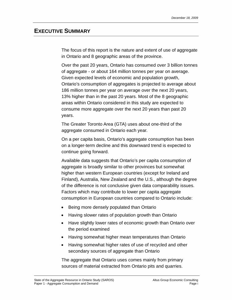
EXECUTIVE SUMMARY

The focus of this report is the nature and extent of use of aggregate in Ontario and 8 geographic areas of the province.

Over the past 20 years, Ontario has consumed over 3 billion tonnes of aggregate - or about 164 million tonnes per year on average. Given expected levels of economic and population growth, Ontario’s consumption of aggregates is projected to average about 186 million tonnes per year on average over the next 20 years, 13% higher than in the past 20 years. Most of the 8 geographic areas within Ontario considered in this study are expected to consume more aggregate over the next 20 years than past 20 years.

The Greater Toronto Area (GTA) uses about one-third of the aggregate consumed in Ontario each year.

On a per capita basis, Ontario’s aggregate consumption has been on a longer-term decline and this downward trend is expected to continue going forward.

Available data suggests that Ontario’s per capita consumption of aggregate is broadly similar to other provinces but somewhat higher than western European countries (except for Ireland and Finland), Australia, New Zealand and the U.S., although the degree of the difference is not conclusive given data comparability issues. Factors which may contribute to lower per capita aggregate consumption in European countries compared to Ontario include:

• Being more densely populated than Ontario

• Having slower rates of population growth than Ontario

• Have slightly lower rates of economic growth than Ontario over the period examined

• Having somewhat higher mean temperatures than Ontario

• Having somewhat higher rates of use of recycled and other secondary sources of aggregate than Ontario

The aggregate that Ontario uses comes mainly from primary sources of material extracted from Ontario pits and quarries.

December 18, 2009

State of the Aggregate Resource in Ontario Study (SAROS) Altus Group Economic Consulting Paper 1 - Aggregate Consumption and Demand Page ii

Imports from other countries play only a small role. Secondary sources of material (primarily recycled materials) have played an increasing role, at about 7% of supply in the past 10 years (up from about 4% in the early 1990s) and recycled material is expected to continue to gradual increase its contribution to total aggregate consumption over the next 20 years. However, assuming no constraints on availability, the main source of aggregate supply is expected to continue to be primary aggregate from Ontario pits and quarries (an average of roughly 171 million tonnes per year compared to 154 million tonnes per year over the past 20 years).

For most of the 8 geographic areas of the province considered in this study, the aggregate consumed mainly comes from primary and secondary aggregate produced locally within those areas. However, that is not the case for the GTA, which obtains approximately half of the aggregate it uses from neighbouring areas.

Both sand and gravel, and crushed stone, are important sources of primary aggregate in Ontario. While crushed stone currently accounts for less than half of the primary aggregate consumed, its role has been increasing and is expected to continue to increase over the next 20 years, given trends in construction standards towards use of higher quality stone.

Aggregate is used for a wide range of applications in Ontario, however the primary use is in construction work - either directly on construction sites, or in the manufacturing of concrete and other building products. Roads (provincial highways, as well as municipal and private roads) account for the largest share of aggregate used in construction work. Some examples of typical amounts of aggregate used in various construction applications include:

• 18,000 tonnes per kilometre of a 2 lane highway in Southern Ontario

• 250 tonnes for a 185 m2 (2,000 sq. ft.) house

• 114,000 tonnes per kilometre of a subway line

Good data exists on local production of primary aggregates in different areas of the province. However, there is currently no comprehensive information available on the internal movements of aggregate between different geographic areas, which makes it

December 18, 2009

State of the Aggregate Resource in Ontario Study (SAROS) Altus Group Economic Consulting Paper 1 - Aggregate Consumption and Demand Page iii

difficult to pinpoint the amounts of aggregate being used in various areas of the province, and in particular the GTA. Estimates of consumption in each geographic area could benefit from a formal survey process undertaken on a periodic basis (similar to one conducted in the UK), to establish movements of aggregate within the province. Such an undertaking would require the buy-in and support of the provincial government, as well as the aggregate industry and possibly key major purchasers of aggregate (such as municipalities) to determine where these consumers obtain their aggregate.

In addition, research by LVM-Jegel suggests that recycled material currently fills roughly 7% of aggregate supply on a province-wide basis, and that the proportion is likely higher in the GTA and major urban areas, and lower in smaller centres. Additional research to better understand the variation in use of recycled material by geographic area in the province would be beneficial.

An initial thought piece on the potential impact of various development patterns and trends was undertaken for this study by MHBC Planning, which showed that there are a wide range of factors that could potentially impact future aggregate consumption per capita – some increasing and some decreasing. Further work in this area to quantify some of these impacts would be beneficial in the projection exercise, in particular to differentiate between short-term and long-term impacts, and between per capita needs for new development versus on-going maintenance and repair.

It is recommended that the projections of aggregate consumption be monitored on a periodic basis (such as every other year) to see how they are tracking, as well as to incorporate where relevant updated projections of economic and population growth.

December 18, 2009

State of the Aggregate Resource in Ontario Study (SAROS) Altus Group Economic Consulting Paper 1 - Aggregate Consumption and Demand Page iv

TABLE OF CONTENTS Page

EXECUTIVE SUMMARY ........................................................................... i

1.0 INTRODUCTION................................................................................ 1 1.1 Report outline .............................................................................................................1 1.2 Geographic areas .......................................................................................................2 1.3 Study limitations..........................................................................................................3 1.4 Definitions ...................................................................................................................3 1.5 A note on aggregate consumption vs. aggregate demand..........................................5

2.0 ONTARIO’S AGGREGATE CONSUMPTION PATTERNS ................ 6 2.1 How much aggregate is used in Ontario? ...................................................................6 2.2 Where does Ontario get the aggregate it uses? .........................................................8 2.3 What are the consumption patterns in different areas of the province? .................... 11

3.0 AGGREGATE CONSUMPTION IN ONTARIO COMPARED TO OTHER AREAS ............................................................................... 16

3.1 A note on comparability of data.................................................................................16 3.2 How does Ontario’s per capita consumption of aggregate compare to other

areas?.......................................................................................................................17 3.3 What factors help explain variations in per capita aggregate consumption?.............20

4.0 THE WAYS IN WHICH AGGREGATE IS USED IN ONTARIO ........ 27 4.1 What are some of the uses of aggregate? ................................................................27 4.2 Which uses are more important in relative terms?....................................................27 4.3 How much aggregate is used per dollar of construction work?.................................32 4.4 How much aggregate does it take for specific construction applications? ................33

5.0 THE FUTURE CONSUMPTION OF AGGREGATE IN ONTARIO ... 35 5.1 How well have past analyses of the future use of aggregate in Ontario

performed? ...............................................................................................................35 5.2 How is future aggregate consumption modelled in other jurisdictions? ....................37 5.3 What is the recommended projection methodology? ................................................38 5.4 What key factors might impact the underlying trend in per capita consumption of

aggregate over the next 20 years? ...........................................................................44 5.5 What is the economic and population growth outlook for the province? ...................58 5.6 What is the projected trend in per capita aggregate consumption? ..........................61 5.7 What is the projected consumption of aggregate in Ontario over the next 20

years? .......................................................................................................................63 5.8 What sources are likely to provide the aggregate used in Ontario over the next

20 years? ..................................................................................................................65 5.9 What alternate scenarios should be considered? .....................................................68

6.0 KEY FINDINGS AND SUGGESTIONS FOR FUTURE WORK ....... 69 6.1 Key findings ..............................................................................................................69 6.2 Suggestions for future work ......................................................................................71

December 18, 2009

State of the Aggregate Resource in Ontario Study (SAROS) Altus Group Economic Consulting Paper 1 - Aggregate Consumption and Demand Page v

Appendix A: Projection Model Background

Appendix B: Aggregate Factors for Specific Construction Applications –Background Calculations

Appendix C: Analysis of Impact of Development Trends on Aggregate Consumption

December 18, 2009

State of the Aggregate Resource in Ontario Study (SAROS) Altus Group Economic Consulting Paper 1 - Aggregate Consumption and Demand Page vi

LIST OF FIGURES Page

Figure 1- 1 SAROS Geographic Areas ...........................................................................2 Figure 2- 1 Average Annual Historical Aggregate Consumption, Ontario........................6 Figure 2- 2 Aggregate Consumption by Year, Ontario.....................................................7 Figure 2- 3 Average Annual Aggregate Consumption Per Capita, Ontario .....................8 Figure 2- 4 Sources of Aggregate Used in Ontario .........................................................9 Figure 2- 5 Annual Primary Production of Aggregate Compared to Total

Consumption, Ontario.................................................................................10 Figure 2- 6 Crushed Stone as a % of Total Consumption of Primary Aggregate,

Ontario........................................................................................................ 11 Figure 2- 7 Total Population and Population Growth by Geographic Area ....................12 Figure 2- 8 Aggregate Consumption by Geographic Area ............................................13 Figure 2- 9 Per Capita Consumption of Aggregate by Geographic Area.......................14 Figure 2- 10 Comparison of Total Aggregate Consumption and Local Primary

Production, Geographic Areas....................................................................14 Figure 3- 1 Per Capita Consumption of Primary Aggregate in Canada by Region........17 Figure 3- 2 Per Capita Primary Aggregate Production, Ontario Compared to U.S.

States .........................................................................................................19 Figure 3- 3 Per Capita Primary Aggregate Consumption, Ontario and Selected

Countries ....................................................................................................20 Figure 3- 4 Comparison of Potential Factors Contributing to Variation in Per Capita

Consumption of Primary Aggregate, Ontario and Selected Countries ........22 Figure 3- 5 Comparison of Potential Factors Contributing to Variation in Per Capita

Production of Primary Aggregate, Ontario and U.S. States ........................25 Figure 3- 6 Comparison of Potential Factors Contributing to Variation in Per Capita

Consumption of Primary Aggregate, Ontario and Other Canadian Regions ......................................................................................................26

Figure 3- 7 Comparison of Potential Factors Contributing to Variation in Per Capita Consumption of Primary Aggregate, Ontario Geographic Areas.................26

Figure 4- 1 Examples of Uses of Aggregate .................................................................28 Figure 4- 2 Use of Aggregate in Construction vs. Other Uses, Ontario.........................28 Figure 4- 3 Aggregate Used in Construction Work, Direct vs. Building Products..........29 Figure 4- 4 Use of Aggregate in Construction Work by Type of Construction, Ontario..30 Figure 4- 5 Uses of Sand and Gravel, Ontario..............................................................31 Figure 4- 6 Uses of Stone .............................................................................................31 Figure 4- 7 Trend in Amount of Aggregate Used Per $1,000 of Construction

Spending, Ontario.......................................................................................32 Figure 4- 8 Amount of Aggregate Used Per $1,000 of Construction Spending by

Type of Construction, Ontario .....................................................................33 Figure 4- 9 Tonnes of Aggregate Used in Specific Construction Applications ...............34 Figure 5- 1 Comparison of Past Ontario Projections of Aggregate Use ........................36 Figure 5- 2 Correlation Analysis, Per Capita Aggregate Consumption and Various

Factors, Ontario, 1980-2008.......................................................................39

December 18, 2009

State of the Aggregate Resource in Ontario Study (SAROS) Altus Group Economic Consulting Paper 1 - Aggregate Consumption and Demand Page vii

Figure 5- 3 Per Capita Aggregate Consumption, Actual vs. Regression Model, Ontario, Average Annual.............................................................................41

Figure 5- 4 Per Capita Aggregate Consumption, Actual vs. Regression Model, Ontario, Annual...........................................................................................41

Figure 5- 5 Province of Ontario Annual Surpluses/Deficits ...........................................46 Figure 5- 6 Assessment of Directional Impact of Selected Emerging Trends on Per

Capita Aggregate Consumption and Use of Higher Quality Aggregate.......53 Figure 5- 7 North Milton Case Study: Key Comparative Indicators ...............................55 Figure 5- 8 Regent Park Case Study: Key Comparative Indicators ..............................57 Figure 5- 9 Projected Average Annual Real GDP Growth, Ontario ...............................58 Figure 5- 10 Projected Average Annual Total Population Growth, Ontario......................59 Figure 5- 11 Projected Average Annual Population Growth Rate, Ontario......................60 Figure 5- 12 Share of Future Population Growth by Geographic Area............................60 Figure 5- 13 Projected Population Growth Rate, Geographic Areas...............................61 Figure 5- 14 Projections of Future Per Capita Aggregate Consumption, Ontario............62 Figure 5- 15 Average Annual Projected Total Aggregate Consumption, Ontario.............63 Figure 5- 16 Projected Total Aggregate Consumption by Geographic Area ....................64 Figure 5- 17 Sources of Aggregate Over the Next 20 Years, Ontario .............................65 Figure 5- 18 Local Primary Production of Aggregate Compared to Total Consumption

of Aggregate, Geographic Areas.................................................................67 Figure 5- 19 Crushed Stone as % of Total Consumption of Primary Aggregate,

Geographic Areas.......................................................................................67 Figure 5- 20 Alternate Scenarios of Future Aggregate Consumption, Ontario ................68

December 18, 2009

State of the Aggregate Resource in Ontario Study (SAROS) Altus Group Economic Consulting Paper 1 - Aggregate Consumption and Demand Page 1

1.0 INTRODUCTION The Ontario Ministry of Natural Resources has undertaken a comprehensive study entitled the State of the Aggregate Resource in Ontario Study, hereafter referred to as simply SAROS. The study request for proposal indicated that:

“The objective of the study [SAROS] is to gain a better understanding of aggregate resources by gathering the most up to date information and current science on the consumption, demand, availability, analysis of alternatives, current reserves, rehabilitation, transportation, recycling/reuse and the value of aggregate to the province of Ontario.”

The broader SAROS work is divided into 6 smaller studies, of which this current report is Paper 1: Aggregate Consumption and Demand.

1.1 REPORT OUTLINE

In addition to this Introduction, the main report contains the following main sections:

• Section 2: Ontario’s Aggregate Consumption Patterns

• Section 3: Aggregate Consumption in Ontario Compared to Other Areas

• Section 4: The Ways in Which Aggregate is Used in Ontario

• Section 5: The Future Consumption of Aggregate in Ontario

• Section 6: Key Findings and Suggestions for Future Work

In addition to the main report, there are a series of separate appendices:

• Appendix A: Projection Model Background

• Appendix B: Aggregate Factors for Specific Construction Applications – Background Calculations

• Appendix C: Analysis of Impact of Development Trends on Aggregate Consumption

December 18, 2009


1.2 GEOGRAPHIC AREAS

The study examines aggregate consumption for the province as a whole, as well as for the province divided into 8 geographic areas. These geographic areas, and their constituent upper or single tier municipalities, are shown on Figure 1- 1.

Figure 1- 1 SAROS Geographic Areas

Area 1 Area 2 Area 3 Area 4

Southwest Peninsula West Central GTA

Essex Niagara Bruce Toronto Chatham-Kent Brant Grey Peel Lambton Haldimand- Simcoe York Elgin Norfolk Dufferin Durham Middlesex Hamilton- Wellington Halton Huron Wentworth Waterloo Perth Oxford

Area 5 Area 6 Area 7 Area 8East Central East Northeast Northwest

Kawartha Lakes Prescott & Russell Nipissing Algoma Peterborough Leeds & Grenville Parry Sound Thunder Bay Haliburton Stormont, Dundas, Timiskaming Kenora Northumberland & Glengarry Cochrane Rainy River Hastings Frontenac Sudbury District Prince Edward Ottawa Sudbury Region Muskoka Lanark Manitoulin

Renfrew Lennox & Addington

December 18, 2009


1.3 STUDY LIMITATIONS

This report relies on information from a variety of secondary sources. While every effort is made to ensure the accuracy of the data, we cannot guarantee the complete accuracy of the information used in this report from these secondary sources.

In addition, due to the lack of comprehensive data for some of the series analyzed, it was necessary as part of this exercise to prepare estimates based on more limited available information.

This report has been prepared solely for the purposes outlined herein and is not to be relied upon or used for any other purposes or by any other party without the prior written authorization of Altus Group Economic Consulting and the Ontario Ministry of Natural Resources.

1.4 DEFINITIONS

This section provides definitions for some terms used throughout the report.

1.4.1 Aggregate related terms

• Aggregate - includes sand, gravel, limestone, dolostone, crushed stone, rock other than metallic ores, and other prescribed material. In this report, aggregate is considered in total, as well as broken into two main groups: 1) sand and gravel 2) crushed stone and other (primarily limestone and dolostone).

• Aggregate consumption – the number of tonnes of aggregate (from both primary and secondary sources, see additional definitions below) used in various applications in a given geographic area during a given time period. As discussed in the report, aggregate consumption in a particular area of Ontario may derive from a variety of sources, including new locally produced aggregate, imports from other provinces and countries, aggregate produced in other areas of Ontario.

• Aggregate demand – see Section 1.5 below. • Per capita aggregate consumption – total consumption

divided by total population.

December 18, 2009


• Primary aggregate production – newly produced aggregate, taken directly from pits and quarries (sometimes also referred to as “virgin” aggregate to differentiate it from recycled and substitute materials). In Ontario, high quality data on primary aggregate production is compiled and reported each year by The Ontario Aggregate Resources Corporation (TOARC).

• Secondary aggregate – recycled aggregate and substitute materials. Data on secondary sources of aggregate are less readily available than for primary aggregate production. In this report, recycling estimates rely on work conducted by LVM Jegel (see Paper 4: Re-use and Recycling).

1.4.2 Acronyms

• GGH - Greater Golden Horseshoe • GDP - gross domestic product (the value of all goods and

services in a given time period; used as a measure of the total size of an economy; “real” GDP expresses output in constant dollar terms that is, adjusts for price inflation)

• GTA – Greater Toronto Area (comprised of the City of Toronto, and the Regional Municipalities of Durham, York, Peel and Halton)

• MNR – Ontario Ministry of Natural Resources

• MNDMF – Ontario Ministry of Northern Development, Mines and Forestry

• OECD – Organisation for Economic Co-operation and Development

• StatCan – Statistics Canada

• TOARC – The Ontario Aggregate Resources Corporation

• UEPG – Union Européenne des Producteurs de Granulats (European Aggregates Association)

• USGS – U.S. Geological Survey

December 18, 2009


1.5 A NOTE ON AGGREGATE CONSUMPTION VS. AGGREGATE DEMAND

The title of the current study, as was outlined in the study Request for Proposal, is “Aggregate Consumption and Demand”.

As outlined in the definitions section, “aggregate consumption” is the term used in reference to the number of tonnes of aggregate actually used in a given area during a given time period.

“Demand for aggregate” is a related, but different, concept. Demand is an economics term which essentially measures how much of a product or service would be purchased/consumed at varying price points (this relationship is the “demand curve”).

As the study progressed, it became clear that the scope of required work as indicated in the Request for Proposal was primarily related to the “consumption” definition – that is, how much aggregate has been used in the past, and might be expected to be used in the future. As such, the term consumption is used almost exclusively in this report.

December 18, 2009


2.0 ONTARIO’S AGGREGATE CONSUMPTION PATTERNS

This section examines past consumption patterns for aggregate in Ontario, in order to answer key questions, including:

• How much aggregate is used in Ontario each year?

• Where does Ontario get the aggregate it uses?

• What are the consumption patterns in different areas of the province?

2.1 HOW MUCH AGGREGATE IS USED IN ONTARIO?

• During the decade of the 2000s (i.e. the 10 year period from 2000 through 2009), Ontario consumed an estimated 179 million tonnes of aggregate on average per year (Figure 2- 1)1.

Figure 2- 1 Average Annual Historical Aggregate Consumption, Ontario

Ontario’s consumption of aggregate has been on a generally upward path since the 1970s

144164

134154 148

179

0

40

80

120

160

200

20 yearsprior tomost

recent

Mostrecent 20

years

1970s 1980s 199 0s 2000s

Estimated average annual consumption, millions of tonnes

Source: Estimates by Altus Group Economic Consulting based o n informa tion from MNDMF, MNR, TOARC, LVM-Jegel,, Stat Can; see Appendix A

1 These consumption estimates are based on data on primary local aggregate production (as measured by TOARC, and previously MNR and MNDMF, production data), as well as estimates of trade in aggregates (imports and exports) from Statistics Canada data and use of recycled material from estimates prepared by LVM-Jegel

December 18, 2009


• This is up from the previous decade (the 1990s) and also higher than either the 1970s or 1980s.

• Over the past 20 years in total, Ontario has consumed over 3 billion tonnes of aggregate.

• Consumption of aggregate can fluctuate significantly from year-to-year (Figure 2- 2). Over the past 40 years, aggregate consumption has ranged from an estimated low of just over 100 million tonnes in recession-ravaged 1982, to over 200 million tonnes in the strong building days of the latter 1980s.

Figure 2- 2 Aggregate Consumption by Year, Ontario

Consumption of aggregate in Ontario can fluctuate year-to-year

131

132 14

11

421

3213

21

32 133

136

123

124

108 11

7 133

153 1

741

94 207

208

170

143

136

139

144

138 1

44 152

153 1

641

8318

017

61

75 183

185 18

91

851

7816

0

0

50

100

150

200

250

71 73 75 77 79 81 83 85 87 89 91 93 95 97 99 01 03 05 07 09e

Estimated annual aggregate consumption, mil lions of tonnes


• The annual level ramped up in the latter 1980s – almost doubling in the space of only 6 years – before dropping back down in the early 1990s.

• After being on a generally upward path since the early 1990s, aggregate consumption has been negatively impacted by the current recession. Similar short-term declines were experienced during the recessions of the early 1980s and early 1990s, before consumption picked up again.

• Over the past 20 years, the total amount of aggregate consumed in the Province of Ontario is equivalent to about 14

December 18, 2009


tonnes per capita on average per year (Figure 2- 3) – about 14% lower than during the previous 20 year period.

Figure 2- 3 Average Annual Aggregate Consumption Per Capita, Ontario

On a per capita basis, Ontario’s consumption of aggregate has been lower in the last 20 years

16.314.0

16.2 16.413.6 14.5

0.0

4.0

8.0

12.0

16.0

20.0

20 yearsprior tomost

recent

Mostre cent 20

years

1970s 1980s 1990s 2000s

Estimated average annual consumption per capita, tonnes


• The per capita pattern, however, has not been consistently downward. During the 1990s, when construction activity had fallen substantially, per capita aggregate consumption fell to below 14 tonnes per year on average, before increasing again during the 2000s.

2.2 WHERE DOES ONTARIO GET THE AGGREGATE IT USES?

• Ontario’s aggregate consumption is filled by two general types of material:

− Primary aggregate: Newly produced sand and gravel, and crushed stone, taken directly from pits and quarries (sometimes referred to as “virgin” aggregate); and

− Secondary aggregate: Recycled aggregate and substitute materials.

December 18, 2009


• Most of the aggregate used in Ontario is primary aggregate (Figure 2- 4). Of the 179 million tonnes of aggregate used each year on average over the past 10 years, it is estimated that about 93% was comprised of primary aggregate.

Figure 2- 4 Sources of Aggregate Used in Ontario

Total aggregate consumption179 million tonnes per year

on average in 2000-2009

Primary materials (93%)

Produced within Ontario (98%)

Imported fromoutside Ontario (2%)

Recycled/secondary materials (7%)

Sand & gravel (59%)

Crushed stone (41%)

Where the aggregate Ontario consumes comes fromWhere the aggregate Ontario consumes comes from

Source: Estimates by Altus Gro up Economic Consult ing based on information from MNDMF, MNR, TOARC, LVM-Jegel,, StatCan; see Appendix A

• While still only a modest contributor to Ontario’s overall aggregate use, the proportion of demand filled by secondary material (essentially recycled material) has grown, up from about 4% in the early 1990s to the current 7%.2

• Primary materials can be either produced locally, or imported from other provinces or countries. However, given the nature of the product, and transportation costs, there is little trade in aggregate between Ontario and other areas.

• Imports to Ontario during the decade of the 2000s accounted for only about 2% of the primary aggregate consumed (or roughly 3

2 The role of recycled material is discussed more fully in SAROS Paper 4: Recycling and Re-use.

December 18, 2009


million tonnes per year).3 The majority of the imports are from the U.S., in particular the states bordering the Great Lakes region (primarily Michigan and Ohio).

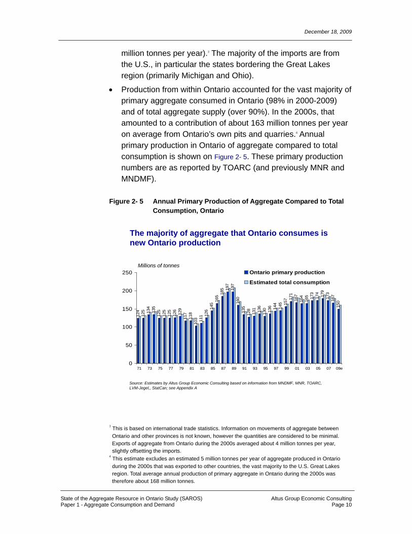
• Production from within Ontario accounted for the vast majority of primary aggregate consumed in Ontario (98% in 2000-2009) and of total aggregate supply (over 90%). In the 2000s, that amounted to a contribution of about 163 million tonnes per year on average from Ontario’s own pits and quarries.4 Annual primary production in Ontario of aggregate compared to total consumption is shown on Figure 2- 5. These primary production numbers are as reported by TOARC (and previously MNR and MNDMF).

Figure 2- 5 Annual Primary Production of Aggregate Compared to Total Consumption, Ontario

The majority of aggregate that Ontario consumes is new Ontario production

124

125 13

413

512

512

512

512

612

911

711

810

3 111 12

6 145

165 18

5 197

197

160

135

128

131 136

130 136 14

414

5 157 17

116

716

416

5 173

174

179

173

167

150

0

50

100

150

200

250

71 73 75 77 79 81 83 85 87 89 91 93 95 97 99 01 03 05 07 09e

Ontario primary production

Estimated total consumption

Millions of tonnes

Source: Estimates by Altus Group Economic Consulting based on information from MNDMF, MNR, TOARC, LVM-Jegel,, StatCan; see Appendix A

3 This is based on international trade statistics. Information on movements of aggregate between Ontario and other provinces is not known, however the quantities are considered to be minimal. Exports of aggregate from Ontario during the 2000s averaged about 4 million tonnes per year, slightly offsetting the imports.

4 This estimate excludes an estimated 5 million tonnes per year of aggregate produced in Ontario during the 2000s that was exported to other countries, the vast majority to the U.S. Great Lakes region. Total average annual production of primary aggregate in Ontario during the 2000s was therefore about 168 million tonnes.

December 18, 2009


• Sand, gravel and crushed stone are all consumed in Ontario. During the decade of the 2000s, slightly more than half of the primary aggregate produced in Ontario was sand and gravel, and slightly less than half was crushed stone.5

• Crushed stone’s relative role in aggregate consumption has been growing over the past 25 years, from a 34% share on average in the latter 1980s to 43% on average per year during the latter 2000s (Figure 2- 6).

Figure 2- 6 Crushed Stone as a % of Total Consumption of Primary Aggregate, Ontario

Crushed stone has been gradually increasing its role in aggregate consumption

30

35

40

45

50

86 87 88 89 90 91 92 93 94 95 96 97 98 99 00 01 02 03 04 05 06 07 08

Source: Estimates by Altus Group Economic Consulting based on information from MNR and TOARC

% of total primary aggregate consumpt ion

2.3 WHAT ARE THE CONSUMPTION PATTERNS IN DIFFERENT AREAS OF THE PROVINCE?

• As discussed in Section 1.2, there are 8 geographic areas within Ontario that were considered for the analysis in this study. To provide context, it is helpful to look at population patterns for those areas.

5 The crushed stone estimates throughout this report include “other” types of aggregate (clay/shale, building stone, industrial stone and dimension stone); these account for only about 2% of all primary aggregate production in Ontario.

December 18, 2009


• The Greater Toronto Area (GTA) – comprised of the City of Toronto, and the Regional Municipalities of Durham, York, Peel and Halton - is the largest of the 8 geographic regions in terms of population, and is currently home to almost half of Ontario’s residents (Figure 2- 7).

• The GTA has also been the growth leader both in absolute and relative terms, accounting for about two-thirds of population growth in the province over the decade of the 2000s.

Figure 2- 7 Total Population and Population Growth by Geographic Area

GTA has captured the majority of population growth in the province in the past 10 years

11 9 11

47

412

3 35 513

68

29

-1 -1-15

0

15

30

45

60

75

90

Southwest

Penin-sula

WestCentral

GTA EastCentral

East North-east

North-west

Share of total population2009Share of populationgrowth past 10 years

%

Source: Altus Group Economic Consulting based on StatC an data; see Appendix A

• Given its sizeable and growing population base, it is not surprising therefore that the GTA accounts for the largest share of total Ontario aggregate consumption (Figure 2- 8) – roughly one-third (or about 61 million tonnes per year) of the 179 million tonnes consumed in Ontario per year in the 2000s.

December 18, 2009


Figure 2- 8 Aggregate Consumption by Geographic Area

Aggregate consumption picked up across the province in the 2000s compared to the 1990s

2115 14

47

7

21

12 11

2218

21

61

8

26

13 12

0

15

30

45

60

75

Southwest

Penin-sula

WestCentral

GTA EastCentral

East North-east

North-west

1990s2000s

Estimated average annual consumption, millions of tonnes

Source: Estimates by Altu s Group Eco nom ic Consu lting; see Appendix A

• All parts of the province saw some increase in consumption of aggregate during the 2000s compared to the 1990s – even those where population growth declined, or was negative. This illustrates the point that while growth is an important driver of the use of aggregate, there is also demand generated from within the existing population base.

• The GTA’s share of aggregate consumption is below its share of population growth and total population, reflecting lower per capita consumption than the Ontario average (Figure 2- 9).

• The highest per capita consumption of aggregate is in Northern Ontario (the Northeast and Northwest geographic areas). As will be discussed later, this in part reflects more intensive use of aggregate in road building due to more severe climate, as well as generally higher use of aggregate per capita in lower density areas due to need for, but less intensive use of, infrastructure.

December 18, 2009


Figure 2- 9 Per Capita Consumption of Aggregate by Geographic Area

GTA consumes less, Northern Ontario more, aggregate per capita

15 15 16

11

16 17

2831

14

0

10

20

30

40

Southwest

Penin-sula

WestCentral

GT A EastCentral

East North-east

North-west

Ontario

Estimated average annual consumption per capita, 2000s, tonnes

Source: Estimates by Altus Group Economic Consulting; see Appendix A

Figure 2- 10 Comparison of Total Aggregate Consumption and Local Primary Production, Geographic Areas

The GTA relies on neighbouring areas for much of the aggregate it uses

1914

36

29

1925

1511

2218

21

61

8

26

13 12

0

15

30

45

60

75

Southwest

Penin-sula

WestCentral

GTA EastCentral

East North-east

North-west

Local primary productionTotal consumption

Estimated average annual, 2000s, millions of tonnes

Source: Estimates by Altus Gro up Economic Consult ing; see Appendix A

December 18, 2009


• For most of the 8 geographic areas, the aggregate consumed comes from primary or secondary aggregate produced locally within those areas (Figure 2- 10).

• However that is not the case for the GTA, which relies on “excess production” from neighbouring areas, in particular the West Central and East Central areas, to provide about half of what it uses.

December 18, 2009


3.0 AGGREGATE CONSUMPTION IN ONTARIO COMPARED TO OTHER AREAS

In this section, Ontario’s relative aggregate usage is compared to other areas of the world. Key questions addressed include:

• How does Ontario’s per capita consumption of aggregate compare to other provinces, U.S. states and other developed countries?

• What factors help explain variation in per capita aggregate consumption?

3.1 A NOTE ON COMPARABILITY OF DATA

• Comparing aggregate consumption across different jurisdictions is a difficult process for a number of reasons, including:

− Information on aggregate consumption is not necessarily collected on a consistent basis, and the coverage and quality of the information can vary substantially from one area to another.

− Information on secondary sources of aggregate are limited and in some jurisdictions even non-existent.

• It was beyond the scope of the analysis here to be able to produce comprehensive information on aggregate consumption in other jurisdictions which is 100% consistent with the relatively high quality of information available for Ontario. Because of data comparability limitations, the comparisons here should be used with caution, and used to identify broad patterns, rather than pinpoint absolute differences.6

• The 2002-2007 period was chosen for the comparisons in this section, as this is the timeframe over which European data was most readily available. Unless otherwise noted, the analysis is

6 To illustrate the difficulties in the comparisons, three sources of information on aggregate production examined for the European data (UEPG’s producers survey, the UK European Mineral Statistics and the USGS Minerals Yearbook), generally showed a wide variation for most countries. The higher of the estimates for each country was used in the analysis here, as it was reasoned that the likelihood of production being underreported was greater than data overstated actual production.

December 18, 2009


limited to consumption of primary sources of aggregate, but including both local production and net imports.

3.2 HOW DOES ONTARIO’S PER CAPITA CONSUMPTION OF AGGREGATE COMPARE TO OTHER AREAS?

This section compares aggregate consumption per capita in Ontario to other areas. An examination of factors which may explain variations in per capita consumption follow in Section 3.3.

3.2.1 Comparison with other Provinces

• Focusing on consumption of primary aggregate only (i.e. excluding recycling and other secondary sources), for the 2002-2007 period, Ontario’s 13 tonnes per capita per year on average is slightly above the Canadian average (Figure 3- 1)7.

Figure 3- 1 Per Capita Consumption of Primary Aggregate in Canada by Region

Ontario’s per capita aggregate consumption is near the Canadian average

10

15

1113 13

9

1412

0

4

8

12

16

20

BC Alta Sask Man Ont Que Atl Canada

Es timated average annual primary* consumption per capita, 2002-2007, tonnes

* Includes local product ion plus net international imports

Source: Estima tes by Altus Group Economic Consulting based on information from StatCan

7 For consistency for the comparison to other provinces, the Ontario data referred to in this section is based on Statistics Canada estimates, which show lower total aggregate production than the TOARC series (which show primary consumption of closer to 14 tonnes per capita for the same period).

December 18, 2009


• Per capita consumption ranged from a low of 9 tonnes per year in Quebec to a high of 15 tonnes per year in Alberta.

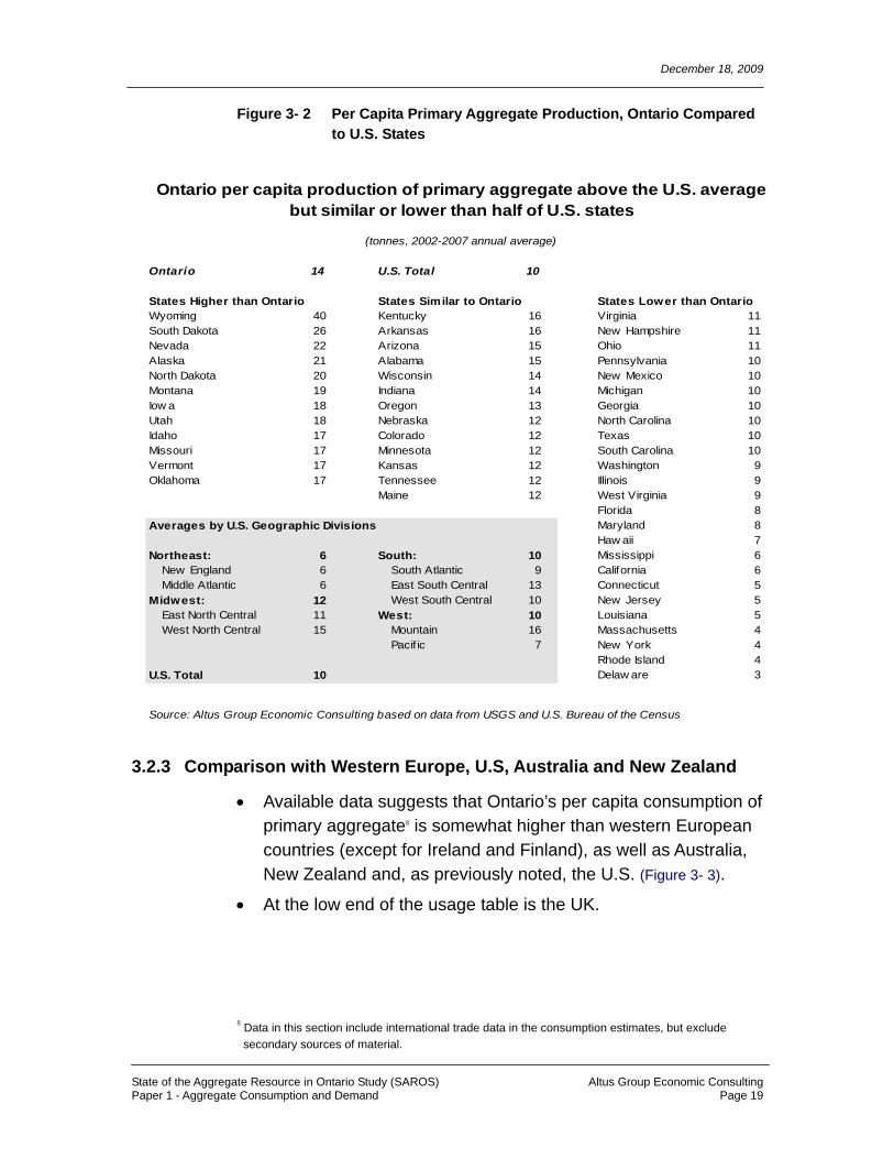
3.2.2 Comparison with U.S. States

• Due to a lack of readily available information on international trade by state, as well as movements of aggregate between states, the comparison of per capita aggregate usage in Ontario with the U.S. is limited to per capita local production. The information for individual states should therefore be viewed with caution, as the generally smaller geographic size of states compared to Ontario could mean a higher potential for some interstate movements.

• The analysis suggests that per capita primary aggregate production in the U.S. over the 2002-2007 period was lower on average than for Ontario.

• The comparison for individual states however shows a wide variation. For about half of the states, per capita aggregate production appears to be below that of Ontario, with the remainder split roughly equally between states with similar per capita production and higher per capita production.

• Factors contributing to the variation by state and comparisons to Ontario are examined in Section 3.3.

December 18, 2009


Figure 3- 2 Per Capita Primary Aggregate Production, Ontario Compared to U.S. States

Ontario 14 U.S. Total 10

States Higher than Ontario States Similar to Ontario States Lower than OntarioWyoming 40 Kentucky 16 Virginia 11 South Dakota 26 Arkansas 16 New Hampshire 11 Nevada 22 Arizona 15 Ohio 11 Alaska 21 Alabama 15 Pennsylvania 10 North Dakota 20 Wisconsin 14 New Mexico 10 Montana 19 Indiana 14 Michigan 10 Iow a 18 Oregon 13 Georgia 10 Utah 18 Nebraska 12 North Carolina 10 Idaho 17 Colorado 12 Texas 10 Missouri 17 Minnesota 12 South Carolina 10 Vermont 17 Kansas 12 Washington 9 Oklahoma 17 Tennessee 12 Illinois 9

Maine 12 West Virginia 9 Florida 8

Averages by U.S. Geographic Divisions Maryland 8 Haw aii 7

Northeast: 6 South: 10 Mississippi 6 New England 6 South Atlantic 9 California 6 Middle Atlantic 6 East South Central 13 Connecticut 5

Midwest: 12 West South Central 10 New Jersey 5 East North Central 11 West: 10 Louisiana 5 West North Central 15 Mountain 16 Massachusetts 4

Pacif ic 7 New York 4 Rhode Island 4

U.S. Total 10 Delaw are 3

Source: Altus Group Economic Consulting based on data from USGS and U.S. Bureau of the Census

Ontario per capita production of primary aggregate above the U.S. average but similar or lower than half of U.S. states

(tonnes, 2002-2007 annual average)

3.2.3 Comparison with Western Europe, U.S, Australia and New Zealand

• Available data suggests that Ontario’s per capita consumption of primary aggregate8 is somewhat higher than western European countries (except for Ireland and Finland), as well as Australia, New Zealand and, as previously noted, the U.S. (Figure 3- 3).

• At the low end of the usage table is the UK.

8 Data in this section include international trade data in the consumption estimates, but exclude secondary sources of material.

December 18, 2009


Figure 3- 3 Per Capita Primary Aggregate Consumption, Ontario and Selected Countries

Ontario per capita aggregate consumption higher than most developed countries

3218

1212

111010

99

988

77

66

64

14

0 5 10 15 20 25 30 35

Irish RepublicFinlandOntarioAustria

DenmarkNew Zealand

SpainUS

PortugalNorwaySweden

NetherlandsAustralia

SwitzerlandFrance

BelgiumItaly

GermanyUK

Per capita, average annual, 2002-2007, tonnes

Source: Altus Group Economic Consulting based on data from UK European Mineral Statistics, UEPG, TOARC, StatCan, USGS and OECD

3.3 WHAT FACTORS HELP EXPLAIN VARIATIONS IN PER CAPITA AGGREGATE CONSUMPTION?

• A variety of factors were examined with respect to the extent to which they play a role in variation in per capita consumption of aggregate.

− Construction spending per capita – as the majority of aggregate is used in construction work, higher rates of construction spending would be expected to generate more aggregate demand per capita. Caution needs to be used in interpreting this variable however, as the mix of work (e.g. engineering vs. building) and relative cost structures (e.g. labour costs vs. materials costs, etc.) are not controlled for.

− Rate of population growth – stronger population growth would be expected to generate more construction work per capita and therefore higher aggregate consumption.

December 18, 2009


− Rate of economic (GDP) growth – to the extent that aggregate is also used in non-construction applications, stronger economic growth may contribute to stronger demand for aggregate on a per capita basis. Real GDP growth also embodies construction spending, as it is a component of GDP.

− Mean annual temperature – geographies with lower average temperatures may need deeper road bases and more repair spending due to more severe weather, which would require higher amounts of aggregate per capita.

− Population density – more densely populated areas may use less aggregate on a per capita basis.

− Extent of use of secondary aggregate – as there is no comprehensive data on secondary aggregate consumption for all of the areas covered, this is considered as an explanatory factor (rather than being included in consumption) – greater use of secondary material reduces the use of primary material.

• Information for these factors where available are summarized on the following chart (Figure 3- 4) for the international comparison. Similar charts follow at the end of this section comparing Ontario to U.S. states (Figure 3- 5), other provinces (Figure 3- 6), as well as comparing the Ontario geographic areas (Figure 3- 7).

• Using this information, a correlation analysis was conducted which shows the direction and strength of the relationship between each factor and primary aggregate consumption per capita. Correlation analysis shows whether patterns tend to move in the same or opposite directions and the strength of the relationships of the movements.

• The analysis (see bottom line of Figure 3- 4) confirmed the relationships outlined above in terms of their directional impact (for example, a negative sign for mean temperature indicates that lower mean temperature is associated with higher aggregate consumption per capita although the degree of the relationship is not particularly strong). It should be emphasized

December 18, 2009


that correlation is not the same as causation; rather it shows if two factors move together but not whether one factor is causing the other to occur.

Figure 3- 4 Comparison of Potential Factors Contributing to Variation in Per Capita Consumption of Primary Aggregate, Ontario and Selected Countries

Per capita primary

aggregate consumption

Population growth

rate

Real GDP growth

rate

Real GDP per

capita

Real construc-

tion spendng

per capita

Mean temp Density

Secondary aggregates

tonnes % % $000s $000s degrees pop/sq. km %2002-07 2002-07 2002-07 2002-07 2002-07 Celsius 2005/06 2005/06

Ontario 14 1.2 2.4 32 3.1 9 13 7

Selected countries

Irish Republic 32 2.0 5.6 34 5.4 10 59 1Finland 18 0.3 3.2 29 3.2 5 16 1Austria 12 0.5 2.4 30 3.5 11 98 6Denmark 12 0.3 1.8 30 3.0 8 126 naNew Zealand 11 1.4 3.5 23 2.6 14 15 naSpain 10 1.6 3.4 23 3.5 15 86 0US 10 0.9 2.6 37 3.3 15 32 naPortugal 9 0.5 0.9 17 2.1 17 114 naNorw ay 9 0.7 2.4 39 2.7 6 14 0Sw eden 9 0.5 3.1 31 1.9 7 20 6Netherlands 8 0.3 1.9 31 3.3 10 400 21Australia 8 1.4 3.3 30 4.1 13 3 naSw itzerland 7 0.7 2.1 33 2.5 10 180 9France 7 0.7 1.8 27 3.1 12 111 5Belgium 6 0.5 2.2 29 2.8 10 342 19Italy 6 0.4 1.0 26 2.7 16 193 2Germany 6 0.0 1.2 27 2.6 10 231 14UK 4 0.5 2.6 29 2.5 11 245 25

0.6 0.7 0.2 0.7 -0.3 -0.4 -0.5

Source: Altus Group Economic Consulting based on data from UK European Mineral Statistics, UEPG, TOARC, StatCan, USGS and OECD

Correlation with primary aggregate consumption

Selected characteristics

December 18, 2009


• Some broad conclusions can be drawn from the analysis.

• Those countries towards the bottom of the usage chart (under 9 tonnes per capita) tend to have characteristics that help explain lower per capita primary aggregate consumption than Ontario, including:

− Being more densely populated than Ontario (except for Australia), even if the Northern area of Ontario is excluded;9

− Having slower rates of population growth (except for Australia)

− Have slightly lower rates of GDP growth over the period (except UK and Australia), and slightly lower GDP per capita (except for Switzerland)

− Having somewhat higher mean temperatures

− Having higher rates of use of secondary aggregate (except for France and Italy).

• However a key factor that does not appear to be consistent is the comparison of the per capita construction spending estimates. In general, per capita construction spending is only slightly lower in the countries with substantially lower aggregate consumption per capita than Ontario. This is puzzling if construction spending is a key driver of aggregate usage. It may be due to differences in the mix (i.e. a relatively higher share of the Ontario construction spending in more aggregate intensive uses), as well as the fact that these numbers include only new work (i.e. repair work is not included). But it might also suggest that there is understatement in the European numbers/coverage relative to the Ontario production data series.

• Ireland stands out as having much higher aggregate consumption per capita than any other country. This in large part however likely reflects the timeframe for the analysis. The period of 2002-2007 was a period of exceptionally strong population and economic growth and strong construction spending (refer to

9 Excluding the Northeast and Northwest areas increases Ontario density to about 108 persons per sq. km.

December 18, 2009


Figure 3- 4). With weaker economic conditions post 2007, it is likely that Ireland’s per capita aggregate consumption has moderated from this level.

• What has not been built into the quantitative analysis here however is potential policy impacts. For example, the U.K. has the lowest per capita primary aggregate consumption, but also unlike other countries examined, has a very sizeable aggregate levy (currently 2 pounds sterling per tonne, or roughly $3.50 Canadian10 – this compares to the $0.11 per tonne licence fee in Ontario). To what extent this may have altered aggregate consumption patterns – and/or encouraged underreporting of primary production – is unclear. It is even unclear whether the relatively high use of secondary material is a function of the levy, as trends to higher recycling appear to have been occurring prior to the introduction of the levy.

10 Based on an exchange rate of $1.73 Canadian dollars per UK pounds sterling (as of December 18, 2009)

December 18, 2009


Figure 3- 5 Comparison of Potential Factors Contributing to Variation in Per Capita Production of Primary Aggregate, Ontario and U.S. States

Per capita primary

aggregate production

Population growth

rate

Real GDP growth

rateMean temp Density

tonnes % % degrees pop/sq. km2002-07 2002-07 2002-07 Celsius 2005/06

Ontario 14 1.2 2.4 9 13

StateWyoming 40 1.0 2.6 7 2 South Dakota 26 0.8 3.3 8 4 Nevada 22 3.4 5.4 20 7 Alaska 21 1.2 2.9 5 0 North Dakota 20 0.0 3.6 5 4 Montana 19 0.9 3.7 7 2 Iow a 18 0.3 3.1 10 20 Utah 18 2.6 4.1 11 10 Idaho 17 2.1 4.1 11 6 Missouri 17 0.7 1.3 12 31 Vermont 17 0.2 2.3 7 25 Oklahoma 17 0.7 2.5 16 19 Kentucky 16 0.7 2.3 13 39 Arkansas 16 0.9 2.7 16 20 Arizona 15 3.1 4.5 23 17 Alabama 15 0.6 2.9 18 34 Wisconsin 14 0.6 1.6 7 38 Indiana 14 0.6 1.5 11 65 Oregon 13 1.2 4.5 11 14 Nebraska 12 0.5 2.8 10 9 Colorado 12 1.5 2.1 10 16 Minnesota 12 0.7 2.4 7 24 Kansas 12 0.5 2.4 12 13 Tennessee 12 1.1 2.8 15 53 Maine 12 0.4 1.6 7 16 Virginia 11 1.2 2.9 14 69 New Hampshire 11 0.7 2.0 7 53 Ohio 11 0.1 1.1 11 107 Pennsylvania 10 0.2 1.7 12 106 New Mexico 10 1.2 3.0 13 6 Michigan 10 0.1 0.2 9 68 Georgia 10 2.1 2.3 16 55 North Carolina 10 1.6 3.2 15 64 Texas 10 1.9 3.3 20 31 South Carolina 10 1.4 1.9 17 51 Washington 9 1.2 2.9 11 34 Illinois 9 0.4 1.5 11 86 West Virginia 9 0.1 1.3 13 29 Florida 8 1.8 3.9 20 114 Maryland 8 0.7 2.9 13 209 Haw aii 7 0.8 3.5 25 73 Mississippi 6 0.4 1.9 18 23 California 6 0.9 3.2 16 84 Connecticut 5 0.3 2.0 11 271 New Jersey 5 0.3 1.6 13 438 Louisiana 5 -0.3 2.6 20 40 Massachusetts 4 0.2 1.7 11 313 New York 4 0.3 3.0 9 155 Rhode Island 4 -0.1 2.1 10 387 Delaw are 3 1.4 2.2 13 155

0.3 0.3 -0.3 -0.6

Selected Characteristics

Correlation with primary aggregate production

Source: Altus Group Economic Consulting based on data from USGS and U.S. Bureau of the Census

December 18, 2009


Figure 3- 6 Comparison of Potential Factors Contributing to Variation in Per Capita Consumption of Primary Aggregate, Ontario and Other Canadian Regions

Per capita prim ary

aggregate cons um ption

Population grow th

rate

Real GDP grow th

rateM ean tem p Dens ity

tonnes % % degrees pop/sq. km2002-07 2002-07 2002-07 celsius 2005/06

Ontario 14 1.2 2.4 9 13

Other regionsAtlantic 14 0.6 2.9 5 5Quebec 9 0.6 2.1 4 6Manitoba 13 1.6 2.4 3 2Saskatchewan 11 1.8 2.5 3 2Alberta 15 0.8 3.9 2 5B.C. 10 0.7 3.6 10 4

Note: mean temperatures are b ased on provincial capitals


Source: Altus Group Economic Consulting based on data from TOARC and StatCan

Figure 3- 7 Comparison of Potential Factors Contributing to Variation in Per Capita Consumption of Primary Aggregate, Ontario Geographic Areas

Per capita prim ary

aggregate consum ption

Population grow th

rate Dens itytonnes % pop/sq. km

2002-07 2002-07 2005/06

Ontario 14 1.2 13

By Geographic SubareaArea 1: Southwest 14 0.6 68Area 2: Peninsula 14 0.6 167Area 3: W est Central 15 1.6 69Area 4: GTA 10 1.8 780Area 5: East Central 15 0.8 22Area 6: East 17 0.7 51Area 7: Northeast 27 -0.1 2Area 8: Northwest 31 -0.3 1

Ontario excluding North 13 1.3 108


Source: Altus Group Economic Consulting based on data from TOARC and StatCan

December 18, 2009


4.0 THE WAYS IN WHICH AGGREGATE IS USED IN ONTARIO The preceding section examined the extent to which Ontario uses aggregate each year. This section examines the ways in which aggregate is being used. Key questions to be answered in this section include:

• What are some of the uses of aggregate?

• Which uses are more important in relative terms?

• How much aggregate is used per dollar of construction work?

• How much aggregate does it take for specific construction applications?

4.1 WHAT ARE SOME OF THE USES OF AGGREGATE?

• Aggregate can be used in a variety of applications, including various types of construction work and manufactured products.

• Some of the uses of aggregate are outlined in Figure 4- 1.

4.2 WHICH USES ARE MORE IMPORTANT IN RELATIVE TERMS?

• Unfortunately, data is not available to quantify the amounts of aggregate that go into each of the specific uses identified on Figure 4- 1. However, we can look at their relative roles on a higher, more aggregated level using information from Statistics Canada’s Input-Output model of the Canadian economy.

• Construction work accounts for the majority of aggregate consumed in Ontario. During the 2000s, an estimated 81% of the total aggregate consumed in Ontario was used in various construction applications (Figure 4- 2).

• Some of this was aggregate that went directly into construction work (about two-thirds of total construction related aggregate); the remainder was indirectly used in construction, through building products such as ready-mix concrete, manufactured concrete products, and other building materials such as roofing tiles (Figure 4- 3).

December 18, 2009


Figure 4- 1 Examples of Uses of Aggregate

Aggregate is used in many different applications

container packaging

cosmetics

crushed glass (for water filtration)

concrete aggregate

catalytic converters

carpet

buildings (office, hospital, schools)

bridges

bake & culinary ware

backfill for mines

automotive & vehicular glass & glazing

automobiles and aircraft parts

automotive frames

asphalt aggregate

agricultural soil supplements

agricultural purposes and fertilizer plants

abrasive cleanser emergency flood retention fibre glass

flat glass

flux in iron and steel plants

housing

ice control (road sand)

industr ial flue scrubbers

landfill cover

landscaping

light bulbs

lime kilns

medical research instruments

metal cast moulding

metal casting

mild abrasive

military field fortification

mirrors

monumental and ornamental

mortar sandparking lotspharmaceuticals

photovoltaics

piers & wharfs

pipes (main and sewers)

power plants

pulp and paper mills

railway ballast

railway bedding

recreational sand

glass tile

retention walls

riverbed lining

road metal

roads & highways

roads: Ice control

roads: road bed, surface

roofing granules

shoreline protection

sidewalks

soil remediation

streetcar & tram brake systems

stucco dash

subway tunnels

sugar refineries

surgery instruments

tableware

toothpaste

tunnels

TV & computer screens

washing detergent

water filtration

wind turbines

septic system/beds

rubble and riprap

runways

Sandblasting

Source: Compiled by Altus Group Economic C onsulting based on synthesis of many documents (see Reference list)

Figure 4- 2 Use of Aggregate in Construction vs. Other Uses, Ontario

Construction work is the major use for aggregate

81%

19%

Construction work

Other uses

Source: Estimates by Altus Group Economic Consulting based on StatCan 2005 N ational Input-Output model

% of total aggregate use, Ontario, 2000-2009

December 18, 2009


Figure 4- 3 Aggregate Used in Construction Work, Direct vs. Building Products

Aggregate is used both directly in construction, and in the manufacturing of building products

Ready mix concrete, 21%

Concrete products, 7%

Other building products, 10%

Directly used in construction,

62%

% of total construction-related aggregate, Ontario, 2000-2009

Source: Estimates by Altus Group Economic Consulting based on StatCan 2005 National Input-Output model

• The use of aggregate in construction work can be further disaggregated by type of construction work.

• During the 2000s, new road construction in Ontario accounted for an estimated one-third of construction-related aggregate use (Figure 4- 4). Construction repair work accounted for another 14%. As roads are estimated to account for most of the aggregate use related to repair work, this suggests that, combined, new and repair/maintenance road work account for close to half of aggregate used in construction work.

• It is important to note that the public sector plays a key role in aggregate consumption through its roadbuilding and other infrastructure related programs (most of which is included in “new other engineering”).

December 18, 2009


Figure 4- 4 Use of Aggregate in Construction Work by Type of Construction, Ontario

Roads consume the largest share of aggregate used in construction work

26

15

34

1014

0

10

20

30

40

New residential New non-residential

building

New roads* New otherengineering

Repairconstruction**

Estimated share of construction-related aggregate by type of construction2000-2009

* Includes municipal, provincial and private sector road spending**While a breakdown is not available in the input-output model, the majority of aggregate used in repair work is estimated to be for road repairs


• The information available from the analysis of the National Input-Output model can be supplemented with StatCan survey information to gain some additional insight into the relative importance of specific uses of aggregate.

• Information is collected from producers on known uses of aggregate (Figure 4- 5 and Figure 4- 6).

• While not as comprehensive as one might like (in particular, there are substantial portions of “unspecified” uses, in part as the producers often would not have the information on the end use by the purchasers), it does confirm that road construction and concrete are key uses of aggregate.

December 18, 2009


Figure 4- 5 Uses of Sand and Gravel, Ontario

Road construction a primary use of sand and gravel

30.011.4

6.63.9

2.01.8

1.10.6

42.7

0 10 20 30 40 50

Roads: Road bed, surface

Concrete aggregate

Fill

Asphalt aggregate

Mortar sand

Roads: Ice control

Backfill for mines

Railroad ballast

Unspecified uses

% of total uses of sand & gravel, 2006, Ontario

Source: Altus Group Economic Consulting based on StatCan, Non-Metallic Mineral Mining and Quarrying (Catalogue 26-226)

Figure 4- 6 Uses of Stone

Road metal and concrete key uses of stone

21.912.4

8.42.3

1.61.31.1

0.6

0.00.00.0

25.9

23.6

0.1

0.40.1

0.4

0 5 10 15 20 25 30

Road metal

Concrete aggregate

Cement

Asphalt aggregate

Lime kilns

Pulverized stone for agricultural and other

Other chemical process

Railway ballast

Dimensional stone

Roofing granules

Rubble and riprap

Flux in iron and steel plants

Pulp and paper mills

Sugar refineriesGlass factories

Stucco dash

Unspecified uses

% of total uses of stone, 2006, Canada*

* Note: data on this chart are for Canada, as comparable information is not published specifically for Ontario

Source: Altus Group Economic Consulting based on StatCan, Non-Metallic Mineral Mining and Quarrying (Catalogue 26-226)

December 18, 2009


4.3 HOW MUCH AGGREGATE IS USED PER DOLLAR OF CONSTRUCTION WORK?

• For every $1,000 spent on construction work during the 2000s, there was a corresponding use of about 3.2 tonnes of aggregate (primary and secondary combined) on average per year (Figure 4- 7). 11

Figure 4- 7 Trend in Amount of Aggregate Used Per $1,000 of Construction Spending, Ontario

The amount of aggregate per $1,000 of construction work has been declining

2.5

3.0

3.5

4.0

4.5

81 82 83 84 85 86 87 88 89 90 91 92 93 94 95 96 97 98 99 00 01 02 03 04 05 06 07 08

Tonnes per $1,000 of total construction spending ($2002)

Source: Estimates by Altus Group Economic Consulting based on information from MNR,TOARC and StatCan

1980s - 3.71990s - 3.42000s - 3.2

• The tonnes of aggregate used per $1,000 of total construction spending however has been on a generally downward trend since the early 1980s.12

• The amount of aggregate used per $1,000 of spending varies by type of construction work, with significantly more aggregate being used per dollar spent on road construction than other types of construction work (Figure 4- 8).

11 Note that no adjustment has been made here to exclude aggregate used in non-construction activity, due to lack of comprehensive information on annual trends in that component.

12 The pronounced lower intensity levels in the early 1990s reflected that construction spending during that period was primarily work that lingered from the non-residential overbuilding in the latter 1980s; much of the initial stages of work on these buildings (aggregate is typically used in the earlier stages of this type of work) would have been completed by the early 1990s.

December 18, 2009


Figure 4- 8 Amount of Aggregate Used Per $1,000 of Construction Spending by Type of Construction, Ontario

More aggregate used per dollar of spending on roads than other types of construction

1.3 1.9

20.5

2.2 2.7

0

5

10

15

20

25

New residential New non-residential

building

New roads New otherengineering

Repairconstruction*

* While a breakdown is not available in the input-output model, the majority of aggregate used in repair work is estimatedto be for road repairs

Estimated tonnes per $1,000 of construction spending ($2002)


4.4 HOW MUCH AGGREGATE DOES IT TAKE FOR SPECIFIC CONSTRUCTION APPLICATIONS?

• As part of the work for this project, estimates of the amounts of aggregate required for specific applications were prepared.13

• Unlike the dollar spending basis approach used in the previous section, the analysis in this section focuses on aggregate needed for a particular physical “quantity” of construction work.

• The results are summarized on Figure 4- 9. Highlights include:

− 18,000 tonnes of aggregate per kilometre of a 2 lane highway in Southern Ontario

− 250 tonnes for a 185 m2 (2,000 sq. ft.) house

− 114,000 tonnes per kilometre of a subway line

13 This analysis was conducted primarily by LVM-Jegel, based on construction projects undertaken by the firm and its affiliated companies. The specific assumptions underlying the construction of the factors are provided in Appendix B.

December 18, 2009


Figure 4- 9 Tonnes of Aggregate Used in Specific Construction Applications

Roads (per km) Tonnes

2 lane highway 18,0004 lane highway 30,0004 lane freeway 44,000

Major arterial road:Southern Ontario 18,000Northern Ontario - typical 13,500Northern Ontario - high volume 24,000

Minor arterial road:Southern Ontario 7,500Northern Ontario - typical 13,500Northern Ontario - high volume 22,000

Collector:Southern Ontario 14,000Northern Ontario - typical 12,500Northern Ontario - high volume 22,000

Local:Southern Ontario 6,500Northern Ontario - typical 12,000Northern Ontario - high volume 21,000

Laneway 6,500

Buildings and parking Tonnes

House (185 m2) 250

Office, school, hospital space (1,000 m2) 730

Parking (per space)Underground parking garage 9Above ground suspended slab 7At grade 15

Underground water pipe and sewer line (per km) Tonnes

Underground water pipe - under a boulevardSouthern Ontario 1,000Northern Ontario 1,000

Underground water pipe - under a roadSouthern Ontario 3,000Northern Ontario 4,500

Underground sewer line - under a boulevard 2,500Underground sewer line - under a road 14,500

Miscellaneous infrastructure Tonnes

4 lane concrete bridge over 6 lane highway (83 meters) 7,500

Railway bed (per km) 6,000

Rural septic/filter bed 85

Wind turbine 4,000

Subway line (per km) 114,000

Nuclear power plant 136,000

Source: LVM-Jegel (see Appendix B) and AECOM Canada (see subway case study in SAROS Paper 3 - The Value of Aggregates)

December 18, 2009


5.0 THE FUTURE CONSUMPTION OF AGGREGATE IN ONTARIO This section examines the prospects for future consumption of aggregate in Ontario as a whole, and for each of the 8 geographic areas. Key questions addressed include:

• How well have past analyses of the future use of aggregate in Ontario performed?

• How is future aggregate consumption modelled in other jurisdictions?

• What is the recommended projection methodology?

• What key factors might impact the underlying trend in per capita consumption of aggregate over the next 20 years?

• What is the economic and population growth outlook for the province?

• What is the projected trend in per capita aggregate consumption?

• What is the projected consumption of aggregate in Ontario over the next 20 years?

• What sources are likely to provide the aggregate used in Ontario over the next 20 years?

• What alternate scenarios should be considered?

5.1 HOW WELL HAVE PAST ANALYSES OF THE FUTURE USE OF AGGREGATE IN ONTARIO PERFORMED?

• Projections of the future consumption of aggregate are not a new situation in the Province of Ontario. Several past exercises have been undertaken for the Ministry of Natural Resources that have tried to “predict” what the future holds.14

• For the most part, these projections have tended to overstate future use (Figure 5- 1). Some factors behind the poor track record include:

− In some cases the models themselves were not the best choice. The most recent of these past projections for

14 A summary of these past studies is provided in Appendix A.

December 18, 2009


MNR was almost 20 years ago. The historical series available at that time to help in the modelling exercise was more limited – that is, shorter term information by necessity had to be used to project longer-term trends.

− Like the situation for projections in general, the world does not always unfold as expected – that is, while the model may have been reasonable, the inputs/assumptions used to derive the outputs were not what actually occurred. For example, when the last exercise was conducted for MNR in 1992 (the State of the Resource Study, or SOTR), the general view was that Ontario would quickly recover from the recession of the early 1990s; this did not however occur, and construction levels remained constrained through the rest of the decade.

Figure 5- 1 Comparison of Past Ontario Projections of Aggregate Use

Past projections have in general overstated future aggregate use in Ontario

200

154125

199

166142 145 146 156 164

0

50

100

150

200

250

1974 Proctor &Redfern (1974-2001)

1980 Peat Marwick(1980-2000)

1982 Matten (1981-2000)

1992 Clayton SOTR(1991-2010)

1996 Clayton Update(1996-2010)

Projected Actual

Average annual total use of primary aggregate, tonnes (millions), Ontario

Note: the years in parentheses indicate the timeline for the projections

Source: See List of References

• Given the poor track record in general on projecting future aggregate consumption for the province, one might well ask “Why do it?”. The answer is that a view of the future is necessary in order to plan for what might unfold. The key in

December 18, 2009


projections, however, is to keep them dynamic – easily and readily updateable if and when the real world starts to veer from the projected world.

• Moreover, as already indicated, there is more information available today to help in the projection exercises than was the case when previous projections were prepared. The additional years of historical information provide a sounder basis on which to assess past trends, and how they might apply to the future.

5.2 HOW IS FUTURE AGGREGATE CONSUMPTION MODELLED IN OTHER JURISDICTIONS?

• Ontario has been among the frontrunners in the world in terms of commissioning work to model the future consumption of aggregate.

• Many other jurisdictions do not even attempt to do so. Among those that do, methods generally fall under 3 main categories:15

− Historical trend: using such simple assumptions as recent per capita consumption or recent average annual levels (the California model uses this approach)

− Regression models: using either macroeconomic indicators (such as GDP, population, unemployment rate, etc.) or based on construction spending (this was the previous UK methodology; it was also used in the 1992 State of the Resource Study as a short-term projection method as this method tends to identify turning points better than other methods)

− Construction input factors: these may be either space-based (i.e. tonnes per sq. ft. of different types of construction; previous work for the Lower Mainland in B.C. took this approach) or dollar-based factors (i.e. tonnes per dollar spending), for different types of construction (the approach used in the 1992 State of the Resource Study).

15 A concise summary of various models used in past Ontario studies as well as more recent ones for other jurisdictions, is provided in Appendix A.

December 18, 2009


5.3 WHAT IS THE RECOMMENDED PROJECTION METHODOLOGY?

5.3.1 The Per Capita Approach

• The following key principles were considered in terms of choosing the appropriate modelling methodology for this exercise:

− The model should not be overly complicated - the methodology should be relatively easy to understand, and not a “black box”.

− Any data required to operationalize and update the model should be readily available, with external updates of key inputs available preferably on an annual basis, or at least every few years.

− The methodology should lend itself to sensitivity testing and formulation of alternate scenarios.

• With these principles in mind, it was recognized that a methodology that was built on assumptions about per capita use of aggregate might best fit these criteria:

− Applying a per capita aggregate consumption assumption to total population is a relatively simple process.

− The key data require for the exercise is readily available, as long-term projections of total population are prepared on a regular basis by the Ontario Ministry of Finance, for Ontario as a whole as well as for each census division, which can then be compiled into projections for each of the 8 geographic areas.16

− Sensitivity testing can be easily done on alternate population scenarios as the Province’s projections include base case, low and high scenarios. Alternate assumptions about the per capita level can also be easily applied.

16 While previously these projections were prepared only every few years, in the latest population projections document (Ontario Population Projections, 2008-2036) it is stated that “The new projections will be updated every year in future to provide planners and researchers with a demographic outlook reflecting the most up-to-date trends and historical data” (pg. 3)

December 18, 2009


• It was also recognized however that a constant per capita assumption would not be reasonable. As shown previously, over the longer-term, per capita usage has been gradually declining. However, it also tends to be above trend in periods of stronger economic activity, and below trend in periods of weaker economic activity.

• It was felt that regression analysis could prove useful in helping to determine the future trends in per capita aggregate consumption. Regression analysis statistically identifies the relationship between an independent variable (in this case, per capita consumption of aggregates in Ontario) and a set of independent variables. The potential independent variables considered for the analysis here included total population, population growth, housing starts, real GDP growth (%) and the unemployment rate. These variables were the focus, as they are all variables contained in typical long-term Ministry of Finance economic projections.

• To begin, a correlation analysis was done for these variables for the 1980-2008 period (Figure 5- 2).

Figure 5- 2 Correlation Analysis, Per Capita Aggregate Consumption and Various Factors, Ontario, 1980-2008

Total population

(000s)

Total population

growth (000s)

Unemployment rate

%

Housing starts (000s)

Real GDP growth

(%)

Per capita total

aggregate consumption

(tonnes)Total population (000s) 1.00

Total population growth (000s) 0.22 1.00

Unemployment rate % -0.28 -0.51 1.00

Housing starts (000s) 0.30 0.70 -0.71 1.00

Real GDP growth (%) -0.13 0.03 -0.25 0.16 1.00

Per capita total aggregate consumption (tonnes) -0.19 0.69 -0.68 0.79 0.26 1.00

Source: Altus Group Economic Consulting based on data from MNR, TOARC and StatCan

December 18, 2009


• The analysis confirmed that these factors are all correlated with per capita aggregate consumption to some degree and have the expected positive or negative signs:

− Total population has a moderate, negative correlation, meaning that as total population increases, the per capita amount of aggregate used declines.

− Population growth (number of persons) has a higher correlation with per capital aggregate consumption than total population, and the sign is positive, as expected.

− The unemployment rate is highly correlated with per capita aggregate consumption, and the sign is negative (i.e. an increase in the unemployment rate would be expected, all other things being equal to be associated with a decline in per capita aggregate consumption).

− Housing starts are highly correlated with per capita aggregate consumption, and the sign is positive – the higher the level of housing starts, the higher the level of per capita aggregate consumption.

− The rate of real GDP growth is moderately correlated with per capita aggregate consumption, and the sign is positive (i.e. stronger economic growth is associated with higher per capital consumption).

• Based on this correlation analysis, all of the independent variables identified above were included in the regression analysis conducted for the 1980-2008 period.17

• The overall fit of the model was very good, with an adjusted R2 of 89%. All of the independent variables were shown to be statistically significant, with the exception of real GDP growth (the latter variable however was kept in the model as removing it reduced the overall model fit).

• The resulting model was used to “project” historical consumption, to see how well it did for the longer term (10 year), medium term (5 year) and short-term (annual).

17 The key model statistics, as well as the annual data used to conduct the regression analysis, are provided in Appendix A.

December 18, 2009


Figure 5- 3 Per Capita Aggregate Consumption, Actual vs. Regression Model, Ontario, Average Annual

The model performed well on 10 year historical periods, less well on recent 5 year periods

16.4

13.614.5

13.5

19.3

13.9 13.414.9 14.5

16.4

13.414.5 14.1

18.7

13.5 13.3

15.6

13.4

0

5

10

15

20

25

1980s 1990s 2000s 1980-1984

1985-1989

1990-1994

1995-1999

2000-2004

2005-2009

Actual Fitted by the model


Source: Altus Group Economic Consulting based on information from MNR, TOARC and StatCan

Figure 5- 4 Per Capita Aggregate Consumption, Actual vs. Regression Model, Ontario, Annual

The model generally able to “predict” broad turning points

11

13

15

17

19

21

1979 1983 1987 1991 1995 1999 2003 2007

Actual per capitaconsumptionValues fitted by themodel

Source: Altus Group Economic Consulting based on information from MNR, TOARC and StatCan

Annual aggregate consumption per capita, tonnes

December 18, 2009


• The fit for the longer-term 10 year basis was quite good, with results closely matching the actual per capita consumption (Figure 5- 3). The medium-term 5 year basis was also fairly close, although the model tended to “overpredict” per capita aggregate consumption in the early 2000s, and “underpredict” the latter 2000s. This pattern for early vs. latter 2000s was also exhibited in the annual results (Figure 5- 4). It is likely that spending under the government stimulus program, which is not directly captured in the model, is playing a role in the short-term.

• Given the above, it was decided that the per capita approach would be adopted for this study. The regression model was used to do initial runs of per capita usage, however consideration was also given to potential factors outside the model variables that might impact future trends in per capital aggregate usage. An analysis of those factors is conducted in Section 5.4.

5.3.2 Why a construction spending approach not adopted for use in this study

• Since construction spending is the primary user of aggregate, serious consideration was given to using a projection approach which first projects construction spending by type of construction, and then applies factors showing the amount of aggregate used per dollar of various types of construction spending. This was the approach used in the 1992 State of the Resource Study.

• This methodology, however, does not meet one of the key criteria, which is that the data needed to operationalize the model should be readily available. Indeed, it falls short in several areas in this respect:

− The methodology requires generating factors on the amount of aggregate used per dollar spending of various types of construction activity. These factors are generally obtained from Statistics Canada’s Input-Output model. However, the level of detail required by type of construction work, and for the actual aggregate products (sand & gravel and crushed stone) are only available at the national level, not specific to Ontario. Therefore

December 18, 2009


several assumptions and adjustments are required to operationalize the model for Ontario.

− The model requires a good series on historical Ontario construction spending by type of construction, and for new and repair/maintenance work, in order to determine what the historical usage factors are (i.e. the amount of aggregate per dollar of various types of construction spending). While the provincial economic accounts provide information on new construction spending, total non-residential construction is not broken down into building, road engineering and other engineering (which is needed, since as shown in Section 4.3, the amount of aggregate per dollar of spending varies by type of construction). Similarly, projections of construction spending at the level required for the methodology are not readily available, and would need to be independently generated as part of the projection exercise.

− As the amount of aggregate used per dollar of construction spending has been declining over time (as shown in Section 4.3), adjustments would need to be made to the factors over time.

− Adjustments/assumptions need to be made for non-construction uses as well, based on limited historical information.

• Also, while construction spending is a good predictor of aggregate usage over longer period, it performs less well in identifying short-term turning points. That is because construction spending series are based on “work put in place” through the life of the project, but for many types of construction aggregates are mainly used in the earlier stages of the work.

• While it was decided that the construction/usage factors approach would not be the prime methodology used in this study because of the data limitations for operationalizing the model, this method was used as a “backup” to test the reasonableness of the projections generated using the per capita aggregate usage approach.

December 18, 2009


5.4 WHAT KEY FACTORS MIGHT IMPACT THE UNDERLYING TREND IN PER CAPITA CONSUMPTION OF AGGREGATE OVER THE NEXT 20 YEARS?

Before using the per capita aggregate consumption approach to determine the future total levels of aggregate consumption, the next section assesses whether there are other factors, not captured in the regression model, which might be expected to have an additional impact on future per capita trends.

5.4.1 Major infrastructure spending

• In the 2009 Ontario budget, $32.5 billion was announced for infrastructure investment over a 2 year period, as part of the economic stimulus program.

• Major investments in public transportation are in various stages of planning and/or construction in the Greater Golden Horseshoe, mostly within the GTA. These public transit investments include major expansions to existing networks, as well as new services which include an expanded regional rail network, the extension of subway lines, the creation of light rail transit (LRT) and bus rapid transit (BRT) corridors, as well as incremental expansions to local bus networks. The Big Move: Transforming Transportation in the Greater Toronto and Hamilton Region prepared by Metrolinx provides a summary of projected major transit expansion plans (totalling about $50 billion) for the next 25 years including the following:

− Subway expansions to Vaughan and Richmond Hill and new east-west subway line through Downtown Toronto;

− Improved express regional rail service between Toronto and Hamilton, Mississauga, Brampton, Richmond Hill, and Oshawa;

− Regional Rail expansions and improvements to urban centres such as Barrie, Guelph, Kitchener-Waterloo, Peterborough and Niagara; and

− Extensive construction of new LRT and BRT routes throughout the GTA and Hamilton region including service to Pearson International Airport, service along the

December 18, 2009


waterfront, and several corridors which will connect the various urban growth centres.

• In addition to planned major transit expansions, several other infrastructure investments are also at various stages of planning and potential development within Ontario. Most of these projects relate to the construction of new highways or extensions to the current network. Among these proposed highway developments are the following major initiatives:

− New Niagara-GTA corridor proposed along the top of the escarpment passing to the west of Hamilton (80-90km);

− New east-west corridor from Vaughan to Kitchener, north of Highway 401 (75-85 km);

− Extending Highway 427 northward to Highway 89/400 (50 km);

− Extending Highway 404 northward from Newmarket to Highway 7/12 (55 km);

− Cambridge Bypass linking Highway 401 and Highway 403 (20-30 km);

− Extending Highway 407 eastward to Highway 35/115 (40 km)

− A new bridge border crossing at Windsor and associated improvement to Highway 401 and

− The widening of several portions of 400-series highways to accommodate HOV lanes.

• Considerable ongoing annual maintenance will also be required including occasional repairs and resurfacing of thousands of kilometres of Provincial Highway and extensive municipal road networks. While some of this repair work would be “typical”, some would be from deferred work.

• In addition to planned highway expansions, there is a push to address an infrastructure deficit. Much of the investment in public infrastructure occurred in the 1950s and 1960s. The need to repair and/or replace roads and bridges represents an

December 18, 2009


increasing challenge as this infrastructure continues to age. There will be a continued need to invest in the on-going rehabilitation of Ontario’s highway network and extensive municipal street systems through repair, replacement and/or resurfacing. The question however will be whether the funds are available to finance this investment.

• While it is expected the infrastructure investments already committed to by the Provincial Government will proceed, current stimulus investments, combined with lower tax revenues, are having a detrimental impact on the financial situation of the province, as outlined in the Fall 2009 Economic Update (Figure 5- 5). This may lead to more constrained infrastructure spending in future years as increasing debt levels start to be dealt with.

Figure 5- 5 Province of Ontario Annual Surpluses/Deficits

Large Provincial Government deficits expected over the next several years

1.90.4 0.1

-5.5

-1.6

0.32.3

0.6

-6.4

-24.7

-21.1-19.4

-30

-25

-20

-15

-10

-5

0

5

2000/01 2001/02 2002/03 2003/04 2004/05 2005/06 2006/07 2007/08 2008/09 2009/10 2010/11 2012/13

$ billions

Source: Altus Group Economic Consultign based on Ontario Economic Outlook and Fiscal Review 2009

5.4.2 Growth Plan for the Greater Golden Horseshoe

• The Province of Ontario approved the June 2006 Growth Plan for the Greater Golden Horseshoe (also known as Places to Grow) under the Places to Grow Act of 2005. The Growth Plan

December 18, 2009


provides a framework for implementing the province’s vision for building stronger, more prosperous communities, by better managing growth and promoting the creation of healthy, balanced communities. Through the Plan, the Province seeks to manage growth in a manner that contributes to the creation of more compact, complete communities that make efficient use of infrastructure and land resources.

• The Growth Plan acknowledges that the Greater Golden Horseshoe area (the GTA, Hamilton and selected surrounding municipalities) will experience significant population growth pressures through a 2031 planning horizon and presents a strategy for better managing new development and infrastructure in the Region. Highlights of the Growth Plan include the following:

− Greenbelt: the Growth Plan recognises the 7,300 km2

Greenbelt Area as identified in the Province’s Greenbelt Plan (2005) which also includes the Niagara Escarpment and Oak Ridges Moraine. The Greenbelt Plan identifies where the urbanization should not occur in order to provide permanent protection to the agricultural land base and the ecological features and functions occurring on this landscape.

− Identification of Urban Growth Centres: a hierarchy of urban growth centres are identified throughout the GGH and should serve to accommodate major transit infrastructure, major institutional uses, regional public services and major employment centres, as well commercial, cultural and intensive residential uses. The Plan provides minimum gross density targets for these centres and they will be planned to achieve densities ranging from 150 to 400 persons and jobs per hectare by 2031.

− General Intensification Targets: Due to growth boundaries such as the greenbelt area and a need to more efficiently utilize land resources and existing infrastructure, significant targeted intensification of existing urban areas is expected. The Plan requires that

December 18, 2009


by the year 2015, and each year thereafter, at least 40% of annual residential development in each GGH municipality will be within the built-up area.

− Minimum Density Targets for Greenfield Areas: greenfield development at the urban fringe will continue in many areas of the GGH for residential and limited employment uses. This greenfield area will however be developed more compactly, with a generally increased presence of public transit, higher density forms and increased mixing of land uses. A minimum density target of 50 residents and jobs combined per hectare will be achieved within these greenfield areas.

− Creating Complete Communities: new development in greenfield areas will be planned and designed in a manner that contributes to creating complete communities. This means creating neighbourhoods that can meet people’s needs for daily living throughout a lifetime by providing convenient access to an appropriate mix of jobs, services, full range of housing, recreation and community infrastructure.

− Multi-modal Transportation: increased investment and reliance on public transportation is anticipated and encouraged. The transportation system in the GGH will be planned and managed to offer multi-modal access to jobs, housing, recreation and services. Public transit will be the first priority for transportation infrastructure planning and major transportation investments and will be utilized as a means to shape growth.

− Investment in Infrastructure: the Growth Plan recognises the existing infrastructure deficit in the province and the need for significant investment to provide balance. The strategic staging of infrastructure investments will help to mitigate sprawl and is critical to implementing the Plan.

− Protecting what is Valuable & Mineral Aggregate Resources: a balanced approach to the wise use and management of aggregate resources will be implemented

December 18, 2009


and the Province will work with municipalities and producers to develop a long-term strategy for ensuring the wise use, conservation, availability and management of the resource in the GGH. This acknowledgement recognises that mineral aggregates are a key component to supporting growth and infrastructure objectives.

5.4.3 Trends in development patterns and urban form

5.4.3.1 General trends

• As part of the analysis for this study, MHBC Planning undertook a “thought piece” on the impact of general development patterns and urban form on the potential consumption of aggregates. Highlights of that analysis and key trends include:18

− There is a shift in the construction of residential neighbourhoods towards a more compact grid pattern. Modified-grid pattern neighbourhoods tend to have much more intricate and extensive street patterns, resulting in more roads per square kilometre and per dwelling unit, despite typical increased densities. These neighbourhoods do however tend to consume less land.

− More compact development suggests a larger share of new residential units will be smaller dwellings/multiple housing forms. However, high-rise apartment units consume more aggregate per given area.

− The Greenbelt and municipal growth boundaries are serving to constrain the outward expansion of cities, creating an impetus to develop remaining land more efficiently.

− Infilling will represent an increasing share of annual residential development. While many projects can piggy-back on existing urban infrastructure, large-scale initiatives can demand all new roads and servicing to increase access and capacity.

18 A background document which assesses each trend is provided as Appendix C.

December 18, 2009


− Minimum density standards for targeted intensification areas will increase the rate of construction for mid and high-rise buildings which will increasingly feature underground parking facilities.

− With transit improvements, the per capita provision of parking spaces is expected to decline slightly, but more of this parking will be accommodated in underground structures that consume more aggregate per unit.

− The adaptation and re-use of historic building stock is increasing, particularly for old industrial buildings through office or loft conversions. This extends the active life of these buildings and intensifies their use, thereby decreasing demand for new aggregates.

− The mixing of land uses within neighbourhoods is increasing, including the incorporation of retail development. This provides popular destinations closer to home and could slightly reduce personal travel patterns, and possibly “wear and tear” on the road systems.

− Advances in sustainable development practices and the construction of “green buildings” may increase the use of recycled aggregate and alternative construction materials.

− Major expansions to local and regional rapid transit systems are planned which would result in a threefold increase of the existing network. This investment may increase transit ridership and reduce demand for highway infrastructure.

− The creation of major transit station areas tends to spur redevelopment in the surrounding area, creating more intensive neighbourhoods.

− The proportion of commuters and average commute times has increased in Ontario, placing pressure on inter-regional travel networks.

− Investment in public transit and the construction of more compact, mixed-use communities should reduce average

December 18, 2009


auto usage, but there will still be a net increase in vehicle trips as a result of significant population growth.

− The movement of goods by truck will continue to be the dominant shipping method and will continue to demand highway and border crossing improvements.

− Ontario’s street and highway network is extensive and aging. Much of this infrastructure has deteriorated and is in need of widespread investment in maintenance and rehabilitation.

− The use of high quality crushed stone in road construction is increasing, particularly in urban settings where high volumes and heavy loads are encountered. This trend is expected to continue for both ongoing maintenance and new construction. This trends to use of more high quality stone may result in reduced repair/maintenance in future, although any impact on per capita aggregate consumption would not likely be felt until later in the projection period.

• A summary of the various trends discussed above that are actively influencing both the per capita volume of aggregates consumed and requirements for high quality crushed stone material is provided on Figure 5- 6. Upward and downward arrows are shown to indicate when the trend is working to increase or decrease use of aggregates on a per capita basis. For some factors, the shorter term impact is expected to be increased per capita consumption of aggregates, as new infrastructure is built, however there is potential for longer-term lower per capita usage once new systems are in place (e.g. HOV lanes, more compact urban forms, etc.).

• The analysis is not meant to be exhaustive. However, it does emphasize that there are a wide range of factors that could potentially impact future per capita consumption of aggregate, some suggesting an increase, others a decrease - and the net impact of the factors is unclear.

• As such, for the purposes of this exercise, there is no strong basis for assuming any additional movements in per capita use of aggregates over and above what has already been shown by

December 18, 2009


the regression model exercise for at least the next 5-10 years. However later in the projection period some additional downward impact may be felt as less future maintenance is required on infrastructure built with higher quality stone.

• With respect to the need for higher quality aggregate however, the patterns do suggest there will be some additional shift in consumption to the use of crushed stone throughout the projection period.

December 18, 2009


Figure 5- 6 Assessment of Directional Impact of Selected Emerging Trends on Per Capita Aggregate Consumption and Use of Higher Quality Aggregate

Theme Trend

Directional impact on per

capita aggregate

consumption

Directional impact on use of higher quality

crushed stone

Adoption of grid street pattern which may also include rear laneways ↑ ‐Smaller residential lot sizes ↓ ‐Decreased proportion of single‐family homes with more semi‐detached, townhomes and apartments ↓ ↑Increased provision of neighbourhood open space including stormwater management facilities ↑ ‐More mixed use neighbourhood development ↓ ‐Reduced average household size (i.e. fewer persons per household) ↑ ‐Increasing work‐at‐home and live‐work development ↓ ‐Minimum neighbourhood density standards ↓ ‐Increased small‐scale infilling and minor intensification ↓ ‐Increased major urban redevelopment/revitalization schemes requiring new infrastructure ↑ ‐Reduced parking standards ↓ ‐Increasing provision of structured parking including above‐grade and underground ↑ ↑Replacement of old and/or insufficient infrastructure including underground servicing ↑ ‐Proportionally more high‐rise development ↑ ↑Increasing adaptive reuse and renovation of historic building stock ↓ ‐Increased urban densities within targeted intensification areas ↓ ‐Provincial highway expansion plans ↑ ↑Maintenance of ageing infrastructure ↑ ‐Road design standards & crushed stone requirements ‐ ↑Addition of HOV lanes to major highways ↑ ↓ ‐Expansions to rapid transit systems including subway, LRT and BRT ↑ ↓ ↑Expansions to regional rail networks including GO transit and possible high speed rail corridor ↑ ↓ ‐Increased transit use as proportion of modal share ↓ ‐Investment in cycling and pedestrian facilities ↓ ‐Adoption of Transportation Demand Management (TDM) measures ↓ ‐International trade and goods movement ↑ ↑

Intensification and Infilling

Transportation Systems and Demand

Neighbourhood Development Patterns

December 18, 2009


5.4.3.2 Case studies

• To supplement the analysis, two case studies were undertaken in order to assess the cumulative net impact of the various factors that affect consumption patterns for aggregate resources. These case studies are intended as measurable examples of the previously described trends by quantifying changes to the urban landscape in terms of per capita aggregate resource consumption for streets and buildings. Each case study presents two development scenarios, one based on conventional development patterns, and the second reflecting new development trends and policy models.19

• North Milton

− This case study compares two adjacent, predominantly residential neighbourhoods, one developed on the conventional low-density loops and cul-de-sacs model (Dorset Park) and the second more recently on a modified grid pattern (Dempsey). Both sites have very similar locational characteristics in terms of access to transit, employment, shopping and major transportation routes. Both sites also represent “superblock” neighbourhoods with the larger structure of the Town of Milton, with central park/school concepts and apartment blocks at the fringe.

− Key comparative measures for the two neighbourhoods are provided on Figure 5- 7. The key conclusion is that while the new neighbourhood pattern is more dense (67.4 residents per hectare vs 40.4 for the conventional neighbourhood), this higher density is offset by a more elaborate street network (such that roads on a per resident basis are similar under both development concepts). Overall, therefore, the new neighbourhood may be no more efficient in terms of per capita aggregate consumption. However, through increased densities, the new neighbourhood consumes less land and better centralizes the population, creating some regional infrastructure savings.

19 More details on the case studies are provided in Appendix C.

December 18, 2009


Figure 5- 7 North Milton Case Study: Key Comparative Indicators

Development Efficiency Calculations

Efficiency MeasureDorset Park Dempsey

Proportional Difference

Gross Density : units per hectare 13 17.2 32%Gross Density: residents per hectare 35.9 47.8 33%Road Length: metres of road per km2

10,410 13,753 24%Road Length: metres of road per resident 2.9 2.9 0%Road Length: metres of road per dwelling unit

8 8 0%Travel Patterns: walking, cycling and transit use 9.70% 7.40% -31%

Size (ha)% of total

area Size (ha)% of total

area

Parks 11.23 7.5% 4.67 4.6%

Storm water management / drainage 0.59 0.4% 10.31 10.2%

Environmental / woodlot 0 0.0% 9.17 9.1%

School 3.65 2.4% 5.13 5.1%

Commercial Uses 1.1 0.7% 0 0.0%

Total Non-Developable 16.57 11.1% 29.28 29.0%

Net Developable Area

Net Density: units per hectare

Net Density: residents per hectare

Source: MHBC Planning

40.4 67.4 (67% increase)

133.0 ha 71.5 ha

14.6 24.3 (66% increase)

Open Space Network & Net Residential Densities

Land Use

Dorset Park (149.6 ha) Dempsey (100.8 ha)

December 18, 2009


• Regent Park

− This case study assesses changes in how lands are developed or redeveloped in a dense urban setting by comparing two large-scale development plans for the Regent Park area of Toronto that were established under contrasting design ideologies. This serves as a good example for how urban centres continue to evolve through the process of urban intensification and redevelopment. Further, an assessment of these contrasting plans will shed light on how approaches to planning and land management in dense urban settings has changed and what these changes mean for aggregate consumption.

− The first was built in the post-war era and reflects development patterns for higher density uses most prevalent throughout the GGH until the 1990s. This form is based on the concept of segregating land uses and creating a tower-in-the-park atmosphere that seeks to maximize access to greenspace. This form of high- density development can still be found in a more limited capacity in suburban settings, but has largely fallen out of favour.

− The second plan was developed only recently and is now being implemented. The new development plan reintroduces a traditional urban street grid, provides a greater mix of uses and centralizes park space. This plan will almost completely replace the previous development and serves as a good example of how development projects are designed today within these mixed-use, higher density urban settings.

− Key comparative measures for the two Old and New Regent Park development concepts are provided on Figure 5- 8.

December 18, 2009


Figure 5- 8 Regent Park Case Study: Key Comparative Indicators


Efficiency MeasureOld Regent

ParkNew Regent

ParkProportional Difference

Gross Density : units per hectare74.4 160.7 116%

Gross Density: residents per hectare267.9 446.4 67%

Road Length: metres of road per km2

10,640 28,930 172%Road Length: metres of road per resident 0.4 0.65 63%Road Length: metres of road per dwelling unit

1.43 1.8 26%

Source: MHBC Planning

− While the population of Regent Park is expected to double once the project is completed, the length of new roads will nearly triple, meaning more roads per capita (and more road-related aggregate per capita).

− The significant increase to density has also necessitated the replacement of water and wastewater services to increase capacity. The construction of new roads, buildings and servicing mitigates many of the efficiencies typically associated with infilling and more closely resembles a dense greenfield development.

− The creation of proportionally more high-rise units will also necessitate large volumes of high quality aggregate which includes the construction of underground parking facilities.

− The more intensive clustering residential populations will reduce outward expansion pressures at the edge of the city and produce some net infrastructure savings as this form typically consumes less infrastructure per capita than suburban development.

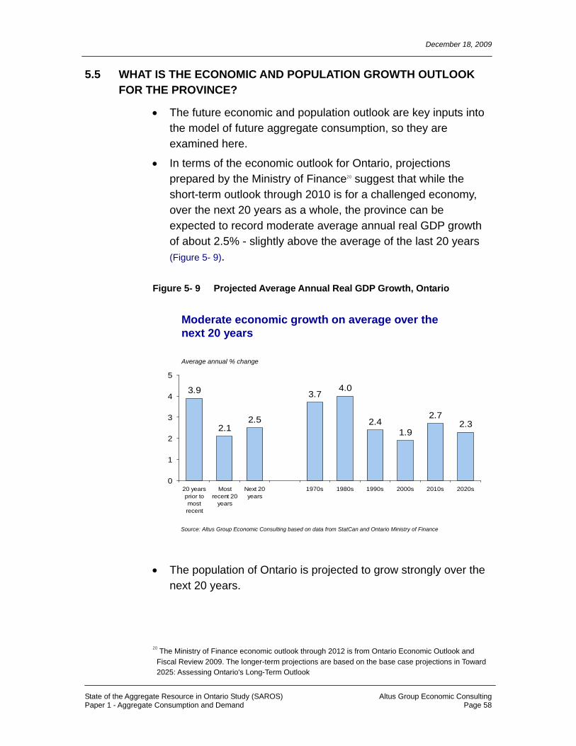
December 18, 2009


5.5 WHAT IS THE ECONOMIC AND POPULATION GROWTH OUTLOOK FOR THE PROVINCE?

• The future economic and population outlook are key inputs into the model of future aggregate consumption, so they are examined here.

• In terms of the economic outlook for Ontario, projections prepared by the Ministry of Finance20 suggest that while the short-term outlook through 2010 is for a challenged economy, over the next 20 years as a whole, the province can be expected to record moderate average annual real GDP growth of about 2.5% - slightly above the average of the last 20 years (Figure 5- 9).

Figure 5- 9 Projected Average Annual Real GDP Growth, Ontario

Moderate economic growth on average over the next 20 years

3.9

2.12.5

3.74.0

2.41.9

2.72.3

0

1

2

3

4

5

20 yearsprior tomostrecent

Mostrecent 20

years

Next 20years

1970s 1980s 1990s 2000s 2010s 2020s

Average annual % change

Source: Altus Group Economic Consulting based on data from StatCan and Ontario Ministry of Finance

• The population of Ontario is projected to grow strongly over the

next 20 years.

20 The Ministry of Finance economic outlook through 2012 is from Ontario Economic Outlook and Fiscal Review 2009. The longer-term projections are based on the base case projections in Toward 2025: Assessing Ontario's Long-Term Outlook

December 18, 2009


• Projections prepared by the Province21 suggest that Ontario’s population will grow by about 150,000 persons per year on average over the next 20 years – similar to the past 20 years (Figure 5- 10) – for total growth for the period of about 3 million persons.

Figure 5- 10 Projected Average Annual Total Population Growth, Ontario

Ontario is expected to continue to add about 150,000 people a year

123149 150

102

144 140157 149 151

0

40

80

120

160

200


Mostrecent 20

years

Next 20years

1970s 1980s 1990s 2000s 2010s 2020s

Average annual persons, 000s


• The rate of population growth however – which measures absolute growth against the size of the existing population base – will be gradually declining over the projection period (Figure 5- 11).

• In terms of the number of people, growth will continue to be focused in the GTA (Figure 5- 12).22

21 For the disaggregation by geographic area, the projections from the Growth Plan for the Greater Golden Horseshoe have been adopted (which are based on the compact growth scenario); for other areas of the province, the 2009 Ministry of Finance projections are used. The province totals are the sum of the projections for the GGH and other areas.

22 Projections of total population for Ontario and by geographic area are provided in Appendix A.

December 18, 2009


Figure 5- 11 Projected Average Annual Population Growth Rate, Ontario

Ontario’s rate of population growth will be declining

1.4 1.3

1.01.2

1.6

1.3 1.31.1 1.0

0.0

0.4

0.8

1.2

1.6

2.0


Mostrecent 20

years

Next 20years

1970s 1980s 1990s 2000s 2010s 2020s

Average annual % change


Figure 5- 12 Share of Future Population Growth by Geographic Area

The GTA expected to continue to account for the largest share of population growth

11 9 11

47

412

3 37 7

17

56

310

1 0

-15

0

15

30

45

60

75

Southwest

Penin-sula

WestCentral

GTA EastCentral

East North-east

North-west

Share of total population2009Share of populationgrowth next 20 years

%


December 18, 2009


• However the West Central area is expected to grow faster in relative terms than the GTA, and the other geographic areas (Figure 5- 13).

Figure 5- 13 Projected Population Growth Rate, Geographic Areas

West Central population growth expected to be stronger than the GTA in relative terms

0.7 0.7

1.8 1.8

0.91.1

-0.1-0.3

1.3

0.60.8

1.6

1.2

0.70.9

0.2

-0.1

1.0

-1.0

-0.5

0.0

0.5

1.0

1.5

2.0

2.5

3.0

Southwest

Penin-sula

WestCentral

GTA EastCentral

East North-east

North-west

Ontario

Past 20 yearsNext 20 years

Population growth, average annual %

Source: Altus Group Economic Consulting based on data from Statistics Canada and Ontario Ministry of Finance

5.6 WHAT IS THE PROJECTED TREND IN PER CAPITA AGGREGATE CONSUMPTION?

• Based on the economic and population growth scenario outlined it the previous section, as well as assumptions on future housing starts and the unemployment rate,23 an initial projection of per capita aggregate consumption was derived using the regression model outlined earlier.

• This initial projections (Figure 5- 14) showed lower average per capita consumption of aggregate in the next 20 years (12.6 tonnes per capita) compared to the most recent 20 years (which was 14.0 tonnes per capita).

23 While not shown here, the other required inputs for the regression model are housing starts and the unemployment rate; these inputs are provided in Appendix A.

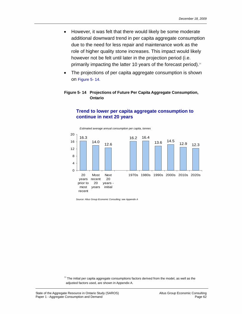
December 18, 2009


• However, it was felt that there would likely be some moderate additional downward trend in per capita aggregate consumption due to the need for less repair and maintenance work as the role of higher quality stone increases. This impact would likely however not be felt until later in the projection period (i.e. primarily impacting the latter 10 years of the forecast period).24

• The projections of per capita aggregate consumption is shown on Figure 5- 14.

Figure 5- 14 Projections of Future Per Capita Aggregate Consumption, Ontario

Trend to lower per capita aggregate consumption to continue in next 20 years

16.314.0

12.6

16.2 16.413.6 14.5

12.9 12.3

0

4

8

12

16

20

20years

prior tomost

recent

Mostrecent

20years

Next20

years -initial

1970s 1980s 1990s 2000s 2010s 2020s


Source: Altus Group Economic Consulting; see Appendix A

24 The initial per capita aggregate consumptions factors derived from the model, as well as the adjusted factors used, are shown in Appendix A.

December 18, 2009


5.7 WHAT IS THE PROJECTED CONSUMPTION OF AGGREGATE IN ONTARIO OVER THE NEXT 20 YEARS?

• The projections of per capita aggregate consumption were applied to the projections of total population outlined in Section 5.5 to derive the projections of total aggregate consumption over the next 20 years. 25

• Ontario can be expected to consume in the order of 186 million tonnes of aggregate per year on average over the next 20 years, both primary and secondary combined (Figure 5- 15).26 This is above the average level of the last 20 years as a whole.

Figure 5- 15 Average Annual Projected Total Aggregate Consumption, Ontario

Ontario’s consumption of aggregate expected to be higher over the next 20 years than the last 20 years

144164

186

134154 148

179 180 191

0

40

80

120

160

200


Mostrecent 20

years

Next 20years

1970s 1980s 1990s 2000s 2010s 2020s

Average annual aggregate consumption, millions of tonnes


25 More detail on the projection inputs and outputs, as well as 5 year intervals, are provided in Appendix A.

26 As indicated earlier, a construction expenditures/input factors approach (similar to that used in the 1992 State of the Resources Study) was used to confirm the reasonableness of the projections generated through the per capita methodology adopted for the current study. The alternate approach generated total aggregate consumption of between 180 and 190 million tonnes per year on average over the next 20 years (compared to the 186 million tonnes average using the per capita methodology).

December 18, 2009


• Note that the projections of future aggregate use should be viewed as being an “unconstrained” scenario. In particular, the projections assume that:

− Increases in the future price of aggregate are more or less in line with general price increases in the economy (i.e. that aggregate prices do not experience any more substantial upward “shocks” that could impact underlying consumption patterns)

− Sufficient aggregate is available to meet the expected underlying consumption patterns

• Consumption of aggregate in the GTA is expected to be moderately higher in the next 20 years compared to the most recent 20 years, and will continue to account for roughly one-third of the province’s total aggregate use (Figure 5- 16).

Figure 5- 16 Projected Total Aggregate Consumption by Geographic Area

Most areas of the province expected to consume at least as much aggregate in the next 20 years as the last 20 years

2116 18

54

8

23

12 11

2117

24

61

9

29

1510

0

15

30

45

60

75

Southwest

Penin-sula

WestCentral

GTA EastCentral

East North-east

North-west

Last 20 yearsNext 20 years


Source: Altus Group Economic Consulting, see Appendix A

• Most other areas of the province also will have higher average aggregate consumption levels than in the past 20 years, except for the Southwest and the Northwest.

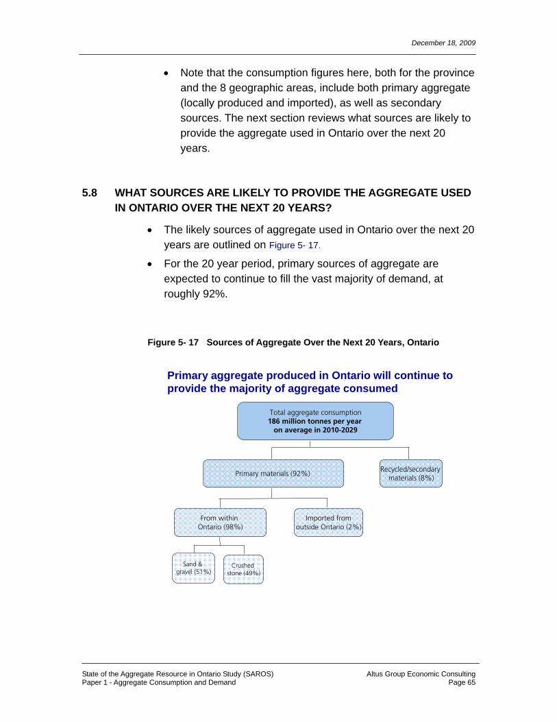
December 18, 2009


• Note that the consumption figures here, both for the province and the 8 geographic areas, include both primary aggregate (locally produced and imported), as well as secondary sources. The next section reviews what sources are likely to provide the aggregate used in Ontario over the next 20 years.

5.8 WHAT SOURCES ARE LIKELY TO PROVIDE THE AGGREGATE USED IN ONTARIO OVER THE NEXT 20 YEARS?

• The likely sources of aggregate used in Ontario over the next 20 years are outlined on Figure 5- 17.

• For the 20 year period, primary sources of aggregate are expected to continue to fill the vast majority of demand, at roughly 92%.

Figure 5- 17 Sources of Aggregate Over the Next 20 Years, Ontario

Total aggregate consumption186 million tonnes per year

on average in 2010-2029

Primary materials (92%)

From within Ontario (98%)

Imported fromoutside Ontario (2%)

Recycled/secondary materials (8%)

Sand & gravel (51%)

Crushed stone (49%)

Primary aggregate produced in Ontario will continue to provide the majority of aggregate consumedPrimary aggregate produced in Ontario will continue to provide the majority of aggregate consumed

December 18, 2009


• The vast majority of primary aggregate (98%) is expected to continue to be supplied from Ontario operations – suggesting Ontario’s primary production will be about 171 million tonnes a year, up from an average of 154 millions tonnes per year in the most recent 20 years.

• Secondary products (primarily recycling) are expected to be an increasing source of supply, averaging about 8% of the total aggregate consumed for the next 20 years as a whole (but increasing to about 9% in the 2020s).27

• For the geographic areas, estimates of regional exchanges of aggregate based on trends in the 2000s were used to determine what the likely level of locally produced primary aggregate would be. Note that these estimates are based on recent trends – assuming the “status quo” in terms of no additional supply side constraints.

• The estimates suggest that the GTA is likely to continue to be a net importer of aggregate, with the main source the neighbouring geographic areas (Figure 5- 18).

• As discussed earlier, there is expected to be a continued gradual shift in Ontario towards the use of higher quality crushed stone.

• The contribution of crushed stone to the supply of total primary aggregate consumed in each geographic area over the next 20 years is shown on Figure 5- 19.

27 Discussions with LVM-Jegel suggest that the additional penetration based on existing capabilities would likely not exceed 10% of total aggregate consumed.

December 18, 2009


Figure 5- 18 Local Primary Production of Aggregate Compared to Total Consumption of Aggregate, Geographic Areas

GTA expected to continue to consume aggregate produced by neighbouring areas

1813

38

29

19

28

1610

2117

24

61

9

29

1510

0

15

30

45

60

75

Southwest

Penin-sula

WestCentral

GTA EastCentral

East North-east

North-west

Local primary productionTotal consumption*

Estimated average annual, millions of tonnes


* As filled by all sources – local primary production, international and interregional imports and secondary sources

Figure 5- 19 Crushed Stone as % of Total Consumption of Primary Aggregate, Geographic Areas

Usage of crushed stone expected to continue to increase

18

72

17

45 43

70

25

12

41

26

80

25

53 50

78

32

19

49

0

20

40

60

80

100

Southwest

Penin-sula

WestCentral

GTA EastCentral

East North-east

North-west

Ontario

Last 10 yearsNext 20 years

Estimated average annual, %


December 18, 2009


5.9 WHAT ALTERNATE SCENARIOS SHOULD BE CONSIDERED?

• The projections presented in the previous section are based on the Province’s most recent “base case” economic and population scenarios, which are consistent with a medium growth scenario.

• At the Ontario level only, alternate projections that represent low and high growth scenarios were also formulated.28

• The resulting projections show a range of potential aggregate consumption over the next 20 years, from a low of about 161 million tonnes per year on average to a high of about 223 million tonnes per year (Figure 5- 20).29 It can be noted, however, that even under the low scenario, future aggregate consumption would not be lower than in the most recent 20 years.

Figure 5- 20 Alternate Scenarios of Future Aggregate Consumption, Ontario

Even under a low growth scenario, Ontario would continue to use as much aggregate as past 20 years

161144

164186

223

0

50

100

150

200

250

20 years prior to most recent Most recent 20 years Next 20 years

Low scenario Medium "base" scenario High scenario



28 The alternate scenarios were not produced for the geographic areas, as low and high population projections are not prepared below the Ontario-wide level.

29 More details for the alternate projection scenarios are provided in Appendix A.

December 18, 2009


6.0 KEY FINDINGS AND SUGGESTIONS FOR FUTURE WORK This section summarizes some of the key findings of the analysis, and outlines areas of the analysis that could benefit from additional work.

6.1 KEY FINDINGS

This section summarizes the key findings of the paper.

6.1.1 Ontario’s aggregate consumption patterns

• Over the past 20 years, Ontario has consumed over 3 billion tonnes of aggregate - or about 164 million tonnes per year on average.

• On a per capita basis, about 14 tonnes of aggregate were consumed each year in the past 20 years – down from about 16 tonnes per capita in the previous 20 years. The highest per capita consumption of aggregate is in Northern Ontario, the lowest in the GTA.

• The aggregate that Ontario uses comes mainly from primary sources of material extracted from Ontario pits and quarries. Imports from other countries play only a small role. Secondary sources of material (primarily recycled materials) have played an increasing role, at about 7% of consumption in the past 10 years (up from about 4% in the early 1990s).

• Most parts of the province saw some increase in consumption of aggregate during the 2000s compared to the 1990s – even those where population growth declined, or was negative. This illustrates the point that while growth is an important driver of the use of aggregate, there is also demand generated from within the existing population base.

• For most of the 8 geographic areas of the province considered in this study, the aggregate consumed mainly comes from primary and secondary aggregate produced locally within those areas. However, that is not the case for the GTA, which imports about half of the aggregate it uses from neighbouring areas

• Both sand and gravel, and crushed stone, are used. Crushed stone currently accounts for less than half of the primary aggregate consumed, but its share has been increasing.

December 18, 2009


6.1.2 Aggregate consumption in Ontario compared to other areas

• Available data suggests that Ontario’s per capita consumption of aggregate is broadly similar to other provinces but somewhat higher than western European countries (except for Ireland and Finland), Australia, New Zealand and the U.S, although the degree of the difference is not conclusive given data comparability issues.

• Factors which likely contribute to lower per capita aggregate consumption in European countries compared to Ontario include:

− Being more densely populated than Ontario

− Having slower rates of population growth than Ontario

− Have slightly lower rates of GDP growth than Ontario over the period examined and slightly lower GDP per capita

− Having somewhat higher mean temperatures than Ontario

− Having higher rates of use of secondary aggregate than Ontario.

6.1.3 The ways in which aggregate is used in Ontario

• Aggregate is used for a wide range of applications, however the primary use is in construction work - either directly, or through concrete and other building products.

• Roads (provincial highways, as well as municipal and private roads) account for the largest share of construction-related aggregate, at about one-half.

• The amount of aggregate used per dollar of construction spending has been on a generally downward trend since the early 1980s.

• Some examples of typical amounts of aggregate used in various applications include:

− 18,000 tonnes per kilometre of 2 lane highway

December 18, 2009


− 250 tonnes for a 185 m2 house

− 114,000 tonnes per kilometre of a subway line

6.1.4 The future consumption of aggregate in Ontario

• Based on provincial government projections, Ontario is expected to continue to experience substantial economic and population growth over the next 20 years.

• This growth will generate the need for aggregate for construction work and other applications - on average, about 186 million tonnes per year (or roughly 3.7 billion tonnes in total), above the levels of the past 20 years.

• While some moderate increase is expected in the share of aggregate consumption filled by recycled materials, the main source is expected to continue to be primary aggregate from Ontario pits and quarries (an average of roughly 171 million tonnes per year compared to 154 million tonnes per year over the past 20 years).

• The GTA, and broader Greater Golden Horseshoe, are expected to use more aggregate over the next 20 years than in the past 20 years.

6.2 SUGGESTIONS FOR FUTURE WORK

• The estimates of sources of aggregate supply for the geographic areas prepared for this study required the formulation of assumptions about the extent of movements of aggregate within the province. The internal “trade” estimates for this study were derived based on a combination of methods, including examination of construction activity over the past 10 years, an analysis of local production patterns relative to growth patterns to see what “excesses” are being generated and then potentially exported to other areas, as well as discussions with key industry participants. The analysis however is not definitive, and could benefit from a formal survey process undertaken on a periodic basis (similar to that conducted in the UK), to establish movements of aggregate within the province. Such an

December 18, 2009


undertaking would require the buy-in and support of the provincial government, as well as the aggregates industry and also major purchasers of aggregate to determine where these consumers obtain their supplies (since producers do not necessarily know the end destination for their products).

• In addition, research by LVM-Jegel suggests that recycled material currently fills roughly 7% of aggregate supply on a province-wide basis, and that the proportion is likely higher in the GTA and major urban areas, and lower in smaller centres. Additional research to better understand the variation in use of recycled material by geographic area in the province would be beneficial to the projection exercise.

• An initial thought piece on the potential impact of various development patterns and trends was undertaken for this study by MHBC Planning, which showed that there are a myriad of factors which could potentially impact future aggregate consumption per capita – some increasing and some decreasing. Further work in this area to quantify some of these impacts would be beneficial in the projection exercise, in particular to differentiate between short-term and long-term impacts, and between per capita needs for new development versus on-going maintenance and repair.

• It is recommended that the projections of aggregate consumption be monitored on a periodic basis (such as every other year) to see how they are tracking, as well as to incorporate relevant updated projections of economic and population growth.

December 18, 2009


List of References British Geological Survey, 2008, European Mineral Statistics 2002-06, Keyworth, Nottingham; British Geological Survey.

British Geological Survey, 2008, United Kingdom Minerals Yearbook 2007, Keyworth, Nottingham; British Geological Survey.

British Geological Survey, 2009, European Mineral Statistics 2003-07, Keyworth, Nottingham; British Geological Survey,).

British Geological Survey, 2008, Managing Aggregates Supply in England, Keyworth, Nottingham; British Geological Survey.

Canada Mortgage and Housing Corporation, Housing Time Series database.

Canadian Urban Institute, Between Rock and a Hard Place: Understanding the Foundations of Ontario’s Built Future.

Chang, I-Cheng & Hsiao, Teng-Yuan (2004), Short-Term Model of the Production of Construction Aggregates in Taiwan Based on Artificial Neural Networks.

Clayton Research Associates Limited, The Demand for Aggregate in Ontario: The Outlook Through 2010, January 1996.

Coriolis Consulting Group (1996), Development of a Model for Forecasting the Consumption of Aggregates in the Lower Mainland, Ministry of Energy, Mines and Petroleum Resources, October 1996.

Coulter, Terence (2003), Changes in Aggregate Production and Use in Victoria B.C.

Hemson Consulting Ltd., The Growth Outlook for the Greater Golden Horseshoe, January 2005.

Johansson, Kurt et al (2008), Industrial Minerals and Rocks, Aggregates and Natural Stones in the Nordic Countries.

Karakas, Ahmet & Turner, Keith (2004), Aggregate Supply and Demand Modeling Using GIS Methods for the Front Range Urban Corridor, Colorado.

Kohler, Susan (2006), Aggregate Availability in California, California Department of Conservation, California Geological Survey.

December 18, 2009


Koziol, Wieslaw et al (2008), Production of Aggregates in European Union.

Matten, E. E. (1982), A Simplified Procedure for Forecasting Demand for Mineral Aggregate in Ontario - Industrial Mineral Background Paper 4, Ontario Ministry of Natural Resources, March 1982.

Metrolinx (2008), The Big Move: Transforming Transportation in the Greater Toronto and Hamilton Area, Greater Toronto Transportation Authority.

Minister of Finance (2009), 2009 Ontario Budget: Budget Papers, Queen’s Printer for Ontario.

Minister of Finance (2009), 2009 Ontario Economic Outlook and Fiscal Review, Background Papers, Queen’s Printer for Ontario.

Nasser, Khalil (1987), Supply/Demand Analysis of Aggregates in the Denver Metro Area, Jefferson County, Colorado Planning & Zoning Department.

NZIER (2008), Economic Analysis of the Quarrying and Aggregate Production Industry, Aggregate & Quarry Association of New Zealand.

O’Brien, J. (2006), Planning for Growth? The Determinants of Aggregates Demand in New Zealand.

Ontario Ministry of Finance (2005), Toward 2025: Assessing Ontario’s Long-Term Outlook, Queen’s Printer for Ontario.

Ontario Ministry of Finance, Fall 2009, Ontario Population Projections, 2008-2036, Queen’s Park Printer for Ontario 2009.

Ontario Ministry of Municipal Affairs and Housing, Greenbelt Plan 2005, Queen’s Printer for Ontario, February 28, 2005.

Ontario Ministry of Northern Development and Mines, Ontario Mineral Score, Government of Ontario.

Ontario Ministry of Public Infrastructure Renewal, Places to Grow; Growth Plan for the Greater Golden Horseshoe, 2006, Queen’s Printer for Ontario, 2006.

Ontario Ministry of Transportation, Transportation Fact Sheet (Various), July 28, 2008.

December 18, 2009


Organization for Economic Co-operation and Development, OECD Database (2008), Gross domestic product (expenditure approach), US $, current prices, 22 July 2009, OECD.

Peat, Marwick and Partners & M. M. Dillon Limited (1980), Mineral Aggregate Transportation Study – Industrial Mineral Background Paper 1, Ministry of Natural Resources, December 1980.

Planning Initiatives Ltd. and Associates, Aggregate Resources of Southern Ontario: A State of the Resource Study, November 1992.

Proctor & Redfern Limited (1974), Mineral Aggregate Study of the Central Ontario Planning Region, Ministry of Natural Resources, March 1974.

Robinson, Gilpin & Brown, William, Sociocultural Dimensions of Supply and Demand for Natural Aggregate – Examples from the Mid-Atlantic Region, United States, United States Geological Survey.

Statistics Canada, 2005 Input-Output Model Simulations (National Model), Statistics Canada Catalogue no. 15F0004XDB.

Statistics Canada, 2008, Implicit Price Indexes, Gross Domestic Product (table), Provincial and Territorial Economic Accounts Review, 2008, Statistics Canada Catalogue no. 13-016-X.

Statistics Canada, 2008, Real Gross Domestic Product, Expenditure-based (table), Provincial and Territorial Economic Accounts Review, 2008, Statistics Canada Catalogue no. 13-016-X.

Statistics Canada, 2009, Cd1T30an Labour Force Estimates by Provinces, Territories and Economic Regions, annual average (table), Labour Force Historical Review, 2008, Statistics Canada Catalogue no. 71F0004XCB.

Statistics Canada, Annual Population Estimates for July 1, 1971 to 2008, Canada, Provinces and Territories (table), Annual Demographic Statistics, 2008, Statistics Canada Catalogue no. 91-213-XIB.

Statistics Canada, Non-metallic Mineral Mining and Quarrying NAICS 2123, 2006, Statistics Canada Catalogue no. 26-226-X.

December 18, 2009


Statistics Canada, Table 026-0013 Residential values, by type of investment, quarterly (dollars), CANSIM (database).

Statistics Canada, Table 026-0016 Investment in non-residential building construction, by type of building, province and census metropolitan area (CMA), quarterly (dollars), CANSIM (database).

Statistics Canada, Table 026-009 Maintenance and repair expenditures in housing, annual (dollars), CANSIM (database).

Statistics Canada, Table 029-0002 Capital expenditures on construction, by type of asset, annual (dollars). CANSIM (database).

Statistics Canada, Table 029-0040 Capital expenditures on construction, by type of asset, annual (dollars), CANSIM (database).

Statistics Canada, Table 031-0002 Flows and stocks of fixed non-residential capital, by North American Industry Classification System (NAICS) and asset, Canada, provinces and territories, annual (dollars), CANSIM (database).

Statistics Canada, Table 032-0002 Public and private investment, summary by province and territory, annual (dollars), CANSIM (database).

Statistics Canada, “Value of Non-Residential Building Permits by Municipality, Greater Toronto Area & Kitchener CMA” (table), Building Permits, Statistics Canada Catalogue no. 64-001-XWF.

The Australian Quarrying Industry – Industry Analysis, www.quarry.com.

The Ontario Aggregate Resources Corporation (1998 - 2008), Mineral Aggregates in Ontario, Production Statistics.

U.S. Bureau of Economic Analysis, Gross Domestic Product by State in Current and Real (2000) Dollars by State, Table 649, June 2008.

U.S. Bureau of Economic Analysis, Survey of Current Business, July 2008.

U.S. Census Bureau, 2008 Population Estimates by State, Table 3, Population Estimates Program.

December 18, 2009


U.S. Geological Survey, Department of the Interior/USGC, Minerals Yearbook, Sand and Gravel (1994-2007).

U.S. Geological Survey, Department of the Interior/USGC, Minerals Yearbook, Silica (1994-2007).

U.S. Geological Survey, Department of the Interior/USGC, Minerals Yearbook, Stone, Crushed (1994-2006).

U.S. Geological Survey, Department of the Interior/USGC, Minerals Yearbook, Stone, Dimension (1994-2007).

SAROS Paper 1 - Aggregate Consumption and Demand

Appendix AProjection Model Background

Altus Group Economic ConsultingDecember 2009

December 18, 2009

A- 2

Table of Contents Summary of Previous Aggregate Forecasting Models Prepared for MNR Page A-3 Summary of Aggregate Forecasting Models for Other Areas Page A-7 Outline of SAROS Paper 1 Projection Methodology Page A-19 Key SAROS Paper 1 Model Tables Page A-20

December 18, 2009

A- 3

Summary of Previous Aggregate Forecasting Models Prepared for MNR

MNR has commissioned a number of studies over the years which included methodologies to forecast the use of aggregates. Mineral Aggregate Study: Central Ontario Planning Region This study of aggregates in the Central Ontario Planning Region was undertaken by Proctor and Redfern in 1974. The demand modelling part of the exercise was based on projecting the future value of different types of construction expenditures (residential construction, non-residential building and total engineering - both road and non-road) and applying "input factors" i.e. the tonnes of aggregate used per $1,000 ($1971) spent on each type of construction. The input factors were derived from an analysis of Statistics Canada's input-output model for 1971. Separate factors for direct usage of sand and gravel and crushed stone versus indirect usage of aggregate (i.e. in concrete products and ready-mix) were made. The projections of future construction spending for Ontario incorporated the following methodology:

Project real gross provincial product (GPP) per capita, then multiply by projected population to obtain total real GPP. Based on historical trends, project which proportion of GPP would be construction spending. Based on historical proportions, project the breakdown of total construction into each type of construction used in the model. Apply factors for each of sand and gravel and crushed stone to the projections of construction spending by type; sum up the

results to obtain total demand for aggregates. As part of the methodology, a share of total Ontario construction spending was apportioned to the Central Ontario Planning Region based on its share of population and relative growth rates. The methodology used to break down total construction by type in the Central Ontario Planning Region was similar to that for Ontario. The basic methodology for the projections provides a sound working framework, however, there were a few limitations:

There is no account made of aggregate used in non-construction purposes. The upfront assumption that the proportion of total construction accounted for by each type of construction will remain

constant over the projection period is of concern; although being more difficult, projecting each type of construction separately would seem to be preferable, given the different intensity of aggregate usage in varying types of construction.

The study recognizes that road construction is the single largest consumer of aggregates and actually presents separate input factors for road versus other types of engineering construction. However, in preparing the projections, road spending is

December 18, 2009

A- 4

combined with all other types of engineering spending, to which an overall input factor for all engineering is applied. Because the input factors are very different for road versus non-road construction, any changes in the mix of construction spending between road and other engineering in the future will not be translated into varying demand for aggregates.

Mineral Aggregate Transportation Study This study was undertaken by Peat Marwick and M.M. Dillon in 1980. The model produced for the study uses a combination of input factors/construction spending and regression analysis to project demand for aggregates in Ontario and four sub-areas: Toronto, London, Windsor and Chatham. Use of aggregates was projected separately for each of the following categories:

Concrete and products: usage in concrete was projected by directly relating it to real gross domestic product (GDP) with regression analysis.

Roads: MTO forecasts of road spending were used and projected ahead; input factors were then applied to these forecasts. Residential construction: projections of population by age and assumptions on average household size and housing type

preferences were used to project housing starts by type; usage factors per unit were then applied to these unit projections. These factors excluded aggregates used in concrete and concrete products, which were already accounted for in the overall concrete and concrete products projections.

Non-residential building, non-road engineering and all other uses: these projections were also derived based on regression analysis, related to GDP and excluded uses in concrete and concrete products.

The main limitation of the model is that it is somewhat complicated; as such, it does not lend itself to regular updates. A Simplified Procedure for Forecasting Demand for Mineral Aggregates in Ontario This study was prepared under the direction of E.E. Matten of the Ministry of Natural Resources in 1982. The object of the study was to be able to project the demand for aggregate on a small area basis (i.e. by municipality) with relative ease. The model uses the construction expenditures and input usage factors approach. Road factors were derived specifically for the study based on an analysis by MTO; factors for other types of construction spending were as derived based on information in regional studies of the aggregate industry.

December 18, 2009

A- 5

The first step in the forecasting process involved projecting Ontario total construction expenditures - this was done in relation to projections of real GDP. Then two scenarios of the distribution of total construction by type were made, one based on the historical share from 1971-1978, the other by extending the trend for that period. Sub-provincial areas were forecast based on an assessment of "regional pull" - this was based on an analysis of trends in retail sales and disposable income per capita. As per the Proctor and Redfern study, the main shortcoming of this model is that it assumes upfront what the distribution of construction by type will be, rather than building up to total construction by forecasting the individual components. As such, there is no allowance for changes in the distribution of spending which may emerge over the forecast period. Aggregate Resources of Southern Ontario: A State of the Resource Study This study was undertaken in 1992 with by Planning Initiatives as lead consultant. Chapter 4 and Appendix 4a were contributed by Clayton Research (now Altus Group Economic Consulting, the consultants for SAROS Paper 1). The projections were prepared for Ontario and selected market areas for the 1990 to 2010 period (annual projections were prepared but the emphasis was on 5 year average annual numbers). The methodology used a construction input factors was the main approach to projecting future aggregate usage. Using Statistics Canada’s input-output model, “input usage” factors for sand and gravel and stone were generated. These were then applied to projections of construction spending by type of construction (new residential, new non-residential building, new road, new other engineering and repair road). The limitations of the projection methodology included the difficulty in obtaining reasonable historical and projected construction spending by type of construction, as well as maintaining the input factors constant over time (as subsequent history as shown that these factors (i.e. the amount of aggregate used per dollar of construction spending) have declined over time. Two regression models were also developed, once which incorporated macro economic variables (housing starts, real GDP, unemployment rate), and one which was based on total construction spending.

December 18, 2009

A- 6

The Demand for Aggregate in Ontario: The Outlook Through 2010 This analysis was undertaken by Clayton Research in 1996 as an update for MNR of the State of the Resource Study projections. The update was warranted as the downturn in the first half of the 1990s was much more severe that macroforecasters had been expecting when the 1992 study was conducted. It also incorporated more recent population projections prepared by the province.

December 18, 2009

A- 7

Summary of Aggregate Forecasting Models for Other Areas This section summarizes a number of aggregate forecasting models that have been prepared for other areas of the world. The specific references for each model are provided in the Reference list in the main report. Changes in Aggregate Production and Use in Victoria, BC

Model form Regression analysis forecast

Explanatory variable included

Population, annual growth rate, aggregate usage data

Timeframe Forecast of the next 20 years based on 1993-1997 usage data

Complexity of the model/Ease of updating

Easy

Disaggregation of results n.a.

In this paper, Coulter forecasts the average annual aggregate demand of aggregates in the Victoria area between 2002 and 2022. The author estimated an average aggregate demand of 7.8t/person/year based on 1993-1997 aggregate usage data and population statistics for the CRD during that period. With the number of current population and an estimated annual growth, then he projected the local aggregate demand for the period of 2002 to 2022. Pros: simple & easy to apply Cons: aggregate consumption per capita was determined based on only 5 year historical data and the result is less reliable.

December 18, 2009

A- 8

Lower Mainland Aggregates Study (Vancouver)

Model form a. Direct usage forecast

b. Regression analysis forecast


Direct usage forecast

‐ Historical annual consumption of aggregates (assumed historical production equals historical consumption)

‐ Units of different type of residential, different of utilities construction/maintenance and other urban development, Aggregate usage factors (tones of aggregate used for each unit)

Regression

‐ Dependent variable- aggregate consumption

‐ Independent variables - Demographic/macroeconomic factors (population growth, GDP, housing starts)

Timeframe Direct usage forecast: 1991-1994

Regression:

Over 10 year period from 1985-1995 were used to predict consumption between 1996-2021


Moderate

Disaggregation of results Direct usage forecast

‐ Estimated consumption are significantly lower than the actual figures for 1991-1993, method discarded

December 18, 2009

A- 9

Regression

‐ High degree of correlation between historical aggregate consumption and historical population growth (existing number of residents plus natural increase & new residents due to in-migration) were found

‐ Demand forecast by subarea with three scenarios (current trends continued, maintenance/no growth, and compact region scenario) was summarized for the year 1996-2021

Direct usage forecast and regression analysis approaches were undertaken to develop aggregate demand models in the study area. For direct usage model, a bunch of historical data (housing starts by type of residence, office & industrial space by type, construction projects) and aggregates usage factors corresponding to the users of aggregates by area were obtained. However, the results of this approach were significantly lower than the actual production figures for most testing years given inaccurate data inputs and factors. In regression analysis, aggregate consumption acted as the dependent variable and the demographic/macroeconomic factors (i.e. population growth, GDP, housing starts) were used as independent variables. Average production figures of 1983 and 1986 were used to replace the figures of year 1984 and 1985 which are extremely high. Also, 3 year rolling average annual aggregate production figures were used to replace the actual figures to further smooth data. Test found that a high degree of correlation between historical aggregate consumption and historic population growth (separating natural increase and in-migration). Based on the equation produced by regression analysis, demand forecast by sub-area under three alternative scenarios of different growth level were presented. Pros: Two different approaches were examined and for the direct usage model, type of construction projects was used to get more accurate result. Cons: Lack of high quality and reliable data: In the direct usage approach, a complete set reliable data was only available for 5 years. Historic data for annual production was used in the research instead of historic data of actual aggregate consumption. The aggregate production data is available for the study area on a total study area basis only, and is not broken down by the defined market sub-areas within the study area. Furthermore, 1995 is the only year for which a breakdown of total study area production by type of aggregate is available.

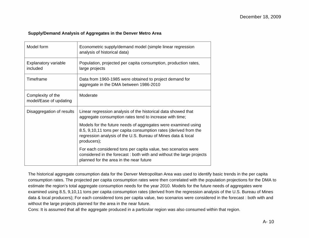
December 18, 2009

A- 10

Supply/Demand Analysis of Aggregates in the Denver Metro Area

Model form Econometric supply/demand model (simple linear regression analysis of historical data)


Population, projected per capita consumption, production rates, large projects

Timeframe Data from 1960-1985 were obtained to project demand for aggregate in the DMA between 1986-2010


Moderate

Disaggregation of results Linear regression analysis of the historical data showed that aggregate consumption rates tend to increase with time;

Models for the future needs of aggregates were examined using 8.5, 9,10,11 tons per capita consumption rates (derived from the regression analysis of the U.S. Bureau of Mines data & local producers);

For each considered tons per capita value, two scenarios were considered in the forecast : both with and without the large projects planned for the area in the near future

The historical aggregate consumption data for the Denver Metropolitan Area was used to identify basic trends in the per capita consumption rates. The projected per capita consumption rates were then correlated with the population projections for the DMA to estimate the region’s total aggregate consumption needs for the year 2010. Models for the future needs of aggregates were examined using 8.5, 9,10,11 tons per capita consumption rates (derived from the regression analysis of the U.S. Bureau of Mines data & local producers); For each considered tons per capita value, two scenarios were considered in the forecast : both with and without the large projects planned for the area in the near future. Cons: It is assumed that all the aggregate produced in a particular region was also consumed within that region.

December 18, 2009

A- 11

Aggregate Availability in California

Model form Per capita aggregate consumption forecast model


Historical production and population

Timeframe Data from 1960s -2005 used to predict California’s 50 year aggregate needs (2006-2055)


Easy

Disaggregation of results By subarea

‐ The Per Capita Consumption Model has proved to be effective for predicting aggregate demand in major metropolitan areas

‐ May not work well in county aggregate studies or in P-C regions that import or export a large percentage of aggregate resulting a low correlation between production districts and aggregate market areas. When this happens, projections are based on a historical production model where 50-year aggregate demand is determined by extending a best-fit line of historical aggregate production data for a county or region

This study compared 50-year aggregate demand and permitted resources for each area in California. A per capita aggregate consumption forecast model is used for aggregate demand projections. According to the researchers, population change is the only factor that showed strong correlation to historical aggregate use. Yearly historical production and population data from the 1960s through 2005 were obtained first. Annual historical per capita consumption was determined by dividing yearly aggregate production by the population for that same year. Then, projections of aggregate demand for a 50-year period were obtained by multiplying each year of projected population by the average historical per capita for a 50-year period from the beginning of 2006 through 2055.

December 18, 2009

A- 12

‐ Pros: simplicity and the availability of population data

‐ Cons: The random impacts of major public construction projects and economic recessions are assumed to be smoothed out over years; The years chosen to determine an average historical per capita consumption may differ depending upon historical aggregate use for that specific region; The projection model has proved to be effective in metropolitan areas, but may not work well in county aggregate studies or in P-C regions that import or export a larger percentage of aggregate resulting in a low correlation between production districts and aggregate market areas.

December 18, 2009

A- 13

Sociocultural Dimensions of Supply and Demand for Natural Aggregate – Examples from the Mid-Atlantic Region, United States

Model form Correlation analysis


Population density, size of planning area

Timeframe n.a.


Easy


A resource use model is derived based on population density and the size of the planning area. The larger the planning area, aggregate use fluctuates less as population densities increase than it would in a smaller planning area. Generally-speaking, the study finds that where there exists a population density of less than 1000 persons per square mile, production rates tended to be above the average production curve. Where there were more than 1000 persons per square mile, production rates fell below the average production curve. This is likely due to a variety of factors, including loss of available land, increased land costs, community opposition to industrial expansion, and other conflicting values. Pros:

o Simple model based on comparison of historical numbers

Cons:

o Authors cite this method of projection to be used for broad planning and projection purposes, and should be viewed as benchmark estimates with large uncertainties of approximately 25%.

o Despite mentioning the variety of factors that affect production rates as population densities change, there is no certainty provided through the model to determine the extent to which they are explanatory factors.

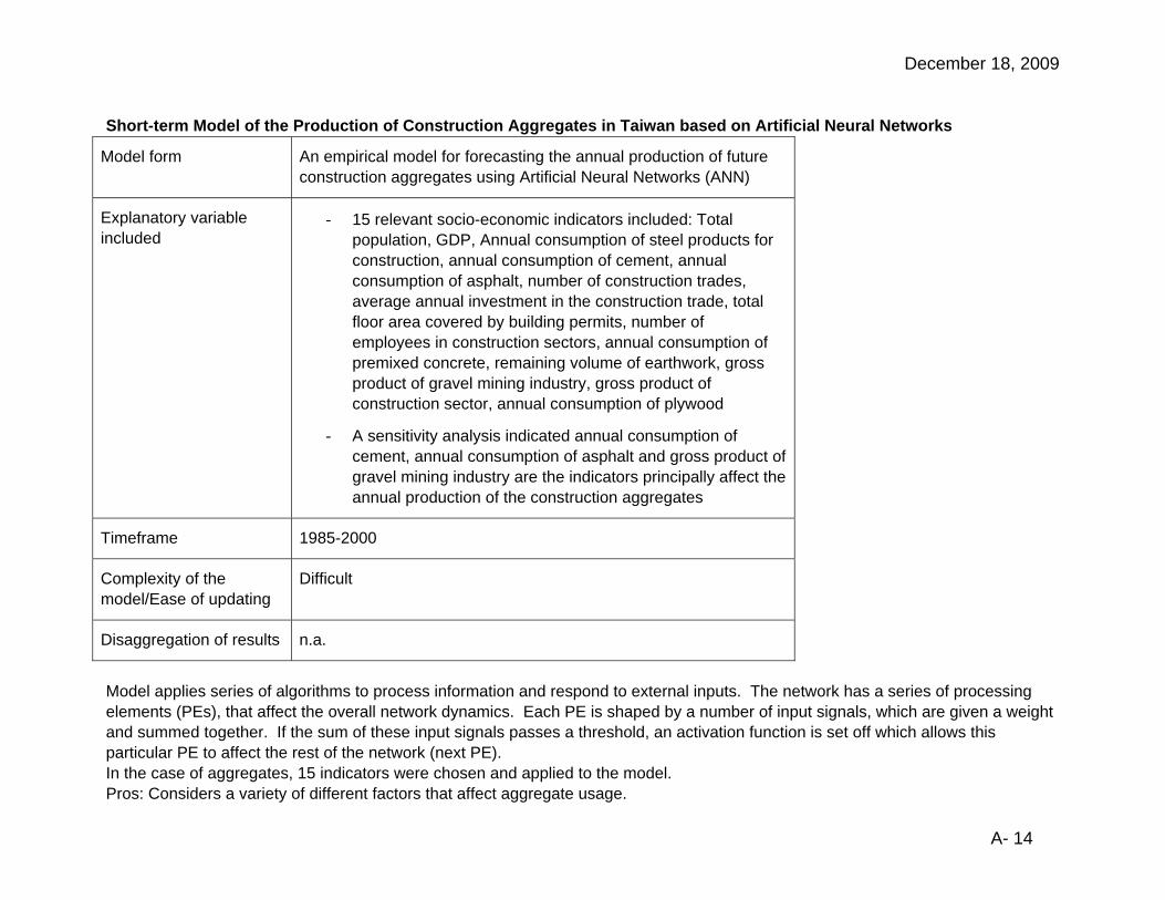
December 18, 2009

A- 14

Short-term Model of the Production of Construction Aggregates in Taiwan based on Artificial Neural Networks

Model form An empirical model for forecasting the annual production of future construction aggregates using Artificial Neural Networks (ANN)


‐ 15 relevant socio-economic indicators included: Total population, GDP, Annual consumption of steel products for construction, annual consumption of cement, annual consumption of asphalt, number of construction trades, average annual investment in the construction trade, total floor area covered by building permits, number of employees in construction sectors, annual consumption of premixed concrete, remaining volume of earthwork, gross product of gravel mining industry, gross product of construction sector, annual consumption of plywood

‐ A sensitivity analysis indicated annual consumption of cement, annual consumption of asphalt and gross product of gravel mining industry are the indicators principally affect the annual production of the construction aggregates

Timeframe 1985-2000


Difficult


Model applies series of algorithms to process information and respond to external inputs. The network has a series of processing elements (PEs), that affect the overall network dynamics. Each PE is shaped by a number of input signals, which are given a weight and summed together. If the sum of these input signals passes a threshold, an activation function is set off which allows this particular PE to affect the rest of the network (next PE). In the case of aggregates, 15 indicators were chosen and applied to the model. Pros: Considers a variety of different factors that affect aggregate usage.

December 18, 2009

A- 15

The Australian Quarrying Industry: Industry Analysis

Model form Time-series approach


Long term: historical consumption patterns, projected population levels (with time-series);

Short term: level of local economic growth and building and infrastructure development (annual demand varies from 6-10 tonnes per capita in different region)

Timeframe n.a.


Very brief


No actual model provided.

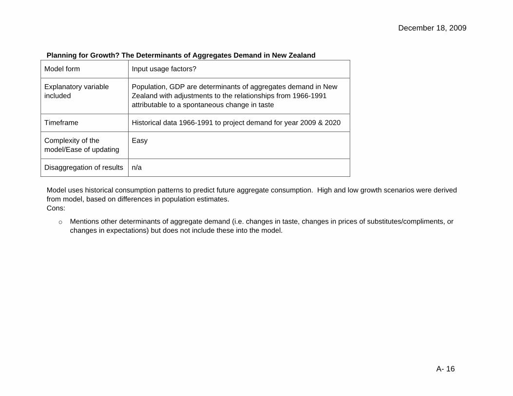
December 18, 2009

A- 16

Planning for Growth? The Determinants of Aggregates Demand in New Zealand

Model form Input usage factors?


Population, GDP are determinants of aggregates demand in New Zealand with adjustments to the relationships from 1966-1991 attributable to a spontaneous change in taste

Timeframe Historical data 1966-1991 to project demand for year 2009 & 2020


Easy

Disaggregation of results n/a

Model uses historical consumption patterns to predict future aggregate consumption. High and low growth scenarios were derived from model, based on differences in population estimates. Cons:

o Mentions other determinants of aggregate demand (i.e. changes in taste, changes in prices of substitutes/compliments, or changes in expectations) but does not include these into the model.

December 18, 2009

A- 17

Production of Aggregates in European Union

Model form Regression, Correlation, Artificial Neural Networks (ANN)


Aggregates production trends, consumption of aggregates and chosen economical growth indicators (mainly GDP), population or population density

Timeframe Data from 1991-2006 (varied by country) were used to predict production between 2007 and 2014


Easy

Disaggregation of results By country

Historical production/consumption patterns in the EU were analyzed using regression and correlation between GDP per capita and production per capita. Tests to determine linear relationships were conducted, as were other models to test for exponential, logarithmic, logistic, polynomial and other relationships. For analysis of individual countries, where regression and correlation could not be used, artificial neural network modeling was used to determine relationship between aggregate production per capita, GDP per capita, and population density. Pros:

o applies different models to determine relationship between production and GDP/population density

Cons:

o does not consider a host of other factors attributable to aggregate consumption

December 18, 2009

A- 18

Forecasting Aggregates Demand – A Technical Summary (UK)

Model form Regression-based approach


Construction activity (divided into low intensity of use & high intensity of use), aggregates levy, price change of different types of aggregates

Timeframe Total of 1980-1990, 1991-2000, forecast period 2000-2016


Moderate.

Disaggregation of results By region: Great Britain, Scotland, England and Wales, English sub-regions

The model focuses on construction activity as the main indicator in predicting aggregate usage, but groups different types of construction into two categories based on intensity of use – less aggregate intensive (industrial, commercial, housing repair, and other private repair) and more aggregates intensive (new housing, infrastructure, other new work (public), and other public repair). The model also employs another variable to capture the general reduction in aggregate intensity within the construction industry. Forecasts are derived at the national level by applying an annual growth rate of forecasted construction gross value added (supplied by Cambridge Econometrics) to historical construction data starting from the year 2000. The model is then applied to these forecasted aggregate numbers. When forecasting aggregate usage, the model attempts to capture other variables – particularly the aggregates levy and the subsequent change in prices for primary aggregates vs. alternative aggregates (since the latter are not taxed). Forecasts are then disaggregated based on 1999 consumption data. Pros: Considers a variety of factors that impact aggregate usage (i.e. intensity of use) and combines long-term changes in attitude/preference (trends) with other elements such as taxes to achieve a well-rounded outlook. Cons: Lack of data remains to be an issue; many assumptions made based on anecdotal evidence, so results can still be questioned.

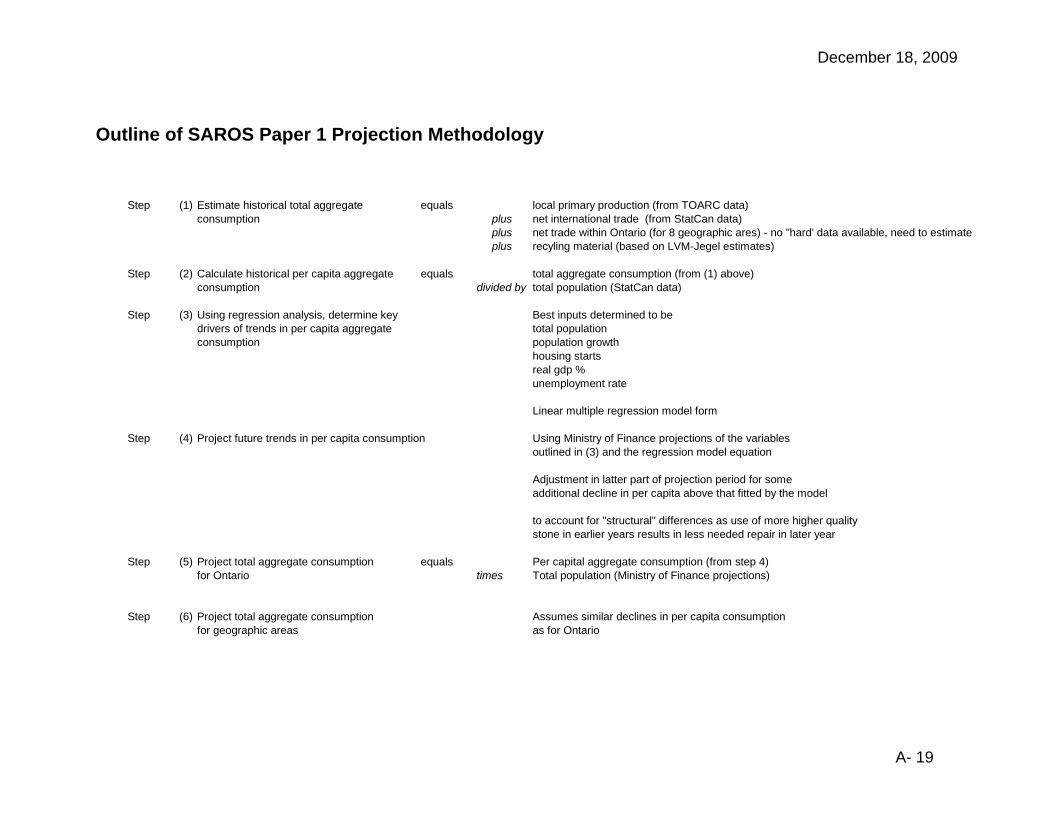
December 18, 2009

A- 19

Outline of SAROS Paper 1 Projection Methodology

Step (1) equals local primary production (from TOARC data)plus net international trade (from StatCan data)plus net trade within Ontario (for 8 geographic ares) - no "hard' data available, need to estimateplus recyling material (based on LVM-Jegel estimates)

Step (2) equals total aggregate consumption (from (1) above)divided by total population (StatCan data)

Step (3) Using regression analysis, determine key Best inputs determined to bedrivers of trends in per capita aggregate total populationconsumption population growth

housing startsreal gdp %unemployment rate

Linear multiple regression model form

Step (4) Project future trends in per capita consumption Using Ministry of Finance projections of the variablesoutlined in (3) and the regression model equation

Adjustment in latter part of projection period for someadditional decline in per capita above that fitted by the model

Step (5) Project total aggregate consumption equals Per capital aggregate consumption (from step 4)for Ontario times Total population (Ministry of Finance projections)

Step (6) Project total aggregate consumption Assumes similar declines in per capita consumptionfor geographic areas as for Ontario

Calculate historical per capita aggregate consumption

Estimate historical total aggregate consumption

to account for "structural" differences as use of more higher quality stone in earlier years results in less needed repair in later year

December 18, 2009

A- 20

Key SAROS Paper 1 Model Tables Table A.1 ANNUAL PRODUCTION OF PRIMARY AGGREGATE BY SOURCE AND COMMODITY TYPE, ONTARIO

Table A.2 ESTIMATED ANNUAL PRODUCTION OF PRIMARY AGGREGATES IN ONTARIO BY GEOGRAPHIC AREA

Table A.3 ESTIMATED LOCAL PRIMARY AGGREGATE PRODUCTION BY GEOGRAPHIC AREA AND COMMODITY TYPE

Table A.4a KEY AGGREGATE CONSUMPTION MODEL INPUTS AND OUTPUTS, BASE SCENARIO

Table A.4b KEY AGGREGATE CONSUMPTION MODEL INPUTS AND OUTPUTS, LOW SCENARIO

Table A.4c KEY AGGREGATE CONSUMPTION MODEL INPUTS AND OUTPUTS, HIGH SCENARIO

Table A.5 SOURCES OF AGGREGATE SUPPLY, ONTARIO

Table A.6

Table A.7

Table A.8 REGRESSION MODEL TO PROJECT PER CAPITA AGGREGATE CONSUMPTION

Table A.9 SUMMARY OF KEY MODEL INFORMATION SOURCES

Table A.10 INTERNATIONAL TRADE AGGREGATE RELATED HS CODES

POPULATION AND PER CAPITA PRODUCTION AND CONSUMPTION OF AGGREGATE BY GEOGRAPHIC AREA, ONTARIO

COMPARISON OF LOCAL PRIMARY PRODUCTION AND TOTAL LOCAL CONSUMPTION OF AGGREGATE BY GEOGRAPHIC AREA

December 18, 2009

A- 21

Table A.1ANNUAL PRODUCTION OF PRIMARY AGGREGATE BY SOURCE AND COMMODITY TYPE, ONTARIOMillions of Tonnes

Actual/Estimated1986 1987 1988 1989 1990 1991 1992 1993 1994 1995 1996 1997 1998 1999 2000 2001 2002 2003 2004 2005 2006 2007 2008

BY SOURCE:Licenced 128.0 149.0 153.9 154.3 134.8 107.3 100.7 104.9 113.4 108.6 114.3 124.3 123.7 130.5 145.5 145.1 141.2 142.9 149.8 148.6 151.6 157.6 153.6Wayside Permits* 6.0 5.0 4.8 3.7 2.6 1.8 2.0 2.0 2.0 2.4 2.0 0.5 1.6 1.0 0.6 0.2 0.3 0.3 0.1 1.1 0.3 1.2 0.1Aggregate Permits* 19.0 18.0 24.0 25.0 11.0 14.0 13.0 12.0 10.0 9.0 9.0 8.0 9.0 11.0 10.0 7.0 7.0 7.0 7.0 8.0 11.0 8.0 7.0Category 14 (Forest Industry) 0.0 0.0 0.0 0.0 0.0 0.0 0.0 0.0 0.0 0.0 0.0 0.0 0.0 2.0 3.0 3.0 4.0 3.0 4.0 4.0 4.0 4.0 4.0Private Land Non-Designated 12.0 13.0 14.0 14.0 12.0 12.0 12.0 12.0 11.0 10.0 11.0 11.0 11.0 12.0 12.0 12.0 12.0 12.0 12.0 12.0 12.0 2.0 2.0Total 165.0 185.0 196.7 197.0 160.4 135.1 127.7 130.9 136.4 130.0 136.3 143.8 145.3 156.5 171.1 167.3 164.5 165.2 172.9 173.7 178.9 172.8 166.7

BY COMMODITY TYPE:

LicensedSand & Gravel 77.4 88.6 91.7 95.3 79.6 64.2 58.0 59.7 62.5 58.3 62.5 69.0 68.8 72.9 80.1 79.7 79.1 80.3 83.3 82.6 84.5 85.2 81.3Crushed Stone 48.5 57.0 60.3 57.0 52.4 40.3 39.5 43.1 47.9 47.1 47.5 51.2 51.6 53.4 62.6 61.8 58.2 59.2 62.8 62.3 64.2 69.2 69.5Other 2.1 3.4 1.9 2.0 2.7 2.8 3.2 2.2 2.9 3.2 4.3 4.0 3.2 4.3 2.8 3.5 3.9 3.4 3.7 3.7 2.9 3.2 2.7Total 128.0 149.0 153.9 154.3 134.8 107.3 100.7 104.9 113.4 108.6 114.3 124.3 123.7 130.5 145.5 145.1 141.2 142.9 149.8 148.6 151.6 157.6 153.6

Wayside Permits/Aggregate Permits/Private Land Non-Designated (Estimated)Sand & Gravel 32.0 30.8 36.8 36.6 21.2 23.2 23.0 22.2 20.5 18.9 19.8 17.0 18.4 21.8 22.8 19.5 20.0 19.8 20.6 22.3 19.9 12.6 10.2Crushed Stone & other 5.0 5.2 6.0 6.0 4.4 4.6 4.1 3.8 2.5 2.5 2.2 2.6 3.2 4.1 2.8 2.7 3.3 2.5 2.5 2.8 7.4 2.6 2.9

Total 37.0 36.0 42.8 42.7 25.6 27.8 27.0 26.0 23.0 21.4 22.0 19.5 21.6 26.0 25.6 22.2 23.3 22.3 23.1 25.1 27.3 15.2 13.1

Total (Estimated)Sand & Gravel 109.5 119.4 128.6 131.9 100.9 87.4 81.0 81.9 83.0 77.2 82.3 86.0 87.2 94.7 102.9 99.3 99.1 100.1 103.8 104.9 104.4 97.7 91.6Crushed Stone & other 55.5 65.6 68.2 65.0 59.5 47.7 46.8 49.0 53.4 52.8 53.9 57.8 58.1 61.8 68.2 68.1 65.4 65.1 69.0 68.8 74.5 75.0 75.1

Total 165.0 185.0 196.7 197.0 160.4 135.1 127.7 130.9 136.4 130.0 136.3 143.8 145.3 156.5 171.1 167.3 164.5 165.2 172.9 173.7 178.9 172.8 166.7

Source: Altus Group Economic Consulting based on data from Ministry of Natural Resources and TOARC

December 18, 2009

A- 22

Table A.2ESTIMATED ANNUAL PRODUCTION OF PRIMARY AGGREGATES IN ONTARIO BY GEOGRAPHIC AREAMillions of Tonnes

Actual/Estimated1986 1987 1988 1989 1990 1991 1992 1993 1994 1995 1996 1997 1998 1999 2000 2001 2002 2003 2004 2005 2006 2007 2008

LicensedArea 1: Southwest 19.1 22.2 22.7 22.4 20.9 16.7 17.0 17.3 18.2 17.2 17.3 19.0 18.7 18.7 20.3 19.7 18.6 18.5 18.9 19.3 19.4 20.0 18.3Area 2: Peninsula 13.4 15.5 14.4 15.7 16.1 11.3 9.9 9.6 11.1 11.1 12.0 14.0 12.6 12.4 15.1 14.5 14.4 14.8 15.1 14.2 15.7 13.8 13.6Area 3: West Central 28.8 33.5 34.2 36.1 29.4 25.0 21.4 22.0 23.2 21.6 24.0 24.4 26.8 29.8 31.8 34.2 34.6 36.5 38.9 37.4 40.1 37.8 36.5Area 4: GTA 30.0 34.9 39.4 37.1 27.4 19.1 16.9 20.0 21.8 23.6 25.7 29.8 27.7 30.1 33.9 34.9 29.8 29.1 31.2 30.1 28.1 26.6 23.3Area 5: East Central 16.1 18.7 18.6 19.6 17.5 14.2 13.4 13.5 13.7 12.9 14.2 15.6 15.3 15.4 16.5 15.9 16.4 17.3 17.0 17.5 17.0 19.8 19.9Area 6: East 17.4 20.2 21.0 19.9 19.3 17.1 18.5 19.4 21.5 18.9 17.5 18.1 19.5 20.4 24.4 22.5 23.7 23.8 25.0 25.3 26.4 26.0 27.3Area 7: Northeast 2.5 2.9 2.8 2.4 3.5 3.3 3.2 2.7 3.4 2.9 3.0 2.8 2.5 3.0 2.7 2.8 2.9 2.3 2.8 3.6 3.7 10.4 11.1Area 8: Northwest 0.8 0.9 0.9 1.0 0.8 0.5 0.5 0.4 0.5 0.5 0.6 0.6 0.6 0.8 0.8 0.6 0.8 0.6 0.8 1.2 1.2 3.1 3.6Ontario 128.0 149.0 153.9 154.3 134.8 107.3 100.7 104.9 113.4 108.6 114.3 124.3 123.7 130.5 145.5 145.1 141.2 142.9 149.8 148.6 151.6 157.6 153.6

Wayside Permits/Aggregate Permits/Private Land/Category 14 (Estimated)Area 1: Southwest 1.4 1.2 1.0 1.0 0.8 0.7 0.1 0.6 0.5 0.5 1.5 0.0 0.0 0.0 0.1 0.0 0.0 0.0 0.0 0.0 0.0 0.3 0.0Area 2: Peninsula 0.1 0.1 0.1 0.1 0.2 0.2 0.1 0.3 0.5 0.3 0.0 0.3 0.0 0.0 0.0 0.0 0.1 0.2 0.1 0.0 0.2 0.0 0.0Area 3: West Central 1.7 1.4 1.2 1.2 0.9 0.6 1.2 0.9 1.3 0.8 0.5 0.2 0.3 0.4 0.2 0.2 0.1 0.1 0.0 0.1 0.1 0.0 0.1Area 4: GTA 1.4 1.2 1.3 0.7 0.4 0.1 0.1 0.1 0.0 0.0 0.0 0.1 0.0 0.1 0.0 0.0 0.0 0.0 0.0 0.0 0.0 0.0 0.0Area 5: East Central 2.1 2.0 2.2 2.0 1.6 1.3 1.6 1.5 1.7 1.4 1.5 1.5 1.8 2.0 1.8 1.6 1.9 1.8 1.6 1.7 1.9 0.2 0.1Area 6: East 2.8 2.9 3.1 3.0 2.8 2.6 2.6 2.5 0.6 1.3 0.0 0.1 1.7 1.7 0.3 0.1 0.2 0.4 0.0 0.3 0.1 0.4 0.1Area 7: Northeast 11.1 11.1 13.4 13.9 8.2 8.9 11.6 11.3 9.9 8.4 8.9 8.4 7.8 9.8 11.3 10.4 10.4 9.6 10.5 11.3 14.5 6.8 5.9Area 8: Northwest 16.4 16.1 20.4 20.9 10.8 13.4 9.7 8.8 8.6 8.7 9.6 9.0 10.0 12.0 11.9 9.8 10.7 10.3 10.9 11.7 10.5 7.4 6.9Ontario 37.0 36.0 42.8 42.7 25.6 27.8 27.0 26.0 23.0 21.4 22.0 19.5 21.6 26.0 25.6 22.2 23.3 22.3 23.1 25.1 27.3 15.2 13.1

Total (Estimated)Area 1: Southwest 20.5 23.4 23.8 23.4 21.7 17.4 17.1 17.9 18.7 17.7 18.8 19.0 18.7 18.7 20.4 19.7 18.6 18.5 18.9 19.4 19.4 20.3 18.3Area 2: Peninsula 13.5 15.6 14.5 15.8 16.3 11.5 10.1 9.9 11.5 11.4 12.0 14.3 12.6 12.4 15.1 14.5 14.5 15.0 15.2 14.2 15.9 13.9 13.6Area 3: West Central 30.5 34.9 35.4 37.3 30.3 25.6 22.6 22.8 24.6 22.4 24.4 24.6 27.1 30.2 32.1 34.4 34.7 36.7 39.0 37.5 40.2 37.8 36.5Area 4: GTA 31.4 36.1 40.7 37.8 27.7 19.2 17.0 20.1 21.8 23.6 25.7 29.9 27.7 30.2 33.9 34.9 29.8 29.1 31.2 30.1 28.1 26.6 23.3Area 5: East Central 18.2 20.7 20.8 21.5 19.0 15.6 15.0 15.0 15.4 14.3 15.7 17.1 17.1 17.4 18.3 17.6 18.3 19.1 18.7 19.2 18.8 19.9 20.0Area 6: East 20.2 23.1 24.1 23.0 22.1 19.7 21.1 21.9 22.0 20.2 17.5 18.2 21.2 22.1 24.7 22.7 23.9 24.1 25.1 25.5 26.5 26.4 27.3Area 7: Northeast 13.6 14.0 16.2 16.3 11.7 12.2 14.7 14.1 13.3 11.3 11.9 11.2 10.3 12.8 14.0 13.2 13.2 11.9 13.2 14.8 18.2 17.2 17.1Area 8: Northwest 17.2 17.0 21.3 21.9 11.6 13.9 10.2 9.2 9.1 9.2 10.2 9.6 10.5 12.8 12.7 10.4 11.5 10.9 11.7 12.9 11.7 10.6 10.5Ontario 165.0 185.0 196.7 197.0 160.4 135.1 127.7 130.9 136.4 130.0 136.3 143.8 145.3 156.5 171.1 167.3 164.5 165.2 172.9 173.7 178.9 172.8 166.7

Source: Altus Group Economic Consulting based on data from Ontario Ministry of Natural Resources and TOARC

December 18, 2009

A- 23

Table A.3ESTIMATED LOCAL PRIMARY AGGREGATE PRODUCTION BY GEOGRAPHIC AREA AND COMMODITY TYPEMillions of Tonnes

2000 2001 2002 2003 2004 2005 2006 2007 2008

Total Primary ProductionArea 1: Southwest 20.4 19.7 18.6 18.5 18.9 19.4 19.4 20.3 18.3 Area 2: Peninsula 15.1 14.5 14.5 15.0 15.2 14.2 15.9 13.9 13.6 Area 3: West Central 32.1 34.4 34.7 36.7 39.0 37.5 40.2 37.8 36.5 Area 4: GTA 33.9 34.9 29.8 29.1 31.2 30.1 28.1 26.6 23.3 Area 5: East Central 18.3 17.6 18.3 19.1 18.7 19.2 18.8 19.9 20.0 Area 6: East 24.7 22.7 23.9 24.1 25.1 25.5 26.5 26.4 27.3 Area 7: Northeast 14.0 13.2 13.2 11.9 13.2 14.8 18.2 17.2 17.1 Area 8: Northwest 12.7 10.4 11.5 10.9 11.7 12.9 11.7 10.6 10.5 Ontario 171.1 167.3 164.5 165.2 172.9 173.7 178.9 172.8 166.7

Sand & GravelArea 1: Southwest 15.3 14.7 13.9 13.7 14.0 14.6 14.5 15.6 14.2 Area 2: Peninsula 3.2 2.9 2.7 3.1 3.1 2.6 3.2 3.1 2.9 Area 3: West Central 26.2 28.7 29.0 30.7 31.6 29.6 32.0 29.7 28.7 Area 4: GTA 15.8 15.7 14.8 14.5 16.2 15.5 15.2 14.1 12.6 Area 5: East Central 9.8 9.0 9.1 9.4 8.6 9.4 8.9 9.1 8.8 Area 6: East 8.1 6.9 7.8 7.8 7.4 7.8 7.5 7.6 7.0 Area 7: Northeast 12.8 11.8 11.1 10.7 11.9 13.4 11.9 10.1 9.7 Area 8: Northwest 11.7 9.5 10.7 10.2 11.0 11.9 11.1 8.4 7.7 Ontario 102.9 99.3 99.1 100.1 103.8 104.9 104.4 97.7 91.6

Crushed Stone and OtherArea 1: Southwest 5.1 4.9 4.6 4.8 4.8 4.8 4.9 4.7 4.1 Area 2: Peninsula 11.8 11.6 11.8 11.9 12.1 11.6 12.7 10.8 10.7 Area 3: West Central 5.9 5.7 5.7 6.0 7.3 7.9 8.2 8.1 7.8 Area 4: GTA 18.1 19.2 15.0 14.6 14.9 14.7 12.9 12.5 10.8 Area 5: East Central 8.5 8.6 9.2 9.6 10.1 9.7 9.9 10.9 11.2 Area 6: East 16.6 15.7 16.1 16.3 17.7 17.8 19.0 18.8 20.4 Area 7: Northeast 1.2 1.3 2.2 1.2 1.4 1.4 6.3 7.1 7.4 Area 8: Northwest 1.0 0.9 0.8 0.7 0.7 1.0 0.6 2.1 2.7 Ontario 68.2 68.1 65.4 65.1 69.0 68.8 74.5 75.0 75.1

December 18, 2009

A- 24

Table A.4aKEY AGGREGATE CONSUMPTION MODEL INPUTS AND OUTPUTS, BASE SCENARIOOntario

Past Next1985-89 1990-94 1995-99 2000-04 2005-09 2010-14 2015-19 2020-24 2025-29 1990s 2000s 2010s 2020s 20 Years 20 Years

LEVEL

Total population (000s) 9,662 10,562 11,226 12,061 12,799 13,512 14,252 15,035 15,780 10,894 12,430 13,882 15,408 11,662 14,645

Unemployment rate (%) 6.2 9.4 7.9 6.6 7.0 8.3 6.4 5.0 4.1 8.7 6.8 7.3 4.5 7.7 5.9

Real GDP ($2002, Billions) 314.7 332.5 387.2 475.5 524.1 559.2 641.3 722.6 808.8 359.9 499.8 600.2 765.7 429.8 683.0

Total housing starts (Units, 000s) 89.0 52.6 50.8 79.7 68.8 67.3 77.8 76.4 75.0 51.7 74.3 72.6 75.7 63.0 74.1

Total primary Ontario aggregate production (tonnes, millions) 178 138 142 168 168 158 177 178 172 140 168 167 175 154 171

Total aggregate consumption (tonnes, millions) 187 146 150 179 179 170 191 194 188 148 179 180 191 164 186

Per capita primary Ontario aggregate production (tonnes) 18.4 13.1 12.7 14.0 13.2 11.7 12.4 11.9 10.9 12.9 13.6 12.0 11.4 13.2 11.7

Per capita aggregate consumption (tonnes) - initial* 19.3 13.9 13.4 14.9 14.0 12.5 13.3 13.1 12.6 13.6 14.5 12.9 12.8 14.0 12.8

Per capita aggregate consumption (tonnes) - adjusted 19.3 13.9 13.4 14.9 14.0 12.5 13.3 12.8 11.8 13.6 14.5 12.9 12.3 14.0 12.6

YEAR-TO-YEAR % CHANGE

Total population 2.0 1.4 1.2 1.5 1.1 1.1 1.1 1.0 1.0 1.3 1.3 1.1 1.0 1.3 1.0

Real GDP 4.4 0.4 4.3 3.0 0.8 2.9 2.6 2.3 2.3 2.4 1.9 2.7 2.3 2.1 2.5

Housing starts 15.6 -11.7 9.4 4.9 -9.3 10.3 -0.2 -0.4 -0.5 -1.2 -2.2 5.1 -0.4 -1.7 2.3

YEAR-TO-YEAR GROWTH

Total population (000s) 187 143 137 177 138 144 154 154 149 140 157 149 151 149 150

* Based on the regression modelSource: Altus Group Economic Consulting based on data from Statistics Canada, Ministry of Finance, Ministry of Natural Resources, TOARC and CMHC

Average annual

December 18, 2009

A- 25

Table A.4bKEY AGGREGATE CONSUMPTION MODEL INPUTS AND OUTPUTS, LOW SCENARIOOntario


LEVEL












Real GDP 4.4 0.4 4.3 3.0 0.8 2.6 1.9 1.6 1.5 2.4 1.9 2.3 1.5 2.1 1.9

Housing starts 15.6 -11.7 9.4 4.9 -9.3 8.3 -2.1 -1.1 -3.0 -1.2 -2.2 3.1 -2.1 -1.7 0.5

YEAR-TO-YEAR GROWTH



Average annual

December 18, 2009

A- 26

Table A.4cKEY AGGREGATE CONSUMPTION MODEL INPUTS AND OUTPUTS, HIGH SCENARIOOntario


LEVEL












Real GDP 4.4 0.4 4.3 3.0 0.8 3.1 3.2 3.0 3.0 2.4 1.9 3.1 3.0 2.1 3.1

Housing starts 15.6 -11.7 9.4 4.9 -9.3 12.3 1.1 0.0 1.7 -1.2 -2.2 6.7 0.9 -1.7 3.8

YEAR-TO-YEAR GROWTH



Average annual

December 18, 2009

A- 27

Table A.5SOURCES OF AGGREGATE SUPPLY, ONTARIOMillions of Tonnes (unless otherwise specified)


Total primary Ontario production 178 138 142 168 168 158 177 178 172 140 168 167 175 154 171 Sand & gravel 117 87 86 101 96 85 91 89 82 86 99 88 85 92 87 Crushed stone & other 61 51 57 67 72 73 85 89 90 54 70 79 89 62 84 % crushed stone and other 34% 37% 40% 40% 43% 46% 48% 50% 52% 39% 41% 47% 51% 40% 49%

Per capita production (tonnes) 18.4 13.1 12.7 14.0 13.2 11.7 12.4 11.9 10.9 12.8 13.2 12.0 11.4 13.0 11.7

Imports 3 3 5 4 3 3 3 3 3 4 3 3 3 4 3Exports 1 1 3 5 4 4 4 4 4 2 5 4 4 3 4Net imports 2 2 1 -1 -1 -1 -1 -1 -1 2 -1 -1 -1 0 -1

Increase in inventories

Recycled material 8 6 6 12 12 13 15 16 17 6 12 14 16 9 15 Other secondaryTotal secondary 8 6 6 12 12 13 15 16 17 6 12 14 16 9 15

Total consumption 187 146 150 179 179 170 191 194 188 148 179 180 191 164 186

Per capita consumption (tonnes) 19.3 13.9 13.4 14.9 14.0 12.6 13.4 12.9 11.9 13.6 14.5 13.0 12.4 14.0 12.7

% recycled 4.2% 4.2% 4.2% 6.9% 6.9% 7.4% 7.9% 8.4% 8.9% 4.2% 6.9% 7.6% 8.6% 5.5% 8.1%

Average annual

assumed at average net zero in each period

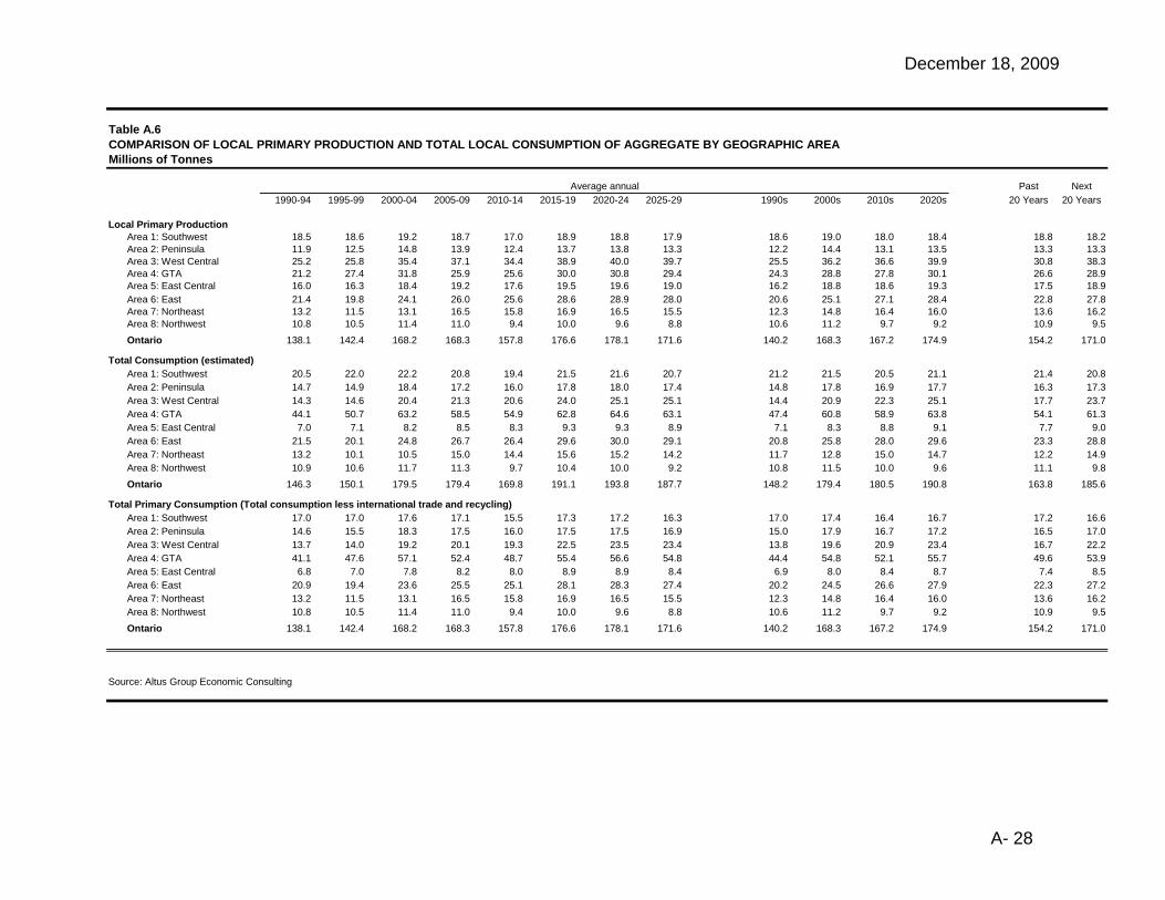
December 18, 2009

A- 28

Table A.6COMPARISON OF LOCAL PRIMARY PRODUCTION AND TOTAL LOCAL CONSUMPTION OF AGGREGATE BY GEOGRAPHIC AREAMillions of Tonnes

Past Next1990-94 1995-99 2000-04 2005-09 2010-14 2015-19 2020-24 2025-29 1990s 2000s 2010s 2020s 20 Years 20 Years

Local Primary ProductionArea 1: Southwest 18.5 18.6 19.2 18.7 17.0 18.9 18.8 17.9 18.6 19.0 18.0 18.4 18.8 18.2Area 2: Peninsula 11.9 12.5 14.8 13.9 12.4 13.7 13.8 13.3 12.2 14.4 13.1 13.5 13.3 13.3Area 3: West Central 25.2 25.8 35.4 37.1 34.4 38.9 40.0 39.7 25.5 36.2 36.6 39.9 30.8 38.3Area 4: GTA 21.2 27.4 31.8 25.9 25.6 30.0 30.8 29.4 24.3 28.8 27.8 30.1 26.6 28.9Area 5: East Central 16.0 16.3 18.4 19.2 17.6 19.5 19.6 19.0 16.2 18.8 18.6 19.3 17.5 18.9Area 6: East 21.4 19.8 24.1 26.0 25.6 28.6 28.9 28.0 20.6 25.1 27.1 28.4 22.8 27.8Area 7: Northeast 13.2 11.5 13.1 16.5 15.8 16.9 16.5 15.5 12.3 14.8 16.4 16.0 13.6 16.2Area 8: Northwest 10.8 10.5 11.4 11.0 9.4 10.0 9.6 8.8 10.6 11.2 9.7 9.2 10.9 9.5Ontario 138.1 142.4 168.2 168.3 157.8 176.6 178.1 171.6 140.2 168.3 167.2 174.9 154.2 171.0

Total Consumption (estimated)Area 1: Southwest 20.5 22.0 22.2 20.8 19.4 21.5 21.6 20.7 21.2 21.5 20.5 21.1 21.4 20.8Area 2: Peninsula 14.7 14.9 18.4 17.2 16.0 17.8 18.0 17.4 14.8 17.8 16.9 17.7 16.3 17.3Area 3: West Central 14.3 14.6 20.4 21.3 20.6 24.0 25.1 25.1 14.4 20.9 22.3 25.1 17.7 23.7Area 4: GTA 44.1 50.7 63.2 58.5 54.9 62.8 64.6 63.1 47.4 60.8 58.9 63.8 54.1 61.3Area 5: East Central 7.0 7.1 8.2 8.5 8.3 9.3 9.3 8.9 7.1 8.3 8.8 9.1 7.7 9.0Area 6: East 21.5 20.1 24.8 26.7 26.4 29.6 30.0 29.1 20.8 25.8 28.0 29.6 23.3 28.8Area 7: Northeast 13.2 10.1 10.5 15.0 14.4 15.6 15.2 14.2 11.7 12.8 15.0 14.7 12.2 14.9Area 8: Northwest 10.9 10.6 11.7 11.3 9.7 10.4 10.0 9.2 10.8 11.5 10.0 9.6 11.1 9.8Ontario 146.3 150.1 179.5 179.4 169.8 191.1 193.8 187.7 148.2 179.4 180.5 190.8 163.8 185.6

Total Primary Consumption (Total consumption less international trade and recycling)Area 1: Southwest 17.0 17.0 17.6 17.1 15.5 17.3 17.2 16.3 17.0 17.4 16.4 16.7 17.2 16.6Area 2: Peninsula 14.6 15.5 18.3 17.5 16.0 17.5 17.5 16.9 15.0 17.9 16.7 17.2 16.5 17.0Area 3: West Central 13.7 14.0 19.2 20.1 19.3 22.5 23.5 23.4 13.8 19.6 20.9 23.4 16.7 22.2Area 4: GTA 41.1 47.6 57.1 52.4 48.7 55.4 56.6 54.8 44.4 54.8 52.1 55.7 49.6 53.9Area 5: East Central 6.8 7.0 7.8 8.2 8.0 8.9 8.9 8.4 6.9 8.0 8.4 8.7 7.4 8.5Area 6: East 20.9 19.4 23.6 25.5 25.1 28.1 28.3 27.4 20.2 24.5 26.6 27.9 22.3 27.2Area 7: Northeast 13.2 11.5 13.1 16.5 15.8 16.9 16.5 15.5 12.3 14.8 16.4 16.0 13.6 16.2Area 8: Northwest 10.8 10.5 11.4 11.0 9.4 10.0 9.6 8.8 10.6 11.2 9.7 9.2 10.9 9.5Ontario 138.1 142.4 168.2 168.3 157.8 176.6 178.1 171.6 140.2 168.3 167.2 174.9 154.2 171.0

Source: Altus Group Economic Consulting

Average annual

December 18, 2009

A- 29

Table A.7POPULATION AND PER CAPITA PRODUCTION AND CONSUMPTION OF AGGREGATE BY GEOGRAPHIC AREA, ONTARIO


POPULATION (000s of Persons)Area 1: Southwest 1287.5 1334.6 1392.4 1429.8 1457.5 1503.8 1557.5 1613.2 1311.0 1411.1 1480.7 1585.3 1361.1 1533.0Area 2: Peninsula 1098.7 1134.7 1184.1 1216.5 1243.9 1291.0 1348.4 1411.1 1116.7 1200.3 1267.5 1379.8 1158.5 1323.6Area 3: West Central 1066.7 1161.0 1280.1 1379.5 1483.6 1610.3 1746.5 1878.3 1113.9 1329.8 1546.9 1812.4 1221.8 1679.7Area 4: GTA 4450.4 4865.2 5402.5 5905.7 6396.2 6822.6 7254.2 7646.4 4657.8 5654.1 6609.4 7450.3 5155.9 7029.8Area 5: East Central 483.5 499.9 518.8 537.5 551.9 572.5 594.2 612.7 491.7 528.2 562.2 603.5 509.9 582.8Area 6: East 1319.4 1383.0 1462.8 1517.4 1573.7 1644.5 1724.1 1805.4 1351.2 1490.1 1609.1 1764.7 1420.7 1686.9Area 7: Northeast 470.5 465.5 450.1 449.0 449.7 453.3 457.5 461.3 468.0 449.6 451.5 459.4 458.8 455.4Area 8: Northwest 385.0 382.5 369.9 363.5 355.8 353.8 352.9 351.7 383.7 366.7 354.8 352.3 375.2 353.5Ontario 10,561.7 11,226.3 12,060.8 12,798.9 13,512.5 14,251.7 15,035.2 15,780.1 10,894.0 12,429.9 13,882.1 15,407.6 11,661.9 14,644.9

SHARE OF POPULATION (%)Area 1: Southwest 12.2% 11.9% 11.5% 11.2% 10.8% 10.6% 10.4% 10.2% 12.0% 11.4% 10.7% 10.3% 11.7% 10.5%Area 2: Peninsula 10.4% 10.1% 9.8% 9.5% 9.2% 9.1% 9.0% 8.9% 10.3% 9.7% 9.1% 9.0% 9.9% 9.0%Area 3: West Central 10.1% 10.3% 10.6% 10.8% 11.0% 11.3% 11.6% 11.9% 10.2% 10.7% 11.1% 11.8% 10.5% 11.5%Area 4: GTA 42.1% 43.3% 44.8% 46.1% 47.3% 47.9% 48.2% 48.5% 42.8% 45.5% 47.6% 48.4% 44.2% 48.0%Area 5: East Central 4.6% 4.5% 4.3% 4.2% 4.1% 4.0% 4.0% 3.9% 4.5% 4.2% 4.0% 3.9% 4.4% 4.0%Area 6: East 12.5% 12.3% 12.1% 11.9% 11.6% 11.5% 11.5% 11.4% 12.4% 12.0% 11.6% 11.5% 12.2% 11.5%Area 7: Northeast 4.5% 4.1% 3.7% 3.5% 3.3% 3.2% 3.0% 2.9% 4.3% 3.6% 3.3% 3.0% 3.9% 3.1%Area 8: Northwest 3.6% 3.4% 3.1% 2.8% 2.6% 2.5% 2.3% 2.2% 3.5% 3.0% 2.6% 2.3% 3.2% 2.4%Ontario 100.0% 100.0% 100.0% 100.0% 100.0% 100.0% 100.0% 100.0% 100.0% 100.0% 100.0% 100.0% 100.0% 100.0%

POPULATION GROWTH (000s)Area 1: Southwest 13.1 8.8 12.5 4.5 7.4 10.0 11.1 11.1 10.9 8.5 8.7 11.1 9.7 9.9Area 2: Peninsula 8.9 8.4 10.2 4.1 7.4 10.4 12.0 12.8 8.6 7.2 8.9 12.4 7.9 10.7Area 3: West Central 21.7 20.5 24.4 17.5 23.5 26.5 26.9 26.4 21.1 20.9 25.0 26.7 21.0 25.8Area 4: GTA 66.2 92.2 111.6 101.0 89.9 86.9 82.6 78.3 79.2 106.3 88.4 80.5 92.7 84.4Area 5: East Central 7.7 2.6 4.9 2.3 3.7 4.3 4.1 3.6 5.1 3.6 4.0 3.8 4.4 3.9Area 6: East 22.0 9.5 17.0 10.0 12.1 15.1 16.3 16.1 15.8 13.5 13.6 16.2 14.6 14.9Area 7: Northeast 2.8 -3.0 -1.7 -0.1 0.5 0.8 0.9 0.7 -0.1 -0.9 0.7 0.8 -0.5 0.7Area 8: Northwest 0.8 -1.8 -1.7 -1.9 -0.9 -0.3 -0.2 -0.3 -0.5 -1.8 -0.6 -0.2 -1.1 -0.4Ontario 143.2 137.1 177.2 137.5 143.6 153.7 153.7 148.5 140.1 157.4 148.7 151.1 148.8 149.9

SHARE OF POPULATION GROWTH (%)Area 1: Southwest 9.1% 6.4% 7.1% 3.3% 5.2% 6.5% 7.2% 7.4% 7.8% 5.4% 5.9% 7.3% 6.5% 6.6%Area 2: Peninsula 6.2% 6.1% 5.8% 3.0% 5.2% 6.7% 7.8% 8.6% 6.2% 4.6% 6.0% 8.2% 5.3% 7.1%Area 3: West Central 15.2% 14.9% 13.8% 12.7% 16.4% 17.2% 17.5% 17.7% 15.1% 13.3% 16.8% 17.6% 14.1% 17.2%Area 4: GTA 46.2% 67.2% 63.0% 73.5% 62.6% 56.5% 53.7% 52.7% 56.5% 67.6% 59.4% 53.2% 62.3% 56.3%Area 5: East Central 5.4% 1.9% 2.7% 1.7% 2.6% 2.8% 2.7% 2.4% 3.6% 2.3% 2.7% 2.5% 2.9% 2.6%Area 6: East 15.4% 6.9% 9.6% 7.3% 8.4% 9.8% 10.6% 10.8% 11.2% 8.6% 9.1% 10.7% 9.8% 9.9%Area 7: Northeast 2.0% -2.2% -1.0% -0.1% 0.4% 0.5% 0.6% 0.4% 0.0% -0.6% 0.4% 0.5% -0.3% 0.5%Area 8: Northwest 0.5% -1.3% -0.9% -1.4% -0.6% -0.2% -0.1% -0.2% -0.4% -1.1% -0.4% -0.2% -0.8% -0.3%Ontario 100.0% 100.0% 100.0% 100.0% 100.0% 100.0% 100.0% 100.0% 100.0% 100.0% 100.0% 100.0% 100.0% 100.0%

Average annual

CONTINUED ON NEXT PAGE

December 18, 2009

A- 30

Table A.7 (continued)POPULATION AND PER CAPITA PRODUCTION AND CONSUMPTION OF AGGREGATE BY GEOGRAPHIC AREA, ONTARIO


POPULATION GROWTH RATE (%)Area 1: Southwest 1.0% 0.7% 0.9% 0.3% 0.5% 0.7% 0.7% 0.7% 0.8% 0.6% 0.6% 0.7% 0.7% 0.6%Area 2: Peninsula 0.8% 0.7% 0.9% 0.3% 0.6% 0.8% 0.9% 0.9% 0.8% 0.6% 0.7% 0.9% 0.7% 0.8%Area 3: West Central 2.1% 1.8% 1.9% 1.3% 1.6% 1.7% 1.6% 1.4% 1.9% 1.6% 1.6% 1.5% 1.8% 1.6%Area 4: GTA 1.5% 1.9% 2.1% 1.7% 1.4% 1.3% 1.2% 1.0% 1.7% 1.9% 1.4% 1.1% 1.8% 1.2%Area 5: East Central 1.6% 0.5% 0.9% 0.4% 0.7% 0.8% 0.7% 0.6% 1.1% 0.7% 0.7% 0.6% 0.9% 0.7%Area 6: East 1.7% 0.7% 1.2% 0.7% 0.8% 0.9% 1.0% 0.9% 1.2% 0.9% 0.8% 0.9% 1.1% 0.9%Area 7: Northeast 0.6% -0.6% -0.4% 0.0% 0.1% 0.2% 0.2% 0.1% 0.0% -0.2% 0.1% 0.2% -0.1% 0.2%Area 8: Northwest 0.2% -0.5% -0.4% -0.5% -0.3% -0.1% 0.0% -0.1% -0.1% -0.5% -0.2% -0.1% -0.3% -0.1%Ontario 1.4% 1.2% 1.5% 1.1% 1.1% 1.1% 1.0% 1.0% 1.3% 1.3% 1.1% 1.0% 1.3% 1.0%

PER CAPITA PRODUCTION OF AGGREGATES (Tonnes)Area 1: Southwest 14.4 13.9 13.8 13.1 11.7 12.6 12.1 11.1 14.2 13.4 12.1 11.6 13.8 11.9Area 2: Peninsula 10.8 11.0 12.5 11.4 10.0 10.6 10.2 9.4 10.9 12.0 10.3 9.8 11.5 10.1Area 3: West Central 23.7 22.1 27.6 26.9 23.1 24.1 22.9 21.2 22.9 27.2 23.6 22.1 25.1 22.8Area 4: GTA 4.8 5.6 5.9 4.4 4.0 4.4 4.3 3.8 5.2 5.1 4.2 4.0 5.2 4.1Area 5: East Central 33.1 32.6 35.4 35.7 32.0 34.0 33.0 31.1 32.9 35.6 33.0 32.0 34.2 32.5Area 6: East 16.2 14.3 16.5 17.2 16.3 17.4 16.8 15.5 15.3 16.8 16.8 16.1 16.0 16.5Area 7: Northeast 28.0 24.7 29.1 36.8 35.1 37.3 36.1 33.6 26.4 33.0 36.2 34.8 29.7 35.5Area 8: Northwest 28.0 27.4 30.9 30.2 26.5 28.3 27.3 25.2 27.7 30.5 27.4 26.2 29.1 26.8Ontario 13.1 12.7 14.0 13.2 11.7 12.4 11.9 10.9 12.9 13.6 12.0 11.4 13.2 11.7

PER CAPITA CONSUMPTION OF AGGREGATES (Tonnes)Area 1: Southwest 16.0 16.5 16.0 14.5 13.3 14.3 13.8 12.8 16.2 15.3 13.8 13.3 15.7 13.6Area 2: Peninsula 13.4 13.1 15.5 14.2 12.8 13.8 13.3 12.3 13.2 14.9 13.3 12.8 14.0 13.1Area 3: West Central 13.4 12.6 16.0 15.5 13.9 14.9 14.4 13.3 13.0 15.7 14.4 13.9 14.4 14.1Area 4: GTA 9.9 10.4 11.7 9.9 8.6 9.2 8.9 8.2 10.2 10.8 8.9 8.6 10.5 8.7Area 5: East Central 14.5 14.2 15.7 15.8 15.1 16.2 15.7 14.5 14.4 15.8 15.6 15.1 15.1 15.4Area 6: East 16.3 14.5 17.0 17.6 16.8 18.0 17.4 16.1 15.4 17.3 17.4 16.8 16.4 17.1Area 7: Northeast 28.0 21.8 23.3 33.4 32.1 34.4 33.3 30.9 24.9 28.4 33.3 32.1 26.6 32.7Area 8: Northwest 28.4 27.7 31.7 31.0 27.3 29.3 28.3 26.3 28.1 31.3 28.3 27.3 29.7 27.8Ontario 13.9 13.4 14.9 14.0 12.6 13.4 12.9 11.9 13.6 14.5 13.0 12.4 14.0 12.7

Source: Altus Group Economic Consulting based on data from TOARC, StatCan and Ministry of Finance

Average annual

December 18, 2009

A- 31

Table A.8

REGRESSION MODEL TO PROJECT PER CAPITA AGGREGATE CONSUMPTION

TimeTotal

population

Total population

GrowthHousing

startsReal GDP

growth UR

Total aggregate consumption (tonnes, millions)

Per capita aggregate consumption (tonnes)

Model Fitted per capita values (tonnes)

000s 000s 000s % %1980 10 8746.0 83.9 40.1 3.3 6.9 123.2 14.1 14.2 Linear Multiple Regression

1981 11 8812.3 66.3 50.2 4.8 6.6 124.1 14.1 14.71982 12 8920.3 108.0 38.5 -2.7 9.8 108.3 12.1 13.2 Key Regression Statistics1983 13 9039.6 119.3 54.9 4.5 10.4 116.7 12.9 14.1

1984 14 9167.5 127.9 48.2 7.9 9.0 132.5 14.5 14.3 Regression Statistics1985 15 9294.7 127.2 64.9 4.2 8.0 152.5 16.4 15.7 Multiple R 0.951986 16 9437.4 142.7 81.5 4.1 7.0 173.5 18.4 17.3 R Square 0.911987 17 9637.9 200.6 105.2 5.0 6.1 194.4 20.2 20.1 Adjusted R Square 0.891988 18 9838.6 200.7 99.9 5.4 5.0 206.6 21.0 20.0 Standard Error 0.791989 19 10103.3 264.7 93.3 3.4 5.0 208.3 20.6 20.3 Observations 291990 20 10295.8 192.5 62.6 -1.7 6.2 170.1 16.5 16.51991 21 10431.3 135.5 52.8 -3.9 9.5 143.0 13.7 13.4 ANOVA1992 22 10572.2 140.9 55.8 0.9 10.8 135.6 12.8 13.1 df SS MS F Significance 1993 23 10690.0 117.8 45.1 1.0 10.9 138.8 13.0 11.8 Regression 5 141.2925453 28.25851 44.77819 4.1891E-111994 24 10819.1 129.1 46.6 5.9 9.6 143.9 13.3 12.5 Residual 23 14.51478438 0.6310781995 25 10950.1 131.0 35.8 3.5 8.7 137.9 12.6 12.1 Total 28 155.80732961996 26 11082.9 132.8 43.1 1.1 9.0 144.4 13.0 12.41997 27 11227.7 144.7 54.1 4.5 8.4 151.6 13.5 13.4 Coefficients Standard Error t Stat1998 28 11365.9 138.3 53.8 4.8 7.2 152.6 13.4 13.7 Intercept 20.660 2.156 9.61999 29 11504.8 138.9 67.2 7.5 6.3 164.2 14.3 14.8 Total population -0.001 0.000 -7.12000 30 11683.3 178.5 71.5 5.9 5.8 183.5 15.7 15.8 Population growth 0.016 0.005 3.12001 31 11896.7 213.4 73.3 1.8 6.3 179.9 15.1 16.0 Unemployment rate -0.407 0.129 -3.12002 32 12091.0 194.4 83.6 3.1 7.1 175.6 14.5 15.9 Housing starts 0.066 0.014 4.82003 33 12242.3 151.2 85.2 1.4 6.9 175.0 14.3 15.2 Real GDP % 0.026 0.057 0.42004 34 12390.6 148.3 85.1 2.6 6.8 183.4 14.8 15.12005 35 12528.5 137.9 78.8 2.8 6.6 184.5 14.7 14.52006 36 12665.3 136.9 73.4 2.6 6.3 189.3 14.9 14.12007 37 12793.6 128.2 68.1 2.3 6.4 184.6 14.4 13.52008 38 12929.0 135.4 75.1 -0.4 6.5 178.4 13.8 13.9

Source: Altus Group Economic Consulting based on data from Ministry of Natural Resources and TOARC

December 18, 2009

A- 32

Table A.9Summary of Key Information Sources for Projection Exercise

Series Source Document/Database

Historical annual aggregate production data Pre 1985Mineral Score

1985-1998 Ontario Ministry of Natural Resources Statistical Update1998 On TOARC Mineral Aggregates in Ontario: Statistical Update

Recycling estimates LVM-Jegel SAROS Paper 4: Recyling and Reuse

International trade in aggregate products Statistics Canada CANSIM (see separate listing of individual cansim numbers)

Internal aggregate trade (between subareas) Altus Group Economic Consulting Estimates based on:Previous researchAnalysis of construction spending patternsAnalysis of per capita production patterns in each subarea to determine likely "excesses"Discussions with knowledgeable sources on likely movements

Historical annual total population Ontario and 8 subareas Statistics Canada Annual demographic statistics (electronic data files)8 subareas amalgamated from individual Census Divisions (CDs)

Projected total population GGH census divisions (CDs): Ontario Ministry of PIR Places to Growth: Growth Plan for the Greater Goldern Horseshoe, 2006Other CDs: Ontario Ministry of Finance Ontario Population Projections, 2008-2036, 2009 updateOntario total: Sum of GGH and remaining areas8 subareas: Amalgamated from component CDs

Historical real GDP Statistics Canada Provincial Economic AccountsHistorical unemployment rate Statistics Canada Labour Force Survey

Projected real GDP growth 2009-2012 Ontario Ministry of Finance Ontario Economic Outlook and Fiscal Review 2009Projected unemployment rate 2026-2029 Altus Group Economic Consulting Extrapolated trend

Historical housing starts CMHC Electronic data files

Projected housing starts Ontario MOF 2009-2011 Ontario Economic Outlook and Fiscal Review 20092012-2025 Toward 2025: Assessing Ontario's Long-Term Outlook2026-2029 extrapolated trend based on population growth patterns

Historical construction spending by type New residential Statistics Canada Provincial Economic AccountsNew total non-res building Statistics Canada Provincial Economic Accounts% of total new non- Pre 1993 Statistics Canada Construction in Canada res building by type 1993 on Statistics Canada CANSIM table 026-0016Repair Pre 1993 Statistics Canada Construction in Canada

1993 on Statistics Canada CANSIM table 032-0032

Ontario Ministry of Northern Development, Mines & Forestry

December 18, 2009

A- 33

Table A.10INTERNATIONAL TRADE AGGREGATE RELATED HS CODES

25210000 Limestone flux, limestone & other calcareous stone for lime or cement 2521000010 2521000010 Limestone flux 2521000020 2521000020 Agricultural limestone for soil improvement 2521000030 2521000030 Limestone nes 2521000090 2521000090 Limestone flux 25183 Dolomite ramming mix 25183 Dolomite ramming mix 25182 Calcined or sintered dolomite 25182 Dolomite calcined or sintered 25181 Dolomite not calcined or sintered 25181 Dolomite not calcined or sintered 25174900 Granules chippings & powder nes of 25.15 or 25.16 heat-treated or not 251749002517490010 2517490010 Limestone granuleschippings and powder roofing granules heat treated or not 2517490090 2517490090 Granuleschippings & powder of stones of 25.15 or 25.16nes w/n heat-treated 25174920 Roofing granules 251749202517499 Granules chippings & powder nes of 25.15 or 25.16 heat-treated or not 2517499 Granuleschippings & powder of stones of 25.15 or 25.16nes w/n heat-treated 2517491 Limestone granules chippings & powder (excluding roofing granules) 2517491 Limestone granuleschippings and powder roofing granules heat treated or not 251741 Marble granules chipping & powder of 25.15 or 25.16 heat-treated or not 251741 Marble granules chippings and powder whether or not heat-treated 25173 Tarred macadam 25173 Tarred macadam 25172 Macadam of slag dross or similar industrial waste etc 25172 Macadam of slag dross or similar industrial waste etc 2517109 Stone broken or crushed nes used for aggregates etc 25171092517102 Limestone except pebbles and gravel used for aggregates etc 251710225171010 Pebbles and gravel used for aggregates etc 251710102517100010 2517100010 Pebbles or gravel used for concrete aggregates etc 2517100020 2517100020 Flint 2517100030 2517100030 Limestone other than hd 25.21 used for concrete aggregates etc 2517100090 2517100090 Broken or crushed stone nes used for concrete aggregates etc 2516121000 2516121000 Granite merely cut by sawing into blocks or slabs of a rectangular shape 2516129000 2516129000 Granitemerely cut o/t by sawing into blocks or slabs of a rectangular shape 25169000 Monumental or building stone nes 251690002516901000 2516901000 Monumental or building stone nes crude or roughly trimmed 2516901010 2516901010 Limestone monumental or building crude or roughly trimmed 2516901090 2516901090 Monumental or building stone o/t limestone crude or roughly trimmed nes 2516902000 2516902000 Monum or bldg stonenes merely cut into blocks or slabs of a rectangular shape 2516902010 2516902010 Limestone merely cut into slabs or blocks rectangular shape 2516902090 2516902090 Monum or bldg stonenes merely cut into blocks or slabs of a rectangular shape 251622 Sandstone merely cut by sawing or otherwise into blocks etc 251622 Sandstone merely cut by sawing or o/winto blocks/slabs of a rectangular shape 251621 Sandstone crude or roughly trimmed 251621 Sandstone crude or roughly trimmed 251612 Granite merely cut by sawing or otherwise into blocks etc 251612 Granitemerely cut by sawing into blocks or slabs of a rectangular shape 251611 Granite crude or roughly trimmed 251611 Granite crude or roughly trimmed 25140000 Slate whether or not roughly trimmed or merely cut etc 251400002514001000 2514001000 Slate crude or roughly trimmed 2514002000 2514002000 Slate merely cut by sawing or otherwise into blocks/slabs rectangular shape 2514009000 2514009000 Slate nes including powder and waste 2514009010 2514009010 Slate crude or roughly trimmed 2514009090 Slate nes including powder and waste 2514009090 Slate nes including powder and waste 251319 Pumice stone nes 251319 Pumice stone nes 251311 Pumice stones, crude or in irregular pieces incl crushed (bimskies) 251311 Pumice stone crude or in irregular pieces incl crushed pumiste(bimskies) 25059 Natural sands nes exc metal bearing sands of Chapter 26 25059 Natural sands nes exc metal bearing sands of Chapter 26 2505900010 2505900010 Olivine sand 2505900090 2505900090 Natural sands nes exc metal bearing sands of Chapter 26

Export Import

SAROS Paper 1 - Aggregate Consumption and Demand

Appendix BAggregate Factors for Specific Construction Applications -Background Calculations

LVM-JegelNovember 2009

2 Lane Highway(Source: Typical Municipal Highway - Client)

Shoulder (m) Lane (m) Lane (m) Shoulder (m)2 3.75 3.75 2

LENGTH (m)1000

THICKNESS (m)Hot Mix Asphalt 0.1Granular A 0.2Granular B 0.45

Assumption: 95% of asphalt layer is aggregate

2 Shoulders 4 m2 Lanes 7.5 m

Total Amount of Aggregate in Asphalt (95%) 1093 m3 2485 TonnesTotal Amount of Granular A Required 2300 m3 5003 TonnesTotal Amount of Granular B Required 5175 m3 10738 TonnesTotal Amount of Aggregate Required 8568 m3 18226 Tonnes

WIDTH OF HIGHWAY

4 Lane Highway(Source: Typical Municipal Highway - Client)

Shoulder (m) Lane (m) Lane (m) Lane (m) Lane (m) Shoulder (m)2 3.75 3.75 3.75 3.75 2

LENGTH (m)1000

THICKNESS (m)Hot Mix Asphalt 0.1Granular A 0.2Granular B 0.45

Assumption: 95% of asphalt layer is aggregate

2 Shoulders 4 m4 Lanes 15 m

Total Amount of Aggregate in Asphalt (95%) 1805 m3 4106 TonnesTotal Amount of Granular A Required 3800 m3 8265 TonnesTotal Amount of Granular B Required 8550 m3 17741 TonnesTotal Amount of Aggregate Required 14155 m3 30113 Tonnes

WIDTH OF HIGHWAY

185 Square Meter House(Source: Typical Housing Plan - Ranch Style)

DimensionsLength 18.3 mWidth 9.1 m

Perimeter 55 m

Height of Foundation Wall 3.5 mThickness 0.15 m

Volume of Foundation Wall 29 m3

Slab on GradeArea 167 m2Thickness 0.125 m

Volume of Slab on Grade 21 m3Total Volume of Concrete = Vol. SOG + Vol. Foundation Walls 50 m3

Thickness of Granular Material under Slab on Grade 0.1 mVolume of Granular Material under Slab 17 m3

Driveway DimensionsLength 9 mWidth 6 m

Thickness of Granular Base 0.15 mThickness of Asphalt 0.05 m(Assumption: 95% aggregates in asphalt mix)Volume of Granular Base 8.2 m3Volume of Asphalt Aggregates 2.6 m3

Perimeter Drainage Perimeter 55 mHeight 2 mThickness 0.2 mVolume of Granular Material for Drainage 22 m3

Brick Surface AreaPerimeter 55 mHeight 3 mMinus area of windows, doors and garage 38 m2Net Brick Surface Area 129 m2Thickness 0.1 mTotal Volume of Bricks 13 m3

Concrete SidewalkWidth 1.5 m

Length 22.3 mArea 33 m2Thickness 0.125 mVolume 4.2 m3

HardscapingWalkway in Front of House (Concrete Pavers)Width 1.5 mLength 9 mThickness 0.06 mVolume 0.8 m3

Walkway at Side of House (Concrete Pavers)Width 0.75 mLength 11 mThickness 0.06 mVolume 0.5 m3

ShinglesArea of RoofSlopes Surfaces (based on 18.4 degree roof slope) 9.6 mLength 18 mSurface area of shingles 176 m2

Mineral Granules Pressed onto Shingles (Crushed Granite)Thickness 0.001 mArea 176 m2Volume 0.18 m3

Trenches for Water and Sewer ServicesWidth 0.3 mDepth 0.3 mSubtract Area of 12mm pipe 0.00011 m2Length 9 mVolume of Aggregates in Trench 1 m3

Total Amount of Brick (including mortar) 13 m3 20 TonnesTotal Amount of Aggregate in Shingles 0.18 m3 0.4 TonnesTotal Amount of Granular Material Required (base, drainage, trench) 48 m3 99 TonnesTotal Amount of Aggregates in Asphalt 2.6 m3 6 TonnesTotal Amount of Concrete Aggregate Required 55 m3 133 TonnesTotal Amount of Aggregate Required 118 m3 257 Tonnes

Wind Turbine(Source: Previous LVM-JEGEL Experience)

Foundation (Type 2)

Area of Base of Foundation

Dimensions of Square 18 m x 18 m 324 m2Subtract to get Octagon 56 m2

Area of Octagonal Base 268 m2

Height 1.7 m

Volume of Concrete Foundation 456 m3Plus top 27 m3

Total Volume of Concrete 483 m3

Aggregates for Drainage

Rock DrainArea 20 m2Height 3.5 m

Volume of Rock Drain 69 m3

Access Road (Gravel Surface)

Length 500 mWidth 6.0 mThickness of Granular A 0.15 mThickness of Granular B 0.25 m

Total Amount of Aggregate in Concrete Mix 483 m3 1160 TonnesTotal Amount of Granular A 450 m3 979 TonnesTotal Amount of Granular B (Drainage Aggregates & Road) 819 m3 1699 TonnesTotal Amount of Aggregate Required 1752 m3 3838 Tonnes

4 Lane Concrete Bridge over 6 Lane Highway (83 meters long)(Source: Typical Provincial Overpass - Client)

Concrete VolumesSub-Structure 788 m3Super-Structure 1439 m318 NU Girders 613 m3

Total Volume of Concrete for Bridge Structure 2840 m3

80 mm asphalt over deck: 0.08 mlength of deck 83.5 mwidth of deck 23.3 m

50 mm asphalt over approaches: 0.1 mlength of approaches 48.1 mwidth of approaches 23.3 m

Volume of asphalt on deck and approaches 211.6 m3Volume of aggregates based on 95% 201.1 m3

Total Amount of Aggregate Required 3041 m3 7299 Tonnes

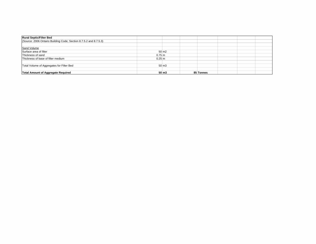
Rural Septic/Filter Bed(Source: 2006 Ontario Building Code; Section 8.7.5.2 and 8.7.5.3)

Sand VolumeSurface area of filter 50 m2Thickness of sand 0.75 mThickness of base of filter medium 0.25 m

Total Volume of Aggregates for Filter Bed 50 m3

Total Amount of Aggregate Required 50 m3 85 Tonnes

1000 m2 of Office Space, Hospital or School(Source: Previous Dessau/LVM-Technisol Experience)

Concrete Slab on Grade150 mm Slab, 32m long x 32 m wide = 154 m3 of concreteAdd 10% spillage and uneven surface = 170 m3 of concrete

Quantity of Coarse Aggregate 71.3 m3Quantity of Fine Aggregate 45 m3Total Quantity of Aggregate required in concrete mix 116.3 m3

Quantity of Sub-base under the slabArea of subbase (3.05 m additional to perimeter of slab) 1230 m2Volume of 100 mm thick sub-base of well graded rock or gravel (coarse aggregate) 145 m3Volume of 50 mm thick coarse sand (fine aggregate) 72.5 m3Total Volume of Sub-base Aggregate 217.5 m3

Total Amount of Aggregate in Concrete Mix 116.3 m3 279 TonnesTotal Amount of Sub-Base Aggregate 217.5 m3 451 TonnesTotal Volume of Aggregate Required 334 m3 730 Tonnes

1 km of Railway Bed(Source: Previous LVM-JEGEL Experience)

Railway Ballast 1.14 m2Areas 0.19 m2

0.95 m2

Multiplied by 2 2.28 m2Total Railway Ballast 2.28 m2

top (Concrete) 0.64 m2

Railway Ballast Plus Concrete Aggregates 2.28 m2

Multiplied by 1 km 2276.3 m3

Total Amount of Railway Ballast Required 2276.3 m3 4553 TonnesTotal Amount of Concrete Aggregates Required 638.7 m3 1533 TonnesTotal Amount of Aggregates Required 2276 m3 6086 Tonnes

1 km Underground Sewer Line - Under a Boulevard(Source: City of Toronto Standard Cross-Sections)

MANHOLE - one every 100 mWall thickness 0.133 mheight 4.5 mPerimeter 4.6 mOuter Wall Diameter 1.5 m Area 1.7 m2Inner Wall Diameter 1.2 m Area 1.1 m2

Total Volume 3 m3

FLAT CAP TOP (& Bottom)

thicnkess 0.22 marea 2 m2Total Volume 0.37 m3

x2 (To include bottom) 0.75 m3

BASElength 2.07 mdepth 0.18 mTotal Volume 0.8 m3

Total Volume of Aggregates in Concrete for 10 Manholes 40.2 m3

600 mm SEWER

Concrete Bedding Sewer Pipe Diameter 0.6 mTrench Width 0.9 m150 mm min on each side of pipe

height 0.45 mlength 1000 m

Volume of Concrete Below Pipe 405 m3

MINUS half pipe diameterarea 0.14 m2volume 141.4 m3

Net volume of aggregates in concrete bedding 263.6 m3Volume of aggregates in concrete sewer pipe 86.4 m3(based on 100mm thick walls)

Total Amount of Backfill Material 674.6 m3 1450 TonnesTotal Amount of Concrete Aggregates Required 390 m3 936 TonnesTotal Amount of Aggregates Required 1065 m3 2387 Tonnes

1 km Underground Sewer Line - Under a Road(Source: City of Toronto Standard Cross-Sections)

MANHOLE - one every 100 mWall thickness 0.133 mheight 4.5 mPerimeter 4.6 mOuter Wall Diameter 1.5 m Area 1.7 m2Inner Wall Diameter 1.2 m Area 1.1 m2

Total Volume 3 m3

FLAT CAP TOP (& Bottom)

thicnkess 0.22 marea 2 m2Total Volume 0.37 m3

x2 (To include bottom) 0.75 m3

BASElength 2.07 mdepth 0.18 mTotal Volume 0.8 m3

Total Volume of Aggregates in Concrete for 10 Manholes 40.2 m3

600 mm SEWER

Concrete Bedding Sewer Pipe Diameter 0.6 m

0.9 m150 mm min on each side of pipe

height 0.45 mlength 1000 m

Volume of Concrete Below Pipe 405 m3

MINUS half pipe diameterarea 0.14 m2volume 141.4 m3

Volume of aggregates in concrete sewer pipe 86.4 m3(based on 100mm thick walls)Volume of aggregates in concrete bedding 263.6 m3

REINSTATE ROAD

Length 1000 mWidth of Trench 1.4 m

Layers: From Road Surface

HL-1 0.04 mHL-8 0.14 mGranular A 0.15 mGranular B 0.15 mU-Fill 3.47 mBackfill Material 0.6 mConcrete Bedding 0.45 m

Volume of Aggregates in Asphalt (based on 95%) 232.6 m3 529 TonnesVolume of Granular A 204.0 m3 444 TonnesVolume of Granular B 204.0 m3 423 TonnesVolume of U-Fill 4719.2 m3 10618 TonnesVolume of Backfill Material 674.6 m3 1450 TonnesVolume of Aggregates (Concrete Pipe, Manholes & Bedding) 390.2 m3 936 Tonnes

Total Amount of Aggregates Required 6425 m3 14401 Tonnes

1 km Underground Water Pipe - Under a Boulevard (Southern Ontario)(300 mm Diameter)(Source: City of Toronto Standard Cross-Sections)

Typical Depth of Watermain 2 mDiameter of Pipe 0.3 mLength 1000 m

BeddingDepth of Granular A 0.3 mDepth of Granular B 0.45 m

Width 0.7 m

Net Area of Granular A 0.17 m2Net Area of Granular B 0.28 m2

Total Volume of Granular A 175 m3 380 TonnesTotal Volume of Granular B 280 m3 580 Tonnes

Total Volume of Aggregates 454 m3 960 Tonnes

1 km Underground Water Pipe - Under a Road (Southern Ontario)(300 mm Diameter)(Source: City of Toronto Standard Cross-Sections)



Width 0.7 m


Volume of Granular A (Bedding) 175 m3Volume of Granular B (Bedding) 280 m3

REINSTATE ROAD



HL-1 0.04 mHL-8 0.14 mGranular A 0.15 mGranular B 0.15 mU-Fill 0.77 m

Volume of Aggregates in Asphalt (based on 95%) 119.7 m3 272 TonnesTotal Volume of Granular A (Bedding & Base) 279.7 m3 608 TonnesTotal Volume of Granular B (Bedding & Subbase) 384.7 m3 798 TonnesVolume of U-Fill 539 m3 1213 Tonnes


*Northern Ontario Calculations: Based on 2.2m frost depth1 km Underground Water Pipe - Under a Boulevard (Northern Ontario)(300 mm Diameter)(Source: City of Toronto Standard Cross-Sections - Modified to Northern Ontario Conditions for Larger Frost Depth)



Width 0.7 m


Total Volume of Granular A 175 m3 380 TonnesTotal Volume of Granular B 280 m3 580 Tonnes


1 km Underground Water Pipe - Under a Road (Northern Ontario)(300 mm Diameter)(Source: City of Toronto Standard Cross-Sections - Modified to Northern Ontario Conditions for Larger Frost Depth)



Width 0.7 m


Volume of Granular A (Bedding) 175 m3Volume of Granular B (Bedding) 280 m3

REINSTATE ROAD



HL-1 0.04 mHL-8 0.14 mGranular A 0.15 mGranular B 0.15 mU-Fill 1.77 m

Volume of Aggregates in Asphalt (based on 95%) 119.7 m3 272 TonnesTotal Volume of Granular A (Bedding & Base) 279.7 m3 608 TonnesTotal Volume of Granular B (Bedding & Subbase) 384.7 m3 798 TonnesVolume of U-Fill 1239 m3 2788 Tonnes


*Assumption for Roads: Urban Cross-Sections: No Shoulders on these roads

1 km of Major Arterial Road (Southern Ontario)(Source: City of Toronto Standard Cross-Sections)

AADT=50,000Truck Routes (10% Commercial Vehicles)30 Mpa Subgrade

HL-1 40 mm 0.04 mHL-8 (HS) 150 mm 0.15 mGranular A 150 mm 0.15 mGranular B 250 mm 0.25 mTOTAL 590 mm 0.59 m

Assuming 95% Aggregates in AsphaltLane Width 3.75 mPER LANE KM 2177 m3Number of lanes 4

Total Volume of HL-1 for 4 Lanes 570 m3 1297 TonnesTotal Volume of HL-8 2137.5 m3 4863 TonnesTotal Volume of Granular A 2137.5 m3 4649 TonnesTotal Volume of Granular B 3562.5 m3 7392 Tonnes


1 km of Minor Arterial Road (Southern Ontario)(Source: City of Toronto Standard Cross-Sections)

AADT=25,000Truck Routes (7.5% Commercial Vehicles)30 Mpa Subgrade



Total Volume of HL-1 for 4 Lanes 285.0 m3 648 TonnesTotal Volume of HL-8 997.5 m3 2269 TonnesTotal Volume of Granular A 1068.8 m3 2325 TonnesTotal Volume of Granular B 1068.8 m3 2218 Tonnes


1 km of Collector (Southern Ontario)(Source: City of Toronto Standard Cross-Sections)

AADT=10,000Comm./Ind. (5% Commercial Vehicles)30 Mpa Subgrade

HL-3 40 mm 0.04 mHL-8 115 mm 0.115 mGranular A 150 mm 0.15 mGranular B 150 mm 0.15 mTOTAL 455 mm 0.455 m




1 km of Local Road (Southern Ontario)(Source: City of Toronto Standard Cross-Sections)

AADT=3,000Local Industrial (10% Commercial Vehicles)30 Mpa Subgrade



Total Volume of HL-1 for 4 Lanes 285 m3 648 TonnesTotal Volume of HL-8 570 m3 1297 TonnesTotal Volume of Granular A 1068.75 m3 2325 TonnesTotal Volume of Granular B 1068.75 m3 2218 Tonnes


1 km of Major Arterial Road (Northern Ontario)(Source: Ontario Ministry of Transportation Pavement Design and Rehabilitation Manual)

AADT=50,000Truck Routes (10% Commercial Vehicles)30 Mpa Subgrade





1 km of Minor Arterial Road (Northern Ontario)(Source: Ontario Ministry of Transportation Pavement Design and Rehabilitation Manual)

AADT=25,000Truck Routes (7.5% Commercial Vehicles)30 Mpa Subgrade





1 km of Collector (Northern Ontario)(Source: Ontario Ministry of Transportation Pavement Design and Rehabilitation Manual)

AADT=10,000Comm./Ind. (5% Commercial Vehicles)30 Mpa Subgrade





1 km of Local Road (Northern Ontario)(Source: Ontario Ministry of Transportation Pavement Design and Rehabilitation Manual)

AADT=3,000Local Industrial (10% Commercial Vehicles)30 Mpa Subgrade

HL-3 50 mm 0.05 mHL-8 0 mm 0 mGranular A 150 mm 0.15 mGranular B 600 mm 0.6 mTOTAL 800 mm 0.8 m


Total Volume of HL-1 for 2 Lanes 356.25 m3 810 TonnesTotal Volume of HL-8 0 m3 0 TonnesTotal Volume of Granular A 1068.75 m3 2325 TonnesTotal Volume of Granular B 4275 m3 8871 Tonnes


1 km of 4-Lane Freeway(Source: Typical Provincial Freeway - Client)

Shoulder (m) Lane (m) Lane (m) Shoulder (m) Shoulder (m) Lane (m) Lane (m) Shoulder (m)3 3.7 3.7 3.7 3.7 3.7 3.7 3

LENGTH (m)1000

DEPTH (m)Hot Mix Asphalt Aggregates (95% of HMA thickness) 0.228Granular A 0.15Granular B 0.35

Assumption: Asphalt layer consists of 95% aggregate

4 Shoulders - Asphalt Aggregate 3055.2 m34 Lanes - Asphalt Aggregate 3374.4 m34 Shoulders - Granular A 2010.0 m34 Lanes - Granular A 2220.0 m34 Shoulders - Granular B 4690.0 m34 Lanes - Granular B 5180.0 m3

Total Amount of Asphalt Aggregate 6430 m3 14627 TonnesTotal Amount of Granular A 4230 m3 9200 TonnesTotal Amount of Granular B 9870 m3 20480 Tonnes

Total Amount of Aggregates 20530 m3 44308 Tonnes

WIDTH OF FREEWAY

Laneway (1 km)(Source: City of Vaughan Engineering Standard - Local and Rural Residential Road Standards)

Length 1000 mWidth of Pavement 6 mConcrete Pad (1m on each side) 2 mThickness of Concrete 0.175 m

Pavement StructureHL-3 0.04 mHL-8 0.05 mBase:20mm crusher-run limestone 0.15 m50mm crusher-run limestone 0.2 m

Total Amount of Concrete Aggregate 350 m3 840 TonnesTotal Amount of HL-3 240 m3 546 TonnesTotal Amount of HL-8 300 m3 683 TonnesTotal Amount of 20mm crusher-run limestone 900 m3 1935 TonnesTotal Amount of 50mm crusher run-limestone 1200 m3 2640 Tonnes

Total Amount of Aggregates 2990 m3 6644 Tonnes

Parking(Source: Previous LVM-JEGEL Experience)

Typical Parking SpaceLength 5 mWidth 2.75 m

Pavement Structures

Underground Parking Garage Slab on GradeThickness of Concrete 0.15 mThickness of Granular 0.15 m

Suspended SlabThickness of Concrete 0.2 m

At-Grade Parking Lot (Outdoor)Thickness of Concrete 0.2 mThickness of Granular A 0.15 mThickness of Granular B 0.15 m

Aggregate Quantities

Underground Parking Garage Slab on GradeTotal Amount of Concrete Aggregate 2.1 m3 5 TonnesTotal Amount of Granular B 2.1 m3 4 TonnesTotal Amount of Aggregates 4.1 m3 9 Tonnes

Suspended SlabTotal Amount of Concrete Aggregate 2.8 m3 7 TonnesTotal Amount of Aggregates 2.8 m3 7 Tonnes

At-Grade Parking Lot (Outdoor)Total Amount of Concrete Aggregate 2.8 m3 7 TonnesTotal Amount of Granular A 2.1 m3 4 TonnesTotal Amount of Granular B 2.1 m3 4 TonnesTotal Amount of Aggregates 7 m3 15 Tonnes

SAROS Paper 1 - Aggregate Consumption and Demand Appendix C Analysis of Impact of Development Trends on Aggregate Consumption MHBC Planning October 2009

December 18, 2009

MHBC Planning Page 2

TABLE OF CONTENTS

Page

1.0 Introduction .............................................................................4

2.0 Current Aggregate Usage Patterns .......................................6

3.0 Population & Employment Growth Projections ...................7 3.1 Growth Plan for the Greater Golden Horseshoe ............................................8

4.0 Influencing Trends in Urban Form.......................................11 4.1 Urban Structure ............................................................................................11

4.1.1 Neighbourhood Street Patterns .......................................................12 4.1.2 Growth Boundaries and Suburban Development............................13 4.1.3 Intensification and Infilling ...............................................................14 4.1.4 Reuse and Redevelopment .............................................................15 4.1.5 Mixed Use Development .................................................................16

4.2 Built Form .....................................................................................................17 4.2.1 Demographics and Demand Shift....................................................17 4.2.2 Height and Density Standards.........................................................19 4.2.3 Urban Design Trends.......................................................................20 4.2.4 Sustainable Development Practices................................................20

4.3 Mobility..........................................................................................................21 4.3.1 Investment in Public Transit ............................................................22 4.3.2 Major Transportation Infrastructure Initiatives .................................24 4.3.3 Travel Demand ................................................................................26

5.0 Impact of Trends on Aggregate Consumption Patterns....29 5.1 Street Patterns and Standards .....................................................................29

5.1.1 Street Pattern (grid vs. curvilinear patterns)....................................29 5.1.2 Road Design Standards ..................................................................33 5.1.3 The Provision of Parking .................................................................35 5.1.4 Major Infrastructure..........................................................................36

5.2 Built Form .....................................................................................................38 5.2.1 Distribution and Size of Housing Types ..........................................39

5.3 Summary of Consumption Trends................................................................41

6.0 Case Studies .........................................................................44 6.1 Case Study 1: North Milton (suburban context) ...........................................44

6.1.1 The Dorset Park Neighbourhood.....................................................46 6.1.2 Dorset Park, Milton (1970s).............................................................48 6.1.3 The Dempsey Neighbourhood.........................................................49 6.1.4 Dempsey, Milton (2000s).................................................................51

6.2 Land Use Analysis & Area Comparisons......................................................52 6.3 Case Study 2: Regent Park (Infill / Intensification) .......................................55 6.4 Regent Park: Urban Renewal Concept (mid-20th Century) ..........................57

December 18, 2009


6.4.1 Regent Park, Toronto (1950s) .........................................................59 6.4.2 Land Use Analysis & Area Comparisons ........................................63

7.0 Conclusions ..........................................................................68

December 18, 2009


1.0 INTRODUCTION

As the population continues to grow, so to does demand for the resources needed to house and move people and goods. The population of the Greater Golden Horseshoe is expected to grow by an additional 3.7 million people by the year 2031. As the population rises, so to will demand for the aggregate resources needed to construct an evolving built environment. Through the Growth Plan for the Greater Golden Horseshoe, the Province of Ontario provides a framework for how this projected population growth should be accommodated within the region, which is centred on the premise of reducing sprawl and building more compact, complete urban communities. This policy direction is also supported through municipal plans and regulatory tools, as well as a range of influencing factors that promote more efficient use of urban land resources and associated changes to building patterns.

This paper will explore how projected population growth in the Greater Golden Horseshoe will influence demand for aggregate resources in terms of both volume and quality. The paper will describe factors affecting aggregate consumption rates as they relate to urban development patters, including population density, urban structure, building types, and population trends. Comparisons will be drawn between conventional development patterns and those of newer models and changes in per capita aggregate consumption rates will be identified. The objective is to interpret if trends in urban development patterns will result in significant increases, increase, no changes, decreases or significant decreases in consumption rates.

In addition to assessing change in urban form, Ontario’s current infrastructure deficit will be described and the impact of major planned infrastructure investments of aggregate consumption patterns will be considered.

The report will begin with an overview of population growth projections for the Greater Golden Horseshoe (GGH) region and a summary of the Province’s Growth Plan for the area. Select regional plans within the GGH will also be reviewed for growth rates

December 18, 2009


and direction on urban structure. Key factors affecting consumptions rates will then be described, along with estimates on their respective current draw on aggregate resources. The factors will include building construction, road construction and major infrastructure projects.

Trends and influencing factors in urban development patterns will then be described and connections will be drawn between these influences and anticipated changes in demand for aggregate resources. Trends assessed include population density, land use mix, building construction, street patterns, mobility, demographics and sustainable development. Each of these factors are actively shaping the urban fabric within the Greater Golden Horseshoe for both areas of new development and the intensification of existing centres.

To illustrate how changing patterns in urban form affect per capita aggregate consumption, two case studies are presented which measure differences in consumption factors between conventional and new-model urban structures. The first case study compares adjacent residential suburbs in Milton and represents an example of greenfield development, while the second case study looks at the Regent Park redevelopment plan as an exercise in urban intensification and example of changing approaches to planning for high density uses.

The paper will conclude with a discussion on the cumulative net impact of all consumption factors described and overall conclusions will be drawn.

December 18, 2009


2.0 CURRENT AGGREGATE USAGE PATTERNS

In order to assess changes to aggregate consumption patterns, a baseline must first be established from which to draw comparisons and measure the extent of expected changes.

Over the past decade, Ontario averages roughly 170 million tonnes of total aggregate production, an increase of approximately 20% over annual production rates in the 1990s. While total aggregate production in Ontario has generally increased through recent decades, population growth through this same period has outpaced these increases and overall aggregate consumption per capita has actually declined slightly since the 1970s and 80s.

The production of crushed stone as a proportion of total aggregate production has generally increased over the past 20 years, from 37% in 1989 to 45% in 2008. This represents more than a 20% increase over this period. Much of this stone is used for concrete aggregate and cement.

Aggregates resources in Ontario are used for a wide range of purposes including but not limited to building construction, the construction and repair of streets and highways, pipes and sewers, rail lines, sidewalks, ice control (road sand), and water filtration, as well as through various manufacturing processes. In Ontario, roads represent the largest consumer of aggregate resources at approximately 55%, followed by residential building construction at 19% and non-residential building construction at 18%.

December 18, 2009


3.0 POPULATION & EMPLOYMENT GROWTH PROJECTIONS

According to a 2005 report entitled Growth Outlook for the Greater Golden Horseshoe, it is expected that the by the year 2031, the population of this Greater Golden Horseshoe (GGH) will grow by an additional 3.7 million people (from 2001), to a population of 11.5 million. This increase will account for over 80% of Ontario’s population growth over this period. The majority of this growth (roughly 75%) is expected to occur with the inner ring of the GGH (also sometimes referred to as the GTAH – Greater Toronto Area and Hamilton), but significant growth is also expected in the outer ring communities such as Waterloo, Wellington, Niagara and Simcoe Regions.

Significant employment growth is also projected for the GGH through 2031 with 1.75 million new jobs created, roughly 80% of which are expected to be created in the inner ring of the GGH.

Perhaps more importantly than population growth, at least in terms of aggregate consumption, is the projected increase in number of households. It is expected that average household size will decrease relative to current and historic rates through the 2031 horizon. While the population of the GGH is expected to grow by 48%, the number of actual dwelling units is expected to increase by 64% (1.7 million units) over the same period. In other words, more dwellings will be needed to house an equivalent population.

The nature of this population and employment growth in terms of anticipated housing mix, employment facility type and locational distribution is described in greater detail in Section 4 of this report.

Key Trends:

By the year 2031, the population of the GGH is projected to grow by 3.7 million people with the construction of 1.7 million new households.

December 18, 2009


The rate of growth in households will outpace total population growth resulting in fewer persons per household.

3.1 GROWTH PLAN FOR THE GREATER GOLDEN HORSESHOE

The Province of Ontario approved the June 2006 Growth Plan for the Greater Horseshoe (also known as Places to Grow) under the Places to Grow Act of 2005. The Growth Plan provides a framework for implementing the province’s vision for building stronger, more prosperous communities, by better managing growth and promoting the creation of healthy, balanced communities. Through the Plan, the Province seeks to manage growth in a manner that contributes to the creation of more compact, complete communities that make efficient use of infrastructure and land resources.

The Growth Plan acknowledges that this GGH will experience significant population growth pressures through a 2031 planning horizon and presents a strategy for better managing new development and infrastructure in the Region. Highlights of the Growth Plan include the following:

Greenbelt – the Growth Plan recognises the 7,300 km2 Greenbelt Area as identified in the Province’s Greenbelt Plan (2005) which also includes the Niagara Escarpment and Oak Ridges Moraine. This expansive area serves to separate the inner and outer rings of the GGH and is largely protected from new urban development.

Identification of Urban Growth Centres: A hierarchy of urban growth centres are identified throughout the GGH and should serve to accommodate major transit infrastructure, major institutional uses, regional public services and major employment centres, as well commercial, cultural and intensive residential uses. The Plan provides minimum gross density targets for these centres and they will be planned to achieve densities ranging from 150 to 400 persons and jobs per hectare by 2031.

December 18, 2009


General Intensification Targets: Due to growth boundaries such as the greenbelt area and a need to more efficiently utilize land resources and existing infrastructure, significant targeted intensification of existing urban areas is expected. The Plan requires that by the year 2015, and each year thereafter, at least 40% of annual residential development in each GGH municipality will be within the built-up area.

Minimum Density Targets for Greenfield Areas – Greenfield development at the urban fringe will continue in many areas of the GGH for residential and limited employment uses. This greenfield area will however be developed more compactly, with a generally increased presence of public transit, higher density forms and increased mixing of land uses. A minimum density target of 50 residents and jobs combined per hectare will be achieved within these greenfield areas.

Creating Complete Communities – new development in greenfield areas will be planned and designed in a matter that contributes to creating complete communities. This means creating neighbourhoods that can meet people’s needs for daily living throughout a lifetime by providing convenient access to an appropriate mix of jobs, services, full range of housing, recreation and community infrastructure.

Multi-modal Transportation – increased investment and reliance on public transportation is anticipated and encouraged. The transportation system in the GGH will be planned and managed to offer multi-modal access to jobs, housing, recreation and services. Public transit will be the first priority for transportation infrastructure planning and major transportation investments and will be utilized as a means to shape growth.

Investment in Infrastructure: the Growth Plan recognises the existing infrastructure deficit in the province and the need for significant investment to provide balance. The strategic staging of infrastructure investments will help to mitigate sprawl and are critical to implementing the Plan.

December 18, 2009


Protecting what is Valuable & Mineral Aggregate Resources – A balanced approach to the wise use and management of aggregate resources will be implemented and the Province will work with municipalities and producers to development a long-term strategy for ensuring the wise use, conservation, availability and management of the resource in the GGH. This acknowledgement recognises that mineral aggregates are a key component to supporting growth and infrastructure objectives.

December 18, 2009


4.0 INFLUENCING TRENDS IN URBAN FORM

Along with the Growth Plan for the Greater Golden Horseshoe, a range of key trends have emerged, or in some cases re-emerged, which are playing a major role in how cities grow and are influencing how people live, play, work, and get around. Many of these trends are being implemented through municipal plans and land use strategies which are increasingly focused on creating more compact, complete communities. Many of these trends fall in line with the vision described in the Province’s Growth Plan and reflect the principles of “smart growth”.

These factors are actively shaping the urban landscape of both existing and new communities within the GGH and will therefore have a direct influence on aggregate resource consumption patterns. These planning and development trends are described below in general terms and where applicable, impacts on aggregate resources consumption are described, but not quantified (this will be undertaken through the case studies in Section 7). These trends should be viewed as important influencing factors in establishing consumption patterns.

Influencing trends have been grouped into three categories: urban structure, built form and mobility, but are often closely related.

4.1 URBAN STRUCTURE

Urban structure refers to the physical arrangement and distribution of land uses, or the layout of cities. It includes street patterns, the nature of nodes and land use clusters, the relationship between city and countryside, the distribution of density, and the arrangement of public space and community facilities as major factors. As patterns in the physical structuring of communities evolve, the quantity of aggregate resources needed to construct various urban forms can change. Key trends that are actively shaping communities in the GGH are described below.

December 18, 2009


4.1.1 Neighbourhood Street Patterns

Increasingly, new neighbourhood developments are being constructed around a modified grid pattern of local streets. While most suburban development was previously built around a system of internal loops and cul-de-sac streets until roughly the mid 1990s, in recent years there has been a general shift towards the grid pattern which has now emerged as the dominant form for the new suburbs. While the loops and cul-de-sac pattern was effective in maximizing privacy and deterring through-traffic, the grid system has the advantage of providing enhanced connectivity, walkability, and generally increased densities and unit type mixing.

The term modified grid is used because the street pattern does not necessarily form a rigid pattern of rectangular blocks, but rather introduces variation to the grid through the use of street curvature, angled streets and occasional interruptions such as parks. The modified grid pattern is characterized by a high level of development permeability, with varied options for site circulation provided by multiple through-streets. These neighbourhoods typically have shorter block lengths which also results in relatively more intersections. Streets in both the conventional and modified grid developments are both structured around a hierarchy of arterial, collector and local streets, but development built on a grid may also include rear-access laneways or service roads which parallel local streets and provide access to parking at the rear of buildings. This development pattern more closely resembles a return to more traditional approach to city building than an entirely new way of thinking.

The move towards the modified grid pattern is widespread and does impact aggregate consumption rates. As this form of street network produced a finer grained, more intricate street pattern, total street length within neighbourhoods tends to increase between 10 and 50%. It is important to note however that the grid patterns typically facilitate smaller lots and increased residential densities. While street lengths within communities built on a modified grid pattern may increase, the increased population density can somewhat override this trend. Overall, the move towards a modified grid patterns and associated more compact development residential model should result the creation of more compact

December 18, 2009


neighbourhoods, but not necessarily more efficient neighbourhoods with respect to the provision of local infrastructure.

Key Trends:

There is a shift in the construction of residential neighbourhoods towards a more compact grid pattern. These new neighbourhoods tend to be more dense than conventional models, but can also require more infrastructure to construct.

4.1.2 Growth Boundaries and Suburban Development

Both the Provincial and municipal authorities have introduced urban growth boundaries with the objective of containing urban sprawl and protected valued farmland, resources and natural heritage. The Province of Ontario, through the Greenbelt Act, has implemented a large buffer area around the inner ring of the Golden Horseshoe in which new urban development is largely prohibited. Some Ontario municipalities have also adopted local growth boundaries such at the Region of Waterloo’s Countryside Line. These hard edge limits to urban expansion are also intended to promote the more efficient use remaining urban land resources and infrastructure expansions.

As communities approach these growth boundaries and new greenfield development lands become increasingly scarce, there will be increased pressure to develop them more efficiently through increased densities. The Province’s Growth Plan for the Greater Golden Horseshoe already requires that greenfield areas be planned for a density of no less than 50 residents and jobs per hectare, which reflects an increase of 20-30% over conventional neighbourhood patterns (see case studies in Section 6). In order to create these denser new neighbourhoods, it is expected that an increased proportion of townhome and apartment dwellings will be integrated and average residential lot sizes will decrease.

Key Trends:

The Greenbelt and municipal growth boundaries are serving to constrain the

December 18, 2009


outward expansion of cities, creating an impetus to develop remaining land more efficiently.

4.1.3 Intensification and Infilling

The intensification and infilling of existing urban areas will constitute an increasing proportion of urban development. Factors such as the implementation of the greenbelt and urban growth boundaries have limited development opportunities for growth in new areas, while directing development inwards. Through the Growth Plan, the Province has also required that by the year 2015, at least 40% of annual residential development be built within existing urban centres. In addition to policy direction to intensify, there is also an increasing market push for this form of development among those that value the conveniences and opportunities of urban living.

Cities are dynamic. They are perpetually evolving through processes of growth, decline and regrowth. This process of redevelopment is nothing new, but it has accelerated in recent years through factors such as the condo boom and investment in urban areas and public transit. While exercises in intensification and infilling are often fairly minor and incremental in scale, such as lot severances or renovations, this process also includes large-scale major redevelopment initiatives such as Toronto’s Regent Park and West Don Lands. Many municipalities have also introduced incentives such as the waiving of development charges to spur redevelopment in targeted areas including downtowns and/or contaminated sites which are commonly referred to as brownfields.

Intensification projects most often fit within the existing established urban form such as construction of an apartment building at a street corner where some houses once stood, but larger scale initiatives may demand the introduction of new streets and infrastructure. Due to the general economic shift away from traditional manufacturing, in increasing number of large former industrial properties are being redeveloped. These older industrial sites are often centrally located and are ideal for higher density mixed-use development, but due to

December 18, 2009


their size often require the introduction of new local street patterns and major servicing upgrades. The same is true for former institutional sites such as redevelopment process currently underway in London, Ontario on the former London Psychiatric Hospital lands.

The scale of development can often necessitate the full-scale clearing of the site and the introduction of all new servicing and roads. While smaller-scale intensification projects can use existing infrastructure more efficiently, these large projects effectively represent all new development. Infilling exercises are typically undertaken in order to achieve increased densities. As such these new buildings are typically mid and high-rise structures with underground or structured parking which require increased volumes and higher quality of aggregate over low-rise forms. Further, even in cases where street patterns are not being altered, new major redevelopments may necessitate servicing upgrades. While intensification and infilling does generally reflect a more efficient use of land and infrastructure, significant quantities of aggregate will still be required to build or rebuild these dense urban neighbourhoods.

Key Trends:

By 2015, infilling will represent at least 40% of annual residential development. While many projects can piggy-back on existing urban infrastructure, large-scale initiatives can demand all new roads and servicing to increase access and capacity.

4.1.4 Reuse and Redevelopment

The increasing trend towards adapting and reusing existing building stock is closely related the process if infilling described above. Buildings such as old schools, factories or warehouses can present attractive opportunities for new housing or commercial development through loft conversions and interior retrofits. In some cases buildings may be of cultural heritage significance and protected from demolition under the Ontario Heritage Act, but increasingly the

December 18, 2009


market has been shown to be responsive to this development approach. Whole neighbourhoods such as Toronto’s Distillery District and Liberty Village are centred on the theme of adaptive reuse and embrace the historic building stock. Opportunities for this development approach are limited, but the retention and reuse of building inventories rather than building solely anew has increased in popularity, particularly as old industrial lands are vacated. The reuse of buildings naturally involves the reuse of building materials which will in turn produce minor reductions aggregate consumption.

Key Trends:

The adaption and re-use of historic building stuck is increasing, particularly for old industrial buildings through office or loft conversions. This extends the active life of these buildings and intensifies their use, thereby decreasing demand for new aggregates.

4.1.5 Mixed Use Development

Increasingly, new neighbourhood development in both urban and suburban settings tends to provide greater mixing of land uses which includes the provision of neighbourhood-scaled retailers and commercial uses, as well as greater mixing of dwelling types. These can include food stores, restaurants or day-care facilities. The principal behind this trend is to promote the creation of more complete communities by providing these services within the neighbourhood, in close proximity to residents, thereby reducing the need to travel to larger regional commercial centres on a frequent basis. In addition to providing commercial uses within neighbourhoods, live-work units are also increasingly common, along with an increased proportion of people that work from home. Live-work units are a form of residential dwelling which feature distinct work areas, typically on the ground floor which serve as offices or studios and facilitate the creation and operation of home businesses. In

December 18, 2009


addition to the increased provision of these live-work units, advances in telecommunication have also made it possible for more people to work from home. In the GTA, the proportion of the employed labour force that work from home is still only about 7%, but this represents an increase of 20% over 1996 rates. The provision of neighbourhood-oriented commercial uses and the increasing trend towards working from home both have the effect of retaining more people within their neighbourhoods. Neither of these trends are expected to significantly change people’s travel behaviours, but should generate minor overall reductions in vehicle miles travelled and subsequently slightly reduced demand for road infrastructure outside the of neighbourhood such as highways.

Key Trends:

The mixing of land uses within neighbourhoods is increasing, including the incorporation of retail development. This provides popular destinations closer to home and should slightly reduce personal travel patterns.

4.2 BUILT FORM

Built form refers to the physical characteristics of building inventories and includes factors such as building types, height, massing and orientation, clustering, and architecture/building materials. Built form is how buildings are shaped, used and arranged in the urban landscape and defines the characteristics of living and working environments. As trends emerge in the types of structures build and the nature of their construction, associated impacts on demand for aggregate resources can be expected.

4.2.1 Demographics and Demand Shift

The most significant trend to affect building inventories will be a combination of decreased average household sizes and a shift towards more compact forms of housings such townhome and apartment dwellings in new construction. According the Growth

December 18, 2009


Outlook for the Greater Golden Horseshoe prepared by Hemson Consulting (2005), while the population of the GGH is expected to grow by 3.7 million people by 2031, a 48% increase, the number of independent households is expected to significantly outpace this growth and increase by 64% over the same period. The result of these varied growth rates will be significant reductions in average household size and consequently, many more dwelling units will be needed to house an equivalent population. It is however expected that this trend will be associated with a move towards shrinking household sizes will result in smaller homes and a greater proportion of apartment and townhome dwellings. While any number of personal preferences and locational advantages inform the purchasing decisions of homebuyers, two key factors emerge as driving forces behind this trend: the aging of the population and affordability. The general aging of the population will result in increased numbers of empty-nesters that will typically either age-in-place or relocate to smaller dwellings. Over the next 25 years, the proportion of the population over the age of 65 is forecast to grow from 13% to over 22%. While the majority of Baby Boomers are still expected to prefer single-detached dwellings through 2031, there will be an increasing move towards more compact development forms. As communities approach the urban growth boundaries and new developments are forced to achieve minimum density targets, prices for single-detached housing will increase and lot sizes will generally continue to decrease. According to Hemson’s Growth Outlook, based on current trends, the proportion of apartments and townhome dwellings will increase from 42% to 48% of housing by 2031, but this rate could be as high as 55% through the proliferation of more compact development patterns. The large increase in total number of dwellings per capita, may be balanced in part by the increased proportion of more compact housing forms.

Key Trends:

The Ontario population is aging. By 2031, the proportion of the population over the age of 65 will almost double. Some of the

December 18, 2009


older residents will move to retirement communities or downsize to an apartment, but many will choose to age in place, resulting in reduced average household sizes.

The rate of construction for townhome and apartment dwellings will increase, facilitating more compact development patterns.

4.2.2 Height and Density Standards

Minimum density standards for new suburban development areas has already been described, but policies have also been enacted through the Growth Plan and some municipal land use plans which set minimum density levels for targeted infill and intensification areas such as downtowns and lands around major transit stations. Minimum density requirements of between 150 and 400 residents and jobs per hectare have been applied to a hierarchy of urban growth centres throughout the GGH. These minimum density requirements, along with local urban design guidelines which may impose minimum building heights, will have the effect of further promoting mid and high-rise apartment development with underground parking facilities. While these higher density development forms use land and infrastructure more efficiently, proportionally larger volumes of aggregate are generally required for their construction. The creation of more compact communities can however also present the advantage of being able to support improved public transit services and a broader range of non-residential uses which can reduce dependence on personal automobiles and demand for road infrastructure.

Key Trends:

Minimum density standards for targeted intensification areas will increase the rate of construction for mid and high-rise

December 18, 2009


buildings which will increasingly feature underground parking facilities.

4.2.3 Urban Design Trends

In both dense urban settings and at the suburban fringe, the design ideologies known as new urbanism and/or neo-traditional development have increasingly emerged as the prevailing model on which new development is planned. This approach to development can be generally identified by the following qualities:

Fine grained street network based on grid or modified grid pattern with short blocks;

Buildings placed close to the street with parking areas largely hidden and may include rear laneways;

Dwelling types are mixed and may include ground-level commercial on major streets;

Generally compact form with smaller residential lots and minimal side yards which creates a consistent street edge; and

Hierarchy of park spaces which are connected and feature considerable street frontages.

As described earlier, this form of neighbourhood development, be it in a new suburban setting or through a major redevelopment scheme, does tend to feature a more extensive, intricate network of streets. However, the increased density it affords does not necessarily have the effect of improving overall infrastructure efficiencies. While few new developments strictly adhere to the principles of this design ideology, its influence is evident to varied degrees in most recently constructed urban areas.

4.2.4 Sustainable Development Practices

In terms of approaches to building construction, the emergence “green building technologies” is a fairly recent trend which is gaining popularity, moving away from a niche market and towards the mainstream. Much of the criteria for what constitutes a green building are concerned with energy and water efficiencies, but

December 18, 2009


building materials also play a role including the use of recycled materials, construction waste management, use of local materials, and use of renewable materials. Leadership in Energy and Environmental Design: Neighbourhood Development (LEED ND) is a rating system which integrates the principals of smart growth, urbanism and green building into a new system for evaluating neighbourhood design. LEED ND certification provides verification that a development’s location and design attributes meet an accepted level of sustainability. In Canada, the LEED ND certification process will be administered by the Canada Green Building Council and is expected to launch sometime in early 2010. The rating system for projects emphasizes the creation of compact, walkable, vibrant, mixed-use neighbourhoods with good connectivity, but also considers construction materials including the use of recycled aggregate. It is conceivable that once this program officially launches in, some development projects will seek certification, thereby slightly increasing use of recycled aggregate. The use of recycled aggregate is discussed in greater detail through SAROS paper 4.

Key Trends:

Advances in sustainable development practices and the construction of “green buildings” may increase the use of recycled aggregate and alternative construction materials.

4.3 MOBILITY

Mobility refers to the systems and methods through which people get around. It includes the full range of transportation alternatives, including walking, cycling and automobiles, and how these transportation alternatives relate to one another. Constructing and maintaining transportation infrastructure is the largest consumer of aggregate resources in Ontario and as such, trends in the provision of mobility systems and related infrastructure must be considered in assessing consumption factors.

December 18, 2009


4.3.1 Investment in Public Transit

Major investments in public transportation are in various stages of planning and/or construction in the Greater Golden Horseshoe, mostly within the GTA. These public transit investments include major expansions to existing networks, as well as new services which include an expanded regional rail network, the extension of subway lines, the creation of light rail transit (LRT) and bus rapid transit (BRT) corridors, as well as incremental expansions to local bus networks. The Big Move: Transforming Transportation in the Greater Toronto and Hamilton Region prepared by Metrolinx provides a summary of projected major transit expansion plans for the next 25 years include the following:

Subway expansions to Vaughan and Richmond Hill and new east-west subway line through Downtown Toronto;

Improved express regional rail service between Toronto and Hamilton, Mississauga, Brampton, Richmond Hill, and Oshawa;

Regional Rail expansions and improvements to urban centres such as Barrie, Guelph, Kitchener-Waterloo, Peterborough and Niagara; and

Extensive construction of new LRT and BRT routes throughout the GTA and Hamilton region including service to Pearson International Airport, service along the waterfront, and several corridors which will connect the various urban growth centres.

According to the Metrolinx plan, the combined effect of these expansions would result in a threefold increase to the existing rapid transit network, an increase of over one thousand kilometres. Beyond the GTA, smaller municipalities are also investing in high-order transit including planned new LRT systems in the Region of Waterloo and the City of Ottawa. In total, these expansion plans if fully built would increase the total length of Ontario’s rapid transit network from approximately 500 km to over 1700 km through the investment of $50 billion over 25 years.

December 18, 2009


In addition to these major local rapid transit investments, the Province’s of Ontario and Quebec are once again studying the feasibility of a Windsor to Quebec City high speed rail corridor. No commitment has yet been made to undertake this project, but if constructed it could significantly influence travel patterns between the urban regions and would demand considerable volumes of aggregate resources to construct at a length of over 1000 km with numerous bridges and/or underpasses. This major investment in public transit infrastructure is expected to have considerable affect on both settlement and mobility patterns. By providing rapid and accessible alternatives to the personal automobile, these investments in transit are expected to reduce average distances travelled from 26 km to 19km daily, a reduction of over 25%. The proportion of residents in the inner ring of the Golden Horseshoe that live with 2km of a rapid transit line will almost double to 81% and the proportion of morning rush hour trips taken by transit is expected to increase in this region form 16.5% to 26.3%. This shift in travel patterns should take pressure off of streets and highways, decreasing congestion and reducing demand for future road system expansion. In addition to these major investments in public transportation, improvements are also being made to pedestrian and cycling networks which also provide improved transportation alternatives and are helping to get people out of their cars.

The formation of major transit stations has also been shown to effect built form. It has been demonstrated that the introduction of these stations tend to promote private investment in the vicinity which is typically reflected in the formation of high density development clusters around these stations. It is expected that rapid transit expansion plan will have the effect of spurring increased levels of intensification in the neighbourhoods surrounding major stations.

Key Trends:

December 18, 2009


Major expansions to local and regional rapid transit systems are planned which would result in a threefold increase of the existing network. This investment will increase transit ridership and reduce demand for highway infrastructure.

The creation of major transit station areas tends to spur redevelopment in the surrounding area, creating more intensive neighbourhoods.

4.3.2 Major Transportation Infrastructure Initiatives

In addition to planned major transit expansions, several major infrastructure investments are also at various stages of planning and development within Ontario. Most of these projects relate to the construction of new highways or extensions to the current network. Among these planned highway developments are the following major initiatives:

New Niagara-GTA corridor proposed along to of escarpment passing to the west of Hamilton(80-90km);

New east-west corridor from Vaughan to Kitchener, north of Highway 401 (75-85 km);

Extending Highway 427 northward to Highway 89/400 (50 km);

Extending Highway 404 northward from Newmarket to Highway 7/12 (55 km);

Cambridge Bypass linking Highway 401 and Highway 403 (20-30 km);

Extending Highway 407 eastward 35/115 (40 km) A new bridge border crossing at Windsor and associated

improvement to Highway 40; and The widening of several portions of 400-seried highways to

accommodate HOV lanes. In all, through the Province’s MoveOntario 2020 (2007) and ReNew Ontario (2005) programs, combined infrastructure spending of over

December 18, 2009


$40 billion is planned over the next five years. Some of the initiatives listed above are however not included in this cost estimate as they are anticipated within somewhat longer time horizon. Considerable ongoing annual maintenance will also be required including occasional repairs and resurfacing of thousands of kilometres of Provincial Highway and extensive municipal road networks. In addition to planned highway expansions, there is a push to address an infrastructure deficit. Most investments public infrastructure Canada occurred in the 1950s and 1960s. Consequently, nearly 60% of the nation’s infrastructure is over 50 years old and nearly 30% is more than 90 years old. According the Federation of Canadian Municipalities1, we have already on average used up 79% of the useful life of currently available public infrastructure. While this infrastructure deficit also includes factors such as power generation, schools and hospitals, the need to repair and/or replacement roads and bridges represent an increasing challenge as this infrastructure continues to age. There will be a continued need to invest in the on-going rehabilitation of Ontario’s highway network and extensive municipal street systems through repair, replacement and/or resurfacing will in turn demand the use of considerable aggregate resources.

Key Trends:

Significant expansions and improvements to highway networks are planned including the creation of new highway corridors to Guelph and Niagara.

Ontario’s street and highway network is extensive and aging. Much of this infrastructure has deteriorated which will demand widespread investment in maintenance and rehabilitation.

1 source

December 18, 2009


4.3.3 Travel Demand

Over the past several decades the demand for transportation infrastructure rapidly increased. In the past 20 years, Canada’s population has increased by 16% while over the same time period the number of cars on Canadian roads almost 60%. Average roundtrip commuting distances have also increased from 54 minutes in 1992 to 63 minutes in 2005. This increase is more pronounced in the GTA where average travel times are now 79 minutes. While vehicle ownership rates grew dramatically from 0.76 per household in 1971 to 1.5 in 1995, this rate has however remained unchanged through the following decade. While both average commuting times and distances have continued to grow over recent years as Ontario’s population, particularly around the GTA, grew increasingly dispersed, it appears as though these rates reached somewhat of a plateau as transportation networks reach or exceed capacity. However, do to the considerable projected population growth over the next 25 years, the total number of vehicle trips may grow by over 50% based on current patterns2. This estimate was however prepared before the implementation of the Province’s Growth Plan or MoveOntario initiative, which should lessen this increase.

In 2006, 33.1% of Ontario’s labour force commuted to jobs outside of their home municipality. This tendency to separate home and place of work is major force behind Ontario’s congested transportation networks during peak periods and the push to expand these systems. While housing prices in major urban centres such as Toronto continue to compel many families to move to the fringe or neighbouring smaller centres, expansions to regional commuter rail networks (GO train) and the introduction of high-occupancy-vehicle (HOV/carpool) lanes will provide improved travel options and get some of these cars off the highway. Further,

2 IBI (2002); Toronto Related Futures Study - Interim Report: Implications of Business-As-Usual Development.

December 18, 2009


through the process of intensification and the trend toward greater mixing of land uses, it is expected that increased employment opportunities will be provided within existing centres in closer proximity to homes which should have the effect of decreasing average separation distances between work and home and further supporting use of public transit.

Increasingly, municipalities are also tying to actively influence travel habits through a process known at Transportation Demand Management (TDM). A range of TDM techniques are being utilized by city and transportation planners in an attempt to promote transit and reduce vehicle usage and ownership rates. These measures include the following:

Requiring users of parking to pay the costs directly, as opposed to sharing the costs indirectly with others through increased rents and tax subsidies;

Subsidizing transit costs for employees or residents; The provision of bicycle-friendly facilities and environments,

including secure bike storage areas and showers; Providing active transportation facilities including bike lanes

and multi-use trails; The reduction or removal of free public parking; and Replacing minimum parking requirement with maximums to

restrict supply.

This list could be expanded to include the use of congestion pricing or toll roads, as well as Time, Distance and Place (TDP) road pricing, where users are charged based on when, where and how much they drive. The utilization of TDM measures is increasing and should produce some reductions in travel demand.

Beyond moving people between homes and destinations, Ontario’s highways and local road networks serve as the backbone for the province’s traditionally export-based economy. Approximately 90% of Ontario’s exports go the United States and 75% of the trips that move these exports occur by truck3. While recent economic trends

3 Provincial estimates from early 2000

December 18, 2009


have generated declines in traditional trade volumes, the need to provide and maintain the infrastructure that supports goods movement will continue. The need to keep goods readily moving back and forth across the Canada-US border is one of the driving factors behind both the planned new GTA-Niagara highway corridor and the new bridge border crossing at Windsor/Detroit.

Key Trends:

The proportion of commuters and average commute times has increased in Ontario, placing pressure on inter-regional travel networks.

Investment in public transit and the construction of more compact, mixed-use communities should reduce average auto usage, but there will still be a net increase in vehicle trips as a result of significant population growth.

The movement of goods by truck will continue to be the dominant shipping method and will continue to demand highway and border crossing improvements.

December 18, 2009


5.0 IMPACT OF TRENDS ON AGGREGATE CONSUMPTION PATTERNS

As evolving patterns in urban transportation networks emerge, the degree to which each of these trends might influence consumption rates should be considered. The following section seeks to describe and where possible quantify changes in aggregate usage related to current trends in urban form and transportation systems. While some factors will have a relatively minor, if any, impact on consumption they are all related and should be considered in terms of cumulative impact.

Descriptions of how alternative patterns physically differ from one another and the status quo are provided. For clarity, trends have been divided into factors that influence transportation infrastructure and factors that influence building construction. It should be noted that some trends, such as the creation of more compact neighbourhoods, can affect both street and building patterns. Case studies are presented in Section 7 which illustrate the combined cumulative impact of these trends.

5.1 STREET PATTERNS AND STANDARDS

The following is a summary of the various transportation network trends and/or interventions that may influence per capita consumption rates in the provision of transportation infrastructure, both locally and regionally. Each factor will be described in terms of its rationale, the physical characteristics of the change and its relative extent/significance to the overall GGH system. Construction data for aggregate usage will be employed to calculate differences in consumption levels.

5.1.1 Street Pattern (grid vs. curvilinear patterns)

In Section 5 of this report, the general shift in urban form towards a more compact modified grid development patterns was discussed. It is often assumed that the grid pattern of development will result in more compact and efficient development patterns which will

December 18, 2009


decrease demand for resources. In order to assess the extent to which this trend may in fact influence aggregate consumption rates, four neighbourhoods are assessed: two built on modified grids and two built on the conventional loops and cul-de-sacs model. All four examples involve a hierarchy of collector and local streets with a mix of dwelling types featuring a least 25% multiple dwellings (townhomes and apartments). For the purpose of this analysis, average Ontario household occupancy rates by dwelling type have been used to estimate populations. This approach will compensate for the dynamic nature of neighbourhood populations which tend to decline over time.

Development statistics and street pattern diagrams for each of these neighbourhoods are illustrated on the following page.

Modified Grid Patten Curvilinear Pattern

Leaside Neighbourhood, Toronto (Pre-1960s)

Meadowvale Neighbourhood, Mississauga (1960s-1970s)

December 18, 2009


Dempsey Neighbourhood, Milton (2000s)

The Peanut Neighbourhood, Toronto (1960s-70s)

Neighbourhood

Development Style

Size of Neighbourhoo

d

Number of

Units

Population

Total Street Lengt

h

Leaside Grid 375.2 ha 9,615 25,314 52.14 km

Dempsey Grid 100.8 ha 1,736 4,776 13.86 km

Meadowvale Curve 684.0 ha 12,065 31,212 51.53 km

The Peanut Curve 415.4 ha 9,340 22,253 39.65 km

Land & Infrastructure Efficiency

Neighbourhood Density

(dwellings per hectare)

Density (people per

hectare)

Street Length (length per dwelling)

Street Length (length per

person)

Street Length (length per

square kilometre)

Leaside 25.6 67.5 5.4 m 2.1 m 13,896 m

Dempsey 17.2 47.4 8.0 m 2.9 m 13,753 m

Meadowvale 17.6 45.6 4.3 m 1.7 m 7,534 m

The Peanut 22.5 53.6 4.2 m 1.8 m 9,544 m

Efficiency Rank: More Efficient Less Efficient

December 18, 2009


An assessment of residential densities, in terms of both dwelling units and residents per hectare reveal no direct correlation to development pattern. While the grid-based Leaside neighbourhood is most dense, the other grid-based neighbourhood, Dempsey, ranks at the bottom. Residential densities and land use efficiency are more directly related to the mix of dwelling types. The two denser neighbourhoods, Leaside and the Peanut, not surprisingly had the highest proportion of apartment dwelling at 30% and 32% respectively.

Differences do however emerge between these neighbourhoods through the evaluation of infrastructure efficiency. Each of the neighbourhoods built on the loops and cul-de-sac model are shown to be more efficient with respect to the provision of local infrastructure in absolute and per capita terms. On average, the two neighbourhoods that were built on the modified grid pattern require approximately 40% more road per person and 60% more total road length per square kilometre. The shorter block lengths associated with the grid pattern also results in more street intersections per square kilometre which improves site circulation and walkability, but has little direct impact on aggregate consumption.

This analysis reveals that the current shift in neighbourhood development patterns towards the modified grid should result in increased aggregates consumption within the new neighbourhood. Even in Leaside, the densest neighbourhood of the set which include 30% apartment dwellings, the impact of an extensive and intricate street pattern appears to outweigh the impact of increases in density with respect to the per capita provision of street infrastructure. It is important to note however that the more compact nature of new development will use typically consume less land and therefore produce savings in larger regional infrastructure systems.

If 60% of projected population growth in the Greater Golden Horseshoe through the year 2031 occurs through the construction of new residential neighbourhoods, this 40% increase in per capita street length would represent an additional 1700 kilometres of local streets above the conventional pattern. With water and sewer

December 18, 2009


connections assumed under all boulevards, this development shift would generate a cumulative increase in aggregate consumption of over 15 million tonnes above that of the conventional pattern through the 2031 horizon. While this newer form of development may afford many advantages such as increased walkability, residential densities and transit supportiveness, they tend not to be more efficient with respect to the provision of local infrastructure.

Key Trends:

Newer neighbourhoods built on the modified-grid pattern tend to be more compact. This trend is however more a function of unit type mix and parcel size than street pattern.

Modified-grid pattern neighbourhoods tend to have a much more intricate and extensive street patterns, resulting in more roads per square kilometre and per dwelling unit, despite typical increased densities. These neighbourhoods do however tend to consume less land.

Overall, new neighbourhood development patterns are more dense, but also use more road. This approach to neighbourhood development is not expected to create reductions in per capita aggregate consumption.

5.1.2 Road Design Standards

Design specifications for the construction of new roads have evolved with the intent of producing new infrastructure that is safer and will last longer. Increases in permissible axle loads, in conjunction with improvements in tire technology (higher stresses on pavement materials), have resulted in permanent deformation of pavement structures with resulting safety problems. This concern

December 18, 2009


has increased the need for stronger, high quality aggregates for pavements construction, and especially for granular base, subbase and high-stability asphalt concrete. This issue is particularly acute in urbanized areas where high volumes of heavily loaded trucks and buses are most prevalent.

The advantages of 100 percent crushed stone in pavement construction have been long recognized. High-volume highway and freeway pavements are now constructed almost exclusively with hot-mix asphalt concrete mixes incorporating 100 percent crushed (quarried) aggregates or portland cement concrete with high-quality concrete aggregates. The minimum permissible proportion of crushed content in major highway construction and maintenance has been increased from 50% to 60%, but the use of 100 percent crushed stone is typically required wherever heavy wheel loads are involved.

There have been a number of asphalt technology innovations that have been developed to improve the performance and increase the life of asphalt concrete pavements. These developments have greatly increased the overall Ontario requirement for high quality, 100 percent crushed coarse and fine aggregates for hot-mix asphalt. In order to resist rutting of the asphalt concrete mixture, virtually all road agencies in the GGH and the MTO have adopted the use of high stability asphalt mixes incorporating 100 percent crushed coarse and fine aggregates.

Pavement experts agree that certain aggregate characteristics are critical to asphalt pavement performance (known as “Superpave” principles). These include standards for coarse aggregate angularity, fine aggregate angularity, flat and elongated particles, and clay content, which will increase the demand for close-to-market 100 percent crushed stone substantially.

While total volumes of aggregate needed to construct a kilometre of road may not substantially change, the use of high quality 100 percent crushed stone is expected to increase as the direct result of changes in pavement design requirement and construction materials. The continuing development and maintenance of transportation infrastructure will demand significant quantities of these high quality aggregate resources.

December 18, 2009


Key Trends:

The use of high quality crushed stone in road construction is increasing, particularly in urban settings where high volumes and heavy loads are encountered. This trend is expected to continue through ongoing maintenance and new construction.

5.1.3 The Provision of Parking

Parking is a major consumer of urban land area and one of the most significant impediments to achieving compact development patterns. Through the use of zoning by-laws, municipalities set minimum requirements for the provision of off-street parking associated with various land uses including residential, office and retail. With the exception of dense urban areas, this parking is typically provided through the construction of surface parking lots which consume large amounts of land but are much less expensive to construct than above or below-grade structured parking. In the more dense urban centres, higher land costs do however tend to push parking underground.

Increasingly, some Ontario municipalities have begun to relax their minimum parking requirements, particularly in targeted intensification areas. These parking reductions are being implemented as both a TDM measure and a development incentive to facilitate the construction of more compact development forms that are transit-supportive. For example, the City of Kitchener recently reduced the minimum parking requirements for all non-residential uses by up to 30% within targeted intensification area (Mixed-Use Corridors) and through their Growth Management Strategy anticipate further reductions. By reducing the supply of parking, and in some cases imposing maximum rates, it is intended that both car use and vehicle ownership rates will decline. In addition to anticipated declines transportation demand associated with a decreased parking supply, it is also anticipated that this trend will help spur additional intensification projects. Since the provision of parking often serves as one of the most development constraints

December 18, 2009


in terms of both cost and land area, reductions should facilitate the construction of higher-density, more compact development forms, particularly along major transit routes.

With respect to aggregate consumption, this trend creates two opposing factors. While the total number of parking spaces in private development should decline, the processes of intensification will direct more of this parking into above or below-grade structures. Surface parking lots typically only require pavement and curbing to construct, while an underground lot requires load-bearing walls, a foundation, ramps and a roof which demand substantial volumes of high quality concrete and higher total volumes per space. While there may be a trend towards less parking overall, particularly in intensification areas, the increased use of structured parking should offset and outweigh these aggregate savings and likely result in increased per capita consumption.

Key Trends:

The per capita provision of parking spaces is expected to decline slightly, but more of this parking will be accommodated in underground structure which consume much more aggregate per space.

5.1.4 Major Infrastructure

In Section 5 on this report, the extent of major planned infrastructure investments was described. These investments include substantial expansions to existing highway networks representing hundreds of kilometres of new freeway, a tippling of the rapid transit network, major construction initiatives such as high speed rail and a new border crossing at Windsor, and the need for increased reinvestment in existing infrastructure that may be deteriorating or insufficient. Each of these plans will demand considerable aggregate volumes as described below.

On average, one kilometre of four-lane highway consumes over 44,000 tonnes of aggregate resource which includes surface asphalt aggregate and granular base material for travelled lanes and shoulders. Include the associated need to construct new

December 18, 2009


bridges/overpasses for example every two kilometres and this rate increases by an additional two to three thousand tonnes. The Province’s ReNew Ontario five-year infrastructure plan alone includes the construction of 190 kilometres of new highway and the construction of 118 new bridges, which represents approximately nine million tonnes of aggregate. Further, the ReNew Ontario plan also involves the repair of 1600 km of roads and 200 bridges in Southern Ontario. The continued maintenance of extensive localized street networks will also consume significant resources through asphalt overlays at a rate of approximately 600 tonnes per lane-kilometre (MacKay, 2009). The City of Toronto alone has over 13,500 lane-km of roadway and restoring and maintaining this infrastructure will continue to be a challenge.

The expansions to rapid transit services will also demand large volumes of aggregate resources through their construction and the construction of associated facilities such as stations and/or parking. Based on the volume of materials utilised in Toronto’s Spadina subway expansion, the construction of new subway lines and stations can be expected to consume approximately 115,000 tonnes of aggregate per kilometre or a total of approximately two million tonnes for the three expansion projects identified in the Metrolinx plan. Many of the planned rapid transit initiative will piggy-back on existing infrastructure such as running light rail transit down existing streets or providing expanded GO train service along existing tracks. In many cases however, new rail bed will be required, as will the construction of new transit stations which may include park-and-ride facilities. It must also be considered that while these investments in rapid transit will themselves consume aggregate resources, it is intended that they will lead to reduced automobile usage and therefore reduced need for future road network expansion and repair in the longer term.

While the eventual construction of a high speed rail line linking Windsor with Quebec City remains uncertain, if built, this initiative would place significant demands on aggregate resources. The route would require approximately 900 kilometres of high-grade track through Ontario alone, along with the construction of numerous new bridges to avoid at-grade crossings. The construction profile of future rail beds for these trains would likely

December 18, 2009


vary depending on which rail technology is chosen, but it is not unreasonable to predict that the construction of the high speed rail corridor would demand millions of tonnes of aggregate resources.

Overall, infrastructure spending has accelerated as both an economic stimulus device and an attempt to address Ontario’s infrastructure deficit. This includes the construction of over 900 kilometres of new or improved rapid transit over the next 11 years under the MoveOntario 2020 program and 190 kilometres of new highway over the next five year under the ReNew Ontario program. This constitutes a significant increase in rate of investment and is expected to increase per capita aggregate consumption as these initiatives are built.

Key Trends:

Significant expansion is planned for Ontario’s highway and rapid transit networks in excess of over one thousand combined kilometres. This new construction, both for highways, subways and rail lines will demand millions of tonnes of aggregate resources.

The ongoing repair on Ontario’s extensive and aging infrastructure network will also require large volumes of aggregate at an increasing rate as the Province and municipalities work to address an infrastructure deficit.

5.2 BUILT FORM

The following is a summary of the various building construction trends and/or interventions that may influence per capita consumption rates in the provision of housing, as well as employment and retail uses. Each factor will be described in terms of its rationale, the physical characteristics of the change and its relative extent/significance to the overall GGH system. Construction

December 18, 2009


data for aggregate usage will be employed to calculate changes in overall consumption.

5.2.1 Distribution and Size of Housing Types

According to the Canada Mortgage and Housing Corp., the average size a single-family house has grown significantly since the mid 1900s. In 1945 the average house was just over 800 square feet; in 1975 it had increased to 1,075 square feet; and by 2000 it had reached 2,226 square feet. Despite the general trend towards the creation of smaller residential lots in new neighbourhoods, home sized continued to grow, often maximizing lot coverage. While home construction only represents a relatively small proportion of total aggregate usage in Ontario, the cumulative effect of this trend has produced increased per capita consumption over the past 60 years. The continual trend towards larger home sizes does however appear to have peaked. In Canada, the average home size actually shrunk in 2008 to just under 2,000 square feet. It is expected that the rate will remain fairly stable in the near-term, but further minor reductions may persist as a result of even more compact development patterns. This trend should result in minor decreases in the per capita consumption of aggregate.

More significant than changing the size of houses is the changing size of households. While the population of the GGH is expected to grow by 48%, the number of households is projected to grow at a significantly higher rate of 64% over the same period as a result of reduced average household sizes. This means many more dwellings and more extensive infrastructure systems will be needed to house an equivalent population. With fewer people living in each household, per capita consumption rates for streets, services and buildings should significantly increase. According the Growth Outlook for the GGH prepared by Hemson Consulting (2005), average household sizes in this region are projected to fall from 2.8 to 2.5 by 2031. This seemingly minor reduction in persons per household would demand the construction of an additional 365,000 dwelling units over current rates based on the projected population growth of 3.71 million. At an average consumption rate of 230 tonnes of aggregate per dwelling unit, this change represents and

December 18, 2009


additional 30 tonnes of aggregate person4, not to mention associated local roads and servicing. Even minor shifts in average household sizes can have a significant impact housing stock and demand, requiring more houses per capita and consequently more land and infrastructure thereby increasing per capita consumption.

The distribution of housing types with communities is also evolving and is in part related to the trend towards reduced household sizes. Generally there is a move away from the single-detached house and an increasing preference for townhome and apartment units. This trend is being influenced by a range of factors including housing affordability, policy direction to intensify, market preference, and the aging of the population among others. The trend towards higher density housing forms is illustrated below with projections through the year 2031 taken from Hemson’s Growth Outlook for projected compact development patterns in the GTA and Hamilton.

Housing Construction Singles Semis Townhomes Apartments

1981-1991

60% 0% 7% 35%

Recent 1991-2001

50% 8% 16% 26%

2001-2011

43% 10% 15% 31%

2011-2021

36% 11% 17% 36% Projected

2021-2031

36% 11% 21% 34%

Associated with the proportional decline in the construction of detached housing is an expected minor decline in per dwelling aggregate consumption associated with the general move towards more compact housing forms such as townhomes. Apartments

4 Average aggregate consumption rate of 230 tonnes per dwelling unit calculated based on proportional projected unit mix for 2021-2031 as recorded in the above table.

December 18, 2009


units however tend to consume an equivalent or higher volume of aggregate than a house due to the need to construct exterior walls from concrete ratter than wood frame.

Key Trends:

The average household size is expected to decrease, resulting in the need to construct more homes to accommodate and equivalent population. This trend will significantly increase per capita consumption in new residential development.

The projected decrease in average household size from 2.8 to 2.5 persons per dwelling would demand the construction of an additional 365,000 dwelling units and associated roads and servicing over current rates.

An increasing proportion of hew housing will be apartments and townhomes, with fewer single-family homes built. This trend is not expected to reduce average aggregate consumption per dwelling unit.

5.3 SUMMARY OF CONSUMPTION TRENDS

A summary of the various trends discussed above that are actively influencing both the per capita volume of aggregates consumed and requirements for high quality crushed stone material is provided on Figure 5- 6. Upward and downwards arrows are shown to indicate when the trend is working to increase or decrease use of aggregates on a per capita basis. For some factors, the shorter term impact is expected to be increased per capita consumption of aggregates, as new infrastructure is built, however there is potential for longer-term lower per capita usage once new systems are in place (e.g. HOV lanes, more compact urban forms, etc.).

December 18, 2009


The analysis is not meant to be exhaustive. However, it does emphasize that there are a wide range of factors that could potentially impact future per capita consumption of aggregate – some suggesting an increase, others a decrease - and the net impact of the factors is unclear.

With respect to the need for higher quality aggregate however, the patterns do suggest there will be some additional shift in consumption to the use of crushed stone.

December 18, 2009


Theme Trend

Directional impact on per

capita aggregate

consumption

Directional impact on use

of higher quality

crushed stone

Adoption of grid street pattern which may also include rear laneways ↑ ‐Smaller residential lot sizes ↓ ‐Decreased proportion of single‐family homes with more semi‐detached, townhomes and apartments ↓ ↑Increased provision of neighbourhood open space including stormwater management facilities ↑ ‐More mixed use neighbourhood development ↓ ‐Reduced average household size (i.e. fewer persons per household) ↑ ‐Increasing work‐at‐home and live‐work development ↓ ‐Minimum neighbourhood density standards ↓ ‐Increased small‐scale infilling and minor intensification ↓ ‐Increased major urban redevelopment/revitalization schemes requiring new infrastructure ↑ ‐Reduced parking standards ↓ ‐Increasing provision of structured parking including above‐grade and underground ↑ ↑Replacement of old and/or insufficient infrastructure including underground servicing ↑ ‐Proportionally more high‐rise development ↑ ↑Increasing adaptive reuse and renovation of historic building stock ↓ ‐Increased urban densities within targeted intensification areas ↓ ‐Provincial highway expansion plans ↑ ↑Maintenance of ageing infrastructure ↑ ‐Road design standards & crushed stone requirements ‐ ↑Addition of HOV lanes to major highways ↑ ↓ ‐Expansions to rapid transit systems including subway, LRT and BRT ↑ ↓ ↑Expansions to regional rail networks including GO transit and possible high speed rail corridor ↑ ↓ ‐Increased transit use as proportion of modal share ↓ ‐Investment in cycling and pedestrian facilities ↓ ‐Adoption of Transportation Demand Management (TDM) measures ↓ ‐International trade and goods movement ↑ ↑

Intensification and Infilling

Transportation Systems and Demand

Neighbourhood Development

Patterns

December 18, 2009


6.0 CASE STUDIES

In order to assess the cumulative net impact of the various factors that affect consumption patterns for aggregate resources, two case studies have been undertaken. These case studies will serve as measurable examples of the previously described trends in action by quantifying changes to the urban landscape in terms of per capita aggregate resource consumption for streets and buildings. Each case study presents two development scenarios, one based on conventional development patterns, and the second reflecting new development trends and policy model. These case studies also present both infilling/intensification and suburban models and are described below.

6.1 CASE STUDY 1: NORTH MILTON (SUBURBAN CONTEXT)

This case study will compare two adjacent, predominately residential neighbourhoods, one developed on the conventional low density loops and cul-de-sacs model and the second more recently on a modified grid pattern. Both sites have very similar locational characteristics in terms of access to transit, employment, shopping and major transportation routes. Both sites also represent “superblock” neighbourhoods with the larger structure of the Town of Milton, with central park/school concepts and apartment blocks at the fringe.

As population is a dynamic measure that tends to decrease over time as neighbourhoods age, standard rates based on average household size by dwelling type for the Town of Milton have been applied in this analysis rather than the most recent Census in order to provide a truer comparison of urban form.

The first neighbourhood is known as Dorset Park. This community was built largely during the 1970s and features predominately single-detached dwellings, along with some townhome clusters at the centre and fringe of the neighbourhood, and apartment buildings along the neighbourhood’s western flank. The neighbourhood is bound by Ontario Street to the west, Steeles

December 18, 2009


Avenue to the north, Thompson Road to the East, and a strip of light industrial and commercial uses to the south that front onto Main Street. The site has good access to major transportation networks including Highway 401 immediately to the north and the Milton GO train station immediately to the south. The neighbourhood is 149.6 hectares in size and is home to an estimated 5,460 residents5.

The second neighbourhood is know as Dempsey and is located immediately to the east of Dorset Park. This neighbourhood was only recently constructed, with most dwellings built within the past decade. The neighbourhood also features many single-detached dwellings, along with apartments at the fringe and townhome clusters, but also features a large proportion of semi-detached dwellings. Dempsey is bound by Thompson Road to the west, a strip of light industrial and commercial uses to the north, the James Snow Parkway to the east, and Main Street to the south. Dempsey is a slightly smaller neighbourhood at 100.8 hectares and is home to an estimated 4,820 residents6.

There are many close similarities between these neighbourhoods. They are of a similar size, they are school-centred neighbourhoods, and they have the nearly equal access to parks, public transit and community facilities. The key difference between these neighbourhoods is their age and associated design philosophy.

While Dorset Park was built on the suburban model most prevalent during the post-war era, which was based on the principles of creating meandering streets that maximized privacy and minimized through-traffic, Dempsey has been built under a new model which places greater emphasis on connectivity, walkability, and greater mixing of dwelling types. The development pattern for each neighbourhood is described in greater detail below.

5 Population estimates for Dorset Park based on 2006 Census average household size for dwelling types, Town of Milton CSD. 6 Population estimates for Dempsey based on 2006 Census average household size for dwelling types, Town of Milton CSD.

December 18, 2009


The Dorset Park and Dempsey neighbourhoods, Milton

6.1.1 The Dorset Park Neighbourhood

Dorset Park is a neighbourhood defined by arterial streets on three sides and an industrial/commercial corridor to the south. The neighbourhood street system is organised around two collector streets (Wilson Drive and Woodward Avenue) that bisect the neighbourhood into four quadrants. A pattern of residential loop and cul-de-sac streets (with a large proportion of t-intersections) are laid-out within these four quadrants. At the centre of the neighbourhood lies two schools and associated large park spaces and play fields. Smaller parks are also found in each quadrant of the neighbourhood, largely tucked-away from public view and with homes backlotted around their perimeter. While most local streets loop or dead-end, some connectivity for pedestrian movement has been provided via a network of walkways that connect to parklands. Dwelling types are predominantly single-detached. There are two clusters of townhomes at the centre of the neighbourhood, opposite the school sites. Other townhomes clusters and a group of apartment buildings are located along the western edge of the neighbourhood, but are only accessible from Ontario Street and are somewhat disconnected from the rest of the neighbourhood. Photographs of the neighbourhood are shown below and are

DORSET PARK

DEMPSEY

December 18, 2009


followed by development and population statistics for the Dorset park neighbourhood.

Cluster Townhomes at Centre of Neighbourhood Detached bungalow dwellings and walkway

Mid-rise apartment buildings along Ontario St. Cul-de-sac streets without sidewalks

Housing Roads

Type of Dwelling7 No. % Total Length of Local

Streets 11.61

km

Number of Detached Dwellings

1,295 67%

Total Length of Collector Streets

2.62 km

Number of Semi-Detached

0 0%

Length of Laneways (public or private)

1.34 km

Number of Townhome 290 15% Total Road Length8 15.22

7 Source: 2006 Census, Occupied Private Dwelling Characteristics, Census Tract 5350624.00. Boundaries of Census Tract include the Dorset Park study area as well as a some industrial uses along Main Street. 8 Street Length calculations do not include the boundary arterials, only streets internal to the neighbourhood

December 18, 2009


Dwellings km

Number of Apartment Dwellings

356 18%

Number of Intersections 53

Total Number of Units 1,941 100% Number of Cul-de-sacs 19

Population Characteristics

Total Population of Study Area (estimated) 5,374

Average Household Size (estimated) 2.77

Work from Home (Percentage of Employed Labour Force, 2006) 5.3%

Use of Public Transit for Travel to Work (2006) 2.4%

king / Cycling for Travel to Work (2006) 7.4%

6.1.2 Dorset Park, Milton (1970s)

December 18, 2009


6.1.3 The Dempsey Neighbourhood

The Dempsey neighbourhood is also a school-centred neighbourhood unit, but is structured much differently. While it also features a hierarchy of collector and local streets, these streets form a highly-connected modified grid pattern with minimal use of loops and cul-de-sacs. Single-detached dwellings constitute nearly half of the housing, and other dwelling types including semi-detached and street-fronting townhomes are integrated within the street system. The apartment buildings are limited to the southeast corner, but are better integrated within the internal neighbourhood street pattern. A pair of school sites and a large park are located at the centre of the neighbourhood and have substantial street frontage. Smaller parks are found throughout and typically front onto streets, some of which feature woodlots rather than play fields.

In the Dempsey neighbourhood, streets also form the principal pedestrian network rather than dedicated walkways. Of note, dwellings along the southern edge and a portion of the western edge face onto external arterial roads of Main Street and Thompson Road. These dwellings feature a rear-access laneway or service road rather than backing onto the arterial road. Residential lots are generally narrower and shallower than in Dorset Park, but home sizes are generally larger. Homes in Dempsey are generally two full stories, while homes in the older Dorset Park neighbourhood are characterised by a large proportion of bungalows and split-levels. Dempsey also features a greater proportion of parks/open space.

The Dempsey development approach reflects a greater design emphasis on integrating neighbourhood units within the larger urban fabric rather than creating insulated pods. Photographs are shown below, followed by development and population statistics for the Dempsey neighbourhood.

December 18, 2009


Street townhomes along public roads Low-rise apartment buildings along Maple Ave.

Buildings placed close to street on curved grid Parkette at terminus of streets

Housing Roads

Type of Dwelling9 No. % Total Length of Local

Streets 9.13

Number of Detached Dwellings

828 48% Total Length of Collector

Streets 3.55

Number of Semi-Detached

434 25% Length of Laneways

(public or private) 1.19

Number of Townhome Dwellings

210 12%

Total Road Length 13.86


264 15%


Total Number of 1,736 100% Number of Cul-de-sacs 1

9 Unit yields for single-detached, semi-detached and townhome dwellings calculated from Town of Milton zoning by-law parcel mapping (June 2009). Units yields for apartment dwellings from Town of Milton staff report No. PD-082-05.

December 18, 2009


Units

Population Characteristics

Total Population of Study Area (estimated) 4,820

Average Household Size (estimated) 2.78

Work from Home (Percentage of Employed Labour Force, 2006) 3.8%

Use of Public Transit for Travel to Work (2006) 6.6%

Use of Walking / Cycling for Travel to Work (2006) 0.7%

6.1.4 Dempsey, Milton (2000s)

December 18, 2009


6.2 LAND USE ANALYSIS & AREA COMPARISONS

In comparing these two neighbourhoods, some interesting conclusions can be drawn. One neighbourhood represents a typical example of how communities were built in past decades (from the 1950s to 1980s) while the second represents a development pattern that has become increasingly prevalent in recent years and serves. Debate about walkability, aesthetics, or quality of life afforded by each style aside, this analysis is most concerned with matters of development efficiency and variations in aggregate consumption rates. Significant advantages in efficiency are highlighted in green.

10 Travel patterns calculated from 2006 Census, Mode of Transportation to Work, for Census tracts 5350624.00. (Dorset Park) and 5350620.01. Census tract 5350620.01 includes the Dempsey neighbourhood as well as commercial uses to the north and a smaller residential neighbourhood to the south with a very similar built form to Dempsey.


Efficiency Measure Dorset Park

Dempsey Proportional Difference

Gross Density : units per hectare 13.0 17.2 32%

Gross Density: residents per hectare 35.9 47.8 33%

Road Length: metres of road per km2 10,410 13,753 24%

Road Length: metres of road per resident

2.9 2.9 0%

Road Length: metres of road per dwelling unit

8.0 8.0 0%

Travel Patterns: Walking, Cycling and Transit Use10

9.7% 7.4% 31%

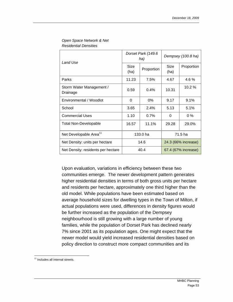
December 18, 2009


Upon evaluation, variations in efficiency between these two communities emerge. The newer development pattern generates higher residential densities in terms of both gross units per hectare and residents per hectare, approximately one third higher than the old model. While populations have been estimated based on average household sizes for dwelling types in the Town of Milton, if actual populations were used, differences in density figures would be further increased as the population of the Dempsey neighbourhood is still growing with a large number of young families, while the population of Dorset Park has declined nearly 7% since 2001 as its population ages. One might expect that the newer model would yield increased residential densities based on policy direction to construct more compact communities and its

11 Includes all internal streets.

Open Space Network & Net Residential Densities

Dorset Park (149.6 ha)

Dempsey (100.8 ha)

Land Use Size (ha)

ProportionSize (ha)

Proportion

Parks 11.23 7.5% 4.67 4.6 %

Storm Water Management / Drainage

0.59 0.4% 10.31 10.2 %

Environmental / Woodlot 0 0% 9.17 9.1%

School 3.65 2.4% 5.13 5.1%

Commercial Uses 1.10 0.7% 0 0 %

Total Non-Developable 16.57 11.1% 29.28 29.0%

Net Developable Area11 133.0 ha 71.5 ha

Net Density: units per hectare 14.6 24.3 (66% increase)

Net Density: residents per hectare 40.4 67.4 (67% increase)

December 18, 2009


smaller residential lots, and this would appear to be the case in spite of increased parkland and stormwater management provisions in this neighbourhood which reduce developable area.

If we remove all of the park and stormwater management lands from each neighbourhood and just look at the occupied blocks and streets, Dempsey still emerges, but to a greater degree. This increased provision of open space is however an important trend. The retention of woodlots and the provision of large stormwater management facilities result in significantly higher proportions of undeveloped lands than is found in the post-war neighbourhood.

The new model does however require more local infrastructure in terms of total street length per square kilometre due its more intricate street network. The higher residential densities of this neighbourhood help balance the impact of a more extensive street network, resulting nearly equal per capita rates of infrastructure provision. An assessment of the length of local streets provided both per dwelling unit and per residents are equal between the two development patterns in this case. While many theorize that the grid pattern represents a more efficient form that will reduce per capita aggregate consumption, the Milton case studies do not provide evidence to support this assumption.

Another noteworthy point to draw from this comparison is the impact of urban form on travel patterns. It is often thought that creating walkable, well connected communities will encourage residents to embrace alternative modes of travel. In this case however, despite also being adjacent to the GO station and served by the same bus routes, the new model actually has 31% fewer people that regularly utilize transit, cycling or walking to get to work. It would appear that urban form alone, at least in a suburban context, will not influence travel behaviour, and associated demand for highway or transit infrastructure, to any significant degree. In this case, the higher use of walking and transit in Dorset Park may relate to the age of the community, with a higher proportion of residents working locally rather than commuting outward (42% in Dorset Park versus only 17% in Dempsey).

Overall, it would appear that there isn’t a significant difference between the two models in terms of infrastructure efficiency and the

December 18, 2009


provision of streets on a per capita basis is roughly equal. The newer Dempsey neighbourhood is slightly more efficient in terms of use of urban land resources, but the increased provision of undeveloped open space restricts further increases in overall neighbourhood density. A more detailed assessment of these neighbourhoods based on proportional aggregate consumption rates may identify additional variations such as the impact of dwelling type mix.

Key Trends:

While the new neighbourhood pattern is more dense, this higher density is offset by a more elaborate street network. Overall, the new neighbourhood is no more efficient in terms of per capita aggregate consumption.

Through increased densities, the new neighbourhood consumes less land and better centralizes the population, creating some regional infrastructure savings.

6.3 CASE STUDY 2: REGENT PARK (INFILL / INTENSIFICATION)

This case study will assess changes in how lands are developed or redeveloped in a dense urban setting by comparing two large-scale development plans for the Regent Park area of Toronto which were established under contrasting design ideologies. This serves as a good example for how urban centres continue to evolve through the process of urban intensification and redevelopment. Further, an assessment of these contrasting plans will shed light on how approaches to planning and land management in dense urban settings has changed and what these changes mean for aggregate consumption.

The first was built in the post-war era and reflects development patterns for higher density uses most prevalent throughout the GGH until the 1990s. This form is based on the concept of segregating land uses and creating a tower-in-the-park atmosphere which seeks to maximize access to greenspace. This form of high

December 18, 2009


density development can still be found in a more limited capacity in suburban settings, but has largely fallen out of favour.

The second plan was developed only recently and is now being implemented on the site. The new development plan reintroduces a traditional urban street grid, provides a greater mix of uses and centralizes park space. This plan will almost completely replace the previous development and serves as a good example of how development projects are design today within these mixed-use, higher density urban settings.

December 18, 2009


Regent Park (1959-2005) Regent Park (under construction)

6.4 REGENT PARK: URBAN RENEWAL CONCEPT (MID-20TH CENTURY)

Regent Park covers approximately 28 hectares at the eastern edge of Downtown Toronto. The lands on which Regent Park now stand were previously home to a predominantly low-income, low-rise residential community (St. James Town) which was razed in 1948 to accommodate a substantial urban renewal scheme. This process was commonly known as “slum clearing”. All of the historic buildings and urban fabric were cleared out and replaced with an entirely different form of urban development which provided new social housing opportunities.

The Regent Park community is divided into two distinct phases by Dundas Street, which is also the only street to traverse the entire site. North Regent Park was built first between 1948 and 1957 and features a number of low-rise walk-up apartment buildings ranging in height from three to six storeys. South Regent Park followed from 1957 to 1959 and features five larger apartment towers. Clusters of townhouse dwellings are also found throughout both phases and a community centre was later added.

Regent Park was designed to be a largely self-contained community, with an internal open space system and no through traffic. The intent was to maximize views and access to open space for residents and to create a largely car-free, park-like setting. Over time however it became evident this form of development had the

December 18, 2009


effect of physically isolating Regent Park from the larger community and its highly-internalised circulation pattern and lack of permeability undermined public safety. The lack of jobs and retail uses along with the lack of diversity in terms of resident socio-economic status also contributed to the social isolation of Regent Park.

Despite being built over 50 years ago, many of the design ideals that gave rise to Regent Park as it stands today persist in higher density residential development, particularly is suburban settings, and this approach remained the accepted norm for several years until new ideologies began to take root in the 1990s. Throughout the apartment boom of the 1970s and until fairly recently, this tower-in-the-park theme was prevalent in communities throughout Ontario. Today however, a new design ideology has taken root and will again dramatically reshape the Regent Park community.

Internal walkways provide east-west connections Apartment towers in Regent Park south

Regent Park is located at the eastern edge of Downtown Dundas Street separates North and south Regent Park.

The following tables provide and overview of the development and population characteristics of Regent Park prior to the approval of redevelopment plans and phased demolition.

December 18, 2009


Housing Roads

Type of Dwelling No. % Total Length of Local Streets 2.32 km

Number of Townhome Dwellings 305 15% Total Length of Collector Streets 0.66 km

Number of Apartment Dwellings 1782 85% Length of Laneways 0 km

Total Number of Units 2087 100% Total Road Length 2.98 km


Population Characteristics (2001)

Total Population of Study Area 7,500

Average Household Size 3.6

Gross Residential Density (units per hectare) 74.3

6.4.1 Regent Park, Toronto (1950s)

December 18, 2009


Regent Park: Revitalization Plan (21st Century)

Despite the best of intentions, the Regent Park urban renewal scheme of the 1950s was found to be largely dysfunctional and in 2002 a new plan for this community was revealed which would once again see the neighbourhood razed and built anew. This process has begun and Phase 1 of the revitalization scheme is presently under construction around the intersection of Dundas and Parliament streets.

The new plan for Regent Park also features and mix of townhome and apartments with a connected open space network, but arranged very differently. The plan seeks to reintroduce the traditional urban street grid pattern in order to ‘open up’ the community and improve site permeability and circulation. Buildings will be oriented to streets rather than internal spaces and streets will also serve as the primary system of public open space in the neighbourhood. Taller buildings are proposed along major street and key focal points such as Dundas, while lower rise forms are generally anticipated along minor streets and opposite neighbouring low-rise forms. The plan features a large central park space which is flanked on all sides by public streets and will be faced by apartment dwellings to provide enhanced visibility and sense of security. Townhome units are spread through each phase of the plan and will front onto local streets.

Rear access laneways will be provided behind new development in order to hide parking and contribute to a more attractive and pedestrian-friendly streetscape free of driveways. On-street parking will be provided, but surface parking lots are not anticipated. The new plan will also incorporate limited non-residential uses including ground floor retail and professional uses along key streets such as Parliament Street and the west end of Gerrard. These non-residential uses include food stores, restaurants, retail shops and personal services.

The principal objective of the revitalization scheme is to create development that fits into the surrounding community and doesn’t appear to be a singular monolithic project. Rather, the replicated street grid, sensitive arrangement of building forms relative to neighbouring lands, and phased approach seek to create a place

December 18, 2009


that fells like any other dense urban neighbourhood and fits into the surrounding city.

Based on the Regent Park Revitalization Plan prepared for the Toronto Community Housing Corporation and the City’s approved Secondary Plan, the tables below describe the planned urban structure and anticipated population for the community when fully rebuilt. It should be noted that the revitalization plan for Regent Park is expected to take several years to fully implement and final unit counts and land use mix may vary based on market conditions. Some estimates have put the final number of residential dwellings as high as 5,900 units12, but the 4,500 units anticipated through the planning process will be used for the purpose of this analysis.

Regent Park Revitalization Plan: Building Design Concepts

Additional greenspace provided on rooftops13 Tall buildings used to anchor key intersections

12 Cheney, P. (2006); Wrecking Ball Ready. The Globe and Mail, September 11, 2006. 13 Insert source

December 18, 2009


Ground floor retail use on prominent streets Community facilities such as church are retained

Mid-rise buildings adjacent to neighbouring Cabbagetown The school and one old tower will be retained.

Housing Roads

Type of Dwelling No. % Total Length of Local Streets

2.30 km

Number of Townhome Dwellings

800 18% Total Length of

Collector Streets 2.67 km


3700 82%

Length of Laneways 3.14 km

Total Number of Units 4500

100% Total Road Length

8.10 km


Population Characteristics (2001)

Total Population of Study Area 12,500

Average Household Size 2.8

Gross Residential Density (units per hectare) 160.7

December 18, 2009


Planned Future Street Network14

6.4.2 Land Use Analysis & Area Comparisons

Two plans for Toronto’s Regent Park neighbourhood are presented, both of which involve the full-scale clearing of an urban neighbourhood in order to construct a new form of development befitting the time. While the first attempt reflected the ideals and largely accepted best practices prevalent in the post-war decades, the new plan reflects a modern approach characteristic of how higher density urban settings are planned today.

Some of the fundamental differences between these plans relate to the mixing of land uses, the organization and provision of open space, the role of streets, and the relationships between streets, parks and building. For the purpose of this study, we won’t delve

14 Toronto Community Housing (2004); Presentation: Regent Park Redevelopment

December 18, 2009


too deeply into the rationale behind these contrasting development forms, but rather will seek to identify difference is aggregate resource efficiencies which will help identify consumption trends related to the intensification of urban centres. As with the suburban case study, two key factors emerge relative to urban form: building types and street patterns.

While both plans feature a mix of apartments and townhomes, the new plan features almost exclusively taller apartment forms rather than the low-rise walk-ups featured in Regent Park north. Taller buildings generally require increased volumes and high quality aggregates for structural stability. Further, while the old plan featured surface parking lots, these new buildings apartment buildings will include underground parking facilities. It is anticipated that the new apartment dwellings will require proportionally higher volumes and quality of aggregate than the old.

The difference observed between changes in unit and population densities is a result of reduced average household sizes. While the old Regent Park featured exclusively social housing units, the new plan will introduce a near 50-50 split between subsidised and market rate. The old Regent Park featured average household sizes much greater than the City’s average of 2.5 persons per


Efficiency Measure Old Regent

Park

New Regent

Park

Proportional Difference

Gross Density : units per hectare 74.4 160.7 116%

Gross Density: residents per hectare 267.9 446.4 67%

Road Length: metres of road per km2 10,640 m 28,930 172%

Road Length: metres of road per resident

0.40 m 0.65 m 63%

Road Length: metres of road per dwelling unit

1.43 m 1.80 m 26%

December 18, 2009


dwelling15. Average household sizes are expected to decrease from 3.6 to 2.8 persons per dwelling through a more diverse housing stock.

As for streets, it has already been described how the new plan will reintroduce a tight urban grid pattern by punching several new connections through the site. These new roads will also be paralleled by laneways and service roads located to the rear of buildings. The use of grid patterns can significantly increase street frontages and improve connectivity, but results in a much more intricate circulation system. The density of roads within the new development represents a major increase over the past development, expanding the local street network nearly threefold. Despite the population of Regent Park nearly doubling, the expanded street network still results in an increased per capita provision of street infrastructure.

In addition to the aggregate required to construct new streets and buildings in Regent Park, the large increase in population will also necessitate improvements to underground servicing such as water and sewers in order to increase capacity Separate storm sewers, sanitary sewers and watermains are expected under all local streets and little of the existing servicing will remain.

Despite being constructed at a considerably lower density, the old development model for Regent Park is actually more efficient in terms of both the absolute and per capita provision of infrastructure. The inclusion of predominately mid and high-rise apartment forms with underground parking rather than low-rise walk-ups with surface lots will also have the effect of increasing per capita consumption rates for the aggregate resources used in building construction.

While the new revitalization plan for Regent Park will utilize valued urban land resources more efficiently by introducing a large increase in population density, it must be understood that this form of development will result in increased per capita aggregate

15 2006 Census, Selected Household Characteristics: City of Toronto Census Subdivision.

December 18, 2009


consumption. This increase includes both total aggregate volumes and the proportion of high quality materials.

The intensification and redevelopment of existing urban centres will continue and is expected to accelerate based on both policy direction market incentive. Many of these projects will involve the introduction of new roads and upgraded servicing, along with new building construction typically much larger than what it’s replacing. Development and redevelopment within urban centres will generally demand higher volumes and better quality of aggregate than the development patterns it replaces. This type of growth is expected to increase as a proportion all new development.

Key Trends:

While the population of Regent Park is expected to double, the length of new roads will nearly triple. With the rate of increase for new infrastructure outpacing the rate of increase for density, a corresponding increase in per capita consumption is encountered within the site.

The significant increase to density has also necessitated the replacement of water and wastewater services to increase capacity. The construction of new roads, buildings and servicing, mitigates many of the efficiencies typically associated with infilling and more close resembles a dense greenfield development.

The creation of proportionally more high-rise units will increase per capita consumption in building construction as these structures will require large volumes of high quality aggregate which includes the construction of underground parking facilities.

December 18, 2009


The more intensive clustering residential populations will reduce outward expansion pressures at the edge of the city and produce some net infrastructure savings as this form typically consumes less infrastructure per capita than suburban development.

December 18, 2009


7.0 CONCLUSIONS

There are a wide range of trends and patterns that area actively shaping how we use aggregate resources in Ontario. Many of these trends are creating new efficiencies and reducing projected demand; while other factors are at play pushing consumption upwards. It is difficult to balance the full range of factors that influence how our cities are built and managed, but key trends emerge that serve as indicators for expected development patters. In Ontario, based on projected growth and development patterns, the following key trends emerge with respect to the consumption of aggregate resources:

The population expected to growth dramatically over the next 25 years including over 3.7 million new residents within The Greater Golden Horseshoe. Ontario’s population over this period will age and average household sizes will decrease. This will demand the construction of new dwelling units at much higher rate relative to population growth and increase per capita consumption.

New neighbourhoods are being constructed more compactly and the intensification of existing urban areas is accelerating. The is a slow general shift away from the single-family home and increased construction of higher density forms including townhomes and apartments. The construction of these more compact communities and housing forms still require significant volumes of aggregate to construct and are not expected to generate reductions in per capita consumption.

Significant investment in both highway infrastructure and expansions to rapid transit systems are planned, both of which will consume significant volumes of aggregate in construction. While increased investment in public transit will take many cars of the roads, projected population growth with still result in increased overall vehicle trips. In addition to new infrastructure, Ontario’s expansive network of streets and bridges continues to age and will demand significant

December 18, 2009


ongoing repair and maintenance which will also consume large amounts of aggregate.

While there is a definite trend in Ontario to use land resources more efficiently and promote alternative modes of travel, the construction of these compact communities and dense urban centres will still require equivalent or greater volumes of aggregate to build. Although houses are getting smaller, there are fewer people living in them and many more must be built. The expansion of highway networks will continue as will ongoing maintenance and repair requirements. In all, upon consideration of the range of consumption factors, the per capita use of aggregate resources in Ontario is not expected to change to any significant degree and should remain fairly steady. It is however anticipated that demand for high quality crushed stone material will continue its trend towards increased usage.

State of the Aggregate Resource in Ontario Study...

Documents

Transcript of State of the Aggregate Resource in Ontario Study...