STATE-FEEDBACK CONTROLmocha-java.uccs.edu/ECE5520/ECE5520-CH06.pdf · 1 Ck 2 D 30; or;k 2 D 57: ......
30
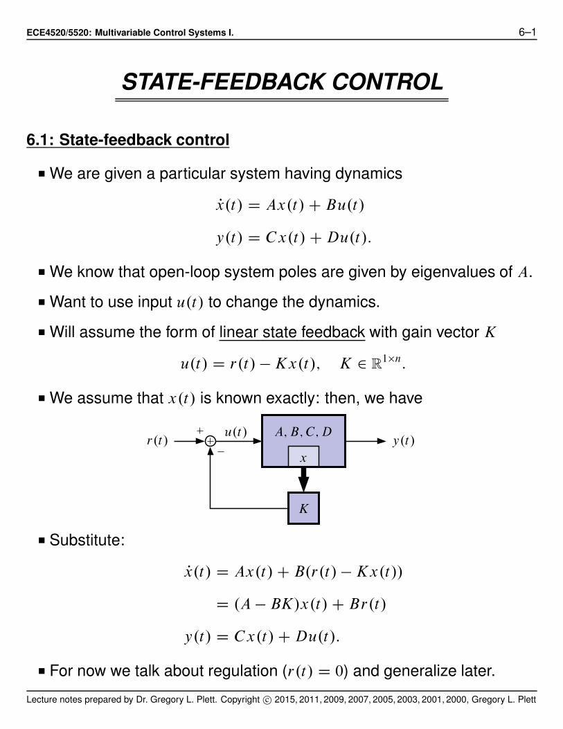
ECE4520/5520: Multivariable Control Systems I. 6–1 STATE-FEEDBACK CONTROL 6.1: State-feedback control ■ We are given a particular system having dynamics P x.t/ D Ax.t/ C Bu.t/ y.t/ D Cx.t/ C Du.t/: ■ We know that open-loop system poles are given by eigenvalues of A. ■ Want to use input u.t/ to change the dynamics. ■ Will assume the form of linear state feedback with gain vector K u.t/ D r.t/ Kx.t/; K 2 R 1n : ■ We assume that x.t/ is known exactly: then, we have r.t/ y.t/ u.t/ A;B;C;D x K ■ Substitute: P x.t/ D Ax.t/ C B.r.t/ Kx.t// D .A BK/x.t/ C Br.t/ y.t/ D Cx.t/ C Du.t/: ■ For now we talk about regulation (r.t/ D 0) and generalize later. Lecture notes prepared by Dr. Gregory L. Plett. Copyright c 2015, 2011, 2009, 2007, 2005, 2003, 2001, 2000, Gregory L. Plett
Transcript of STATE-FEEDBACK CONTROLmocha-java.uccs.edu/ECE5520/ECE5520-CH06.pdf · 1 Ck 2 D 30; or;k 2 D 57: ......
ECE4520/5520: Multivariable Control Systems I. 6–1
STATE-FEEDBACK CONTROL
6.1: State-feedback control
■ We are given a particular system having dynamics
Px.t/ D Ax.t/ C Bu.t/
y.t/ D Cx.t/ C Du.t/:
■ We know that open-loop system poles are given by eigenvalues of A.
■ Want to use input u.t/ to change the dynamics.
■ Will assume the form of linear state feedback with gain vector K
u.t/ D r.t/ ! Kx.t/; K 2 R1"n:
■ We assume that x.t/ is known exactly: then, we have
r.t/ y.t/u.t/ A; B; C; D
x
K
■ Substitute:
Px.t/ D Ax.t/ C B.r.t/ ! Kx.t//
D .A ! BK/x.t/ C Br.t/
y.t/ D Cx.t/ C Du.t/:
■ For now we talk about regulation (r.t/ D 0) and generalize later.
Lecture notes prepared by Dr. Gregory L. Plett. Copyright c# 2015, 2011, 2009, 2007, 2005, 2003, 2001, 2000, Gregory L. Plett

ECE4520/5520, STATE-FEEDBACK CONTROL 6–2
■ For now we consider SISO systems, and generalize later.
OBJECTIVE: Design K so that ACL D A ! BK has some nice properties.
For example,
■ Perhaps A is unstable. Design ACL to be stable.
■ Or, might want to put two poles at !2 ˙ j . (Pole placement.)
■ There are n parameters in the gain vector K and n eigenvalues of A.
So, what can we achieve?
EXAMPLE: Consider the (unstable) system
Px.t/ D
"
1 1
1 2
#
x.t/ C
"
1
0
#
u.t/:
det.sI ! A/ D .s ! 1/.s ! 2/ ! 1 D s2 ! 3s C 1:
■ Let
u.t/ D !h
k1 k2
i
x.t/ D !Kx.t/
ACL D A ! BK D
"
1 1
1 2
#
!
"
1
0
#h
k1 k2
i
D
"
1 ! k1 1 ! k2
1 2
#
:
■ So, det.sI ! ACL/ D s2 C .k1 ! 3/s C .1 ! 2k1 C k2/.
■ By choosing k1 and k2, we can put eig.ACL/ anywhere in the complex
plane (in complex-conjugate pairs, that is!)
■ For example, how can we place poles at !5; !6?
Lecture notes prepared by Dr. Gregory L. Plett. Copyright c# 2015, 2011, 2009, 2007, 2005, 2003, 2001, 2000, Gregory L. Plett
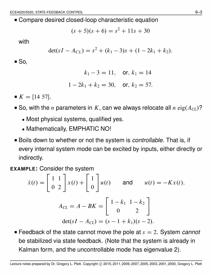
ECE4520/5520, STATE-FEEDBACK CONTROL 6–3
■ Compare desired closed-loop characteristic equation
.s C 5/.s C 6/ D s2 C 11s C 30
with
det.sI ! ACL/ D s2 C .k1 ! 3/s C .1 ! 2k1 C k2/:
■ So,
k1 ! 3 D 11; or; k1 D 14
1 ! 2k1 C k2 D 30; or; k2 D 57:
■ K D Œ14 57!.
■ So, with the n parameters in K, can we always relocate all n eig.ACL/?
$ Most physical systems, qualified yes.
$ Mathematically, EMPHATIC NO!
■ Boils down to whether or not the system is controllable. That is, if
every internal system mode can be excited by inputs, either directly or
indirectly.
EXAMPLE: Consider the system
Px.t/ D
"
1 1
0 2
#
x.t/ C
"
1
0
#
u.t/ and u.t/ D !Kx.t/:
ACL D A ! BK D
"
1 ! k1 1 ! k2
0 2
#
det.sI ! ACL/ D .s ! 1 C k1/.s ! 2/:
■ Feedback of the state cannot move the pole at s D 2. System cannot
be stabilized via state feedback. (Note that the system is already in
Kalman form, and the uncontrollable mode has eigenvalue 2).
Lecture notes prepared by Dr. Gregory L. Plett. Copyright c# 2015, 2011, 2009, 2007, 2005, 2003, 2001, 2000, Gregory L. Plett
ECE4520/5520, STATE-FEEDBACK CONTROL 6–4
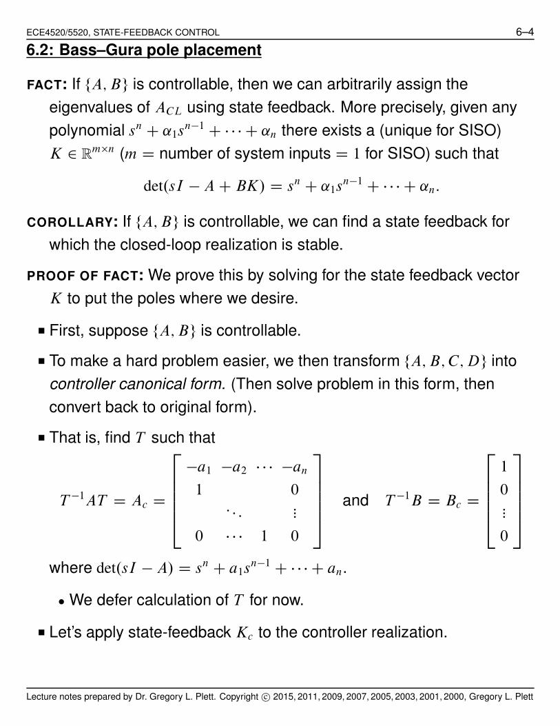
6.2: Bass–Gura pole placement
FACT: If fA; Bg is controllable, then we can arbitrarily assign the
eigenvalues of ACL using state feedback. More precisely, given any
polynomial sn C ˛1sn!1 C % % % C ˛n there exists a (unique for SISO)
K 2 Rm"n (m D number of system inputs D 1 for SISO) such that
det.sI ! A C BK/ D sn C ˛1sn!1 C % % % C ˛n:
COROLLARY: If fA; Bg is controllable, we can find a state feedback for
which the closed-loop realization is stable.
PROOF OF FACT: We prove this by solving for the state feedback vector
K to put the poles where we desire.
■ First, suppose fA; Bg is controllable.
■ To make a hard problem easier, we then transform fA; B; C; Dg into
controller canonical form. (Then solve problem in this form, then
convert back to original form).
■ That is, find T such that
T !1AT D Ac D
2
66664
!a1 !a2 % % % !an
1 0: : : :::
0 % % % 1 0
3
77775
and T !1B D Bc D
2
66664
1
0:::
0
3
77775
where det.sI ! A/ D sn C a1sn!1 C % % % C an.
$ We defer calculation of T for now.
■ Let’s apply state-feedback Kc to the controller realization.
Lecture notes prepared by Dr. Gregory L. Plett. Copyright c# 2015, 2011, 2009, 2007, 2005, 2003, 2001, 2000, Gregory L. Plett

ECE4520/5520, STATE-FEEDBACK CONTROL 6–5
■ Note, Kc Dh
k1 % % % kn
i
, so
BcKc D
2
66664
k1 k2 % % % kn
0 0::: :::
0 0
3
77775
:
■ Useful because characteristic equation obvious.
ACL D Ac ! BcKc D
2
66664
!.a1 C k1/ !.a2 C k2/ % % % !.an C kn/
1 0: : : :::
0 % % % 1 0
3
77775
;
still in controller form!
y.t/
u.t/x1c x2c x3cRR R
b1
b2
b3
!a1
!a2
!a3
!k1
!k2
!k3
■ Thus, after state feedback with Kc the characteristic equation is
det.sI ! Ac C BcKc/ D sn C .a1 C k1/sn!1 C % % % C .an C kn/:
Lecture notes prepared by Dr. Gregory L. Plett. Copyright c# 2015, 2011, 2009, 2007, 2005, 2003, 2001, 2000, Gregory L. Plett

ECE4520/5520, STATE-FEEDBACK CONTROL 6–6
■ The desired characteristic equation is
"d.s/ D sn C ˛1sn!1 C % % % C ˛n:
■ Equating coefficients of powers-of-s, we set
k1 D ˛1 ! a1; : : : ; kn D ˛n ! an and get the desired characteristic
polynomial.
■ Now that we have the solution in the controller canonical form, we
transform back to the original realization
"d.s/ D det.sI ! Ac C BcKc/
D det.T / det.sI ! Ac C BcKc/ det.T !1/
D det.sI ! TAcT!1 C TBcKcT
!1/
D det.sI ! A C BKcT!1/:
".s/ D det.sI ! A C BK/ so
K D KcT!1:
So, if we use state feedback
K D KcT!1
Dh
.˛1 ! a1/ % % % .˛n ! an/i
T !1
we will have the desired characteristic polynomial.
■ One remaining question: What is T ? We know T D CC!1c and
Cc D
2
66664
1 !a1 a21 ! a2 % % %
0 1 !a1 0::: 1 :::
0 % % % 1
3
77775
Lecture notes prepared by Dr. Gregory L. Plett. Copyright c# 2015, 2011, 2009, 2007, 2005, 2003, 2001, 2000, Gregory L. Plett
ECE4520/5520, STATE-FEEDBACK CONTROL 6–7
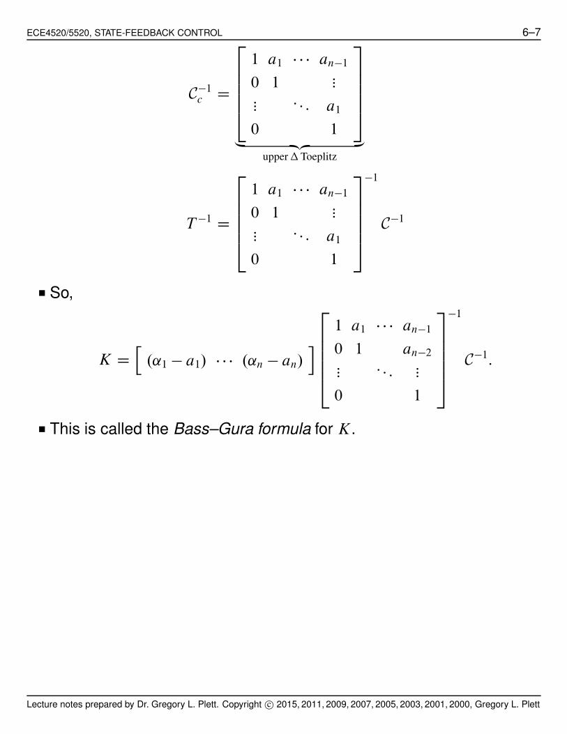
C!1c D
2
66664
1 a1 % % % an!1
0 1 :::::: : : : a1
0 1
3
77775
„ ƒ‚ …
upper # Toeplitz
T !1 D
2
66664
1 a1 % % % an!1
0 1 :::::: : : : a1
0 1
3
77775
!1
C!1
■ So,
K Dh
.˛1 ! a1/ % % % .˛n ! an/i
2
66664
1 a1 % % % an!1
0 1 an!2::: : : : :::
0 1
3
77775
!1
C!1:
■ This is called the Bass–Gura formula for K.
Lecture notes prepared by Dr. Gregory L. Plett. Copyright c# 2015, 2011, 2009, 2007, 2005, 2003, 2001, 2000, Gregory L. Plett
ECE4520/5520, STATE-FEEDBACK CONTROL 6–8
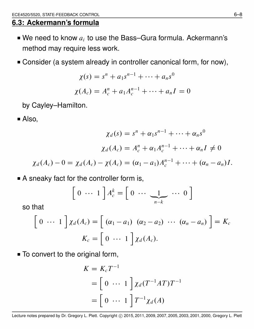
6.3: Ackermann’s formula
■ We need to know ai to use the Bass–Gura formula. Ackermann’s
method may require less work.
■ Consider (a system already in controller canonical form, for now),
".s/ D sn C a1sn!1 C % % % C ans0
".Ac/ D Anc C a1A
n!1c C % % % C anI D 0
by Cayley–Hamilton.
■ Also,
"d.s/ D sn C ˛1sn!1 C % % % C ˛ns0
"d.Ac/ D Anc C ˛1A
n!1c C % % % C ˛nI ¤ 0
"d.Ac/ ! 0 D "d.Ac/ ! ".Ac/ D .˛1 ! a1/An!1c C % % % C .˛n ! an/I:
■ A sneaky fact for the controller form is,h
0 % % % 1i
Akc D
h
0 % % % 1„ƒ‚…
n!k
% % % 0i
so thath
0 % % % 1i
"d.Ac/ Dh
.˛1 ! a1/ .˛2 ! a2/ % % % .˛n ! an/i
D Kc
Kc Dh
0 % % % 1i
"d .Ac/:
■ To convert to the original form,
K D KcT!1
Dh
0 % % % 1i
"d.T !1AT /T !1
Dh
0 % % % 1i
T !1"d.A/
Lecture notes prepared by Dr. Gregory L. Plett. Copyright c# 2015, 2011, 2009, 2007, 2005, 2003, 2001, 2000, Gregory L. Plett

ECE4520/5520, STATE-FEEDBACK CONTROL 6–9
Dh
0 % % % 1i
CcC!1"d.A/
Dh
0 % % % 1i
C!1"d.A/:
■ Revisit previous example. "d.s/ D s2 C 11s C 30.
C D
"
1 1
0 1
#
K Dh
0 1i
"
1 !1
0 1
# ( "
1 1
1 2
# "
1 1
1 2
#
C 11
"
1 1
1 2
#
C 30
"
1 0
0 1
#)
Dh
0 1i
( "
2 3
3 5
#
C
"
41 11
11 52
#)
Dh
0 1i
"
43 14
14 57
#
Dh
14 57i
: ✓ same as before:
■ K=acker(A,B,poles); ➠ Very easy in Matlab, but numerical
issues.
■ K=place(A,B,poles); ➠ Use this instead, unless you have
repeated roots.
■ polyvalm.m ➠ To compute "d.A/.
Simulating state feedback in Simulink
■ The following block diagram may be used to simulate a
state-feedback control system in Simulink.
Lecture notes prepared by Dr. Gregory L. Plett. Copyright c# 2015, 2011, 2009, 2007, 2005, 2003, 2001, 2000, Gregory L. Plett

ECE4520/5520, STATE-FEEDBACK CONTROL 6–10
Note: All (square) gain blocks are MATRIX GAIN blocks
from the Math Library.
1y
K
K
s1
K
D
K
C
K
BK
A
1r
xdot xu
Some comments
FACT: The eigenvalues associated with uncontrollable modes are fixed
(don’t change) under state feedback, but those associated with
controllable modes can be arbitrarily assigned.
FACT: State feedback does not change zeros of a realization.
FACT: Drastic changes in characteristic polynomial requires large gains
K (high control effort).
FACT: State feedback can result in unobservable modes (pole-zero
cancellations).
Lecture notes prepared by Dr. Gregory L. Plett. Copyright c# 2015, 2011, 2009, 2007, 2005, 2003, 2001, 2000, Gregory L. Plett
ECE4520/5520, STATE-FEEDBACK CONTROL 6–11
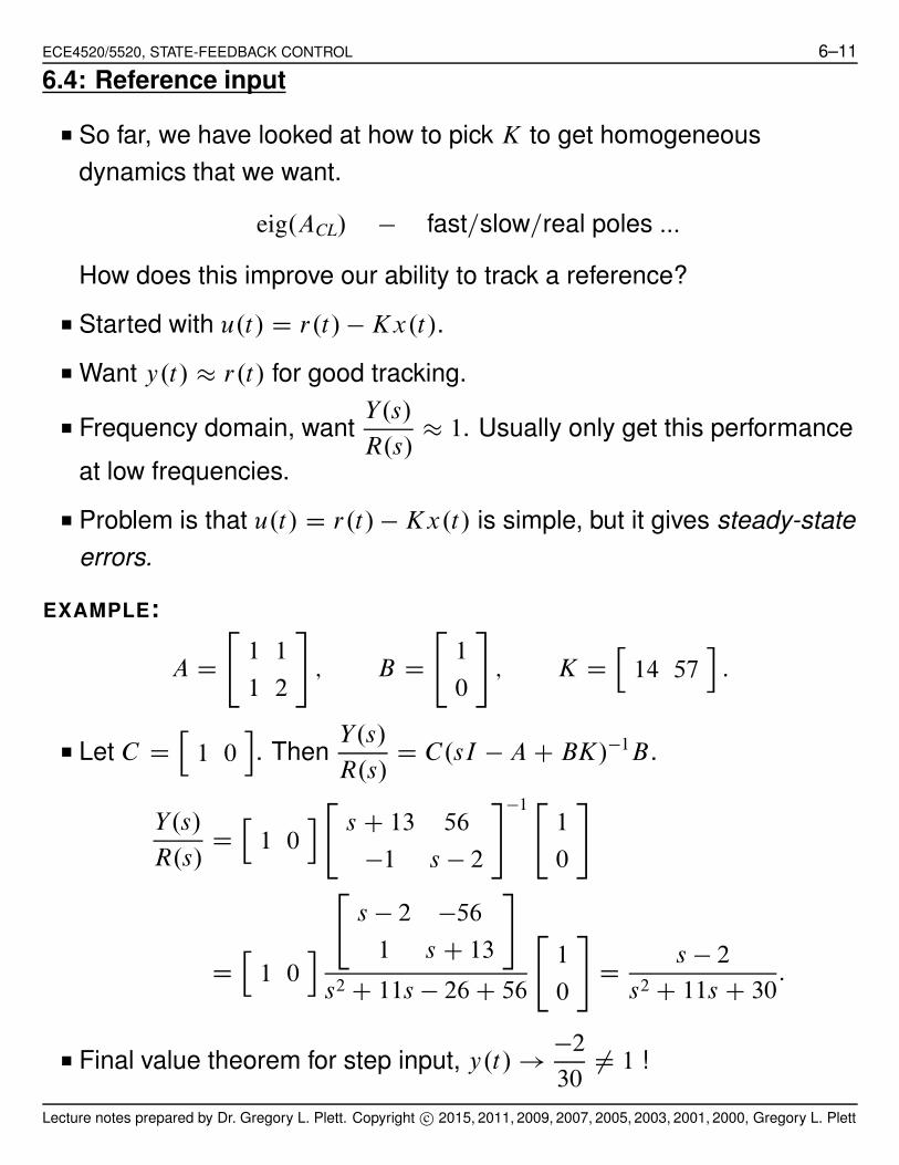
6.4: Reference input
■ So far, we have looked at how to pick K to get homogeneous
dynamics that we want.
eig.ACL/ ! fast=slow=real poles :::
How does this improve our ability to track a reference?
■ Started with u.t/ D r.t/ ! Kx.t/.
■ Want y.t/ & r.t/ for good tracking.
■ Frequency domain, wantY.s/
R.s/& 1. Usually only get this performance
at low frequencies.
■ Problem is that u.t/ D r.t/ ! Kx.t/ is simple, but it gives steady-state
errors.
EXAMPLE:
A D
"
1 1
1 2
#
; B D
"
1
0
#
; K Dh
14 57i
:
■ Let C Dh
1 0i
. ThenY.s/
R.s/D C.sI ! A C BK/!1B.
Y.s/
R.s/D
h
1 0i
"
s C 13 56
!1 s ! 2
#!1 "
1
0
#
Dh
1 0i
"
s ! 2 !56
1 s C 13
#
s2 C 11s ! 26 C 56
"
1
0
#
Ds ! 2
s2 C 11s C 30:
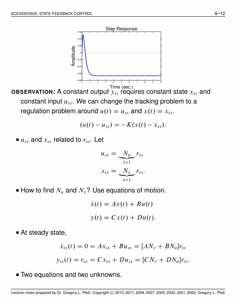
■ Final value theorem for step input, y.t/ !!2
30¤ 1 !
Lecture notes prepared by Dr. Gregory L. Plett. Copyright c# 2015, 2011, 2009, 2007, 2005, 2003, 2001, 2000, Gregory L. Plett
ECE4520/5520, STATE-FEEDBACK CONTROL 6–12
0 1 2 3 4 5 6 7 8 9 10−0.08
−0.06
−0.04
−0.02
0
0.02
0.04
0.06Step Response
Am
plit
ude
Time (sec.)OBSERVATION: A constant output yss requires constant state xss and
constant input uss. We can change the tracking problem to a
regulation problem around u.t/ D uss and x.t/ D xss.
.u.t/ ! uss/ D !K.x.t/ ! xss/:
■ uss and xss related to rss. Let
uss D Nu„ƒ‚…
1"1
rss
xss D Nx„ƒ‚…
n"1
rss:
■ How to find Nu and Nx? Use equations of motion.
Px.t/ D Ax.t/ C Bu.t/
y.t/ D Cx.t/ C Du.t/:
■ At steady state,
Pxss.t/ D 0 D Axss C Buss D ŒANx C BNu!rss
yss.t/ D rss D Cxss C Duss D ŒCNx C DNu!rss:
■ Two equations and two unknowns.
Lecture notes prepared by Dr. Gregory L. Plett. Copyright c# 2015, 2011, 2009, 2007, 2005, 2003, 2001, 2000, Gregory L. Plett
ECE4520/5520, STATE-FEEDBACK CONTROL 6–13
"
A B
C D
# "
Nx
Nu
#
D
"
0
I
#
:
■ In steady-state we had
.u.t/ ! uss/ D !K.x.t/ ! xss/
which is achieved by the control signal
u.t/ D Nur.t/ ! K.x.t/ ! Nxr.t//
D !Kx.t/ C .Nu C KNx/r.t/
D !Kx.t/ C NN r.t/:
■ NN computed without knowing r.t/. It works for any r.t/.
■ In our example we can find that
"
Nx
Nu
#
D
2
64
1
!1=2
!1=2
3
75 :
■ Nu C KNx D !15:
■ New equations:
Px.t/ D Ax.t/ C B.Nu C KNx/r.t/ ! BKx.t/
D .A ! BK/x.t/ C B NN r.t/
y.t/ D Cx.t/:
■ Therefore,!
Y.s/
R.s/
"
new
D
!
Y.s/
R.s/
"
old
" NN D!15s C 30
s2 C 11s C 30
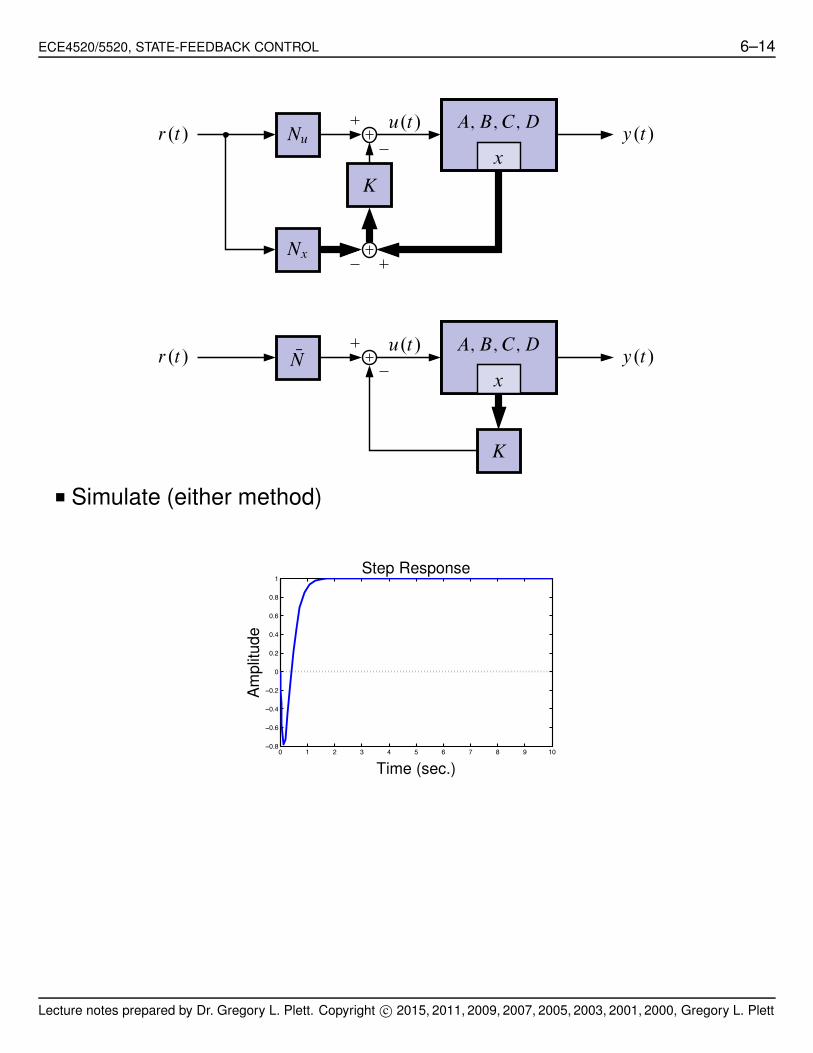
which has zero steady-state error to a unit-step.
Lecture notes prepared by Dr. Gregory L. Plett. Copyright c# 2015, 2011, 2009, 2007, 2005, 2003, 2001, 2000, Gregory L. Plett
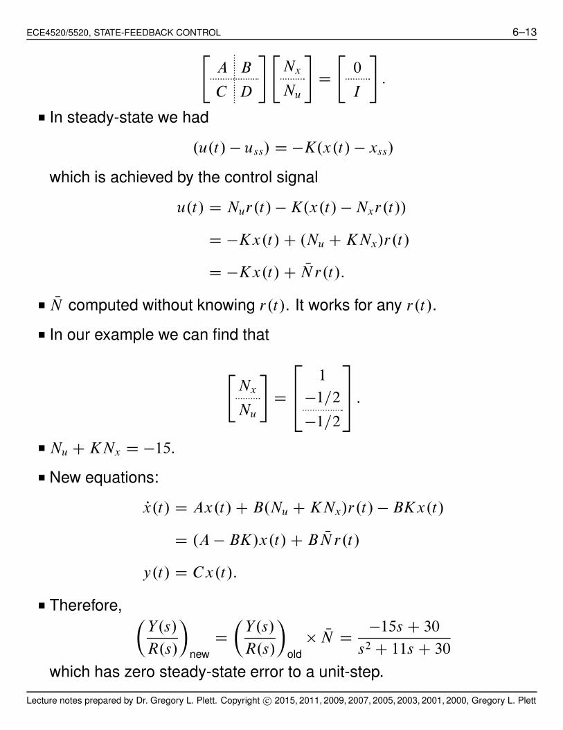
ECE4520/5520, STATE-FEEDBACK CONTROL 6–14
r.t/
r.t/
y.t/
y.t/
u.t/
u.t/
A; B; C; D
A; B; C; D
x
x
K
K
NN
Nx
Nu
■ Simulate (either method)
0 1 2 3 4 5 6 7 8 9 10−0.8
−0.6
−0.4
−0.2
0
0.2
0.4
0.6
0.8
1Step Response
Am
plit
ude
Time (sec.)
Lecture notes prepared by Dr. Gregory L. Plett. Copyright c# 2015, 2011, 2009, 2007, 2005, 2003, 2001, 2000, Gregory L. Plett
ECE4520/5520, STATE-FEEDBACK CONTROL 6–15
6.5: Pole placement
■ Classical question: Where do we place the closed-loop poles?
THOUGHT I: Dominant second-order behavior, just as before.
■ Assume dominant behavior given by roots of
s2 C 2$!ns C !2n ➠ s D !
n
!n ˙ j!n
p
1 ! $2o
■ Put other poles so that the time response is much faster than this
dominant behavior.
■ Place them so that they are “sufficiently damped.”
$ Real part < !4$!n.
$ Keep frequency same as open loop.
■ Be very careful about moving poles too far. Takes a lot of control
effort.
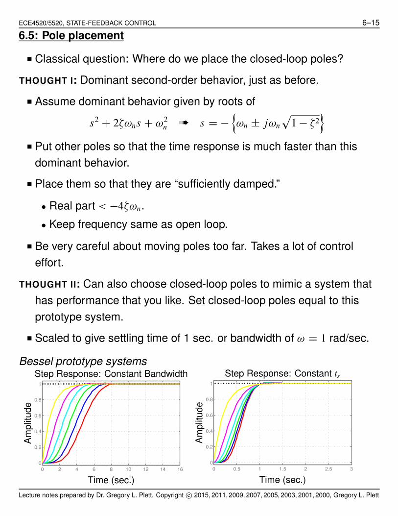
THOUGHT II: Can also choose closed-loop poles to mimic a system that
has performance that you like. Set closed-loop poles equal to this
prototype system.
■ Scaled to give settling time of 1 sec. or bandwidth of ! D 1 rad/sec.
Bessel prototype systems
0 2 4 6 8 10 12 14 160
0.2
0.4
0.6
0.8
1
Time (sec.)
Am
plit
ude
Step Response: Constant Bandwidth
0 0.5 1 1.5 2 2.5 30
0.2
0.4
0.6
0.8
1
Time (sec.)
Am
plit
ude
Step Response: Constant ts
Lecture notes prepared by Dr. Gregory L. Plett. Copyright c# 2015, 2011, 2009, 2007, 2005, 2003, 2001, 2000, Gregory L. Plett

ECE4520/5520, STATE-FEEDBACK CONTROL 6–16
ITAE prototype systems
0 2 4 6 8 10 12 14 160
0.2
0.4
0.6
0.8
1
Time (sec.)
Am
plit
ude
Step Response: Constant Bandwidth
0 0.5 1 1.5 2 2.5 30
0.2
0.4
0.6
0.8
1
Time (sec.)
Am
plit
ude
Step Response: Constant ts
PROCEDURE: For nth-order system—desired bandwidth.
1. Determine desired bandwidth !o.
2. Find the nth-order poles from the table of constant bandwidth, and
multiply pole locations by !o.
3. Use Acker/place to locate poles. Simulate and check control effort.
PROCEDURE: For nth-order system—desired settling time.
1. Determine desired settling time ts.
2. Find the nth-order poles from the table of constant settling time,
and divide pole locations by ts.
3. Use Acker/place to locate poles. Simulate and check control effort.
■ Bessel model has no overshoot, but is slow compared with ITAE.
■ NOT a good idea for flexible systems. Why?
Lecture notes prepared by Dr. Gregory L. Plett. Copyright c# 2015, 2011, 2009, 2007, 2005, 2003, 2001, 2000, Gregory L. Plett

EC
E4520/5
520,
STA
TE
-FE
ED
BA
CK
CO
NT
RO
L6–17
ITAE pole locations for ts D 1 sec.
1: !4:620
2: !4:660 ˙ 4:660j
3: !4:350 ˙ 8:918j !5:913
4: !4:236 ˙ 12:617j !6:254 ˙ 4:139j
5: !3:948 ˙ 13:553j !6:040 ˙ 5:601j !9:394
6: !2:990 ˙ 12:192j !5:602 ˙ 7:554j !7:089 ˙ 2:772j
Bessel pole locations for ts D 1 sec.
1: !4:620
2: !4:053 ˙ 2:340j
3: !3:967 ˙ 3:785j !5:009
4: !4:016 ˙ 5:072j !5:528 ˙ 1:655j
5: !4:110 ˙ 6:314j !5:927 ˙ 3:081j !6:448
6: !4:217 ˙ 7:530j !6:261 ˙ 4:402j !7:121 ˙ 1:454j
ITAE pole locations for !o D 1 rad/sec.
1: !1:000
2: !0:707 ˙ 0:707j
3: !0:521 ˙ 1:068j !0:708
4: !0:424 ˙ 1:263j !0:626 ˙ 0:414j
5: !0:376 ˙ 1:292j !0:576 ˙ 0:534j !0:896
6: !0:310 ˙ 0:962j !0:581 ˙ 0:783j !0:735 ˙ 0:287j
Bessel pole locations for !o D 1 rad/sec.
1: !1:000
2: !0:866 ˙ 0:500j
3: !0:746 ˙ 0:711j !0:942
4: !0:657 ˙ 0:830j !0:905 ˙ 0:271j
5: !0:591 ˙ 0:907j !0:852 ˙ 0:443j !0:926
6: !0:539 ˙ 0:962j !0:800 ˙ 0:562j !0:909 ˙ 0:186j
Lectu
renote
spre
pare
dby
Dr.
Gre
gory
L.P
lett.
Copyrig
ht
c#2015,2
011,2
009,2
007,2
005,2
003,2
001,2
000,
Gre
gory
L.
Ple
tt
ECE4520/5520, STATE-FEEDBACK CONTROL 6–18
10−1 100 101−140
−120
−100
−80
−60
−40
−20
0ITAE: –, Bessel, ’––’
Magnitu
de
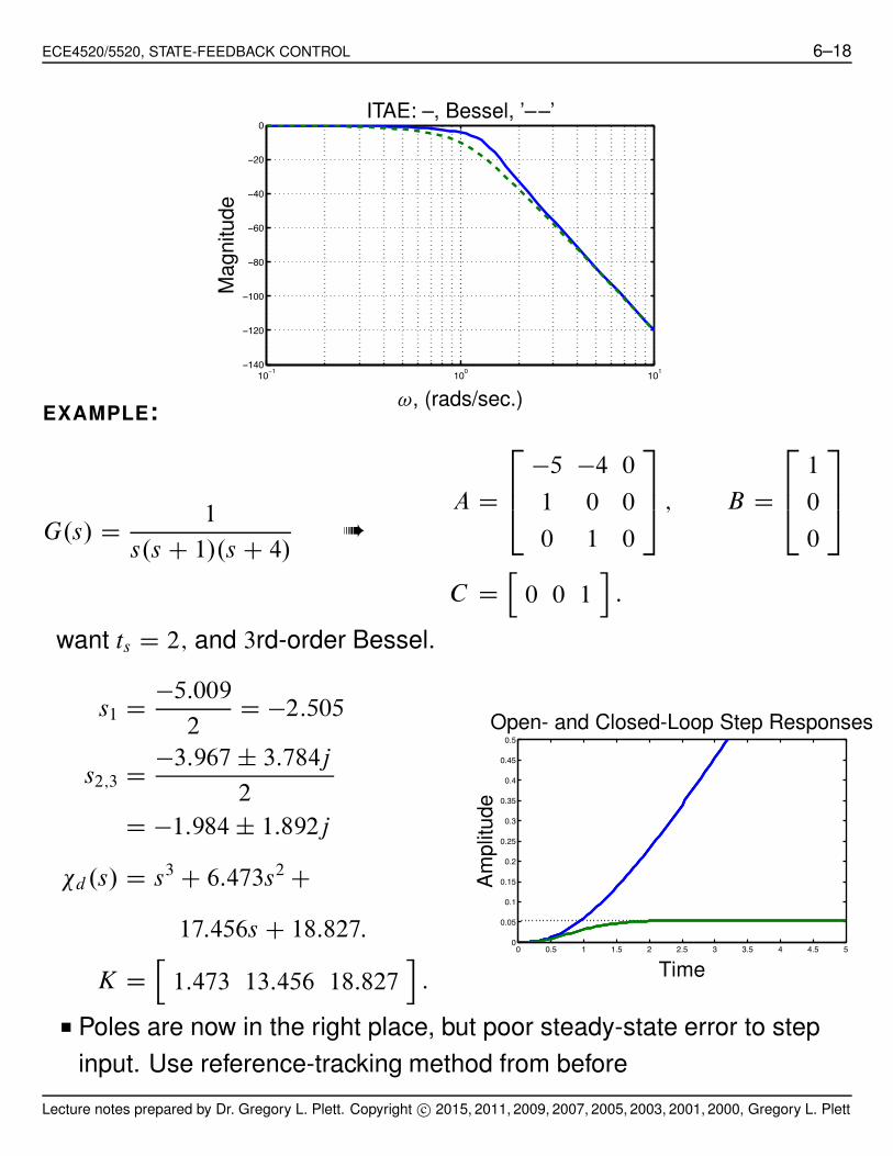
!, (rads/sec.)EXAMPLE:
G.s/ D1
s.s C 1/.s C 4/➠
A D
2
64
!5 !4 0
1 0 0
0 1 0
3
75 ; B D
2
64
1
0
0
3
75
C Dh
0 0 1i
:
want ts D 2; and 3rd-order Bessel.
s1 D!5:009
2D !2:505
s2;3 D!3:967 ˙ 3:784j
2
D !1:984 ˙ 1:892j
"d.s/ D s3 C 6:473s2 C
17:456s C 18:827:
K Dh
1:473 13:456 18:827i
:
0 0.5 1 1.5 2 2.5 3 3.5 4 4.5 50
0.05
0.1
0.15
0.2
0.25
0.3
0.35
0.4
0.45
0.5
Time
Am
plit
ude
Open- and Closed-Loop Step Responses
■ Poles are now in the right place, but poor steady-state error to step
input. Use reference-tracking method from before
Lecture notes prepared by Dr. Gregory L. Plett. Copyright c# 2015, 2011, 2009, 2007, 2005, 2003, 2001, 2000, Gregory L. Plett
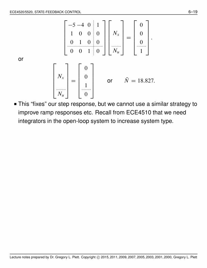
ECE4520/5520, STATE-FEEDBACK CONTROL 6–19
2
66664
!5 !4 0 1
1 0 0 0
0 1 0 0
0 0 1 0
3
77775
2
66664
Nx
Nu
3
77775
D
2
66664
0
0
0
1
3
77775
:
or2
66664
Nx
Nu
3
77775
D
2
66664
0
0
1
0
3
77775
or NN D 18:827:
■ This “fixes” our step response, but we cannot use a similar strategy to
improve ramp responses etc. Recall from ECE4510 that we need
integrators in the open-loop system to increase system type.
Lecture notes prepared by Dr. Gregory L. Plett. Copyright c# 2015, 2011, 2009, 2007, 2005, 2003, 2001, 2000, Gregory L. Plett

ECE4520/5520, STATE-FEEDBACK CONTROL 6–20
6.6: Integral control for continuous-time systems
■ In many practical designs, integral control is needed to counteract
disturbances, plant variations, or other noises in the system.
■ Up until now, we have not seen a design that has integral action. In
fact state-space designs will NOT produce integral action unless we
make special steps to include it!
■ How do we introduce integral control? We augment our system with
one or more integrators:
r.t/ y.t/u.t/xI .t/ A; B; C; D
x
Kx
KI1
s
■ In other words, include an integral state equation of
PxI .t/ D r.t/ ! y.t/
D r.t/ ! .Cx.t/ C Du.t//:
and THEN design KI and Kx such that the system had good
closed-loop pole locations.
■ Note that we can include the integral state into our normal
state-space form by augmenting the system dynamics
"
PxI .t/
Px.t/
#
D
"
0 !C
0 A
# "
xI .t/
x.t/
#
C
"
!D
B
#
u.t/ C
"
I
0
#
r.t/
y.t/ D Cx.t/ C Du.t/:
Lecture notes prepared by Dr. Gregory L. Plett. Copyright c# 2015, 2011, 2009, 2007, 2005, 2003, 2001, 2000, Gregory L. Plett
ECE4520/5520, STATE-FEEDBACK CONTROL 6–21
■ Note that the matrix that now fills the state-space placeholder usually
called “A” has an open-loop eigenvalue at the origin. This
corresponds to increasing the system type, and integrates out
steady-state error.
■ The control law is,
u.t/ D !h
KI Kx
i"
xI .t/
x.t/
#
:
■ This is state feedback on the augmented state vector. We can find the
feedback gain vector K by using Ackerman’s formula (or similar) by
replacing “A” in Ackerman with the augmented “A” matrix above, and
by replacing “B” in Ackerman by the matrix multiplying u.t/ above.
■ Note that the augmented system has n C nI open-loop poles, so we
will have to choose n C nI desired closed-loop poles, and split the
resulting K into the parts KI and Kx.
■ When we substitute the control law for u.t/ into the open-loop
augmented state-space dynamics, we get:
"
PxI .t/
Px.t/
#
D
0
BBBB@
ACL‚ …„ ƒ"
0 !C
0 A
#
„ ƒ‚ …
A in Acker/place
!
"
!D
B
#
„ ƒ‚ …
B in Acker/place
h
KI Kx
i
1
CCCCA
"
xI .t/
x.t/
#
C
"
I
0
#
r.t/
■ This is a state-space system with the augmented state vector, and
input r.t/.
■ Our previous example becomes:
Lecture notes prepared by Dr. Gregory L. Plett. Copyright c# 2015, 2011, 2009, 2007, 2005, 2003, 2001, 2000, Gregory L. Plett
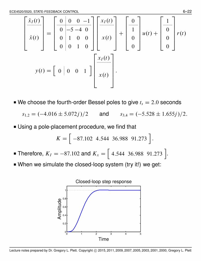
ECE4520/5520, STATE-FEEDBACK CONTROL 6–222
66664
PxI .t/
Px.t/
3
77775
D
2
66664
0 0 0 !1
0 !5 !4 0
0 1 0 0
0 0 1 0
3
77775
2
66664
xI .t/
x.t/
3
77775
C
2
66664
0
1
0
0
3
77775
u.t/ C
2
66664
1
0
0
0
3
77775
r.t/
y.t/ Dh
0 0 0 1i
2
66664
xI .t/
x.t/
3
77775
:
■ We choose the fourth-order Bessel poles to give ts D 2:0 seconds
s1;2 D .!4:016 ˙ 5:072j /=2 and s3;4 D .!5:528 ˙ 1:655j /=2:
■ Using a pole-placement procedure, we find that
K Dh
!87:102 4:544 36:988 91:273i
:
■ Therefore, KI D !87:102 and Kx Dh
4:544 36:988 91:273i
.
■ When we simulate the closed-loop system (try it!) we get:
0 1 2 3 4 50
0.2
0.4
0.6
0.8
1
Time
Am
plit
ude
Closed-loop step response
Lecture notes prepared by Dr. Gregory L. Plett. Copyright c# 2015, 2011, 2009, 2007, 2005, 2003, 2001, 2000, Gregory L. Plett

ECE4520/5520, STATE-FEEDBACK CONTROL 6–23
6.7: State feedback for discrete-time systems
■ The result is identical.
Characteristic frequencies of controllable modes are freely
assignable by state feedback; characteristic frequencies of
uncontrollable modes do not change with state feedback.
■ There is a special characteristic polynomial for discrete-time systems
".´/ D ´nI
that is, all eigenvalues are zero.
■ What does this mean? By Cayley-Hamilton,
.A ! BK/n D 0:
■ Hence, with no input, the state reaches 0 in at most n steps since
xŒn! D .A ! BK/nxŒ0! D 0
no matter what xŒ0! is.
■ This is called dead-beat control and A ! BK is called a Nilpotent
matrix.
EXAMPLE: Consider
xŒk C 1! D
"
1 0
2 2
#
xŒk! C
"
1
0
#
uŒk!:
■ This system is controllable, so we can find a K D Œk1 k2! such that
det
"
´ ! 1 C k1 k2
!2 ´ ! 2
#
D ´2
.´ ! 1 C k1/.´ ! 2/ C 2k2 D
Lecture notes prepared by Dr. Gregory L. Plett. Copyright c# 2015, 2011, 2009, 2007, 2005, 2003, 2001, 2000, Gregory L. Plett

ECE4520/5520, STATE-FEEDBACK CONTROL 6–24
and therefore k1 D 3 and k2 D 2.
A ! BK D
"
!2 !2
2 2
#
.A ! BK/2 D
"
0 0
0 0
#
as claimed:
■ The open-loop system is unstable, but the closed-loop system is not
only stable but effects of initial conditions completely disappear after
two time steps–they do not merely decay.
■ This is a common design procedure, but beware of high control effort.
Reference input
■ Tracking a reference input with a discrete-time system requires the
same method as for continuous-time systems.
Integral control
■ Again, we augment our system with a (discrete-time) integrator:
rŒk! yŒk!uŒk! A; B; C; D
x
Kx
´!1
Integrator
xI Œk!
xI Œk C 1!
KI
■ In discrete time, we include an integral state equation of
xI Œk C 1! D xI Œk! C rŒk! ! yŒk!
D xI Œk! C rŒk! ! .CxŒk! C DuŒk!/:
Lecture notes prepared by Dr. Gregory L. Plett. Copyright c# 2015, 2011, 2009, 2007, 2005, 2003, 2001, 2000, Gregory L. Plett
ECE4520/5520, STATE-FEEDBACK CONTROL 6–25
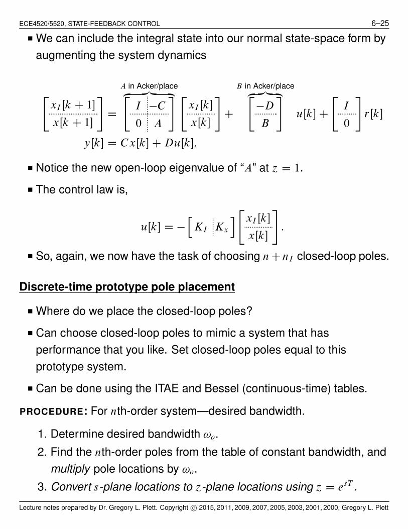
■ We can include the integral state into our normal state-space form by
augmenting the system dynamics
"
xI Œk C 1!
xŒk C 1!
#
D
A in Acker/place‚ …„ ƒ"
I !C
0 A
# "
xI Œk!
xŒk!
#
C
B in Acker/place‚ …„ ƒ"
!D
B
#
uŒk! C
"
I
0
#
rŒk!
yŒk! D CxŒk! C DuŒk!:
■ Notice the new open-loop eigenvalue of “A” at ´ D 1.
■ The control law is,
uŒk! D !h
KI Kx
i"
xI Œk!
xŒk!
#
:
■ So, again, we now have the task of choosing n C nI closed-loop poles.
Discrete-time prototype pole placement
■ Where do we place the closed-loop poles?
■ Can choose closed-loop poles to mimic a system that has
performance that you like. Set closed-loop poles equal to this
prototype system.
■ Can be done using the ITAE and Bessel (continuous-time) tables.
PROCEDURE: For nth-order system—desired bandwidth.
1. Determine desired bandwidth !o.
2. Find the nth-order poles from the table of constant bandwidth, and
multiply pole locations by !o.
3. Convert s-plane locations to ´-plane locations using ´ D esT .
Lecture notes prepared by Dr. Gregory L. Plett. Copyright c# 2015, 2011, 2009, 2007, 2005, 2003, 2001, 2000, Gregory L. Plett
ECE4520/5520, STATE-FEEDBACK CONTROL 6–26
4. Use Acker/place to locate poles. Simulate and check control effort.
PROCEDURE: For nth-order system—desired settling time.
1. Determine desired settling time ts.
2. Find the nth-order poles from the table of constant settling time,
and divide pole locations by ts.
3. Convert s-plane locations to ´-plane locations using ´ D esT .
4. Use Acker/place to locate poles. Simulate and check control effort.
Lecture notes prepared by Dr. Gregory L. Plett. Copyright c# 2015, 2011, 2009, 2007, 2005, 2003, 2001, 2000, Gregory L. Plett

ECE4520/5520, STATE-FEEDBACK CONTROL 6–27
6.8: MIMO control design
■ So far, we have discussed control design for SISO systems only.
■ Several different MIMO approaches exist, and all require finding K
such that u.t/ D !Kx.t/.
■ K has as many rows as u.t/, as many columns as there are states.
FACT: If a MIMO system is controllable, it is possible to choose a K
matrix to place the poles of the system anywhere in the s-plane (or
´-plane) in complex-conjugate pairs.
FACT: If a MIMO system is controllable, the matrix K is not unique! This
brings up the question of optimal values of K. . .
■ A number of design approaches exist. Some are very methodical, but
difficult. Others employ randomness but are easier (if they work).
■ We will investigate two of the “random” methods.
Cyclic design
■ Cyclic design changes multi-input problem to a single-input problem.
Lecture notes prepared by Dr. Gregory L. Plett. Copyright c# 2015, 2011, 2009, 2007, 2005, 2003, 2001, 2000, Gregory L. Plett
ECE4520/5520, STATE-FEEDBACK CONTROL 6–28
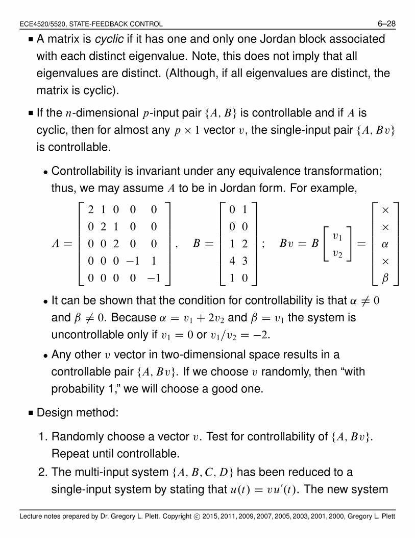
■ A matrix is cyclic if it has one and only one Jordan block associated
with each distinct eigenvalue. Note, this does not imply that all
eigenvalues are distinct. (Although, if all eigenvalues are distinct, the
matrix is cyclic).
■ If the n-dimensional p-input pair fA; Bg is controllable and if A is
cyclic, then for almost any p " 1 vector v, the single-input pair fA; Bvg
is controllable.
$ Controllability is invariant under any equivalence transformation;
thus, we may assume A to be in Jordan form. For example,
A D
2
6666664
2 1 0 0 0
0 2 1 0 0
0 0 2 0 0
0 0 0 !1 1
0 0 0 0 !1
3
7777775
; B D
2
6666664
0 1
0 0
1 2
4 3
1 0
3
7777775
I Bv D B
"
v1
v2
#
D
2
6666664
"
"
˛
"
ˇ
3
7777775
$ It can be shown that the condition for controllability is that ˛ ¤ 0
and ˇ ¤ 0. Because ˛ D v1 C 2v2 and ˇ D v1 the system is
uncontrollable only if v1 D 0 or v1=v2 D !2.
$ Any other v vector in two-dimensional space results in a
controllable pair fA; Bvg. If we choose v randomly, then “with
probability 1,” we will choose a good one.
■ Design method:
1. Randomly choose a vector v. Test for controllability of fA; Bvg.
Repeat until controllable.
2. The multi-input system fA; B; C; Dg has been reduced to a
single-input system by stating that u.t/ D vu0.t/. The new system
Lecture notes prepared by Dr. Gregory L. Plett. Copyright c# 2015, 2011, 2009, 2007, 2005, 2003, 2001, 2000, Gregory L. Plett
ECE4520/5520, STATE-FEEDBACK CONTROL 6–29
is fA; Bv; C; Dg with input u0.t/ and output y.t/. Use single-input
design methods such as Bass–Gura or Ackermann to find k to
place the poles of the single-input system. Then, the overall state
feedback is: u.t/ D vu0.t/ and u0.t/ D !kx.t/ so u.t/ D !vkx.t/.
Therefore, K D vk.
■ What if A is not cyclic? It can be shown that if fA; Bg is controllable
then for almost any p " n real constant matrix K1 the matrix .A ! BK1/
has only distinct eigenvalues, and is therefore cyclic. Randomly
choose K1 matrices until .A ! BK1/ is cyclic. Then, design for this
system.
■ Use small random numbers for low control effort.
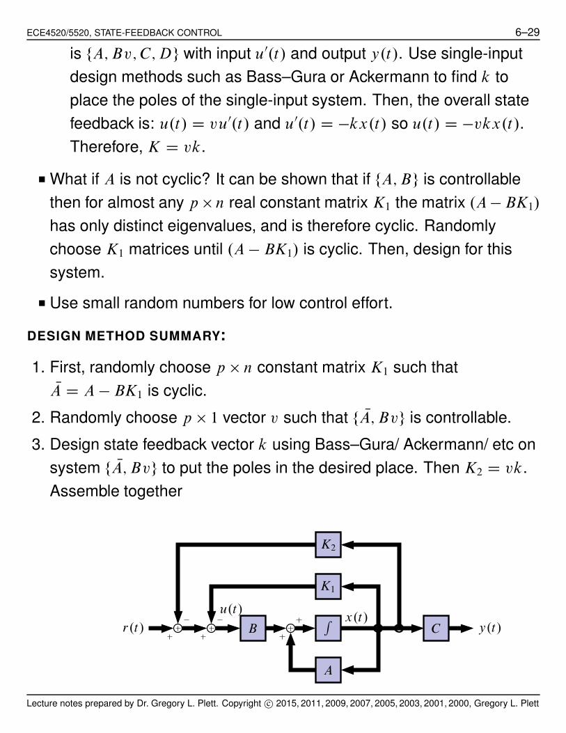
DESIGN METHOD SUMMARY:
1. First, randomly choose p " n constant matrix K1 such thatNA D A ! BK1 is cyclic.
2. Randomly choose p " 1 vector v such that f NA; Bvg is controllable.
3. Design state feedback vector k using Bass–Gura/ Ackermann/ etc on
system f NA; Bvg to put the poles in the desired place. Then K2 D vk.
Assemble together
K1
K2
A
B CR
r.t/ y.t/
u.t/x.t/
Lecture notes prepared by Dr. Gregory L. Plett. Copyright c# 2015, 2011, 2009, 2007, 2005, 2003, 2001, 2000, Gregory L. Plett
ECE4520/5520, STATE-FEEDBACK CONTROL 6–30
4. Design may be summed up as u.t/ D r.t/ ! .K1 C K2/x.t/.
Lyapunov-equation design
DESIGN METHOD:
1. Select an n " n matrix F with a set of desired eigenvalues that
contain no eigenvalues of A.
■ Make F real! If you have desired complex modes, use the real
modal form.
■ Don’t repeat eigenvalues in a diagonal matrix or fF; NKg will not be
observable. Use a Jordan form for repeated desired modes.
2. Randomly select p " n matrix NK such that fF; NKg is “observable.”
3. Solve for the unique T in the Lyapunov equation AT ! TF D B NK.
4. If T is singular, select a different NK and repeat. If T is nonsingular, we
compute K D NKT !1 and .A ! BK/ has the desired eigenvalues.
■ If T is nonsingular, the Lyapunov equation and KT D NK imply
.A ! BK/T D TF or A ! BK D TF T !1:
■ So, .A ! BK/ and F are similar and have same set of eigenvalues.
Where to from here?
■ In the design of state-feedback control, we assumed that all states of
our plant were measured.
■ This is often impossible to do or too expensive.
■ So, we now investigate methods of reconstructing the plant state
vector given only limited measurements.
Lecture notes prepared by Dr. Gregory L. Plett. Copyright c# 2015, 2011, 2009, 2007, 2005, 2003, 2001, 2000, Gregory L. Plett