StatCharrms Users Guide

2014-09-10

Written and Programmed By:

Joe Swintek, BTS

Based on StatCharrms SAS version developed by:

Dr. John Green, DuPont Applied Statistics Group, Stine-Haskell Research Center

Additional Testing By:

Kevin Flynn, USEPA

Jon Haselman, USEPA

Funded By:

USEPA under Contract EP-D-13-052

2 of 43

Table of Contents Introduction: ................................................................................................................................................. 2

Read Me: ....................................................................................................................................................... 2

Examples: ...................................................................................................................................................... 3

Histology Analysis (RSCABS): ......................................................................................................................... 4

Example Data and Format: ........................................................................................................................ 4

Specifying Identification Fields: ................................................................................................................ 4

Running RSCABS ........................................................................................................................................ 5

Time to Event Analysis: ................................................................................................................................. 7

Data Format: ............................................................................................................................................. 7

Data Specification: .................................................................................................................................... 7

Fecundity Analysis: ........................................................................................................................................ 8

Data Format: ............................................................................................................................................. 8

Data Specification: .................................................................................................................................... 9

Data Analysis: ......................................................................................................................................... 11

Analysis of Other End Points: ...................................................................................................................... 13

Data Format: ........................................................................................................................................... 13

Results ..................................................................................................................................................... 17

Flow Chart for Suggested Analysis .............................................................................................................. 19

Part 1: ...................................................................................................................................................... 19

Part 2: ...................................................................................................................................................... 19

3 of 43

Introduction: StatCharrms (Statistical analysis of Chemistry, Histopathology, and Reproduction endpoints using

Repeated measures and Multi-generation Studies) is a graphic user front end for ease of use in analyzing

data generated from the Medaka Extended One Generation Reproduction Test (MEOGRT) and Larval

Amphibian Gonad Development Assay (LAGDA). The analyses StatCharrms is capable of performing are;

Rao-Scott adjusted Cochran- Armitage test for trend By Slices (RSCABS), a Standard Cochran- Armitage

test for trend By Slices (SCABS), mixed effects cox proportional model, Jonckheere-Terpstra step down

trend test, Kruskal–Wallis, Dunn test, one way ANOVA, weighted ANOVA, mixed effects ANOVA, repeated

measures ANOVA, and Dunnett test.

Read Me: StatCharrms includes a read me button, pressing it will display the authors, references, and

change logs.

4 of 43

Examples: Before you start an analysis in StatCharrms you may want to use the provided examples module.

This module will generate all example data sets used in the StatCharrms user guide along with their

associated results.

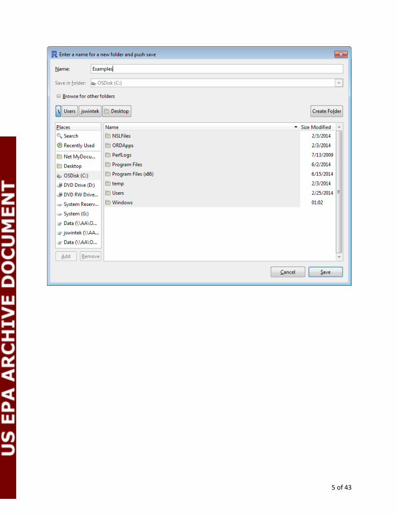
To run the examples just click on the Examples button from the main window. This will bring up

a dialog box. Within the box type the name of a new folder. This will create a new folder with the

example data sets and results.

5 of 43

6 of 43

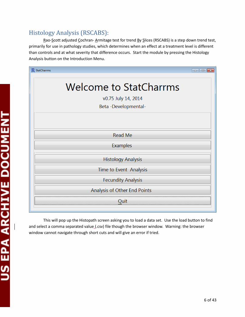
Histology Analysis (RSCABS): Rao-Scott adjusted Cochran- Armitage test for trend By Slices (RSCABS) is a step down trend test,

primarily for use in pathology studies, which determines when an effect at a treatment level is different

than controls and at what severity that difference occurs. Start the module by pressing the Histology

Analysis button on the Introduction Menu.

This will pop up the Histopath screen asking you to load a data set. Use the load button to find

and select a comma separated value (.csv) file though the browser window. Warning: the browser

window cannot navigate through short cuts and will give an error if tried.

7 of 43

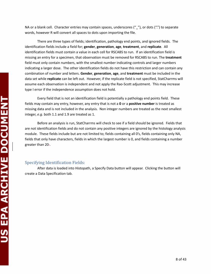
Example Data and Format: Below is the example histology data provided with StatCharrms.

Data sets must be in comma separated value (csv) format. Each column indicates a field and

each row indicates a specimen (a fish) with the exception of the first row which is the header row and

contains the names of the fields. As with any csv file imported into R, missing data is indicated by either

8 of 43

NA or a blank cell. Character entries may contain spaces, underscores (“_”), or dots (“.”) to separate

words, however R will convert all spaces to dots upon importing the file.

There are three types of fields; identification, pathology end points, and ignored fields. The

identification fields include a field for; gender, generation, age, treatment, and replicate. All

identification fields must contain a value in each cell for RSCABS to run. If an identification field is

missing an entry for a specimen, that observation must be removed for RSCABS to run. The treatment

field must only contain numbers, with the smallest number indicating controls and larger numbers

indicating a larger dose. The other identification fields do not have this restriction and can contain any

combination of number and letters. Gender, generation, age, and treatment must be included in the

data set while replicate can be left out. However, if the replicate field is not specified, StatCharrms will

assume each observation is independent and not apply the Rao-Scott adjustment. This may increase

type I error if the independence assumption does not hold.

Every field that is not an identification field is potentially a pathology end points field. These

fields may contain any entry, however, any entry that is not a 0 or a positive number is treated as

missing data and is not included in the analysis. Non integer numbers are treated as the next smallest

integer, e.g. both 1.1 and 1.9 are treated as 1.

Before an analysis is run, StatCharrms will check to see if a field should be ignored. Fields that

are not identification fields and do not contain any positive integers are ignored by the histology analysis

module. These fields include but are not limited to; fields containing all 0’s, fields containing only NA,

fields that only have characters, fields in which the largest number is 0, and fields containing a number

greater than 20 .

Specifying Identification Fields: After data is loaded into Histopath, a Specify Data button will appear. Clicking the button will

create a Data Specification tab.

9 of 43

10 of 43

All entries except for the “Replicate Variable” on the data specification tab must be specified. If

“Replicate Variable” is not specified StatCharrms will not apply the Rao-Scott adjustment which may

increase the type I error should study design indicate a replicate variable be needed. After all entry

forms are filled out, click on the “Confirm Selected Values and Variables” to set the selected variables

into StatCharrms. After the selection is set, you can navigate back to the main tab to perform RSCABS.

Note that at any time you may navigate back to the Data specification tab to change a selection, just re-

click the “Confirm Selected Values and Variables” to accept the change.

11 of 43

12 of 43

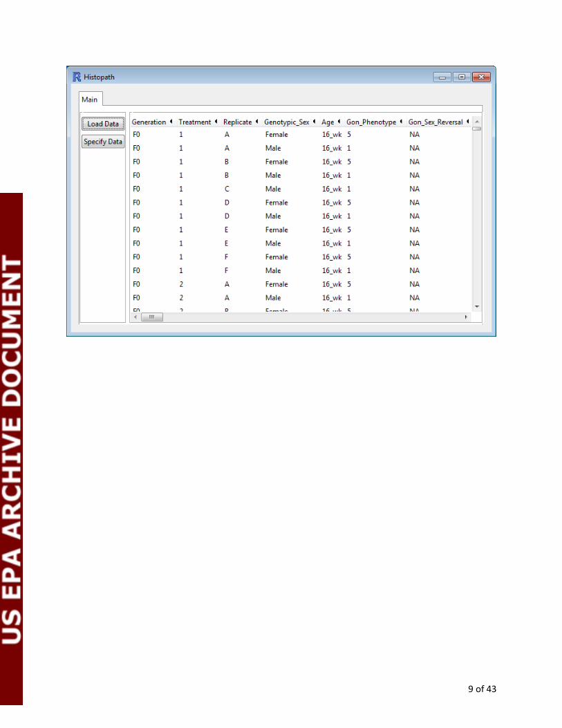
Running RSCABS After the data has been specified, two buttons, “Run RSCABS” and “Run Other Analyses” will

appear on the Histopath main tab. Pressing “Run RSCABS” will perform a Rao-Scott adjusted Cochran-

Armitage test for trend By Slices on the selected data.

13 of 43

After the data is run, you may save the result by using the “Save Result” button. Clicking the

“Run Other Analyses” button will pop up a window containing 4 buttons; “Run SCABS”, “Get Details on a

Response”, “Get Details on all Responses”, and “Save”.

14 of 43

The “Run SCABS” button will run the Standard Cochran- Armitage test for trend By Slices on the

selected data without the Rao-Scott adjustment. A table will appear with the results of the analysis. It

includes the name of the response (Response), the treatment level that was tested (Treatment), the

severity score (Rscore), a T-Value with corresponding p-value, and a column indicating significance at the

0.05 level.

15 of 43

The “Get Details on a Response” will supply three tables for selected response; a table for the

chi-squared (χ2) test for heterogeneity of between-replicate variances , a frequency table which contains

the total observations for each treatment-score combination, and finally, a table for the replication of

RSCABS for that treatment. The “Signif” column has three significance levels ‘*’, ‘**’, and ‘***’ for p-

values of 0.05, 0.01, and 0.001 respectively.

16 of 43

The Save button will save the current result displayed in the window.

Finally the “Get Details on all Responses” button will generate the three tables generated by the “Get

Details on a Response” for all responses. It does this by creating a new folder and populating that folder

with HTML files containing the information.

17 of 43

18 of 43

Time to Event Analysis: This module uses the coxme R package to perform Mixed Effect Cox Proportional Models. Start

by clicking on the “Time to Event Analysis” button.

19 of 43

Data Format: Start by loading a comma separated value (csv) file by using the “Load Data” button. Each

column indicates a field and each row, except the header row which contains the field names,

indicates an event for a single organism. As with any csv file imported into R, missing data is indicated

by either NA or a blank cell. Character entries many contain spaces, underscores (“_”), or dots (“.”)

to separate words, however R will convert all spaces to dots upon importing the file.

The fields needed for the time to event analysis are time, status, treatment, and replicate. All

entries in a field need to have a value in them. Any field containing NA or that is blank needs to be

removed from the data set before the analysis. Time can consist of either non-negative integers (called

numeric within the program) or dates. Status data must be either characters or numbers; StatCharrms

will convert censored events (such as death) to 0 and the event being tested for (such as a life stage) to

1. Treatment must be non-negative integers where the lowest number is the control and larger numbers

indicate higher treatment concentrations. Replicate can consist of either characters or numbers.

20 of 43

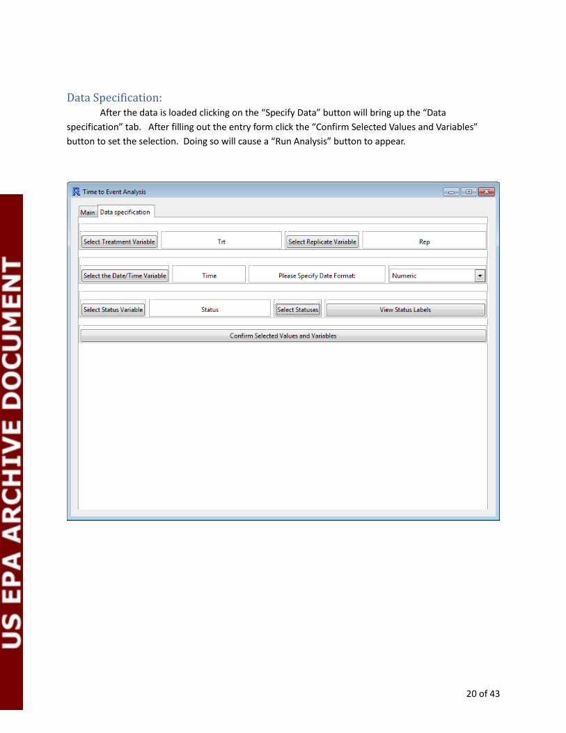
Data Specification: After the data is loaded clicking on the “Specify Data” button will bring up the “Data

specification” tab. After filling out the entry form click the “Confirm Selected Values and Variables”

button to set the selection. Doing so will cause a “Run Analysis” button to appear.

21 of 43

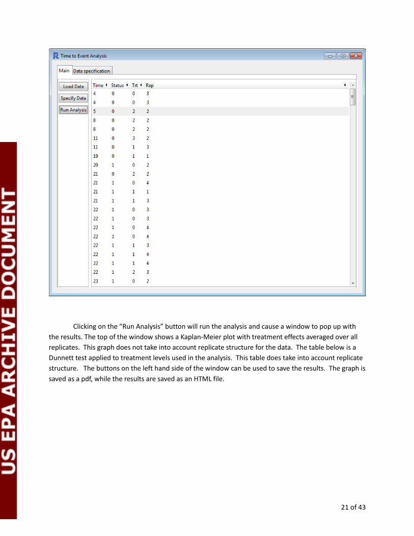
Clicking on the “Run Analysis” button will run the analysis and cause a window to pop up with

the results. The top of the window shows a Kaplan-Meier plot with treatment effects averaged over all

replicates. This graph does not take into account replicate structure for the data. The table below is a

Dunnett test applied to treatment levels used in the analysis. This table does take into account replicate

structure. The buttons on the left hand side of the window can be used to save the results. The graph is

saved as a pdf, while the results are saved as an HTML file.

22 of 43

23 of 43

Fecundity Analysis: The fecundity analysis is the suggested analysis for fecundity in the MEOGRT guidelines. The

analysis defaults to a one sided step down t-test on treatment using a one way ANOVA. The module is

also capable of calculating a repeated measures ANOVA using time and treatment as fixed effects and

replicate as a random effect.

Start the fecundity analysis by clicking on the “Fecundity Analysis” button from the main window.

Data Format: This will pop up a screen asking you to load a data set. Use the load button to find and select

a comma separated value file though the browser window. Each column in the file should indicate a

field and each row should indicate an observation for a pair on a given day, except the header row

which contains the field names. As with any csv file imported into R, missing data is indicated by

24 of 43

either NA or a blank cell. Character entries many contain spaces, underscores (“_”), or dots (“.”) to

separate words, however R will convert all spaces to dots upon importing the file.

The data set needs at least 3 fields; treatment, replicate, and a response. Time and generation

can be used in the analysis but are not strictly needed. The time, treatment, and replicate fields need to

have a value in them. Any of these fields containing NA or that are blank need to be removed from the

data set before the analysis. generation may have missing data, but any entry corresponding to the

missing data will be ignored in the analysis. The response field may also have missing data, however

every time-treatment combination needs at least one non-missing value in the response field in order

for StatCharrms to run. Time or time-treatment values without associated response values should be

removed from the data set prior to loading the data set into StatCharrms.

Time can consist of either non-negative integers (called numeric within the program) or

dates. Treatment needs to consist of non-negative integers where the lowest number is the control and

larger numbers indicate higher treatment concentrations. Replicate and generation can be either

characters or numbers. Finally, the response can be any real number.

25 of 43

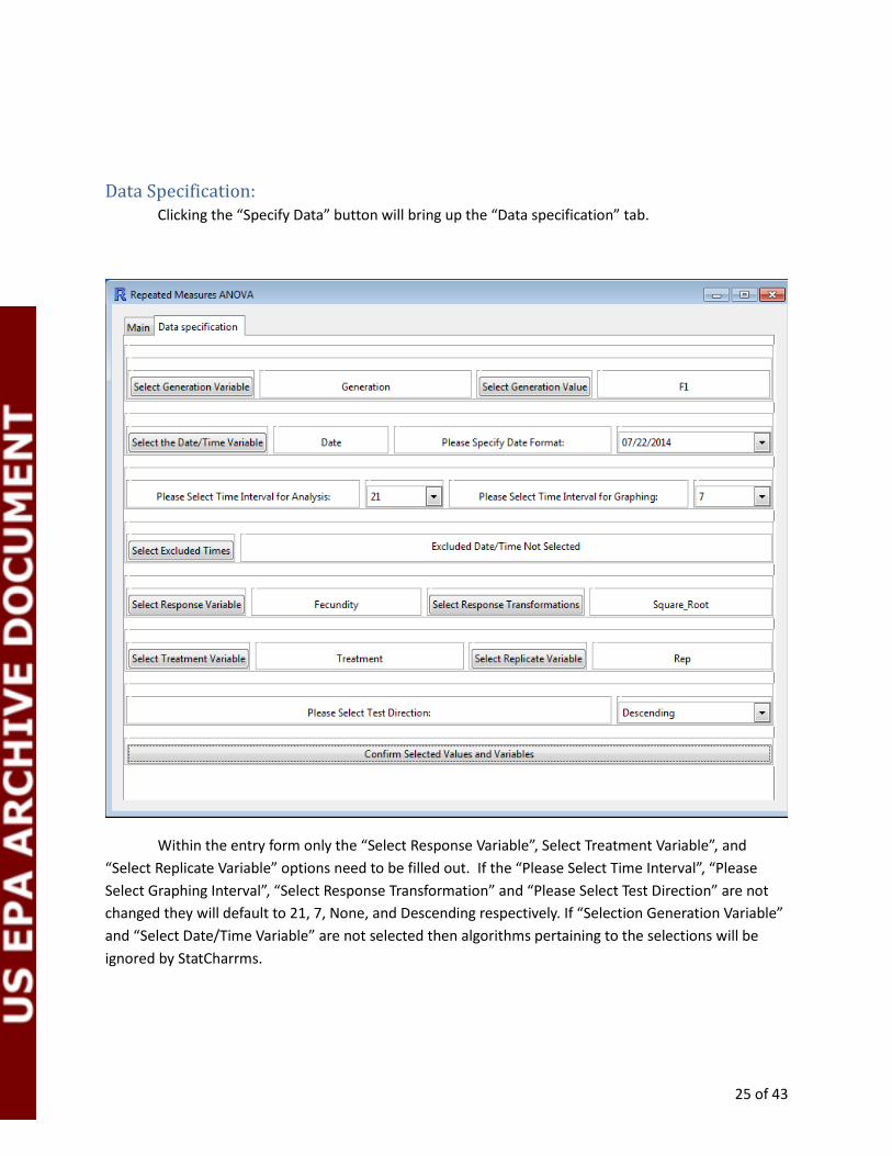
Data Specification: Clicking the “Specify Data” button will bring up the “Data specification” tab.

Within the entry form only the “Select Response Variable”, Select Treatment Variable”, and

“Select Replicate Variable” options need to be filled out. If the “Please Select Time Interval”, “Please

Select Graphing Interval”, “Select Response Transformation” and “Please Select Test Direction” are not

changed they will default to 21, 7, None, and Descending respectively. If “Selection Generation Variable”

and “Select Date/Time Variable” are not selected then algorithms pertaining to the selections will be

ignored by StatCharrms.

26 of 43

Each selection does the following:

Select Generation Variable:

This will select the name of the column the generation information is stored in. This selection is

optional and if generation is not used it may be left blank or explicitly selected as “Not Used”.

Select Generation Value:

If a generation variable is selected, this is used to select the generation StatCharrms will perform

the analysis on. StatCharrms performs an analysis of fecundity on only one generation at a time.

Select Date/Time Variable:

This will select the name of the column the time information is stored in. This selection is

optional and if time is not used it may be left blank or explicitly selected as “Not Used”.

Please Specify Date format:

This will display the current date in a variety of formats. The default is the ISO 6801

international standard (2001-12-31). Other formats are acceptable, including numbers (i.e.,1,2,3…). For

number dates, select “Numeric” at the bottom of the list. If StatCharrms does not recognize the date

format it will give a warning “Incompatible date format please reselect date format. “ If date format

does not work for some date, StatCharrms will inform you of the rows that do not work for that date

format and ask you to either change the date format or remove the rows. StatCharrms will not run

unless it recognizes the date format for all the rows of data.

Please Select Time Interval for Analysis:

This is the number of days the data will be averaged over for the analysis. Selecting a number

greater than or equal to the maximum number of days used in the analysis will cause StatCharrms to use

a one way ANOVA, while selecting less than maximum number of days used in the analysis will cause

StatCharrms to use a repeated measures ANOVA. It defaults to 21, the number of days specified in the

MEOGRT protocol.

Please Select Time Interval for Graphing:

This is the number of days the data will be averaged over for the graphs generated by

StatCharrms. It defaults to 7 days or a week.

27 of 43

Select Excluded Times:

This selects the dates or times that are to be excluded from the analysis. You may select

multiple dates by holding the shift or ctrl key when selecting in the selection window. If you do not wish

to exclude any date you may skip this entry or explicitly choose “Exclude None” in the exclusion window.

Select Response Variable:

This selects the name of the column that contains the response variable for the analysis . This is

a required entry.

Select Response Transformation:

This selects the transformation applied to the response variable. The selectable transformations

are; no transformation (None), Log (X), Log(X+1), square root(X) , arcsine(square root(X)) (‘Arcsine’) , and

a rank transformation. The rank transformation uses a Blom rank transformation on the response taking

the mean of any ties. If a value is not selected the analysis will default to using no transformation.

Select Treatment Variable:

This selects the name of the column that contains the treatment values for the analysis. This is a

required entry.

Select Replicate Variable:

This selects the name of the column that contains the replicate values for the analysis. This is a

required entry.

Please Select Test Direction:

This is the direction of the t test. Descending and ascending are one sided tests while, “both”

uses a two sided test. If not changed, StatCharrms will default to a descending test.

After the form is filled, clicking the “Confirm Selected Values and Variables” button will open up

the “Run Analysis” button in the “Main” tab. At any point you may navigate back to the “Data selection”

tab and change an entry. Just re-click the “Confirm Selected Values and Variables” button to accept the

change.

28 of 43

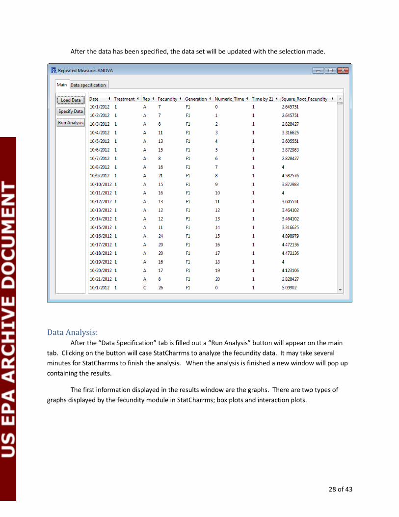
After the data has been specified, the data set will be updated with the selection made.

Data Analysis: After the “Data Specification” tab is filled out a “Run Analysis” button will appear on the main

tab. Clicking on the button will case StatCharrms to analyze the fecundity data. It may take several

minutes for StatCharrms to finish the analysis. When the analysis is finished a new window will pop up

containing the results.

The first information displayed in the results window are the graphs. There are two types of

graphs displayed by the fecundity module in StatCharrms; box plots and interaction plots.

29 of 43

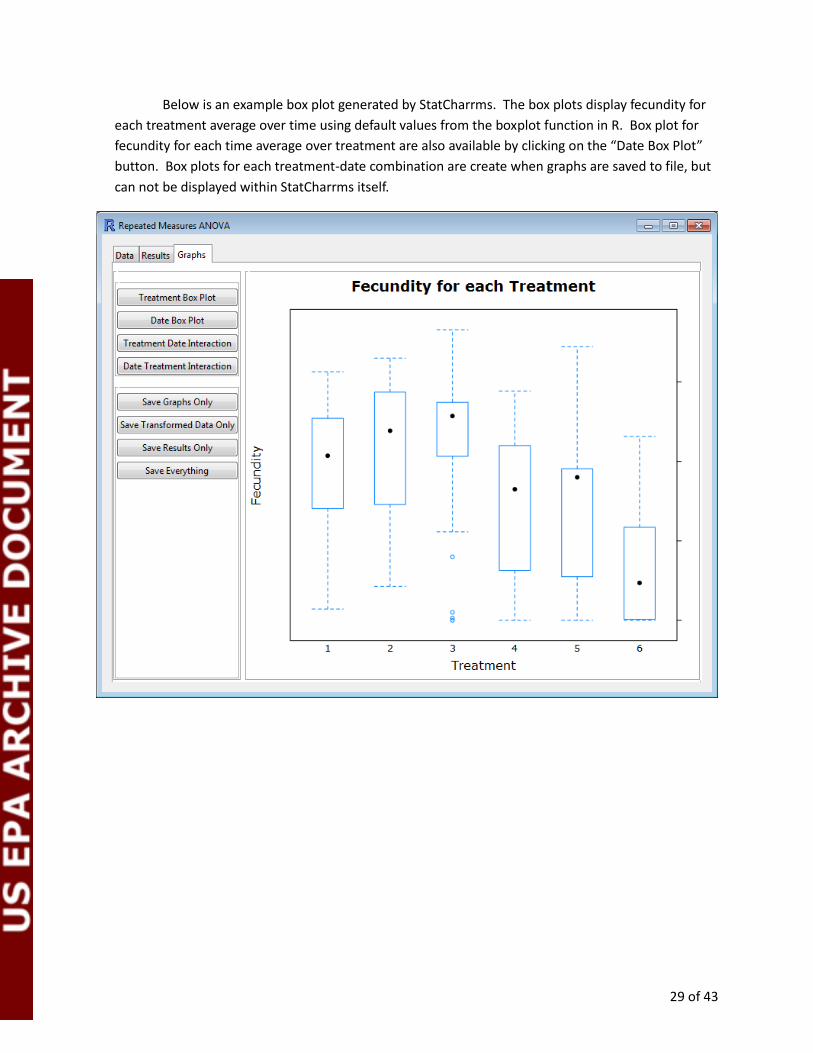
Below is an example box plot generated by StatCharrms. The box plots display fecundity for

each treatment average over time using default values from the boxplot function in R. Box plot for

fecundity for each time average over treatment are also available by clicking on the “Date Box Plot”

button. Box plots for each treatment-date combination are create when graphs are saved to file, but

can not be displayed within StatCharrms itself.

30 of 43

The second type of plots generated are Interaction plots. These plots show mean response for each

treatment –time combination. These plots are often used to assess interaction. If the lines for each

“Date” (the time variable used in the example analysis) cross there is a possibility of interaction between

time and treatment.

31 of 43

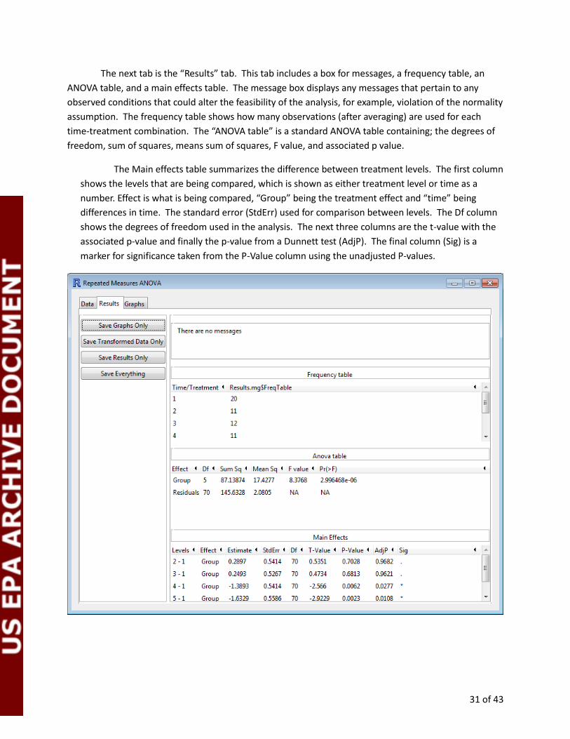
The next tab is the “Results” tab. This tab includes a box for messages, a frequency table, an

ANOVA table, and a main effects table. The message box displays any messages that pertain to any

observed conditions that could alter the feasibility of the analysis, for example, violation of the normality

assumption. The frequency table shows how many observations (after averaging) are used for each

time-treatment combination. The “ANOVA table” is a standard ANOVA table containing; the degrees of

freedom, sum of squares, means sum of squares, F value, and associated p value.

The Main effects table summarizes the difference between treatment levels. The first column

shows the levels that are being compared, which is shown as either treatment level or time as a

number. Effect is what is being compared, “Group” being the treatment effect and “time” being

differences in time. The standard error (StdErr) used for comparison between levels. The Df column

shows the degrees of freedom used in the analysis. The next three columns are the t-value with the

associated p-value and finally the p-value from a Dunnett test (AdjP). The final column (Sig) is a

marker for significance taken from the P-Value column using the unadjusted P-values.

32 of 43

The last tab shows the data used in the analysis after all adjustments.

33 of 43

Analysis of Other End Points:

The “Analysis of Other End Points” module implements one or more of the following tests;

Jonckheere-Terpstra step down trend test, Kruskal–Wallis, Dunn test, one way ANOVA, weighted ANOVA,

mixed effects ANOVA, and Dunnett test.

Start the module by clicking on the “Analysis of Other End Points” button

34 of 43

Data Format: Start by loading a comma separated value (csv) file by using the “Load Data” button. Each

column indicates a field and each row indicates a specimen, except the header row that contains the

names of the fields. As with any csv file imported into R, missing data is indicated by either NA or a

blank cell. Character entries many contain spaces, underscores (“_”), or dots (“.”) to separate words,

however R will convert all spaces to dots upon importing the file.

The only required information needed in the data set are a column for treatment and at least

one response that meets the requirements for a response. Optional information that can be used in the

analysis can be a column for age, replicate, ANOVA weights, gender, and generation. The acceptability

requirements of each column are listed below.

Treatment:

Treatment needs to contain only numbers. The lowest number needs to correspond to control

and each higher number need to correspond to higher doses. Rows without values for treatment need

to be removed before the data is loaded into StatCharrms.

Response:

A response must have; values in at least two treatments, the values must differ between

treatments, and contain only numbers. If a response is selected that has values in only one treatment or

the same values in different treatments, StatCharrms will warn you and remove the response from the

analysis. If a row does not have a number for a selected response, StatCharrms will warn you, remove

the row from the analysis of that response, then proceed with the analysis.

Replicate:

Replicate can contain characters and/or numbers. Rows containing missing values in the

replicate column of the data need to be removed prior to importing the data into StatCharrms.

ANOVA Weights:

ANOVA weights need to contain only numbers. Rows containing missing values in the ANOVA

weights column of the data need to be removed prior to importing the data into StatCharrms.

Age, Gender, and Generation:

The age, gender, and generation columns in the data set can contain any combination of

numbers and letters. Rows containing missing data in any of these columns are ignored by StatCharrms,

effectively removing the rows before the analysis.

35 of 43

Data Specification:

After a data set is imported into StatCharrms a “Specify Data” button will appear on the main

tab. Clicking on it will bring up the “Data specification” tab.

Within the entry form only the “Select Treatment Variable” and “Select Endpoints to Test” option need

to be filled out. If the “Select Transformation”, “Select Test Type”, and “Select Test Direction” are not

changed they will default to “none”, “Auto” and “Both” respectively. If “Select Generation Variable”,

“Select Dose Variable”, “Select Age Variable”, “Select Gender Variable”, or “Select Weights Variable” are

not selected, then algorithms pertaining to the selections will be ignored by StatCharrms.

Each selection does the follows:

36 of 43

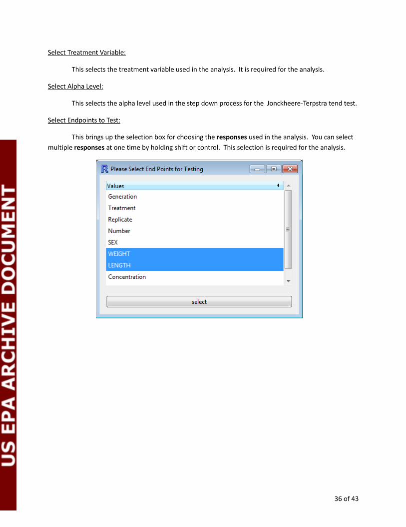
Select Treatment Variable:

This selects the treatment variable used in the analysis. It is required for the analysis.

Select Alpha Level:

This selects the alpha level used in the step down process for the Jonckheere-Terpstra tend test.

Select Endpoints to Test:

This brings up the selection box for choosing the responses used in the analysis. You can select

multiple responses at one time by holding shift or control. This selection is required for the analysis.

37 of 43

Select Test Type

This module of StatCharrms allows for different tests for significance. “Auto” follows the flow

listed at the end of the document. “Pairwise” performs both a Dunn and a Dunnett test on the data.

“Trend” performs the Jonckheere-Terpstra test for trend. “Force Non-Parametric” forces a Jonckheere-

Terpstra step down trend test, Kruskal–Wallis, and a Dunn test. Lastly “Force Tamhane-Dunnett” forces a

Tamhane-Dunnett test.

Select Test Direction:

This is the direction of the t test for significance. Increasing and Decreasing are one sided tests

while “both” uses a two sided test. If this values is not changed StatCharrms will use a two sided test.

Select Response Transformation:

This selects the transform applied to the response variable. The selectable transformation are;

no transformation (None), Log (X), Log(X+1), square root(X) , arcsine(square root(X)) (‘Arcsine’) , and a

rank transformation. The rank transformation uses a Blom rank transformation on the response taking

the mean of any ties. See the appendix for more details. If a value is not selected the analysis will

default to using no transformation.

38 of 43

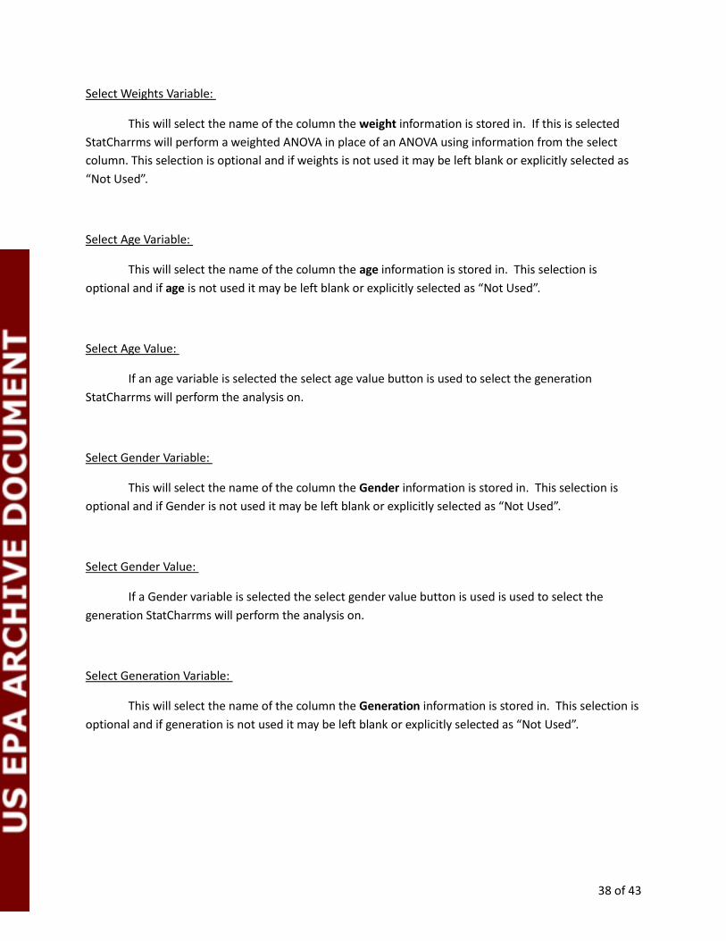
Select Weights Variable:

This will select the name of the column the weight information is stored in. If this is selected

StatCharrms will perform a weighted ANOVA in place of an ANOVA using information from the select

column. This selection is optional and if weights is not used it may be left blank or explicitly selected as

“Not Used”.

Select Age Variable:

This will select the name of the column the age information is stored in. This selection is

optional and if age is not used it may be left blank or explicitly selected as “Not Used”.

Select Age Value:

If an age variable is selected the select age value button is used to select the generation

StatCharrms will perform the analysis on.

Select Gender Variable:

This will select the name of the column the Gender information is stored in. This selection is

optional and if Gender is not used it may be left blank or explicitly selected as “Not Used”.

Select Gender Value:

If a Gender variable is selected the select gender value button is used is used to select the

generation StatCharrms will perform the analysis on.

Select Generation Variable:

This will select the name of the column the Generation information is stored in. This selection is

optional and if generation is not used it may be left blank or explicitly selected as “Not Used”.

39 of 43

Select Generation Value:

If a generation variable is selected the select generation value button is used to select the

generation StatCharrms will perform the analysis on. StatCharrms performs an analysis of fecundity

on one generation at a time.

After the form is filled clicking the “Confirm Selected Values and Variables” button will open up the

“Run Analysis” button in the “Main” tab. At any point you may navigate back to the “Data specification”

tab and change an entry. Just re-click the “Confirm Selected Values and Variables” button to accept the

change.

40 of 43

Results

Pressing the “Run Analysis” button will cause StatCharrms to perform the analysis on the selected

endpoints. This will pop up a window containing a tab for graphs and a tab for the analysis of each

tested endpoint.

41 of 43

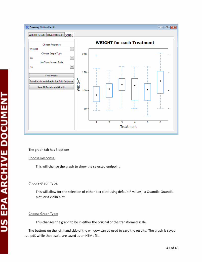
The graph tab has 3 options

Choose Response:

This will change the graph to show the selected endpoint.

Choose Graph Type:

This will allow for the selection of either box plot (using default R values), a Quantile-Quantile

plot, or a violin plot.

Choose Graph Type:

This changes the graph to be in either the original or the transformed scale.

The buttons on the left hand side of the window can be used to save the results. The graph is saved

as a pdf, while the results are saved as an HTML file.

42 of 43

Each of the results tab will results tabs will contain a summary table. In addition to the summary table it

will contain tables pertaining to the selected analysis. In this case the results tab contains a table for the

test for monotonicity and a table for the Jonckheere-Terpstra test for trend. If other analyses (Dunnett

for example) are run, the results tab will include tables pertaining to those results.

43 of 43

Flow Chart for Suggested Analysis

Part 1:

44 of 43

Part 2: