1

Stata Program Notes Biostatistics: A Guide to Design, Analysis, and Discovery Chapter 9: Nonparametric Tests Program Notes Outline Note 9.1 – The Sign Test and Wilcoxon Signed Rank Test Note 9.2 – The Wilcoxon Rank Sum Test or Mann-Whitney test Note 9.3 – The Kruskal-Wallis Test Note 9.4 – The Friedman Test

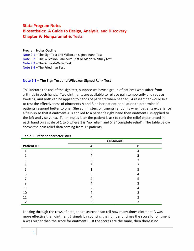
Note 9.1 – The Sign Test and Wilcoxon Signed Rank Test To illustrate the use of the sign test, suppose we have a group of patients who suffer from arthritis in both hands. Two ointments are available to relieve pain temporarily and reduce swelling, and both can be applied to hands of patients when needed. A researcher would like to test the effectiveness of ointments A and B on her patient population to determine if patients respond better to one. She administers ointments randomly when patients experience a flair-up so that if ointment A is applied to a patient’s right hand then ointment B is applied to the left and vise-versa. Ten minutes later the patient is ask to rank the relief experienced in each hand on a scale of 1 to 5 where 1 is “no relief” and 5 is “complete relief”. The table below shows the pain relief data coming from 12 patients.

Table 1. Patient characteristics

Ointment

Patient ID A B

1 2 4 2 4 5 3 3 3 4 3 2 5 1 5 6 3 4 7 4 5 8 4 3 9 2 4 10 2 3 11 4 2 12 3 3

Looking through the rows of data, the researcher can tell how many times ointment A was more effective than ointment B simply by counting the number of times the score for ointment A was higher than the score for ointment B. If the scores are the same, then there is no

2

noticeable difference between the two ointments. The actual score differences between ointment A and B are provided below:

(ointment A – ointment B): -2, -1, 0, +1, -4, -1, -1, +1, -2, -1, +2, 0 The null hypothesis of no difference between ointments A and B is represented by Δ = 0. The researcher can write the null and alternative hypotheses using the following notation: H0: Δ = 0 versus Ha: Δ ≠ 0. To use the sign test, consider the signs of the differences shown below. Notice that differences equal to 0 were eliminated because a positive or negative sign cannot be assigned to 0. The data look as follows:

(ointment A – ointment B): -, -, eliminated, +, -, -, -, +, -, -, +, eliminated. Out of the 10 signs, one would expect 5 to be positive and 5 to be negative. We could also say that we expect 50%, 1/2, or 0.5 of the signs to be positive, then the following null and alternative hypotheses would apply: H0: π = 0.5 versus Ha: π ≠ 0.5 Under the null hypothesis, the expected number of positive signs is np or (10/2) where n is the number on nonzero observations. The variance is np(1-p) or (10/4). In both cases, 1/2 was substituted for p, and 10 was substituted for n. If the normal approximation to the binomial distribution is to be used, we can form a test statistic that follows a standard normal distribution, where S is the number of positive signs observed:

. Given the number of positive signs observed is 3 = S, the number expected is 5 = 10/2 = np, and the standard deviation is the square root of 10/4 = sqrt(10/4) = sqrt(5/2); therefore,

.

4n

npSz

26.1

25

2

410

53

z

3

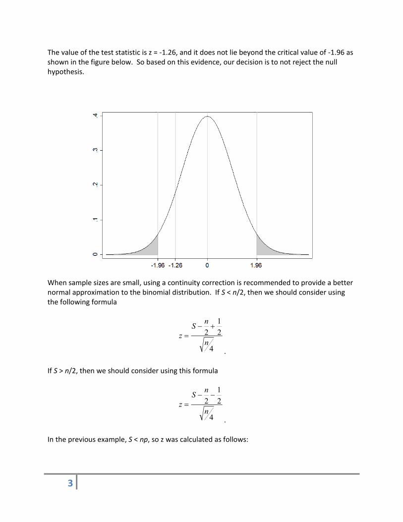
The value of the test statistic is z = -1.26, and it does not lie beyond the critical value of -1.96 as shown in the figure below. So based on this evidence, our decision is to not reject the null hypothesis.

When sample sizes are small, using a continuity correction is recommended to provide a better normal approximation to the binomial distribution. If S < n/2, then we should consider using the following formula

. If S > n/2, then we should consider using this formula

. In the previous example, S < np, so z was calculated as follows:

4

2

1

2

n

nS

z

4

2

1

2

n

nS

z

4

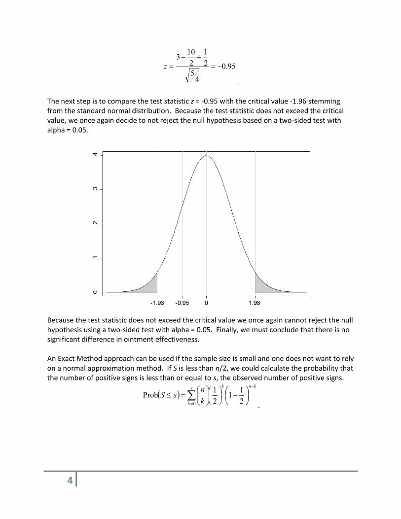
. The next step is to compare the test statistic z = -0.95 with the critical value -1.96 stemming from the standard normal distribution. Because the test statistic does not exceed the critical value, we once again decide to not reject the null hypothesis based on a two-sided test with alpha = 0.05.

Because the test statistic does not exceed the critical value we once again cannot reject the null hypothesis using a two-sided test with alpha = 0.05. Finally, we must conclude that there is no significant difference in ointment effectiveness. An Exact Method approach can be used if the sample size is small and one does not want to rely on a normal approximation method. If S is less than n/2, we could calculate the probability that the number of positive signs is less than or equal to s, the observed number of positive signs.

.

95.0

45

2

1

2

103

z

knks

k k

nsS

2

11

2

1Prob

0

5

For our specific case the formula would look like the following:

The following Stata commands can be used to perform the calculations to find the probabilities for a binomial distribution with parameters n = 10 and π = 0.50. Notice that the Stata command comb(n,k) returns the combinatorial “n choose k”. Stata commands:

input s

0

1

2

3

4

5

6

7

8

9

10

end

gen prob = comb(10,s)*(0.5)^s*(1-0.5)^(10-s)

gen cumprob = sum(prob)

list

172.02

11

2

1

3

10

2

11

2

1

2

10

2

11

2

1

1

10

2

11

2

1

0

10

2

11

2

1103Prob

3103210211010100103

0

kk

k kS

6

The Stata output is provided below. Stata output:

+--------------------------+

| s prob cumprob |

|--------------------------|

1. | 0 .0009766 .0009766 |

2. | 1 .0097656 .0107422 |

3. | 2 .0439453 .0546875 |

4. | 3 .1171875 .171875 |

5. | 4 .2050781 .3769531 |

|--------------------------|

6. | 5 .2460938 .6230469 |

7. | 6 .2050781 .828125 |

8. | 7 .1171875 .9453125 |

9. | 8 .0439453 .9892578 |

10. | 9 .0097656 .9990234 |

|--------------------------|

11. | 10 .0009766 1 |

+--------------------------+

Notice that the probability mass function for the binomial distribution is symmetric about s = 5. Therefore, Prob(S ≤ 3) = Prob(S ≥ 7) = 0.172. Stata commands:

input oint_a oint_b

2 4

4 5

3 3

3 2

1 5

3 4

4 5

4 3

2 4

2 3

4 2

3 3

end

gen diff = oint_a - oint_b

signtest diff=0

With the Stata output below, note that for a two-tailed test, the p-value needs to be multiplied by 2 to obtain: 2*0.172 = 0.344. This value is shown on the last line of the Stata output below. Stata output:

Sign test

sign | observed expected

-------------+------------------------

positive | 3 5

negative | 7 5

zero | 2 2

-------------+------------------------

7

all | 12 12

One-sided tests:

Ho: median of diff = 0 vs.

Ha: median of diff > 0

Pr(#positive >= 3) =

Binomial(n = 10, x >= 3, p = 0.5) = 0.9453

Ho: median of diff = 0 vs.

Ha: median of diff < 0

Pr(#negative >= 7) =

Binomial(n = 10, x >= 7, p = 0.5) = 0.1719

Two-sided test:

Ho: median of diff = 0 vs.

Ha: median of diff != 0

Pr(#positive >= 7 or #negative >= 7) =

min(1, 2*Binomial(n = 10, x >= 7, p = 0.5)) = 0.3438

In another example, consider the data shown in Table 9.2 (in the textbook). The data provide day 1 and 2 caloric intake for the 14 boys who had the more extreme caloric intakes on day1. We would like to test for “reversion towards the mean”. Using the Stata commands below, the data can be brought in directly creating the dataset of interest. The variable day1 represents the day1 caloric intake, the variable day2 represents the day2 caloric, and the variable group distinguishes between the seven lowest values and the seven highest values. Stata commands:

input day1 day2 group

1053 2484 0

1292 810 0

1505 1925 0

1645 2269 0

1723 3163 0

1753 1054 0

1781 1844 0

2773 3236 1

2842 2849 1

3049 2573 1

3076 2431 1

3277 2185 1

3532 3289 1

4322 2926 1

end

For the seven lowest values, if the difference between day2 and day1 (day2 – day1) is positive, then the change was in the direction of the mean. For the seven highest values, if the difference between day1 and day2 (day1 – day2) is positive, then the change was in the direction of the mean. Calculate the variable diff as indicated below. Stata commands:

gen diff = day2 - day1 if group == 0

replace diff = day1 - day2 if group == 1

8

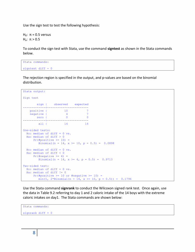
Use the sign test to test the following hypothesis: H0: π = 0.5 versus Ha: π > 0.5 To conduct the sign test with Stata, use the command signtest as shown in the Stata commands below. Stata commands:

signtest diff = 0

The rejection region is specified in the output, and p-values are based on the binomial distribution. Stata output:

Sign test

sign | observed expected

-------------+------------------------

positive | 10 7

negative | 4 7

zero | 0 0

-------------+------------------------

all | 14 14

One-sided tests:

Ho: median of diff = 0 vs.

Ha: median of diff > 0

Pr(#positive >= 10) =

Binomial(n = 14, x >= 10, p = 0.5) = 0.0898

Ho: median of diff = 0 vs.

Ha: median of diff < 0

Pr(#negative >= 4) =

Binomial(n = 14, x >= 4, p = 0.5) = 0.9713

Two-sided test:

Ho: median of diff = 0 vs.

Ha: median of diff != 0

Pr(#positive >= 10 or #negative >= 10) =

min(1, 2*Binomial(n = 14, x >= 10, p = 0.5)) = 0.1796

Use the Stata command signrank to conduct the Wilcoxon signed rank test. Once again, use the data in Table 9.2 referring to day 1 and 2 caloric intake of the 14 boys with the extreme caloric intakes on day1. The Stata commands are shown below: Stata commands:

signrank diff = 0

9

Stata output:

Wilcoxon signed-rank test

sign | obs sum ranks expected

-------------+---------------------------------

positive | 10 82 52.5

negative | 4 23 52.5

zero | 0 0 0

-------------+---------------------------------

all | 14 105 105

unadjusted variance 253.75

adjustment for ties 0.00

adjustment for zeros 0.00

----------

adjusted variance 253.75

Ho: diff = 0

z = 1.852

Prob > |z| = 0.0640

10

Note 9.2 – The Wilcoxon Rank Sum Test or Mann-Whitney test In Example 9.5 of the textbook, we apply the Wilcoxon rank sum test to the data presented in Table 9.5 on the proportion of calories from fat for boys in grades 5-6 and 7-8. The Stata command ranksum with the option by is used to perform this test as shown in the Stata commands below. The variable grade, in parentheses following the by option, is used to differentiate between the grade 5-6 values and the grade 7-8 values. Stata commands:

ranksum prop_from_fat, by(grade)

Stata output:

Two-sample Wilcoxon rank-sum (Mann-Whitney) test

group | obs rank sum expected

-------------+---------------------------------

0 | 19 336.5 323

1 | 14 224.5 238

-------------+---------------------------------

combined | 33 561 561

unadjusted variance 753.67

adjustment for ties -0.13

----------

adjusted variance 753.54

Ho: prop_f~t(group==0) = prop_f~t(group==1)

z = 0.492

Prob > |z| = 0.6229

11

Note 9.3 – The Kruskal-Wallis Test The Stata command kwallis using the by option was used to conduct the Kruskal-Wallis test. For example, use the data in Table 9.8 on simulated reductions in diastolic blood pressure for three treatment groups. Then use Stata commands below to conduct the analysis: Stata commands:

kwallis reduction, by(group)

Stata output:

Test: Equality of populations (Kruskal-Wallis test)

+------------------------+

| group | Obs | Rank Sum |

|-------+-----+----------|

| 0 | 8 | 164.50 |

| 1 | 15 | 436.50 |

| 2 | 16 | 179.00 |

+------------------------+

chi-squared = 19.133 with 2 d.f.

probability = 0.0001

chi-squared with ties = 19.207 with 2 d.f.

probability = 0.0001

12

Note 9.4 – The Friedman Test The Stata command friedman is used to conduct Friedman’s Test. The output also provides Kendall’s coefficient of concordance, and a single p-value is provided corresponding to both tests. If Stata version 9 does not contain the software update for friedman, you can install it using Stata’s internet resources.