Stat 591: Advanced Design of Experiments Rutgers ...
123
Stat 591: Advanced Design of Experiments Rutgers University Fall 2001 Steve Buyske
Transcript of Stat 591: Advanced Design of Experiments Rutgers ...

Stat 591: Advanced Design of ExperimentsRutgers University
Fall 2001
Steve Buyske

c©Steven Buyske and Richard Trout.

Contents
Lecture 1. Strategy of Experimentation I 11. Introduction 12. Stategy of Experimentation 13. Two Level Factorial Experiments 1
Lecture 2. Strategy of Experimentation II 151. Blocking 152. Fractional Factorial Designs 20
Lecture 3. Strategy of Experimentation III 291. Design Resolution 29
Lecture 4. Strategy of Experimentation IV 391. Fractional Factorials Continued 392. Screening Designs 40
Lecture 5. Response Surface Methodology I 471. Introduction 472. First order models 48
Lecture 6. Response Surface Methodology II 551. Steepest Ascent 552. Second Order Models 56
Lecture 7. Response Surface Methodology III 671. Canonical Form of Response Surface Models 672. Blocking in Response Surface Designs 71
Lecture 8. Response Surface Methodology IV 751. Bias and Variance 752. Practical Summary 783. EVOP 79
Lecture 9. Mixture Designs 811. Design and Analysis of Mixture Experiments 81
Lecture 10. Robust Design and Taguchi Methods 891. Robust Design ala Taguchi 892. Improving Robust Design from a statistical point of view 93
iii

iv CONTENTS
Lecture 11. Optimal Design 95
Lecture 12. Computer Experiments 1031. The Bayesian Approach 1042. The frequentist approach 105
Lecture 13. Gene Expression Arrays 1071. Introduction 1072. Designs 1073. Model 108
Lecture 14. Miscellany 1091. Errors in design parameters 1092. Split Plots 1103. Qualitative factors 1124. Incomplete Block Designs 1145. Balanced Incomplete Block Designs 1146. Partially Balanced Incomplete Block (PBIB) 117

LECTURE 1
Strategy of Experimentation I
“Experiments are an efficient way to learn about the world.”A. C. Atkinson
1. Introduction
• Text: Myers and Montgomery• Computer: SAS• Paper: oral presentation and short paper• Take Home Final: Simulation• Topics:
1. Strategy of Experimentation(a) 2-level factorial and fractional factorial(b) Screening experiments(c) Response surface methodology
2. Evolutionary Operation (EVOP)3. Optimal Design4. Computer-assisted design5. Mixture Experimentation6. Taguchi methods
2. Stategy of Experimentation
Typically, an experimenter is faced with a shopping list of factors, and mustdecide which ones are important. We would like to
1. Identify the primary factors.2. Identify the region of interest for the primary factors.3. Develop useful models in the region of the optimum settings of the factors.4. Confirm the results.
3. Two Level Factorial Experiments
Perhaps the most common experimental technique, to the horror of statisti-cians, is to vary one factor at a time. For example, an experimenter might hold allfactors fixed except for factor A, find the value for that factor that maximizes theresponse, and then repeat the process for factor B, and so on. We will see later whythis is not a good plan.
c©Steven Buyske and Richard Trout.
1

2 1. STRATEGY OF EXPERIMENTATION I
Recall that a factorial experiment considers all possible treatments consistingof combinations of factors. For example if there are two factors with four and threelevels, respectively, the experiment will have a total of 4 × 3 = 12 treatments.
In a two level factorial experiment, each factor is examined at two levels. Thesedesigns allow the examination of a relatively large number of factors with relativelyfew experimental runs. Why two levels? We need at least two to estimate the sizeof the effect, but using just two conserves resources.
They are restricted in terms of the size of the design space that can be explored.They can be modified to reduce the number of the runs as well as increase the
size of the design space.They are excellent building blocks.Three principles underlie our methods here. They are
Hierarchical Ordering Principle: Lower order effects are more likely to beimportant than higher order effects.
Effect Sparsity, or Pareto, Principle: The number of important effects is gen-erally small.
Effect Heredity Principle: For an interaction effect to be significant, (at leastone of) its parent effects should be significant.
You can find a fuller description in C. F. J. Wu & M. Hamada, Experiments: Plan-ning, Analysis, and Parameter Design Optimization, New York: John Wiley &Sons, Inc, 2000.

3. TWO LEVEL FACTORIAL EXPERIMENTS 3
22
B
A
23
B
A
C
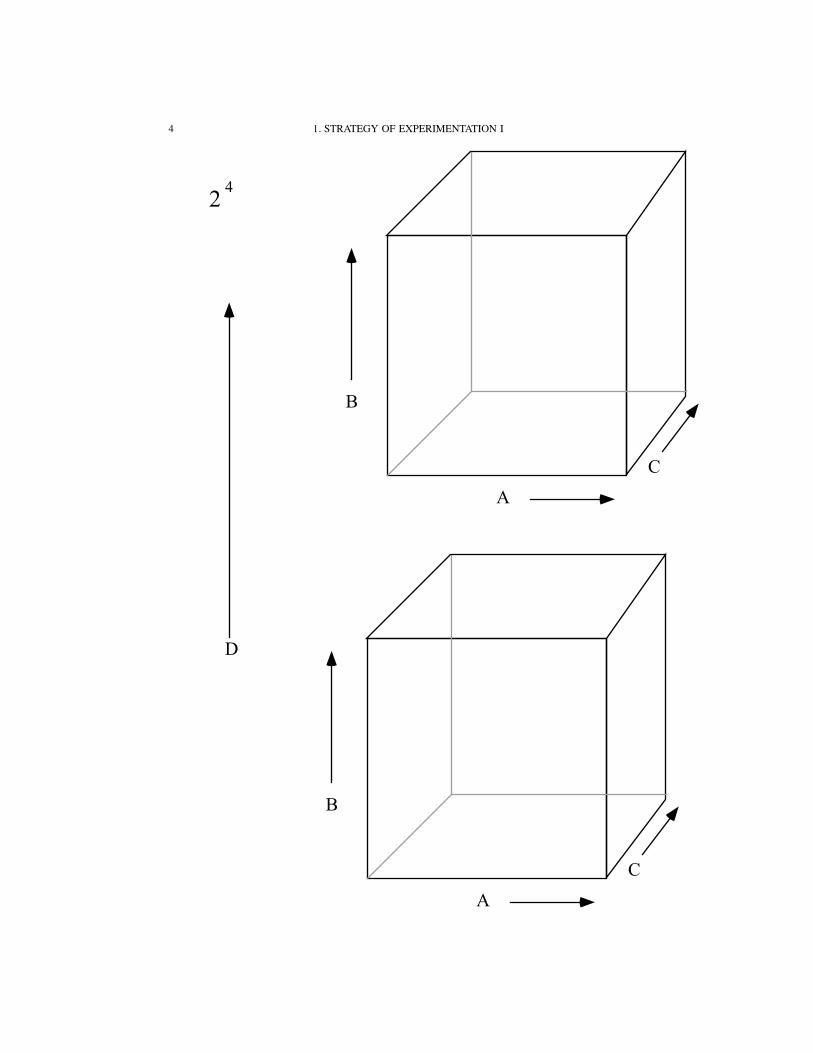
4 1. STRATEGY OF EXPERIMENTATION I
24
B
A
C
B
A
C
D

3. TWO LEVEL FACTORIAL EXPERIMENTS 5
Let us examine a two-factor factorial so that we can set up some basic notationas well as introduce some fundamental ideas.
Notationally the designs are 2K , where
K = number of factors,
and
2K = number of treatment combination runs (usually just called “treatments”).
For example if K = 2, the design requires 22 = 4 runs.
Run A B1 - -2 + -3 - +4 + +
B
(–,–) (+,–)
(–,+) (+,+)
A
We may also denote these points using the Yates notation:
Run Yates notation A B data1 (1) - - 22 a + - 43 b - + 64 ab + + 10
If we wanted to know the effect of variable A we could fix B, say −, and lookat the difference between A+ and A−, i.e., 4 − 2 = 2. We could then average thisvalue with the difference when B is high, 10 − 6 = 4. Therefore the A effect is
(4 − 2) + (10 − 6)
2= 2 + 4
2= 3,

6 1. STRATEGY OF EXPERIMENTATION I
or, using the Yates notation,
(a − (1)) + (ab − b)
2.
In general, we can determine how the effects are computed by constructing thefollowing table:
A B AB(1) - - +a + - -b - + -ab + + +
Therefore, except for the divisor,Mean = 1 + a + b + ab
A effect = −(1) + a − b + abB effect = −(1) − a + b + ab
AB effect = (1) − a − b + abFrom the effects we can generate the SS for each factor (recall that the sum of
squares for any contrast is the contrast squared divided by the number of observa-tions times the sum of the squares of the contrast coefficients).
SS = (numerator of effect)2
2K.
Therefore,
SSA = 62
4= 9
SSB = 102
4= 25
SSAB = 22
4= 1
SST OT = 35.
ANOVASource df SS MSTotal 3 35
A 1 9 9B 1 25 25
AB 1 1 1

3. TWO LEVEL FACTORIAL EXPERIMENTS 7
An alternative method to compute the effects and SS is to use the Yates Algo-rithm.
Order the data in the Yates standard notation.
Yates notation data col 1 col 2 effect= col K2K−1 SS= (col K)2
2K
(1) y1 y1 + ya y1 + ya + yb + yab
a ya yb + yab ya − y1 + yab − yb
b yb ya − y1 yb + yab − y1 − ya
ab yab yab − yb yab − yb − ya + y1
For the dataYates notation data col 1 col 2 effect= col K
2K−1 SS= (col K)2
2K
(1) 2 2 + 4 = 6 6 + 16 = 22 = ∑y 22/4 = 5.5 = ¯y 121=C.F.
a 4 6 + 10 = 16 2 + 4 = 6 3 9b 6 4 − 2 = 2 16 − 6 = 10 5 25ab 10 10 − 6 = 4 4 − 2 = 2 1 1
NB In the (1) row and the effect column, by dividing by 2K instead of 2K−1,we get the overall mean ¯y.
NB Because we have used -1 and +1 as the levels in our model, if you use aregression method to find the factor effects the coefficients you find will be one-halfof that given here.
The Yates Algorithm is also described in Appendix 10A of Box, Hunter, andHunter (on reserve).
Now let us consider a 23 factorial experiment given in Box, Hunter, and Hunter’sStatistics for Experimenters.
We have two factors, Temperature and Concentration, that are quantitative, andCatalyst which is qualitative. The response is the chemical yield.
Temperature Concentration Catalyst YieldT (– 160, + 180) C (–20, + 40) K (– A, +B) data
(1) – – – 60t + – – 72c – + – 54tc + + – 68k – – + 52tk + – + 83ck – + + 45tck + + + 80
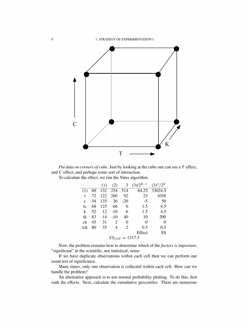
8 1. STRATEGY OF EXPERIMENTATION I
C
T
K
Put data on corners of cube. Just by looking at the cube one can see a T effect,and C effect, and perhaps some sort of interaction.
To calculate the effect, we run the Yates algorithm.
(1) (2) 3 (3)/2K−1 (3)2/2K
(1) 60 132 254 514 64.25 33024.5t 72 122 260 92 23 1058c 54 135 26 -20 -5 50tc 68 125 66 6 1.5 4.5k 52 12 -10 6 1.5 4.5tk 83 14 -10 40 10 200ck 45 31 2 0 0 0tck 80 35 4 2 0.5 0.5
Effect SSSST OT = 1317.5
Now, the problem remains how to determine which of the factors is important,“significant” in the scientific, not statistical, sense.
If we have duplicate observations within each cell then we can perform ourusual test of significance.
Many times, only one observation is collected within each cell. How can wehandle the problem?
An alternative approach is to use normal probability plotting. To do this, firstrank the effects. Next, calculate the cumulative percentiles. There are numerous

3. TWO LEVEL FACTORIAL EXPERIMENTS 9
was to do this. The first column below is probably best, but the second and thirdare easier if you are doing it by hand or calculator. The conclusions that you drawwill not be noticeably different.
Cum Percenti−3/8
# of effects+1/4 × 100 i−1/2# of effects × 100 i
# of effects × 100 Effect Source8.6 7.1 12.5 -5 C
22.4 21.4 25.0 0 CK36.2 35.7 37.5 0.5 TCK56.9 50.0 56.25 1.5 TC56.9 64.3 56.25 1.5 K77.6 78.6 75.0 10 TK91.4 92.9 87.5 23 T
NB The second column contains the values used in plotting on the next page.
Discuss Plotting this info on normal probability paper.

10 1. STRATEGY OF EXPERIMENTATION I
The problem with this approach is that you need to look at both tails of thedistribution as the sign of the effect is arbitrary as far as the importance of theeffect is concerned. People tend to miss important effects this way.
An alternative approach is to use half-normal probability plotting. This papercan be purchased for varying values of p or it can be constructed from the usualnormal probability paper. To do this, delete the scale for values of p less than 50%.For p greater than 50%, replace each value of P with P ′, where P ′ = 2P − 100.Now rank the absolute value of the effects and plot the data as was done earlier.People tend to see too many important effects this way.
Cum. Percent |Effect| Source7.1 0 CK
21.4 0.5 TCK35.7 1.5 TC50.0 1.5 K64.3 5 C78.6 10 TK92.9 23 T
See graph below.

3. TWO LEVEL FACTORIAL EXPERIMENTS 11
/*SAS code for ademonstration of normal and half normalprobability plots of effects fromfactorial experiments.Stat 591, Rutgers UniversitySteve Buyske Sept 99
*/
data effects;input effect @@;label effect=’Effect Size’;heffect=abs(effect);label heffect=’Abs Effect Size’;cards;23 -5 1.5 1.5 10 0 .5;;
run;
/* calculate normal scores */proc rank data=effects normal=blom out=normals;
/* normal=blom means use (i-3/8)/(# of effects +1/4)*/var effect;ranks neffect;
run;
data normals;set normals;label neffect=’Normal score’;run;
/* produce normal probability plot *//* the lines commented out below give low-res plots *//*proc plot nolegend data=normals;
title ’Normal Probability Plot’;plot effect*neffect=’*’ ;
run;*/
goptions ftext=none htext=1 cell;
proc gplot data=normals;

12 1. STRATEGY OF EXPERIMENTATION I
title ’Normal Probability Plot’;plot effect*neffect=effect;
run;
/* calculate half normal scores */proc rank data=effects out=hnranks;
var heffect;ranks hneffect;
run;
data hnormals;set hnranks nobs=n;label hneffect=’Half Normal score’;hneffect=probit(((hneffect-1/3)/(n+1/3))/2+.5);run;
/* produce half normal probability plot */
/*proc plot nolegend data=hnormals;
title ’Normal Probability Plot’;plot heffect*hneffect=’*’ ;
run;*/
proc gplot data=hnormals;title ’Half Normal Probability Plot’;plot heffect*hneffect=effect;
run;
goptions reset=all;

3. TWO LEVEL FACTORIAL EXPERIMENTS 13
An alternative approach to the use of this probability plotting is to assume (forhigher values of p) that all higher order interactions are not important (say 3-factorand higher). The SS for these terms may then be pooled together and be usedas an estimate of the experimental error. This estimate may then be used as thedivisor for the F test for the remaining factors. I personally do not recommend thisapproach, although it is popular in some quarters.
There are other formal methods of testing for important factors. A review ofsuch methods can be found in M. Hamada & N. Balakrishnan, “Analyzing Unrepli-cated Factorial Experiments: A Review with Some New Proposals (with discus-sion),” Statistica Sinica, 8, 1–41. The most popular is due to R. V. Lenth, “Quickand Easy Analysis of Unreplicated Factorials,” Technometrics 31, 469–473. Firstcalculate the pseudo standard error,
P SE = 1.5median|θi |<2.5s0|θi |,
wheres0 = 1.5median|θi |.
The PSE is a robust estimator the standard error of the non-active effects. Finally,one forms
tP SE,i = θi
P SE,
and compares to critical values in a table.Extensions can be made of the Yates algorithm.For example, the so called reverse Yates algorithm can be used to estimate the
residuals. To see this consider the data we worked with earlier.
1. Take the last column prior to computing effects and SS, i.e., column 3 inthis case.
2. For those factors felt to be n.s., replace the value shown with zero. In ourexample, replace TC, K, CK, TCK with zero. Discuss this in terms of mod-els.
3. Reverse the order of the values from top to bottom.4. Repeat the Yates algorithm.5. Divide column 3 by 2K giving y.6. Find the residuals y − y.
Reverse Yates AlgorithmReversed and data
Effect modified col(3) col 1 col 2 col 3 y = col32K =8 (reverse also) y − y
TCK 0 0 40 626 78.25 80 1.75CK 0 40 586 362 45.25 45 -0.25TK 40 -20 -40 666 83.25 83 -0.25K 0 606 402 402 50.25 52 1.75
TC 0 0 40 546 68.25 68 -0.25C -20 -40 626 442 55.25 54 -1.25T 92 -20 -40 586 73.25 72 -1.25
(1) 514 422 442 482 60.25 60 -0.25

14 1. STRATEGY OF EXPERIMENTATION I
These residuals can be analyzed using techniques that you have learned earlier.In particular, you should look at a plot of residuals versus predicted, a plot ofresiduals versus observation number (or time), and a normal probability plot of theresiduals.
The Yates algorithm can be used if more than one observation is observedfor each treatment combination. In this case, cell totals are used in place of eachobservation. Effects and SS are then divided by n, the number of observations percell. Everything is as usual except that the error SS will need to be computed bysubtraction. (Note the Correction Factor is okay as well as all treatment effects.)
Homework. Read Chapter 1 of Myers and Montgomery, skim Chapter 2, andread Chapter 3. Additionally, do the handout.

LECTURE 2
Strategy of Experimentation II
Comments
• Computer Code.• Last week’s homework• Interaction plots• Helicopter project•
[4I 2A 2B 2AB] = [µ(1) µA µB µAB]
+1 −1 −1 +1+1 +1 −1 −1+1 −1 +1 −1+1 +1 +1 +1
1. Blocking
To this point we have assumed that the experimental units are sampled froma homogeneous population and that the experimental treatments are randomly as-signed to the experimental units (Completely randomized design). Normally, whenthe units do not come from a homogeneous population, a blocking design is used.That type of design can also be used with 2K factorial designs.
Consider the following problem.We have a beaker of material which we need to sample. The factors of interest
are the radius (center versus edge) and depth (top versus middle). The samplingprocedure, however, may disturb the material. Furthermore, all four samples can’tbe removed simultaneously, as we have only two hands. Therefore, to obtain allfour samples, the sampling must be done twice.
c©Steven Buyske and Richard Trout.
15

16 2. STRATEGY OF EXPERIMENTATION II
A
B(1) a
b ab
How should the samples be taken?Suppose we took (1) and a first, b and ab second. Consider the effect table
A B AB block(1) - - + 1a + - - 1b - + - 2ab + + + 2
You can see that the blocking effect is confounded with the B effect. Can we avoidconfounding the blocking effect with treatment effects? Consider the ANOVA table
Source dfTotal 3
A 1B 1
AB 1blocks 1
Since the total of degrees of freedom is 3, and we would like to partition it so thatthe total is 4, we clearly have a problem. Thus, some confounding is necessary.In this case, the best choice would be to confound the blocking effect with theAB effect so that the main effects are not confounded. Thus we should draw (1)and ab at the same time, and a and b at the same time. In doing so, the contrasty(1) − ya − yb + yab will estimate (twice) the AB effect plus the blocking effect(that’s what we mean by confounding). Notationally we write Block = AB. Notethat the A and B effects will be estimated independently of the blocking effect,because the contrasts are orthogonal.
Now consider a 23 factorial.

1. BLOCKING 17
A B AB C AC BC ABC(1) - - + - + + -a + - - - - + +b - + - - + - +ab + + + - - - -c - - + + - - +ac + - - + + - -bc - + - + - + -abc + + + + + + +
Think ANOVASource dfTotal 7
A 1B 1
AB 1C 1
AC 1BC 1
ABC 1Block 1
?????With two blocks, we might decide to confound blocks with ABC. Then treat-
ments (1), ab, ac, and bc will be in one block, and a, b, c, and abc in the other.Alternatively, we might need to use four blocks. To get started, we might con-
found two effects with blocks, say BC and ABC. In this case, (1) and bc would bein one block, a and abc in another, b and c in a third, and ab and ac in the fourthblock. This design, however, has a serious weakness. Notice that this blocking pat-tern is also confounded with A. That is, we could have used A and BC to generatethe block pairings. This should not surprise us as the degrees of freedom for blocksis 3.
The procedure to find confounding patterns is to pick out the two factors, BCand ABC and do binary arithmetic on the letters
(BC)(ABC) = AB2C2 = A.
Thus the third factor that is confounded is A.An alternative procedure for blocking might be AB and BC giving AB2C =
AC as the third factor confounded.The resulting ANOVA table is then
Source dfTotal 7
A 1B 1C 1
ABC 1Blocks, AB, AC, BC 3

18 2. STRATEGY OF EXPERIMENTATION II
[The SS may be computed from the Yates algorithm using the usual procedures,and with AB, AC, and BC being pooled together afterwords.] In general, with pblocks we will have 2p −1 degrees of freedoms for blocks, and can estimate 2k −2p
unconfounded effects.For this set up we have
Block Treatment Run1 (1), abc2 a, bc3 b, ac4 ab,c
Incidentally, the block that contains treatment (1) is called the principal block.Notice that every other block could be obtained from the principal block by multi-plying by the right letter(s) and using binary arithmetic.
With 2K designs it is sometimes necessary to replicate the study.
E.g., 23 23
Consider the ANOVA table.Source dfTotal 15
A 1B 1
AB 1C 1
AC 1BC 1
ABC 1Block 1
A × Block 1B × Block 1
AB × Block 1C × Block 1
AC × Block 1BC × Block 1
ABC × Block 1
Discuss direct tests versus combining these factors. Block is a random effect, sothe proper F tests of the effects have F(1, 1) distributions. The resulting tests havealmost no power. The common practice is to pool all the Block×Factor interactionsinto the error term, thereby assuming that there is no Block×Factor interaction.The practical statistician might want to check for any unusual result first, however,by looking at residuals by block.
Now, if within each replication, blocking is necessary, what options do we haveavailable?1. We could use the same blocking pattern in each rep, thus completely confound-ing one factor with blocks.
E.g.,

1. BLOCKING 19
Rep I Rep IIBlk 1 Blk 2 Blk 1 Blk 2
(1) a a (1)ab b b abac c c acbc abc abc bc
Here, Block = ABC . See below for the ANOVA table.
2. We could confound one factor in Rep I and a second factor in Rep II.E.g.,
Rep I Rep IIBlk 1 Blk 2 Blk 1 Blk 2
(1) a (1) bab b a abac c bc cbc abc abc ac
Block = ABC Block = BC
These two different choices would give the following ANOVA tables.
Design 1 Design 2Source df Source dfTotal 15 Total 15Rep 1 Rep 1
ABC = Block(Rep) 2+R × ABC
A 1 A 1B 1 B 1
AB 1 AB 1C 1 C 1
AC 1 AC 1BC 1 BC 1′
ABC 1′
A × R 1 A × R 1B × R 1 B × R 1
AB × R 1 AB × R 1C × R 1 C × R 1
AC × R 1 AC × R 1BC × R 1 BC × R 1′
ABC × R 1′
ABC totally confounded ABC and BC partiallywith blocks confounded with blocks
To analyze a partially confounded data, run the Yates algorithm separately oneach replication. Then calculate each effect by averaging over the unconfoundedestimates of that effect (i.e., omitting the estimate in any replication in which thatestimate was confounded with the replication. For the SS, take the same approachwith the square of the unconfounded effects.

20 2. STRATEGY OF EXPERIMENTATION II
References:Box, Hunter, and Hunter. Statistics for Experimenters, Wiley, 1978.Davies, O. L. The Design and Analysis of Industrial Experiments, Hafner,
1971.Cochran and Cox, Experimental Designs, Wiley, 1957.Daniel, C. Applications of Statistics to Industrial Experimentation, Wiley, 1976.Daniel, C. Use of half-normal plots in interpreting factorial two-level experi-
ments, Technometrics 1 1959, pp 311–.Daniel and Wood, Fitting Equations to Data, Wiley, 1980. Cox and Cox, The
Theory of the Design of Experiments, Chapman & Hall/CRC, 2000.
2. Fractional Factorial Designs
With two-level factorial designs, when K becomes large, the number of exper-imental runs can become unmanageable. For example, if K = 7,
2K = 27 = 128.
What do we get for all this work? The ability to estimate all main effects andinteractions. For example, if K = 7
Interactions number
grand mean 1(7
0
)main effects 7
(71
)2-way 21
(72
)3-way 35
(73
)4-way 35
(74
)5-way 21
(75
)6-way 7
(76
)7-way 1
(77
)The problem is that in most cases the higher order interactions are not likely tobe real. Therefore we have expended a tremendous amount of effort and are notreceiving full benefit.
A B C AB AC BC ABC(1) - - - + + + -a + - - - - + +b - + - - + - +ab + + - + - - -c - - + + - - +ac + - + - + - -bc - + + - - + -abc + + + + + + +

2. FRACTIONAL FACTORIAL DESIGNS 21
If we confound Blocks=ABC, then(1), ab, ac, bc go in block Ia, b, c, abc go in block II.
Suppose we only ran the data in block II
A B C AB AC BC ABCa + - - - - + +b - + - - + - +c - - + + - - +
abc + + + + + + +
The defining contrast or defining relation
I = ABC
gives
C =ABCC = ABC2 = AB(I ) = AB
B =AC
A =BC
Working our way forward to construct the design
C =AB
I =ABC
A B AB=C(1) c - - +a + - -b - + -ab c + + +
This gives the previous design, with A=BC, B=AC, and AB=C, all generated bythe relation I=ABC.
Consider a 24 factorial

22 2. STRATEGY OF EXPERIMENTATION II
y Estimated Effect(1) 71 72.25
• a 61 -8.00 ∗• b 90 24.00 ∗
ab 82 1.00• c 68 -2.25 ∗
ac 61 0.75bc 87 -1.25
• abc 80 -0.75• d 61 -5.5 ∗
ad 50 0.00bd 89 4.50 ∗
• abd 83 0.50cd 59 -0.25
• acd 51 -0.25• bcd 85 -0.75
abcd 78 -0.25
The effects, when plotted, show that the ∗ effects are important, with A and B beingthe most important. Now suppose that only half of the data had been collected, e.g.,the points with •’s.
D = −ABCA B C D
a + - - -b - + - -c - - + -
abc + + + -d - - - +
abd + + - +acd + - + +bcd - + + +
Yates algorithm:Col 1 Col 2 Col 3 Effect SS
(1) d 61 122 245 579 ( ¯y) 72.38 CF 41905.125a 61 173 284 -29 -7.25 105.125b 90 119 -7 97 24.25 1176.125ab d 83 165 -22 5 1.25 3.125c 68 0 51 -11 -2.75 15.125ac d 51 -7 46 -15 3.75 28.125bc d 85 -17 -7 -5 -1.25 3.125abc 80 -5 12 19 4.25 36.125
How do we interpret this analysis? What has been lost by our using only one-halfthe data? Look at the table of + and − below. Observe that effects are confounded.
How do we determine the factors that are confounded? That is, the confound-ing pattern. First, we decide what factor is to be confounded with D.

2. FRACTIONAL FACTORIAL DESIGNS 23
For example, D = −ABC . This is called the generator. From this we deter-mine the defining relation.
DD = −ABC D
D2 = −ABC D
I = −ABC D
You can interpret this as ABC D is confounded with the intercept term.
A B C D ABC(1) - - - - -
• a + - - - +• b - + - - +
ab + + - - -• c - - + - +
ac + - + - -bc - + + - -
• abc + + + - +• d - - - + -
ad + - - + +bd - + - + +
• abd + + - + -cd - - + + +
• acd + - + + -• bcd - + + + -
abcd + + + + +Next:
A × (−ABC D) = −BC D
B × (−ABC D) = −AC D
AB × (−ABC D) = −C D
C × (−ABC D) = −AB D
AC × (−ABC D) = −B D
BC × (−ABC D) = −AD
ABC × (−ABC D) = −D
Therefore A is confounded with -BCD, et cetera. This is called the alias pat-tern. Because A is confounded with -BCD, in the Yates algorithm above theeffect nominally estimated for A is in fact an estimate of A − BC D. Lookingback at the full results, we see that the estimate of the A effect is −8.00 and theBCD estimate is −0.25, while our estimate of A − BC D using half the data is−8.00 − (−0.75) = −7.25. IF BCD is only noise, the estimates of A for the fullfactorial and the half factorial have the same expected value. At any rate, fromthe half factorial we have estimates of A-BCD, B-ACE, AB-CD, C-ABD, AC-BD,BC-AD, and ABC-D of -7.25, 24.25, 1.25, -2.75, 3.75, -1.25, and 4.25, respec-tively.

24 2. STRATEGY OF EXPERIMENTATION II
Having examined the alias pattern and decided what it is that you want, howdo we decide the treatments that need to be run for this 1/2 fraction of 24, or 24−1
fractional factorial.Set up the table of (+,-) for the first 4 − 1 = 3 factors to be run.
A B AB C AC BC ABC(1) d - - + - + + -a + - - - - + +b - + - - + - +ab d + + + - - - -c - - + + - - +ac d + - - + + - -bc d - + - + - + -abc + + + + + + +
IF D = −ABC (I = −ABC D), we match the levels of D with the +, - in theabove column. We could also run the other half of the design,
I = ABC D,
which corresponds to interchanging high and low levels of D. Notice that if wecombine the two halves of the design, the design is complete, and, if the two halvesconstitute blocks, then the blocks are confounded with the defining relation. Thatis Blocks=ABCD.
We conclude with SAS and Splus code for analyzing an unreplicated 24 facto-rial design; this code can be adapted to the situations discussed in this lecture.
options linesize=80 pagesize=100 pageno=1;*************************************************;* unrep2n.sas** Construct normal probability plot for* Unreplicated 2ˆ4 factorial** First homework problem** 9/21/98***************************************************;data rate;do d=-1 to 1 by 2;do c=-1 to 1 by 2;do b=-1 to 1 by 2;do a=-1 to 1 by 2;input y @@;ab=a*b; ac=a*c; ad=a*d; bc=b*c; bd=b*d; cd=c*d;abc=a*b*c; abd=a*b*d; acd=a*c*d; bcd=b*c*d;abcd=a*b*c*d;output;end; end; end; end;

2. FRACTIONAL FACTORIAL DESIGNS 25
cards;1.68 1.98 3.28 3.44 4.98 5.70 9.97 9.07 2.07 2.44 4.09 4.53 7.77 9.43 1
run;
/* if PROC FACTEX is available, then there’s an easier way to generatethe design matrix
*/
proc print;var a b c d y;run;
* Compute main effects and interactions and output to a file;
proc reg data=rate outest=regout;model y=a b c d ab ac ad bc bd cd abc abd acd bcd abcd;title ’Drill rate 2ˆ4 factorial’;
proc transpose data=regout out=ploteff name=effect prefix=est;var a b c d ab ac ad bc bd cd abc abd acd bcd abcd;
proc print data=ploteff;title2 ’Dataset produced by the OUTEST option in REG’;title3 ’Transposed to form useful for graphing’;
* Compute normal scores ;
proc rank data=ploteff normal=blom out=qqplot;var est1;ranks normalq;
* Plot normal scores vs the effect estimates;
proc gplot data=qqplot;plot normalq*est1=effect;title2 ’Normal probability plot of effects’;
data hnormal;set ploteff;heffect=abs(est1);run;
proc rank data=hnormal out=hnranks;var heffect;ranks hneffect;

26 2. STRATEGY OF EXPERIMENTATION II
run;
data hnormals;set hnranks nobs=n;label hneffect=’Half Normal score’;hneffect=probit(((hneffect-1/3)/(n+1/3))/2+.5);run;
proc gplot data=hnormals;title2 ’Half Normal Probability Plot’;plot heffect*hneffect=effect;
proc reg data=rate graphics;model y=b c d bc cd;plot rstudent.*p. rstudent.*b rstudent.*c rstudent.*d;plot rstudent.*nqq.;title2 ’Residual plots for model y=b c d bc cd’;
run;
Here’s some Splus code
#Get the data and the design in
drill.design<-fac.design(rep(2,4))y<-c(1.68,1.98,3.28,3.44,4.98,5.70,9.97,9.07,2.07,2.44,4.09,4.53,
7.77,9.43,11.75,16.3)drill.df<-data.frame(drill.design,y)drill.df #just a check
# Now analyze the data
plot.design(drill.df) #this gives a first look at the data
drill.aov<-aov(y˜(A+B+C+D)ˆ4,drill.df)coef(drill.aov)summary(drill.aov)
# Now plot the effects
# a half-normal plot
qqnorm(drill.aov, label=T)

2. FRACTIONAL FACTORIAL DESIGNS 27
# a normal plot
qqnorm(drill.aov, full=T, label=T)
#fit a modeldrill.aov.model<-aov(y˜B+C+D+B*C+C*D, drill.df)summary(drill.aov.model)
qqnorm(resid(drill.aov.model))plot(fitted(drill.aov.model),resid(drill.aov.model))plot(drill.df$B,resid(drill.aov.model))plot(drill.df$C,resid(drill.aov.model))plot(drill.df$D,resid(drill.aov.model))
Homework: Carefully analyze the data from the helicopter experiment. Analyzethe bean data as well. In both cases, bring to class your calculations (includingcomputer code if you used a computer), your plots, and a brief description of yourconclusions. I’ll collect one of the two analyses. Additionally, finish Chapter 3 ofthe text and start Chapter 4.

28 2. STRATEGY OF EXPERIMENTATION II

LECTURE 3
Strategy of Experimentation III
Comments:
• Homework
1. Design Resolution
A design is of resolution R if no p factor effect is confounded with any othereffect containing less than R − p factors.
For example, a 23−1 design with I=ABC is resolution 3, because
p R − p1 2
that is main effects are not confounded.Another example. A 24−1 design with I=ABCD is resolution 4 since
p R − p1 32 2
That is, main effects are not confounded with other main effects or two-factorinteractions. Two factor interactions are confounded.
Another example. A 25−1 design with I=ABCDE is resolution 5.
p R − p1 42 3
That is, main effects are not confounded with other main effects, two and three-factor interactions. Two-factor interactions are not confounded with other two-factor interaction.
In general, the resolution of the design is the length of the shortest word in thedefining relation. The notation commonly used with fractional factorials is 2K−k
R .For example, 24−1
I V .If, in a particular experimental situation, an experimenter believes that not
more than R − 1 factors are important, and then uses a resolution R design, andthis belief turns out to be true, then the experiment is a complete factorial for thethe R − 1 factors. To see this, geometrically consider a 23−1
I I I design with I=ABC.
c©Steven Buyske and Richard Trout.
29

30 3. STRATEGY OF EXPERIMENTATION III
A B AB(1) c - - +a + - -b - + -ab c + + +
we can project into any dimension and have a 22 factorial.
A
C
B
C n.s.
B n.s.
A n.s.
In general, any power of 2 fraction of the design can be used: 1/2, 1/4, 1/8,. . . .
To see how this works, consider a 1/4 fraction of 2K , i.e., 2K−2.Let K = 5, p = 2, so that 25−2 = 8 treatment combinations.Let D=AB and E=AC for the generators. The defining relations are
I = AB D
I = AC E
so I = (AB D)(AC E) = A2 BC DE = BC DE . This means that we have aresolution 3 design. Remark: the number of defining relations of length R is calledthe aberration of the design. For a given resolution, generally the smaller theaberration the better.
We can find the alias pattern by multiplying the “core” 23 factorial by the var-ious relations.

1. DESIGN RESOLUTION 31
I = I I = AB D I = AC E I = BC DEA A(AB D) = B D A(AC E) = C E A(BC DE) = ABC DEB AD ABCE CDEAB D BDE ACDEC ABCD AE BDEAC BCD E ABDEBC ACD ABE DEABC CD BE ADE
show treatments run to achieve this patternWe can use the other 3 possible fractions, e.g.
I = −AB D
I = AC E
I = AB D
I = −AC E
I = −AB D
I = −AC E
References for fractions of two-level factorials:C. Daniel, Applications of Statistics to Industrial Experimentation, Wiley, 1976.Box and Hunter, “The 2K−p fractional factorial designs,” Technometrics (1961),
pp311– and pp449–.The original paper on fractional designs is by Finney, “Fractional replication
of factorial arrangements,” Annals of Eugenics 12 (1945) 291–301.In general, a
2K−p
fractional factorial has p generators and 2p defining relations (including I ). Eachfactor is aliased with 2p − 1 others, and the design has 2p distinct fractions. Forexample,
p = 1 1 generator2 defining relations2 fractions
p = 2 2 generators4 defining relations4 fractions
If R is the resolution of the design then for a 2K−1, we have K ≥ R, e.g., . . . .
For a 2K−2, we have K ≥ 3
2R, e.g., . . . . For a 2K−3, we have K ≥ 7
4R.

32 3. STRATEGY OF EXPERIMENTATION III
In general, if we have a 2K−pR design then
R ≤ 2p−1
2p − 1K .
Where does this come from? Well, the number of relations that a given letter(=main effect) can appear in is (1/2)2p = 2p−1, and there are K letters. On theother hand, there are 2p−1 relations other than I , and R is the length of the shortestone(s). Thus
2p−1 K ≥ (2p − 1)R,
which gives the relation above. It is possible, however, that a particular design maynot be attainable.
1.1. Augmenting fractional designs. After a fractional design has been run,many times the question arises how to supplement the design points. Lots of workhas been done on this subject. To give you some ideas along these lines, considerthe following situations.
With resolution III designs the main effects are confounded with two-factorinteractions. Suppose that a factor from the first experiment looks interesting. Thefactor may be “de-aliased” by running a second fraction in which the sign of thevariable has been switched.
For example, suppose we run a 25−2I I I design with D = AB and E = BC ,
giving
I = AB D
I = BC E
I = (AB D)(BC E) = AC DE
indeed making this resolution III.The treatment run would be
A B C D=AB E=BC(1) de - - - + +a e + - - - +b - + - - -ab d + + - + -c d - - + + -ac + - + - -bc e - + + - +abc de + + + + +
If we found from this experiment that A was important then we could run

1. DESIGN RESOLUTION 33
A B C D Ea de + - - + +
(1) e - - - - +ab + + - - -b d - + - + -ac d + - + + -c - - + - -
abc e + + + - +bc de - + + + +
that is, the first column switched, but everything else unchanged.If we arrange the 16 treatments for a 25−1
(1) ea eb
abc
acbc e
abc ed e
ad ebd
abdcd
acdbcd e
abcd e
By looking at the ± table, we find E = BC or I = BC E , thus giving 25−1I I I . But
the alias patterns are

34 3. STRATEGY OF EXPERIMENTATION III
25−2I I I 25−1
I I IA BD ABCE CDE A ABCEB AD CE ABCDE B CE
AB D ACE BCDE AB ACEC ABCD BE ADE C BE
AC BCD ABE DE AC ABEBC ACD E ABDE BC E
ABC CD AE BDE ABC AED BCDE
AD ABCDEBD CDE
ABD ACDECD BDE
ACD ABDEBCD DE
ABCD ADE
Note that both designs are resolution 3 but in the second design, A, and two-factorinteractions with A, are confounded only with higher-order interactions, giving aresolution V design for A. Note that the design could have been resolution V fromthe beginning.Fold Over An alternative might occur when it is of interest to free up all the maineffects. In this case all you need to do is switch the signs of all the treatments. Forexample, in the previous problem, we would add to the first experimental run
A B C D=-AB E=-BCabc + + + - -bc d - + + + -ac de + - + + +c e - - + - +
ab e + + - - +bc de - + - + +a d + - - + -
(1) de - - - - -
If we arrange the 16 treatments for a 25−1

1. DESIGN RESOLUTION 35
(1)a eb
ab ec e
acbc e
abcd e
adbd e
abdcd
acd ebcd
abcd e
By looking at the ± table for this set of treatment combinations we find thatE = AC D, giving I = AC DE , which is a 25−1
I V design, which means that maineffects are not confounded with two-factor interactions. Note that two-factor areconfounded (including A). The generators for the various fractions are thus
Original Fraction Enhance A Fold OverD = AB D = −AB D = −ABE = BC E = BC E = −BC
This type of procedure to create a second fraction is called folding over. Ingeneral, folding over a resolution III design gives a resolution IV design.
We have seen that, by examining the specific treatments, we can obtain thegenerators for the defining contrasts. If the design is complicated, this procedurecan be messy. It can be done directly with the use of the generators, as is nowshown.
In the first pair of designs,
fraction 1 D = AB and E = BC , giving, as the generators
I = AB D = BC E,
the defining relations then begin
I = AB D = BC E = AC DE .
fraction 2 D = −AB and E = BC , giving, as the generators
I = −AB D = BC E,
the defining relations then begin
I = −AB D = BC E = −AC DE .
Since I = BC E is common to both fractions, this is the generator when bothfractions are put together (this is the result obtained earlier).
In the second pair of designs,

36 3. STRATEGY OF EXPERIMENTATION III
• fraction 1I = AB D = BC E = AC DE
• fraction 2D = −AB, E = −BC , so
I = −AB D = −BC E = AC DE .
Since I=ACDE is common to both halves the combined fractions have this as thegenerator.
1.2. More on Augmenting Designs. One problem with the fold-over or enhance-a-single-factor designs is that they require a set of runs as large as the originaldesign. This may or may not be a problem, but there are a few alternatives.
1.2.1. Adding a few orthogonal runs. Consider the set of runs above the line.
Run A B C D=ABC AB CD Block1 - - - - + + -2 + - - + - - -3 - + - + - - -4 + + - - + + -5 - - + + + + -6 + - + - - - -7 - + + - - - -8 + + + + + + -9 + + + + + + +
10 - - + - + - +11 - + + + - + +12 + - + - - - +
Suppose that based on the first 8 runs, we decided that A was the strongest effect,but that C and the contrast AB + CD also appeared active. We would like to be ableto decide whether AB, CD, or both are actually active. We can do so in 4 runs. Forthe 4 additional runs (shown below the line), we pick 2 orthogonal vectors (+,+,-,-)and (+,-,+,-). There’s only one more orthogonal vector, (+,-,-,+), so we assign itto the largest main effect, A. These choices determine the vector for B. A more orless arbitrary choice for C likewise determines the vector for D. We should alsoinclude a blocking effect, because these runs will be performed after the first eight.Finally, since the full matrix is no longer orthogonal, a regression analysis will beneeded for the resulting data.
1.2.2. Optimal Design for Augmenting Designs. We will talk about optimaldesign later in the semester, but for now let us suppose that after a first set of runswe have some effects we would like to de-alias. For concreteness, assume as abovethat A was the strongest effect, but that C and the contrast AB + CD also appearedactive. We might then consider the model
y = β0 + βA A + βB B + βC D + βD D + βAB AB + βC DC D + ε.
Writing X as the model matrix, if you’ve had regression you know that the leastsquares estimator of the β vector is β = (XtX)−1Xty, with covariance matrix σ 2(XtX)−1.This suggests the D-optimality criterion for a design, namely maximizing |XtX|.

1. DESIGN RESOLUTION 37
Actually, since we really just want to de-alias AB and CD, we probably wanta different criterion. We can write
XtX =[
Xt1 X1 Xt
1 X2
Xt2 X1 Xt
2 X2
],
where X2 would be the model matrix for AB and CD only. Then the lower rightsubmatrix of XtX−1 is (
Xt2X2 − Xt
2X1(Xt1X1)
−1Xt1X2
)−1
and so the criterion is to maximize∣∣Xt2X2 − Xt
2X1(Xt1X1)
−1Xt1X2
∣∣ ,which is known as the Ds criterion. One might also add the constraint that the twoeffects have orthogonal contrasts. At any rate, programs such as SAS (using procoptex) can find suitable designs given this optimality condition.
Homework: Work on the two handouts. I will collect one of them.

38 3. STRATEGY OF EXPERIMENTATION III

LECTURE 4
Strategy of Experimentation IV
1. Fractional Factorials Continued
1.1. A Followup Note to the Bean Problem. C. Daniel pointed out that theeffect of S, K , and SK are all about the same magnitude, although the sign of S isnegative. Suppose we look at a regression model of just these factors,
E(y) = β0 + βS S + βK K + βSK SK .
Simplifying the βs for the moment as 0 −1, 1, and 1, (and recalling that the settingsfor each factor are −1 and 1), we have
Treatment Expected Value(1) 1
s -3k 1
sk 1This sort of pattern comes up surprisingly often; the regression-interaction
model tends to obscure the pattern.
1.2. Resolution III. Let us summarize how designs can be created. To createresolution III designs one assigns the additional factors to the interactions to createthe generators. For example, in a
27−4,
we let D = AB, E = AC , F = BC , G = ABC . These designs are called“saturated designs;” with 2K−p runs, one can estimate 2K−p − 1 main affects,assuming all two-way and higher effects are negligible. If we have few factors, wereduce p and K by equal amounts. That is,
26−3, 25−2, 24−1.
In each case one fewer generators is needed allowing us more flexability in select-ing the confounding.
1.3. Resolution IV. We start by creating, when possible, a resolution III de-sign. Each of these designs may then be “folded over” to create a resolution IVdesign.
Suppose that we cannot create a resolution III design, e.g., we want to have a28−4
I V . We would start, using the previous procedure, with a 28−5I I I and fold it over.
The problem is there is no resolution III design. This can be seen by noting that
c©Steven Buyske and Richard Trout.
39

40 4. STRATEGY OF EXPERIMENTATION IV
there are only 4 interactions but there are 5 extra factors, or simply by noting thatwith 8 runs one cannot estimate 8 main effects plus an overall mean.
An easier way is to set up the full matrix for K−p variables. Then we confoundeach extra variable with an interaction with an odd number of letters. For example,a 28−4 has interactions ABC, ABD, ACD, BCD which have an odd number ofletters (2 and 4 factor interactions will not work). Therefore, the generators are
E = ABC, F = AB D, G = AC D, H = BC D.
You may check to determine this is resolution IV by finding all of the definingcontrasts (24 of them).
1.4. Development of resolution V designs. In this case all main effects andtwo-factor interactions are not confounded with each other. This means that wemust have at least
K +(
K
2
)= K + K (K − 1)
2= K (K + 1)
2
data points.Earlier we saw that for resolution V, K ≥ 5. For example, if K = 4, then
4 + 4 ∗ 3/2 = 10 and 24−1 = 8, which is not enough data.For K = 5, 5 + 5 ∗ 4/2 = 15, which means that a 25−1
V is possible withE = ABC D.
For K = 6, 6 + 6 ∗ 5/2 = 21, which means that a 26−2 = 16 will not work. A26−1 is okay where F = ABC DE .
For K = 7, 7+7∗6/2 = 28. In principle a 27−2 = 25 = 32 might be possible.It does not work out, however (try F = ABC D and G = BC DE , for example).Therefore we must use G=ABCDEF for 27−1.
For K = 8, 8 + 8 ∗ 7/2 = 36, while 28−2 = 26 = 64. We wish to pick twofive-factor interactions which have minimal overlap. For example,
G = ABC D H = C DE F,
or
I = ABC DG = C DE F H = AB E FG H.
2. Screening Designs
One of the uses of the fractional factorial designs is in “screening” designs. Bythis we mean that the experimenter has a large number of factors and is interestedin determining those that are not important.
In these procedures the experimenter usually must assume that there are nointeractions. A little later we will discuss this issue a little further.
In screening designs we wish to expend as little effort as possible. In the firstgroup of these designs we will make them as close to saturated as possible.

2. SCREENING DESIGNS 41
2.1. Fractional Designs. Let us start by considering fractional designs of res-olution III. Note that we use resolution III because a lower resolution will confoundmain effects and a higher resolution will require too many treatments to run.
For example, if K = 7 we can run 27−4I I I = 8 treatments. They are
A B AB C AC BC ABC(1) - - + - + + -a + - - - - + +b - + - - + - +ab + + + - - - -c - - + + - - +ac + - - + + - -bc - + - + - + -abc + + + + + + +
Let the generators be
D = AB
E = AC
F = BC
G = ABC
giving I = AB D = AC E = BC F = ABCG and the other relations by multipli-cations giving resolution III.
If K = 5, 25−2I I I . If K = 6, 26−3
I I I . If K = 8, we can’t obtain a resolution IIIdesign with 8 treatments. Therefore we must use 28−4, giving 16 treatments whichgives a resolution IV design.
We see then, that we are expending 16 − 9 = 7 more data points than we need.The problem with the fractional designs is that we must have some power of 2 asthe number of data points.
2.2. Plackett-Burman Designs. An alternative to these designs, proposed byPlackett and Burman (1946), allows for the number of data points to be a multipleof 4, e.g., 8, 12, 16, . . . .
Consider the design for N = 8. + + + - + - - is given. The design is then (showhow the design is generated)
Run1 + + + - + - -2 - + + + - + -3 - - + + + - +4 + - - + + + -5 - + - - + + +6 + - + - - + +7 + + - + - - +8 - - - - - - -
(Note that the final row is added to the end of each design.) Note that with Plackett-Burman designs, if we have fewer factors, say 6 in this case, we drop off columns.

42 4. STRATEGY OF EXPERIMENTATION IV
Changing the row order to 1, 2, 3, 6, 5, 7, 4, 8 gives the 27−4I I I we found earlier.
-G -B -C -D -A -E -F1 + + + - + - -2 - + + + - + -3 - - + + + - +6 + - + - - + +5 - + - - + + +7 + + - + - - +4 + - - + + + -8 - - - - - - -
The advantage of the Plackett-Burman designs is that we do not have the power of2 restriction, the 4N being much more flexible. The disadvantage compared to afractional factorial design, is that the aliasing pattern for a Plackett-Burman designis much more complex. Generally, each main effect is aliased with every 2-wayinteraction not involving that effect.
Calculations for a Plackett-Burman design are illustrated in the following ex-ample. Six flavors were being screened by a small group of judges during the earlystages of development of a new food product. The response is the total number ofpoints given to the formulation. Six of the eleven columns of the 12 run Plackett-Burman design were used.
Flavors Unused FactorsRun A B C D E F G H I J L Scores
1 + + - + + + - - - + - 652 - + + - + + + - - - + 883 + - + + - + + + - - - 524 - + - + + - + + + - - 495 - - + - + + - + + + - 436 - - - + - + + - + + + 527 + - - - + - + + - + + 108 + + - - - + - + + - + 839 + + + - - - + - + + - 69
10 - + + + - - - + - + + 1711 + - + + + - - - + - + 10012 - - - - - - - - - - - 18
Contrast -18 110 -127 -44 268 -10 -52 -14 38 -24 44Effect=Contrast/6 -3.0 18.3 -21.2 -7.3 44.7 -1.7 -8.7 -2.3 6.3 -4.0 7.3
Now using the techniques of QQ plots the above effects may be evaluated.In addition to the effects being examined by QQ plots, statistical tests can be
performed to determine if the effects are statistically significant. In the above ex-ample the last 5 columns give effects that are measures of experimental variation.The average effects from these column can be used to estimate the standard devia-tion of the effects.
s =√
1
M
(E2
G + E2H + · · · + E2
K
),

2. SCREENING DESIGNS 43
where EG is the average effect for column G, etc., and M is the number of contrastsused to assess experimental error.
An effect associated with each of the six flavors is statistically significant if itexceeds tM,.05 × s, where t is Student’s t based on M d.f.
t = 2.57
s =√
1
5(−8.7)2 + . . . (7.3)2 = 6.616
indicating that B, C, and E are statistically significant.
2.3. Supersaturated Designs. Another stategy for screening designs is to useso-called super-saturated designs. This means that for K −1 factors we have fewerthan K data points.
One such group of designs are those proposed by Booth and Cox (1962). Oth-ers have been proposed and will be topics at the end of the semester.
In the Booth and Cox designs we have N observations and p parameters, whereN is even. Each column of the design matrix will have N/2 +1’s and N/2 −1’s.In the Plackett Burman designs, the columns are orthogonal. That is , if Cn×1
i is thei th column vector, then C ′
i C j = 0 for all i �= j . This condition cannot be satisfiedfor all columns i and j if K > N − 1. The rank of the matrix must be ≤ K .Recognizing this the authors wish to have this requirement satisified as nearly aspossible. The criteria that they select is
min
(maxi �= j
C ′i C j
),
i.e., find the worst case of dependence and then make that as close to independenceas possible.
Furthermore, if two designs have the same value for the above, the design inwhich the number of pairs of columns attaining the above minimum is chosen.
In the handout, note that their f is our K . In the designs handed out, if K isless than shown, drop off the appropriate number of right hand columns. Also, fordesign I, for K = N − 1, we have the usual Plackett-Burman design. Finally, notethat the paper has several more pages of designs.
Hamada and Wu (JQT, 1992) have some interesting methods to analyze exper-iments with complex aliasing. They involve looking at a large number of possibleregression models and invoking effect sparsity and the hierarchical principle andenable one to pick up 2nd order interactions even in saturated and supersaturateddesigns.
2.4. Group Screening Designs. Another approach to the screening problemis the “Group Screening Method.” With this procedure the factors are placed ingroups, the groups are tested, and then the factors within the significant groups aretested. (This is actually two-stage grouping.)
For example, suppose that K = 9 and three groups are formed. In

44 4. STRATEGY OF EXPERIMENTATION IV
group X place A, B, Cgroup Y place D, E, Fgroup Z place G, H, I
With the 3 groups we can run 23−1. Let’s suppose the half we run is
x, y, z, xyz,
then with x , for example, actually run
A+, B+, C+, D−, E−, F−, G−, H−, I −.
After the experiment is run then an experiment is run on the significant group. Forexample, if one group is significant, say X, run a 23−1 on A, B, C using N = 4.If two groups, say X, Y, are significant, run Plackett Burman, N = 8, on A, B, C,D, E, F. This procedure was proposed by Watson (1961) in Technometrics. In thispaper, the author sets up the following assumptions.
1. All factors have, independently, the same prior probability of being effec-tive.
2. Effective factors have the same effect, � > 0.3. There is no interaction present.4. The required designs exist.5. The directions of possible effects are known.6. Errors are independent, normal with constant variance.7. K = g f , where g is the number of groups, f is the number of factors per
group, and K is the number of factors.
In a few minutes we will remove assumption (1).(2) is required to obtain optimal group size and is not important.Assumptions (3) and (5) are important because they guarantee that effects can’t
cancel each other out.Assumption (4) allows the development of group-sizes that minimize the total
number of runs.Assumption (6) is the usual assumption to do ANOVA.And assumption (7) allows for equal group sizes.Using the above assumptions the first question is what is optimum group size.
The criteria for “optimum” used by Watson was that the expected number of ex-perimental runs be minimized. Watson showed that
E(R) = K (1 − pK + 1
f+ 1
K),
where K equals number of factors, p equals the probability of a factor not beingimportant, f equals the number of factors per group, and R equals the number ofruns.
The result is shown in Table 2 (Handout). The first column is prior probabilityfor the factor being important. The second column is the optimum group size. Thethird column is not important, while the fourth is the probability that a group willcontain at least one important factor. The fifth is the probability that a group willcontain at leasst two important factors.

2. SCREENING DESIGNS 45
As was mentioned earlier the first assumption can be relaxed. What we can dois place the factors into g groups where the factors in the same group have equalprobability of being effective but between groups they do not. From the previoushandout we can see that important factors should be placed in small groups whileunimportant factors should be placed in large groups.
For example, suppose there are 50 factors (K = 50) of which 30 have a prob-ability of .02, 10 have a probability of ,07, and 10 have a probability of .12. For
probability =.02, optimum f =8probability =.07, optimum f =5probability =.12, optimum f =4
Therefore we might consider
4 groups of 8 322 groups of 5 102 groups of 4 88 50
This gives up 8 groups in the first stage. We could then use a Plackett Burmandesign with N = 12. If we could reduce the number of groups to 7 then we coulduse 24−1. For example,
5 groups of 8 401 groups of 6 61 groups of 4 47 50
or
5 groups of 8 402 groups of 5 107 50
The nearest equal group design would require on of the factors being dropped.Alternatively, if we decide to go with 12 groups we could consider
4 groups of 6 243 groups of 5 152 groups of 4 81 groups of 3 310 50
or
11 groups of 4 442 groups of 3 6
13 50
and run a 24.Let’s see how this last design might compare to the use of a regular P-B design.
Based on the original assumptions, we can expect 2 to 3 factors being effective.

46 4. STRATEGY OF EXPERIMENTATION IV
That is,
30 × .02 = .6
10 × .07 = .7
10 × .12 = .12
Total = 2.5 ←− expected number
Let’s say 3, and assume they fall in different groups of size 4. This leaves us with12 factors to test. We could use a P-B design with n = 16. Therefore, the totalnumber of runs is 16(phase I) + 16(phase II) = 32. we could have used a Plackett-Burman design without grouping. This would have required 52 runs, thus saving20 runs.
These methods have, of course, been extended. One obvious strategy is to havemore than two stages.
In conclusion, the most crucial assumptions are that
1. No interaction.2. The direction of the effects are known.
ReferencesKleijman, J.P.C., “Screening Designs for Poly Factor Experimentation,” Tech-
nometrics, 1975, pp 487–. A good survey paper.Plackett, R. L. and Burman, J. P. “The Design of Optimum Multifactorial Ex-
periments,” Biometrika, 1946, pp 305–325. A basic paper.John, Peter W. M., Statistical Design and Analysis of Experiments, New York:
MacMillan, 1971 (recently reprinted by SIAM). Section 9.5 has a brief, high-levelexplanation of how Plackett-Burman designs were originally generated.
Booth and Cox, “Some systematic supersaturated designs,” Technometrics,1962, pp. 489–.
Watson, G. S. “A Study of the Group Screening Methods,” Technometrics,1961, pp 371–.

LECTURE 5
Response Surface Methodology I
1. Introduction
Response surface methodology is a collection of experimental strategies, math-ematical methods, and statistical inference which enable an experimenter to makeefficient empirical exploration of the system of interest.
The work which initially generated interest in the package of techniques was apaper by Box and Wilson in 1951.
Many times these procedures are used to optimize a process. For example,we may wish to maximize yield of a chemical process by controlling temperature,pressure and amount of catalyst.
The basic strategy has four steps:
1. Procedures to move into the optimum region.2. Behavior of the response in the optimum region.3. Estimation of the optimum conditions.4. Verification.
Now let’s set up the problem. We have p factors. Call them x1, x2, . . . , x p.We have a response y, and a function φ, such that
E(y) = φ(x1, x2, . . . , x p).
Initially, φ is usually approximated by a first order regression model over narrowregions of x , that is, where there is little curvature. That is,
E(y) = β0 + β1x1 + · · · + βpx p = β0 +p∑
i=1
βi xi .
In regions of higher curvature, especially near the optimum, second order mod-els are commonly used:
E(y) = β0 + β1x1 + · · · + βpx p
+ β11x21 + · · · + βppx2
p
+ β12x1x2 + · · · + βp−1,px p−1x p
= β0 +p∑
i=1
βi xi +p∑
i=1
βi i x2i +
∑i
∑j>i
βi j xi x j .
c©Steven Buyske and Richard Trout.
47

48 5. RESPONSE SURFACE METHODOLOGY I
Therefore, the overall strategy is to use first order models to “climb” the responsesurface and then higher order models to sexplore the optimum region.
Let us now consider the first phase of experimentation. There are basically twoissues that will be considered. First the types of experimental designs that are usedand then procedures to determine where the next experimental design should berun. Remember we are climbing the response surface.
2. First order models
First we will consider designs for fitting first order models. In a regressionproblem, in matrix notation
Y = Xβ + ε,
where
Y =
y1
y2...
yn
, β =
β0
β1...
βp
, ε =
ε1
ε2...
εn
,
and X is the design matrix
X =
1 x11 x12 . . . x1p
1 x21 x22 . . . x2p...
......
. . ....
1 xn1 xn2 . . . xnp
,
but we will code the data to center it at 0, and use ±1.Using the above coding, one of the designs used with first order models is 2p
factorials. For example, suppose that p = 3 and we wish to center the experimentas follows:
x1 = 225
x2 = 4.25
x3 = 91.5
Next we must decide how how far to extend the design from the center. As a roughguideline:
1. Make them far enough apart to allow the effect of the factor to be seen.2. Make them not so far apart as to feel the surface is curving appreciably.
For example,
x1 ± 25
x2 ± .25
x3 ± 1.5
This givesx1 200 250x2 4.0 4.5x3 90 93

2. FIRST ORDER MODELS 49
Now let
x ′1 = x1 − 225
25
x ′2 = x2 − 4.25
0.25
x ′3 = x3 − 91.5
1.5,
giving
X =
1 −1 −1 −11 +1 −1 −11 −1 +1 −11 +1 +1 −11 −1 −1 +11 +1 −1 +11 −1 +1 +11 +1 +1 +1
.
From regression methods we know that
β = (X ′ X)−1 X ′y
Cov(β) = σ 2(X ′ X)−1.
Notice that for our example
(X ′ X)−1 =
1/8 0 0 00 1/8 0 00 0 1/8 00 0 0 1/8
.
Since this is diagonal the estimates of the regression coefficients are independent.Of course we already knew that from the work done earlier in this semester. At anyrate,
β0 = y
βi = effect i
2i = 1, 2, 3
Var(βi ) = σ 2
8i = 0, 1, 2, 3
In evaluating the designs one question we might ask concerns the problem thatwe might run into if a 2nd order model is required.
Of course, we know that the interactions are orthogonal to the main effects, sothey will be okay. The quadratic forms, x2
i , will give a column of 1’s, thus they willbe confounded with β0.

50 5. RESPONSE SURFACE METHODOLOGY I
As we have studied earlier we can fractionate the 2-level design. For example,we might have a 23−1 design where we let C = AB. The design matrix will be
X =
1 −1 −1 +11 +1 −1 −11 −1 +1 −11 +1 +1 +1
.
Again, what happens if we need a quadratic model?x0 x1 x2 x3 x1x2 x1x3 x2x3 x2
1 x22 x2
3+1 -1 -1 +1 +1 -1 -1 +1 +1 +1+1 +1 -1 -1 -1 -1 +1 +1 +1 +1+1 -1 +1 -1 -1 +1 -1 +1 +1 +1+1 +1 +1 +1 +1 +1 +1 +1 +1 +1
We seeβ1 confounded with β23
β2 confounded with β13
β3 confounded with β12
β0 confounded with β11, β22, β33.
The confounding pattern of the interactions we have observed before, of course.The previous designs do not allow for an estimate of experimental error and
therefore do not allow for a test of lack of fit for the model.For example in the 23 design, using the first order model gives
Source dfTotal 7
Regression 3Residual 4
The “residual” is a composite of both lack of fit and experimental error.To allow for an estimate of experimental error and a little information about
quadratic terms, the 2p or 2p−q design can be supplemented by nc center points.For this design the design matrix is
x0 x1 x2 x3 x1x2 x1x3 x2x3 x21 x2
2 x23
+1 -1 -1 -1 +1 +1 +1 +1 +1 +1+1 +1 -1 -1 -1 -1 +1 +1 +1 +1+1 -1 +1 -1 -1 +1 -1 +1 +1 +1+1 +1 +1 -1 +1 -1 -1 +1 +1 +1+1 -1 -1 +1 +1 -1 -1 +1 +1 +1+1 +1 -1 +1 -1 +1 -1 +1 +1 +1+1 -1 +1 +1 -1 -1 +1 +1 +1 +1+1 +1 +1 +1 +1 +1 +1 +1 +1 +1+1 0 0 0 0 0 0 0 0 0+1 0 0 0 0 0 0 0 0 0+1 0 0 0 0 0 0 0 0 0+1 0 0 0 0 0 0 0 0 0
What we notice is that the quadratic terms can be estimated independently fromβ0, although not from each other. Also, as we have run more than one center point,we can obtain an estimate of experimental error. The ANOVA for this design is

2. FIRST ORDER MODELS 51
Source dfTotal 11β1 1β2 1β3 1β12 1β13 1β23 1β11, β22, β33 1β123 1Exp. Error 3
or
Source dfTotal 11Linear 3Lack of fit 5
Interaction 4Quadratic 1
Exp Error 3
While other designs have been proposed, these are the most popular for first ordermodels.
Other first order designs can be used. One type, which we have not seen before,is called a simplex design. This design will be used extensively later on in thesemester when we discuss Mixture Experimentation. But we will briefly introducethe concept of a simplex design now.
The simplex designs that we will discuss today are orthogonal designs whichhave n = p + 1 points. Geometrically, the design points represent the vertices of ap-dimensional regular sided figure, or simplex. For example, if p = 2, the pointsform an equilateral triangle.
���������
��
��
��
���
� �
�
The design may be constructed with the following procedure. Construct the designmatrix,
X (p+1)×(p+1),
by letting X = √nO , where O is an orthogonal matrix (i.e., O−1 = OT ). For
example, for p = 2, we may construct O as follows. First, find a (p +1)× (p +1)
matrix whose columns are independent and whose first column is 1. For example,1 1 −1
1 −1 −11 0 2
.

52 5. RESPONSE SURFACE METHODOLOGY I
Now divide each element of a given column by√∑
c2i , that is, the length of the
column considered as a vector. For our example
column 1:√∑
c2i =√
3
column 2:√∑
c2i =√
2
column 3:√∑
c2i =√
6
giving
O =1/
√3 1/
√2 −1/
√6
1/√
3 −1/√
2 −1/√
61/
√3 0 2/
√6
.
Note that O ′O = I . Thus
X = √nO =
√3O
=
1√
32 − 1√
2
1 −√
32 − 1√
2
1 0 2√2
.
Note that
X ′ X =3 0 0
0 3 00 0 3
,
indicating that the design is orthogonal.If p = 3, starting with 23−1,
O =
1/2 1/2 −1/2 −1/21/2 −1/2 −1/2 1/21/2 1/2 1/2 1/21/2 −1/2 1/2 −1/2
.
Now,√
nO = 2O , so
X =
1 1 −1 −11 −1 −1 11 1 1 11 −1 1 −1
.
Notice that this is in fact a 23−1 factorial.Draw picture.One final note is that this procedure will not necessarily generate a unique
design; this is because different O’s can be generated. For example, with p = 3,
O =
1/2 0 1/√
2 −1/21/2 −1/
√2 0 1/2
1/2 0 −1/√
2 −1/21/2 1/
√2 0 1/2
,

2. FIRST ORDER MODELS 53
giving
X =
1 0√
2 −11 −√
2 0 11 0 −√
2 −11
√2 0 1
.
While both designs are simplex designs one may be preferable to another regardingthe biases of the regression coefficients against second order coefficients. As wehave seen, with 23−1
β0 is confounded with β11, β22, β33
β1 is confounded with β23
β2 is confounded with β13
β3 is confounded with β12
In the second design,x0 x1 x2 x3 x2
1 x22 x2
3 x1x2 x1x3 x2x3
1 0√
2 -1 0 2 1 0 0 −√2
1 −√2 0 1 2 0 1 0 −√
2 01 0 −√
2 -1 0 2 1 0 0√
21
√2 0 1 2 0 1 0
√2 0
This indicates that x21 + x2
2 = x0 and x23 = x0. Therefore,
β0 is confounded with β11,β22,β33
β1 is confounded with β13
β2 is confounded with β23
β3 is confounded with β11 and β22
Now let’s briefly discuss how the computations can be carried out for thesesimplex designs. Continuing with the example suppose we used 23−1
(1)x1 x2 x3 = x1x2 y+1 -1 -1 +1 51.6+1 +1 -1 -1 54.1+1 -1 +1 -1 31.2+1 +1 +1 +1 51.6
You can see that X ′ X = diag(4, 4, 4, 4), and since
β = (X ′ X)−1 X ′y,
we have
β0 = y = 195.5
4= 48.9
β1 = 112.7 − 82.8
4= 7.5
β2 = 89.8 − 105.7
4= −4.0
β3 = 110.2 − 85.3
4= 6.2

54 5. RESPONSE SURFACE METHODOLOGY I
This gives us the estimated regression model
y = 48.9 + 7.5x1 − 4.0x2 + 6.2x3.
The next issue is one of obtaining a graphical representation of the model. Aprocedure that has been found to be successful is one of using response contours.For two variables,insert pictureThis may be obtained from the estimated regression model
y = β0 + β1x1 + β2x2,
by solving for, say, x2,
x2 = y − β0
β2
− β1
β2
x1.
Now all we need to do is select a value of y, say y0, and we have a line
x2 = y0 − β0
β2
− β1
β2
x1.
This can be repeated for several values of y giving the contour plot.

LECTURE 6
Response Surface Methodology II
References:The basic paper:
Box, G. E. P. and K. B. Wilson (1951). “On the experimental attainment ofoptimal conditions,” JRSS, Series B, 13 1–.Reviews:
Hill, William J. and William G. Hunter (1966). “A review of rsponse surfacemethodology: a literature survey,” Technometrics, 571–591.
Mead, R., and D. J. Pike (1975). “A review of response surface methodologyfrom a biometric point of view,” Biometrics, 803–.
Myers, Khori, and Carter (1989). “Response surface methodology 1966–88,”Technometrics, 66–88.
There are several good books as well.
1. Steepest Ascent
We know that to maximize the response, the movement of the design centermust be in the direction of the directional derivatives of the response function, thatis, in the direction of
∂φ
∂x= ( ∂φ
∂x1, . . . ,
∂φ
∂x p
).
We then multiply by a constant A so that
�x = A∂φ
∂x,
whereA = r√∑ (
∂φ
∂xi
)2.
Thus∑
�x2i = r2.
For the first order model,∂φ
∂xi= βi ,
so �xi = Aβi and A = r/√∑
β2i . From this we see that the movement of xi up
the path of steepest ascent is proportional to βi . Since this is the case it is easier
c©Steven Buyske and Richard Trout.
55

56 6. RESPONSE SURFACE METHODOLOGY II
not to pick particular values of r but rather fix a value of βi and make the otherchanges proportional to it. To see the procedure consider the following example:
x1 x2 x3 x ′1 x ′
2 x ′3
1 Base Level 0 0 0 225 4.25 91.5(Center Point)
2 Unit Change 1 1 1 25 0.25 1.5(divisor in codings)
3 β from coded 7.5 -4.0 6.2regression model
4 Uncoding of slope to 7.5 × 25 = 187.5 -1.0 9.3original x scale
5 Change relative to one 1 -0.53 0.83 1 −1.0187.5 =-0.0053 0.0496
unit change in β1 = 16 Path of 1 -0.53 0.83 250 4.12 92.7
steepest ascent 2 -1.07 1.65 275 3.98 94.03 -1.6 2.48 300 3.85 95.2
Now discuss where the next design might be centered. Probably would choosecenter set of points to center design.
Where to center the next experiment?
1. Center the design on the path of steepest ascent.2. Remember that points outside of ±1 are extrapolations from the model.3. One possibility is to try a set of points along the path of steepest ascent, and
then center the next experiment where the largest response was.4. A more conservative approach would be to center the next experiment near
the boundary of the first experiment.
This procedure would be continued until is appears that a stationary point hasbeen reached. One should look at lack of fit if at all possible as this might indicatea region of high curvature.
2. Second Order Models
Having reached the region the optimum we wish to explore this region morecarefully, using a second order model. Orthogonality now becomes less important,while the prediction variance Var(y) becomes more important. Again, there aretwo issues, one of design and the other of analysis.
2.1. Design. Since we are using second order models we must have at leastthree levels for each factor. For example, a 3k design would be possible. Forexample, if K = 2,

2. SECOND ORDER MODELS 57
x1 x2
-1 -10 -1
+1 -1-1 00 0
+1 0-1 +10 +1
+1 +1
We use a full second order model of the form
E(y) = β0 + β1x1 + β2x2 + β12x1x2 + β11(x21 − c) + β22(x2
2 − c),
where c = x2i = 2/3 for 3K designs. Discuss why we subtract off c. The design
matrix isx0 x1 x2 x1x2 x2
1 − 2/3 x22 − 2/3
1 -1 -1 +1 1/3 1/31 0 -1 0 -2/3 1/31 +1 -1 -1 1/3 1/31 -1 0 0 1/3 -2/31 0 0 0 -2/3 -2/31 +1 0 0 1/3 -2/31 -1 +1 -1 1/3 1/31 0 +1 0 -2/3 1/31 +1 +1 +1 1/3 1/3
giving
X ′ X =
x0 x1 x2 x1x2 x21 − c x2
2 − c9 0
66
42
0 2
and Cov(β) = σ 2(X ′ X)−1. We see that the estimates are independent of eachother.
The problem with 3k models is the large number of data points for relativelysmall k (e.g., k = 3 gives n = 27, and k = 4 gives n = 81). In addition,Var(βi i ) isrelatively large;
Var(βi i ) = σ 2
2for k = 2
as opposed to
Var(βi ) = σ 2
6for k = 2.

58 6. RESPONSE SURFACE METHODOLOGY II
2.2. Central Composite Designs. Another type of design, developed by Boxand Wilson (1951), is called the Central Composite Design.
These designs are first order designs (2k or a fraction of 2k , but almost alwaysresolution V or better) augmented by center points and star, or axial, points. Forexample, for k = 2,
2k = 22 = 4
center point(s) = 1
star points = 4
giving, as the design matrix
x1 x2
-1 -1+1 -1-1 +1+1 +1
0 0−α 0+α 0
0 −α
0 +α
Pictorially (assuming α > 1)Draw picture
Again using the same model as before we will let
c = 2k + 2α2
n= x2
i ,
where n equals the total number of points in the design.For the full second order model the design matrix will be, for k = 2, so c =
(4 + 2α2)/9, and if we let α = 2, c = (4 + 8)/9 = 4/3,
x0 x1 x2 x1x2 x21 − 4/3 x2
2 − 4/31 -1 -1 +1 -1/3 -1/31 +1 -1 -1 -1/3 -1/31 -1 +1 -1 -1/3 -1/31 +1 +1 +1 -1/3 -1/31 0 0 0 -4/3 -4/31 -2 0 0 8/3 -4/31 +2 0 0 8/3 -4/31 0 -2 0 -4/3 8/31 0 +2 0 -4/3 8/3

2. SECOND ORDER MODELS 59
giving
X ′ X =
x0 x1 x2 x1x2 x21 x2
29 0 0 0 0 00 12 0 0 0 00 0 12 0 0 00 0 0 4 0 00 0 0 0 20 −120 0 0 0 −12 20
.
There are several points worth making
1. The linear and quadratic terms have greater precision than those of 3k de-signs (the interaction is slightly worse off).
2. The quadratic terms have a non-zero covariance.3. For k = 2, the number of experimental runs is the same. In general, it is
much less for the central composite.
k CC 3k
2 9 93 15 274 25 81
The question to discuss is that of selecting α. One of the criteria that can be usedto select α is to make the estimates of the quadratic terms orthogonal, that is, makethe X ′ X matrix diagonal.
If we use a 2k−p design with 2k axial points and nc center points then
α =
[(2k−p + 2k + nc
) 12 − 2
k−p2
]2
2k−p
4
14
,
will make X ′ X diagonal. For example, if we let p = 0 and nc = 1,
k α
2 1.0003 1.2164 1.4145 1.5966 1.761
Now a logical question that might be asked is whether 3k or the orthogonalcentral composite design is better. An answer requires criteria to be developedto compare the designs. Later on in the semester we will have a discussion onoptimality criteria. At that time we will develop procedures which will allow us tocompare these designs.
Another criteria that is used to select α is to make the design rotatable. Adesign is said to be rotatable when the variance of y is a function only of thedistance from the center of the design and not a function of the direction.
GeometricallyDraw picture

60 6. RESPONSE SURFACE METHODOLOGY II
Points 1 and 2 are both distance ρ from center (0, 0) and so would have the sameVar(y). The concept of rotatable is not uniquely related to second order models orcentral composite designs. Myers, and Box and Hunter give a detailed descriptionrelating to rotatibility.
Remember from regression that
y = x1×pβ p×1,
where Var β = σ 2(X ′ X)−1. Thus
Var(y) = σ 2x1×p(X ′ X)−1x ′,
where x1×p is a particular row of the design matrix.For example, it turns out that, for first order designs, an orthogonal design is
also a rotatable design. As an illustration consider a 22 factorial
X =
1 −1 −11 +1 −11 −1 +11 +1 +1
X ′ X =4 0 0
0 4 00 0 4
(X ′ X)−1 =1/4 0 0
0 1/4 00 0 1/4
If we take x to be row 1 of X , then
x(X ′ X)−1x ′ = [1 −1 −1
] 1/4 0 0
0 1/4 00 0 1/4
1
−1−1
= [1/4 −1/4 −1/4
] 1
−1−1
= 3/4
For row 2,
x(X ′ X)−1x ′ = [1/4 1/4 −1/4
] 1
1−1
= 3/4
and so on for the remaining two rows.It must be emphasized that in general, for other than first order models, orthog-
onal designs are not necessarily rotatable and vice versa.For central composite designs, the design can be made rotatable if
α = 2(k−p)/4.

2. SECOND ORDER MODELS 61
k 2k−p p star center n α
2 4 0 4 1 9 1.4143 8 0 6 1 15 1.6824 16 0 8 1 25 2.0005 16 1 10 1 27 2.0006 32 1 12 1 45 2.3785 32 0 10 1 43 2.3786 64 0 12 1 77 2.828
For p = 2Draw pictureall points lie on a circle (except center point) x2
1 + x22 = 2. The design matrix is
X =
1 −1 −1 +1 1/9 1/91 +1 −1 −1 1/9 1/91 −1 +1 −1 1/9 1/91 +1 +1 +1 1/9 1/91 −√
2 0 0 10/9 −8/91 +√
2 0 0 10/9 −8/91 0 −√
2 0 −8/9 10/91 0 +√
2 0 −8/9 10/91 0 0 0 −8/9 −8/9
.
X ′ X =
9 08
84
44/9 −28/90 −28/9 44/9
.
(X ′ X)−1 =
1/9 01/8
1/81/4
.34375 .21875
.21875 .34375
.
This gives for the first row of the design matrix
Var(y) = σ 2x(X ′ X)−1x ′
= σ 2[1/9 −1/8 −1/8 1/4 .0625 .0625
]x ′
= σ 2 [1/9 + 2/8 + 1/4 + .0139]
= 0.625σ 2.

62 6. RESPONSE SURFACE METHODOLOGY II
For one of the axial points,
Var(y) = σ 2x(X ′ X)−1x ′
= σ 2[1/9 −√
2/8 0 0 .1875 −.0625]
x ′
= σ 2 [1/9 + 2/8 + .2639]
= 0.625σ 2.
They will be equal for all points in the design except for the center point. (Recallthat all of the points are equidistant from the center.)
For some of the rotatable CCD (when fractions are used) the points do not alllie on a hypersphere. The designs are still rotatable as the points that are equidistantfrom the center will have equal variance.
In the above designs for second order models we have noted that they all havea single center point. As with the first order designs, in order to obtain an estimateof experimental error, multiple center points are recommended.
In general, what conditions are required for a design to be rotatable? (See Boxand Hunter for a much more complete discussion of this topic.)
For a linear model, the criterion that must be met is (assuming that∑n
u=1 xiu =0 and
∑nu=1 x2
iu = n) that
n∑u=1
xiu x ju = 0 i �= j = 1, . . . , p.
This means that
X ′ X =
n 0n
. . .
0 n
.
This yields the 2k type of design. Also the simplex designs that we discussed arerotatable.
For a second order model the criteria are (again assuming∑n
u=1 xiu = 0)
n∑u=1
xiu x ju = 0 i �= j = 1, . . . , k
n∑u=1
xiu x ju xku = 0 i, j, k = 1, . . . , k
n∑u=1
x4iu = 3
n∑u=1
x2iu x2
ju, i �= j
This means that all off diagonal elements, except for the pure quadratics, are equalto zero.

2. SECOND ORDER MODELS 63
For example, if we have a central composite design, with axial points at ±α,then
∑x4
iu = 2k−p + 2α4∑x2
iu x2ju = 2k−p i �= j
giving 2k−p + 2α4 = 3(2k−p) or α = 2(k−p)/4, a result that we saw earlier.While central composite designs are the most often used class of rotatable
designs, nonetheless many other types of rotable designs exist, especially for kfairly small. For example, if k = 2, then points lying on a circle and equidistant,along with a center point, forms a rotatable design. For example, if we place sixpoints on a circleDraw pictureNotice that we have divided the 360o into six sections, 60, 120, . . . , 300. If we letthe distance from the center to each point (the radius) be equal to 1, then
x1 x2
1 00.5
√.75
-0.5√
.75-1 0
-0.5 −√.75
.5 −√.75
Note that∑
x1u = ∑x2u = 0,
∑x1u x2u = 0,
∑x4
1u = ∑x4
2u = 2.25,∑
x21u x2
2u =0.75, and so
∑x4
1u = ∑x4
2u = 3∑
x21u x2
2u .Note that if we don’t add the center point then the design matrix will be singular
X =
x0 x1 x2 x21 x2
2 x1x2
1 1 0 1 0 01 .5
√.75 .25 .25
√.75/2
1 −.5√
.75 .25 .75 −√.75/2
1 −1 0 1 0 01 −.5 −√
.75 .25 .75√
.75/21 .5 −√
.75 .25 .75 −√.75/2
.
Note that x21 + x2
2 = x0. If we add the center point the confounding disappears.The question that arises is how many center points. One proposal, made by
Box and Hunter, is to have roughly the same precision as elsewhere in the design.To achieve near uniform precision the number of center points needed is showbelow.

64 6. RESPONSE SURFACE METHODOLOGY II
k 2k−p number of center points2 4 53 8 64 16 75 16 65 32 106 32 96 64 15
In general most researchers will not run this many points at the center simply toachieve homogeneous precision.
In general, for spherical designs, 3–5 center points will be sufficient. For face-centered cube designs, that is, CCD with α = 1, 1 or 2 center points will do.References: Box, G.E.P. and J. S. Hunter (1957). “Multifactor experimental de-signs for exploring response surfaces,” Ann. Math. Stat. pp. 195–.
2.3. Box-Behnken Designs. Reference: Box, G. E. P., and D. W. Behnken(1960). Technometrics, pp. 455–.
Box Behnken designs are fractional 3k factorials. The designs either meet,or approximately meet, the criterion of rotatability. These designs are formed bycombining two-level factorial designs with incomplete block designs.
For example, k = 3,
T1 T2 T3
b1 ∗ ∗b2 ∗ ∗b3 ∗ ∗
.
For each line, replace “∗” with a 22 factorial and put 0 in for blank cells. This gives
x1 x2 x3
-1 -1 0+1 -1 0-1 +1 0+1 +1 0-1 0 -1+1 0 -1-1 0 +1+1 0 +10 -1 -10 +1 -10 -1 +10 +1 +1
Then add the indicated number of center points, in this case, 3.Draw picture.For other values of k, the paper shows how the designs can be constructed.

2. SECOND ORDER MODELS 65
2.4. An Example. Before we go any further, let us consider an example. Sup-pose that a first order model is initially used, namely a 23 design.
X =
1 −1 −1 −11 +1 −1 −11 −1 +1 −11 +1 +1 −11 −1 −1 +11 +1 −1 +11 −1 +1 +11 +1 +1 +1
Y =
55.970.667.568.663.368.068.862.4
X ′ X =
8 08
80 8
X ′Y =
525.114.19.5
−0.1
β = (X ′ X)−1 X ′Y =
65.63751.76251.1875
−0.0125
Y ′Y = 34629.47
β ′ X ′Y = 34502.385
ResidSS = 127.0856
ResidM S = 31.7712
From an examination of the model and the data there is an indication that we havereached a stationary point. We therefore would like to supplement this design sothat a second order model can be estimated. Brief discussion of blocking—morelater.

66 6. RESPONSE SURFACE METHODOLOGY II
x1 x2 x3 y0 0 0 66.9
+2 0 0 65.4-2 0 0 56.90 +2 0 67.50 -2 0 65.00 0 +2 68.90 0 -2 60.3
It should be noted that this design is neither orthogonal nor rotatable, although it isa central composite design. If we fit a full second order model we get
X ′ X =
x0 x1 x2 x3 x21 x2
2 x23 x1x2 x1x3 x2x3
15 16 16 16 016
1616
40 8 88 40 88 8 40
88
0 8
.
What we notice is that the pure quadratic terms are correlated (the correlation withβ0 can be removed if we subtract
∑x2
i from the pure quadratic terms). While thisdesign is not rotatable the correlation among the quadratic terms is characteristicof that design also.
We find the estimated regression model to be
y = 67.71 + 1.944x1 + 0.906x2 + 1.096x3
− 1.539x21 − 0.264x2
2 − 0.676x23
− 3.088x1x2 − 2.188x1x3 − 1.212x2x3
The ANOVA table relating to this analysis isSource df SS=ms df msTotal 14279.33β1 1 60.45β2 1 13.14 3 30.62β3 1 18.28β12 1 76.26β13 1 38.28 3 42.10β23 1 11.76β11 1 31.24β22 1 0.62 3 12.31β33 1 5.07
Residual 5 4.85

LECTURE 7
Response Surface Methodology III
1. Canonical Form of Response Surface Models
To examine the estimated regression model we have several choices. First, wecould plot response contours. Remember that we set y to some specified value, y0,and trace out contours relating x1, x2, and x3.
An alternative is to reduce the equation to its “canonical form.” That is, weform an equation of the form
y − ys = λ1w21 + λ2w
22 + λ3w
23,
where ys is the center of the contours (that is, the stationary point) and w1, w2, andw3 are a new set of axes called the principal axes. The coefficients λ1, λ2, and λ3
give the shape of the surface (they are the eigenvalues of a matrix to be definedshortly).
Using matrix notation for a bit, we could write the model as
y = β0 + X ′β + X ′ B X,
where here X is just the linear part of the design matrix, β is the vector of linearcoefficients, and
B =
β11 β12/2 . . . β1k/2... β22 . . . β2k/2
. . ....
β1k/2 . . . βkk
.
To find the stationary point Xs , differentiate y to find
∂y
∂ X= β + 2B X.
Setting this to zero, we find
Xs = −B−1β/2.
As to finding the right form for the λ’s and the z’s, you might recall that if youform a matrix M with columns equal to the normalized eigenvectors of B, then
M ′ B M = �,
c©Steven Buyske and Richard Trout.
67

68 7. RESPONSE SURFACE METHODOLOGY III
where � is a diagonal matrix with diagonal elements equal to the eigenvalues ofB. Now write
Z = X − Xs
W = M ′Z ,
we have
y = β0 + X ′β + X ′ B X
= β0 + (Z + Xs)′β + (Z + Xs)
′ B(Z + Xs)
= [β0 + X ′s β + X ′
s B Xs] + Z ′β + Z ′ B Z + 2X ′s B Z
= ys + Z ′ B Z ,
because 2X ′s B Z = −Z ′β from the definition of Xs . Rotating the coordinate sys-
tem, we have
y = ys + Z ′ B Z
= yx + W ′M ′ B MW
= ys + M ′�M,
which is what we want.The reason to do this is because the eigenvalues, the diagonal values of �, can
tell a great deal about the stable point.
• If the eigenvalues are all negative, the stable point is a maximum.• If the eigenvalues are all positive, the stable point is a minimum.• If the eigenvalues are of mixed sign, the stable point is a saddle.
That’s not all. The relative sizes of the eigenvalues also tell a great deal. Forexample, if most of the eigenvalues are large positive numbers but a few are nearzero, then there is a ridge in the graph of the response function. Moving along thatridge will make little difference in the value of the response (but might make a bigdifference in some other aspect of the system, like cost, for example).
Let’s illustrate this with an example. Say
y = 81.22 + 1.97x1 + 0.22x2 − 3.93x21 − 1.38x2
2 − 2.22x1x2.
To find ys , we must find the values of x1 and x2 which represent the stationarypoint.
∂ y
∂x1= 1.97 − 7.86x1 − 2.22x2 = 0
∂ y
∂x2= 0.22 − 2.76x2 − 2.22x1 = 0
Solving this system of equations gives
x1,s = 0.30
x2,s = −0.16,

1. CANONICAL FORM OF RESPONSE SURFACE MODELS 69
which in turn givesys = 81.49.
To find the eigenvalues of B, we solve
0 = |B − λI |
=∣∣∣∣β11 − λ β12/2
β12/2 β22 − λ
∣∣∣∣=
∣∣∣∣−3.93 − λ −1.11−1.11 −1.38 − λ
∣∣∣∣= (−3.93 − λ)(−1.3λ) − (−1.11)(−1.11)
= λ2 + 5.31λ + 4.19
This yields
λ = −5.31 ±√
5.312 − 4(1)(4.19)
2= −5.31 ± 3.38
2or
λ1 = −4.35
λ2 = −0.96.
Note that the choice of λ1 or λ2 is not important.The next step, following the determination the eigenvalues, is finding the eigen-
vectors.Graphically, what we are doing is (in two dimensions)
Draw picture.w1 and w2 are the major and minor axes. The eigenvectors corresponding to eachλi can give
zi = mi1(x1 − x1,s) + mi2(x2 − x2,s),
which shows how the axes are translated. If we let
M =[
m11 m12
m21 m22
]= [
M1 M2],
then the Mi are the eigenvectors determined by
[B − λI ]Mi = 0.
For example, for λ1 = −4.35,[−3.93 + 4.35 −1.11−1.11 −1.38 + 4.35
] [m11
m21
]=
[00
],
or
0.42m11 − 1.11m21 = 0
−1.11m11 + 2.97m21 = 0.
Note that there is no unique solution to this system of equations, because λ1 waschosen to make the matrix of coefficients singular.

70 7. RESPONSE SURFACE METHODOLOGY III
What we want is to find a proportional relationship, subject to the constraintthat m2
11 + m221 = 1. For example, setting m ′
11 = 1, we find m ′21 = .42/1.11 =
1.11/2.97 = .3784. Since√
12 + .37842 = 1.07, we have m11 = 1/1.07 = 0.94and m21 = .3784/1.07 = 0.35. Similarly, we could find that m21 = 0.35 andm22 = −0.94, so
M =[.94 .35.35 −.94
].
Note that the eigenvectors are orthogonal.At any rate, we now know that
w1 = .94(x1 − .30) + .35(x2 + .16)
w2 = .35(x1 − .30) − .94(x2 + .16).
Draw pictureAs mentioned earlier, when all eigenvalues are negative the stationary point is a(local) maximum. When they are not all equal, the function looks like an ellipsoidnear the maximum. In our case, the ellipses of the contour plots are elongatedalong the w2 axis. This means a small value in w1 corresponds to a larger value forw2 as far as giving the same value of y − ys .
Having found the canonical form we can now find how it can be used to de-scribe the surface without having to plot the response contours. First, (x1,s, x2,s) isthe stationary point with ys being the response at the stationary point. The eigenval-ues λ1, λ2 give the behavior of the response as we move away from the stationarypoint.
In our example, λ1 = −4.35 and λ2 = −.96, which means that the responsedecreases as we move away from the stationary point. Furthermore, since
|λ1| > |λ2|we know that the contours are elongated along the w2 axis.
If λ1 = λ2 then the ellipses are actually into circles.If λ1 and λ2 are both positive then the response is minimized at the stationary
point.If λ2 is close to zero then we have a stationary ridge. This means that we have
a variety of x1 and x2 which will result in the maximum value.In the above situations, the optimum conditions have been reached. All that
remains is that we run a experiment in the region the verify the model.If λ1 < 0 and λ2 > 0 then we have found a stationary point that is a saddle
point. For exampleDraw picture. We have reached a maximum on one axis and a minimum along the other axis. Ifour objective was to maximize the response then our next experiment should be inthe direction of w2.
If λ1 and λ2 are both negative but the stationary point lies well outside theregion of the designDraw picture

2. BLOCKING IN RESPONSE SURFACE DESIGNS 71
This is called a rising ridge. It means we have not yet found the proper region ofthe maximum, a common occurance. Again the next experiment needs to be runup the ridge.
2. Blocking in Response Surface Designs
The last issue that we will discuss is that of blocking response surface designs.We have already discussed blocking of two-level designs, which can be used infirst order designs.
Now we will discuss blocking of second order models. The important issue isto determine how, if at all, one can assign treatments to blocks so that the blockeffects will be orthogonal to the model coefficients.
First we must consider the conditions necessary for the parameter estimates tobe orthogonal to blocks. Let zmu be a dummy variable which takes value +1 if theu-th point is in the m-the block and zero otherwise. The model is then
Yu = β0 +k∑
i=1
βi xiu +k∑
i=1
βi i x2iu +
k∑i=1
∑j>i
βi j xiu x ju +b∑
m=1
δm(zmu − zm) + εu.
To have orthogonality of parameter estimates and block effects, we needN∑
u=1
xiu(zmu − zm) = 0 for i ≤ k and all m
N∑u=1
x2iu(zmu − zm) = 0 for i ≤ k and all m
N∑u=1
xiu x ju(zmu − zm) = 0 for i �= j ≤ k and all m
With the usual coding for x’s so that∑
xiu = 0 and∑
xiu x ju = 0 for i �= j ≤ k,these conditions are equivalent to
N∑i=1
xiuzmu = 0 for i ≤ k and all m
N∑u=1
x2iu zmu =
N∑u=1
x2iu zm for i ≤ k and all m
N∑u=1
xiu x juzmu for i �= j ≤ k and all m.
The first equation implies that the sum of the observations in the mth block, forvariable xi , is zero. The third equation implies that the cross-product of xi and x j
sums to 0 in the mth block.In the second equation, zm is the proportion of observations that occur in block
m. Therefore, this equation specifies that the contributions from block m to thetotal SS for each variable xi is proportional to the number of runs in the block.
For example, consider the following design.

72 7. RESPONSE SURFACE METHODOLOGY III
x1 x2 x3
1 1 11 -1 -1
-1 1 -1-1 -1 1 Block 10 0 00 0 01 1 -11 -1 1
-1 1 1 Block 2-1 -1 -10 0 00 0 0
-1.633 0 01.633 0 0
0 -1.633 00 1.633 0 Block 30 0 -1.6330 0 1.6330 0 00 0 0
As for the conditions
• The first equation:∑
xiu = 0 within each block.• The third equation:
∑xiu x ju = 0 within each block.
• The second equation. Now∑N
u=1 x2iu = 13.33, the total SS for each vari-
able. For block 1, the sum∑N
u=1 x2iu zmu = 4. For block 2, the sum is 4. For
block 3, the sum is 5.33. On the other hand, for block 1,∑
x2iu zm = 4. For
blocks 2 and 3, the sums are 4 and 5.33
Since the conditions are met, the blocking in this design will be orthogonal to theparameter estimates.
In general, for a central composite design, the question that remains is whatvalue of α do we select in order to make the blocks orthogonal to the regressionparameters.
First, let’s say we want two blocks. In this case we will place the 2p pointsin one block and the axial points in the second block. In addition, we’ll place cF
center points in the factorial block and CA center points in the axial block.From the second condition,
NA
NSST OT = SSA,
NF
NSST OT = SSF ,
which implies that
NA
NF= SSA
SSF.

2. BLOCKING IN RESPONSE SURFACE DESIGNS 73
In turn, this means∑axial block x2
iu∑factorial block x2
iu
= number of points in axial block
number of points in factorial block= 2k + CA
2k + CF.
The left hand side of this equation is simply 2α2/2k , so
2α2
2k= 2k + CA
2k + CF,
yielding
α =√
2k(2k + CA)
2(2k + CF).
Thus is the experimenter requires two blocks, the value of α given by thisequation, for the specified values of CA and CF , gives a Central Composite Designthat blocks orthogonally. For example, if k = 3 and CA = CF = 2, then
α =√
23(2 · 3 + 2)
2(23 + 2)≈ 1.7889.
What about rotatability? We know that that is also a desirable criterion. Wehave seen that for rotatability,
α = 2k/4.
This implies that, for the design to be both rotatable and blocked orthogonally,
2k/4 =√
2k(2k + CA)
2(2k + CF)
or
2k/2 = 2k(2k + CA)
2(2k + CF).
Thus, for a given value of k, the question remains of finding an appropriate valuefor CA and CF to make the design rotatable. For example, if k = 2, we find
2 = 4(4 + CA)
2(4 + CF),
or CF = CA.If k = 3, we get 1.5 + CA = .5625CF , making no solution possible. That
doesn’t mean, however, that you might not pick a design with orthogonal blockingand near-rotatability. For example, with CA = 2 and CF = 3, for orthogonalblocking we need α = 1.7056. For rotatability, we would want α = 1.6818. Bygoing with CA = 2, CF = 3, and α = 1.7056, we will get orthogonal blocking andnear-rotatability.
For k = 4, we get CF = 2CA.Some experimental situations dictate the need for more than 2 blocks. To
achieve this we fractionate the 2-level portion of the design. We have discussed

74 7. RESPONSE SURFACE METHODOLOGY III
how we can fractionate this portion of the design earlier. Again we need to deter-mine the appropriate value for α.
α =√
2k−p(2k + CA)
2(2k−p + CF).
For example, if CA = CF = 2, k = 3, and p = 1, we have
α =√
23−1(2 · 3 + 2)
2(23−1 + 2)≈ 1.7889,
the design that we saw earlier.

LECTURE 8
Response Surface Methodology IV
1. Bias and Variance
If yx is the response of the system at the point x , or in short hand, yx = f (x),then we can write ηx = E(yx). This is the true, and unknown model. We approxi-mate ηx with yx , for example yx = β0 + β1x , but we need to always remember thatsuch a model is at best a workable approximation.
To measure how well out design will do, we could look at the mean squarederror
E(yx − ηx)2 = E
(yx − E yx) + (yx − ηx)
)2
= E(yx − E(yx))2 + (E(yx − ηx))
2.
To normalize this for changes in the number of design points, N , and for differentvalues of σ , we can multiply each term by N/σ 2, and write the result as MX =VX + BX .
The question is how the design affects MX . Without loss of generality, let usassume that
∑Xi = 0, so that σ 2
X = ∑X2
i /N . We have
Var(yX ) = Var(x β)
= Var(x(X ′ X)−1 X ′y)
= x(X ′ X)−1 X ′ Var(y)X (X ′ X)−1x ′
= σ 2x(X ′ X)−1x ′.
Thus Var(yX ) = σ 2( 1N + x2
Nσ 2X), for the simple linear regression model outlined
above (remember x ′ = [1x].) Thus VX = 1 + x2
σ 2X
.
Suppose we have a 3 point symmetric design (−x0, 0, x0), so that σ 2X =
∑X2
iN =
2x20/3, and
VX = 1 + 3x2
2x20
,
with a design space of X ∈ [−4/3, 4/3]. Now suppose f is actually quadratic, sothat
y = β0 + β1x1 + β11x21 + ε.
Consider x0 = 2/3.
c©Steven Buyske and Richard Trout.
75

76 8. RESPONSE SURFACE METHODOLOGY IV
-1 1
Here we have smaller bias, but bigger variance. In fact, VX = 1 + 27x2/8.Consider x0 = 4/3.
-1 1
This has bigger bias and smaller variance. Here X X = 1 + 27x2/32. This is betterif you are confident about your first-order model.
0.5 1 1.5 2
5
10
15
20
In fact, the minimum of M = V + B is attained at x0 = 1.2. Without the centerpoint, the minimum would be closer in.

1. BIAS AND VARIANCE 77
We write the p-th moment of the design as m p = ∑X p
I /N , and let µp be themoments of a (symmetric) prior. We can then write
M = V + B
= (1 + µ2
m2) + α2
((m2 − µ2)
2 + (µ4 − µ22) + m2
3µ2
m22
),
where α = √N β11
σ. By using a symmetric design, m3 = 0, so the last term drops
out. To reduce bias, set m2 = µ2. To reduce variance, set m2 large.We can thus distinguish among
1. the all variance case, 1 + µ2m2
, where we want to maximize m2,2. the all-bias case, where we want m2 = µ2, and3. the balanced case, which we can index with V/(V + B).√
m2/µ2
V/(V + B) Uniform prior Normal priorAll bias 0 1.00 1.00
.2 1.02 1.04.33 1.04 1.09
V = B .5 1.08 1.16.67 1.14 1.26.8 1.25 1.41
All variance 1 ∞ ∞Let us briefly consider designs that minimize squared bias. Suppose a polyno-
mial model of degree d1,y(x) = x ′
1b1,
is fitted to the data, while the true model is a polynomial of degree d2,
η(x) = x ′1β1 + x ′
2β2.
If we write
M11 = X ′1 X
N,
M12 = X ′1 X2
N,
and similarly µ11 and µ12 for the moments under the prior on the design region ofinterest, it can be shown that, whatever the values of β1 and β2, a necessary andsuficient condition for the squared bias to be minimized is that
M−111 M12 = µ−1
11 µ12.
One way to satisfy this, of course, is to match to design moments with the priormoments.
As an example, consider a minimum bias design for the k-sphere, where weare going to assume a linear model, but a quadratic model actually holds. If wetake a uniform prior over the interior of the sphere (meaning all points inside thesphere are of equal interest), the prior is thus constant within the sphere and zerooutside. Since d1 = 1 and d2 = 2, we will be interested only in moments up to

78 8. RESPONSE SURFACE METHODOLOGY IV
d1+d2 = 3. Because of the symmetry of the sphere, only the pure second momentswill be non-zero. The second moments will be 1/(k + 2).
These conditions are satisfied by any two-level fractional factorial design ofresolution IV if it is scaled.
For example, with k = 3, the 23 factorial with points placed at ±a will havesecond moment 1/N
∑x2
iu = a2. This will equal 1/(k + 2) if we set a = 1/√
5 ≈.447, or place the vertices on a sphere of radius
√3/5 ≈ .7746.
References:Box & Draper, A basis for the selection of a response surface design, J. Amer. Stat.Assoc., 54, 1959, 622–654.Box & Draper, The choice of a second order rotatable design, Biometrika, 50, 1963,335–352.
2. Practical Summary
Over the last eight weeks we have discussed how to procedd from ignorance tooptimization bliss. It might be worth a quick review of how to put it all together.
1. Begin with a screening design to pick out active factors. A resolution IIIdesign is all that’s really needed. Typically one uses a fractional factorial(but beware of making k − p too small to have a good background againstwhich to pick out the active factors) or Plackett-Burman design.
2. If there are any ambiguities from the screening runs, consider running ad-ditional experiments to resolve them. This could be a fold-over design, anenhance-one-factor design, or just a few runs chosen on an ad hoc basis.You will almost certainly want to analyze the two sets of runs together, butremember to include a blocking term in your model.
3. Now that you have decided on the active factors, re-analyze your resultsusing just those factors. From the parameter estimators, find the directionof steepest ascent.
4. Decide how you will move in the direction of steepest ascent. One approachis to select a set of runs along the path of steepest ascent for the next design.A more conservative approach is to perform another full or fractional fac-torial design centered along the path of steepest ascent. The braver you are,the farther out that center can be. If the first design was spread out over awide region, you might pick the next design to be a smaller size; you mightalso wish to re-scale based on the relative sizes of the active effects as foundfrom the screening design.
5. Based on the results of the last design, you should have a good idea of whereto place your next design. You will probably want to include a pair of centerpoints to check for curvature. If you have plenty of runs still available, andif you have any uncertainty about your choice of active factors, you coulddo a small fractional factorial design to check that. You could include justthe factors that you think are unimportant, or those plus the weakest activefactors, or everything. If you don’t pick up any new information at leastyou’ll have a good estimate of σ 2.

3. EVOP 79
6. Once you detect curvature, it’s time to use a second order design. If youused a (fractional) factorial design with center points, with an appropriatechoice of α you can augment that design with center and axial points toget a second-order design with parameter estimates orthogonal to any blockeffects. Some canonical analysis and ridge analysis will tell you where tomove next.
7. If you need another second order design, if possible do it all at once ratherthan in blocks. That will save you a few center runs. You could also considera central composite design where the factorial part is just resolution III∗. Ingeneral, because second order designs use a lot of design points and thuscost a lot of money, you do want to be sure of your design before youimplement it.
8. Once you are sure of your optimum point, use a few runs to verify it.
3. EVOP
The techniques that we have been examining for the past few weeks are de-signed to optimize a process in the Research and Development situation. However,these techniques can also be used in a process already in production. This tech-nique is called Evolutionary Operation, or EVOP. Basically, the idea is to let theproduction facility act as a laboratory. Unlike the laboratory, the production facilitycannot make large changes in settings, nor would one expect to find large effects(since presumably there has already been some optimization of the process). Onthe other hand, it is easier to collect a large amount of data, since the plant is run-ning anyway. A large amount of data will mean smaller standard errors for theeffect estimates, so even small effects may be readily detected. In effect, we arelooking for smaller things in the grass, but we are cutting the grass shorter.
To understand the basic idea, consider the following diagram showing the pos-sible evolution of a species of lobster. It is supposed that a particular mutationproduces a type of lobster with “length of claws” and “pressure attainable betweenclaws” corresponding to a point P in the diagram.
Draw picture. horiz axis, length of claws, vert axis, pressure between claws,contours show percent surviving long enough to reproduce in a given environment.
If the dots indicate offspring, then those that have the greatest chance of sur-vival will help move the scatter of points toward the optimum. The key componentsof the process of natural selection is
1. Variation2. Selection of “favorable” variants.
It is this strategy that EVOP tries to exploit. That is, in the EVOP methoda carefully planned cycle of minor variants on the process is agreed upon. Theroutine of plant operation then consists of running each of the variants in turn andcontinually repeating the cycle. In this way we use routine manufacture to generatenot only the product we require but also the information we need to improve it.
The basic strategy is to use small designed experiments, while the process isrunning, to determine the optimum conditions. Since the improvements may come

80 8. RESPONSE SURFACE METHODOLOGY IV
in small amounts, it may be necessary to have several replicates in order to improvethe “signal to noise ratio” to the point of detecting the improvements.
It is generally found that, while there may be many potentially important inde-pendent variables, no more than two or three of them are examined at a time. Thereason is that, in practice, this seems to be the limit that can be handled on a routinebasis.
The types of designs which are commonly used with EVOP are 22 or 23 de-signs, sometimes supplemented with a center point. Of course, it sometimes be-comes necessary to block the designs.
With these designs, linear models are commonly used, possibly with interac-tion terms added in, to approximate the response surface. Then paths of steepestascent, or some other procedure is used to determine the next region of experimen-tation.
Simplex design for EVOP.Consider the following example of EVOP. Suppose there is a chemical process
running in your plant for which the EVOP committee would like to vary temper-ature t and reaction time r . The current operating co nditions are t = 150oC andr = 30 minutes. The EVOP procedure will use a 22 design with a center point,run in the sequence (150,30), (145,73), (155,75), (155,74), (145,72). This run or-der will be easy for plant personnel to remember, and will confound any time ornuisance factor effects with blocks. The cycle is run at least twice. In our example,suppose the means for the various settings are 73, 72, 75.5, 74.5, 72.5. This givesa temperature effect of 2.75, a time effect of .75, an interaction effect of .25, and a“change-in-mean effect” of .50. This last is a measure of curvature, computed as(1) − ((2) + (3) + (4) + (5))/4.
Comments on EVOP
• Selection of variables• Excuse of large run-to-run variation• EVOP versus SPC• Training and personnel
EVOP referencesThe basic paper: Box, G. E. P. (1957), “Evolutionary operation: a method for
increasing industrial productivity,” Applied Statistics, pp 81–101.A review article: Hunter, William G., Kittrell, J. R. (1966) “Evolutionary op-
eration: A review,” Technometrics, 8, pp. 389–397.A survey article: Hahn, Gerald J., Dershowitz, Arthur F. (1974) “Evolutionary
operation today – Some survey results and observations,” Appl Stat, 23 , pp. 214–218.
A book: Box, G. E. P. and N. R. Draper (1969). Evolutionary Operation, NewYork: Wiley.

LECTURE 9
Mixture Designs
1. Design and Analysis of Mixture Experiments
There are many times when the product we are interested in is a mixture. Inother words, we are more interested in the proportions than the total amounts ofthe components. In product formulations, examples would be gasoline, soaps ordetergents, beverages, cake mixes, soups, and so on. There are examples in processengineering, as well. For example, in the production of semiconductor wafers wemight be interested in the proportions of various acids for the acid wash.
The fact that the proportions must add up to one is the key attribute of mixturedesigns. Specifically, the settings for various factors must satisfy
xi ≥ 0, for all i∑i
xi = 1
The design region for mixture proportions is a simplex, a regularly sided figureof dimenstion k − 1 with k vertices (and usually embedded into a k dimensionalspace. For example, with two factors, the simplex is the line segment from (0,1)to (1,0). With three factors, the simplex would have vertices at (1,0,0), (0,1,0), and(0,0,1). There is a corresponding simplex coordinate system.Draw pictures.
We can now consider models for mixture experiments. The usual first ordermodel is
E(y) = β0 +∑
βi xi .
However, since∑
xi = 1 for a mixture model, the βi ’s will not be uniquely de-termined. We could choose to eliminate one of the xi ’s, but a better approach wassuggested by Scheffe. In the equation above multiply β0 by 1 = ∑
xi to get
E(y) =∑
(β0 + βi )xi .
Relabeling the βi ’s, we get the following canonical forms.Linear:
E(y) =∑
βi xi ,
Quadratic:E(y) =
∑βi xi +
∑ ∑i< j
xi x j ,
c©Steven Buyske and Richard Trout.
81

82 9. MIXTURE DESIGNS
Special Cubic:
E(y) =∑
βi xi +∑ ∑
i< jxi x j +
∑ ∑ ∑i< j<k
xi x j xk,
Full Cubic:
E(y) =∑
βi xi+∑ ∑
i< jβi j xi x j+
∑ ∑i< j
δi j xi x j (xi−x j )+∑ ∑ ∑
i< j<kxi x j xk .
This last is rarely used. There are many other possible models. We mention justone, the Draper and St. John model, which can be useful when some of the com-ponents work well in small amounts (spices, for example, in food products).
E(y) =∑
βi xi +∑
νi x−1i
E(y) =∑
βi xi +∑ ∑
i< jβi j xi x j +
∑νi x
−1i .
The terms in the canonical mixture models have simple interpretations.Draw pictures.Geometrically, the parameter β j represents the expected response from a pure mix-ture with x j = 1 (and all other components zero). The
∑βi xi term is called the
linear blending term. The quadratic terms should not be thought of as interactionbut instead are called nonlinear blending terms. If βi j is positive, the term is syn-ergistic, while if it is negative it is called antagonistic.
For constructing an ANOVA table, the usual formulas apply. That is
SST otal =∑
(yi − y)2
SSReg =∑
(yi − y)2
SSError = (yi − yi )2.
Of course, the first has n − 1 degrees of freedom, the second p − 1, and the lastn − p. The F statistic is, as usual,
F = SSReg/(p − 1)
SSError/(n − p),
, while
R2 = SSReg
SST otal,
and
R2Ad just = 1 − SSError/(n − p)
SST otal/(n − 1),
Let’s look at a simple, though real, example courtesy of Lynne Hare. First, thedata.
Stearine Oil SFI-50F1 0 14.7
2/3 1/3 17.51/3 2/3 24.00 1 35.5
First, let’s fit a linear model E(y) = β1x1 + β2x2. The results are

1. DESIGN AND ANALYSIS OF MIXTURE EXPERIMENTS 83
ANOVASource df SS MS FTotal 3 256.37 85.46Model 1 237.36 237.36 24.96Residual 2 19.01 9.51
R2 = .926R2
A = .889
Now we will try a quadratic model E(y) = β1x1 +β2x2 +β12x1x2. The results are
ANOVASource df SS MS FTotal 3 256.37 85.46Model 2 256.27 128.14 1281.4Residual 1 0.10 0.10
R2 = .9996R2
A = .9988Additional SS due to curvature = 18.91
F = 189.1F.05(1, 1) = 161.4
There are a number of standard mixture designs. The first set are known as theSimplex-Lattice {q, m} designs, due to Scheffe. Here we have q components withm + 1 equally spaced values from 0 to 1. The Simplex-Lattice Design includes ev-ery possible combination of these (remembering that
∑xi = 1). The total number
of points is then (m + q − 1
m
).
For example, here are three 3-component examples: {3, 2}, {3, 3}, and {3, 4}.Draw picture.
Another popular design is the Simplex-Centroid, also due to Scheffe. This willconsist of 2q − 1 points. There are
• q vertices of the form (1, 0, . . . , 0)
•(
q2
)points of the form (1/2, 1/2, 0, . . . , 0)
•••
(qr
)points of the form (1/r, 1/r, . . . , 0)
• 1 point of the form (1/q, . . . , 1/q).
Here’s the picture for the 4-component example.For testing lack-of-fit, a popular choice of design is a simplex-centroid with q
added interior points of the form ((q+1)/2q, 1/2q, 1/2q, . . . , 1/2q). These pointsare sometimes called “axial check points” Here’s a picture of a 3-component, 10run design.
As an example, consider measurements of SFI-50 resulting from blends ofstearine, vegetable oil solids.

84 9. MIXTURE DESIGNS
Run Stearine Veg. Oil Veg. Oil Solids SFI-50 F1 1 0 0 4.62 0 1 0 35.53 0 0 1 55.54 1/2 1/2 0 14.45 1/2 0 1/2 25.76 0 1/2 1/2 46.17 1/3 1/3 1/3 27.48 2/3 1/6 1/6 14.59 1/6 2/3 1/6 32.010 1/6 1/6 2/3 42.5
With this data, the x2x3 term is insignificant, giving a model of
y = 4.6x1 + 35.9x2 + 56.0x3 − 21.5x1x2 − 16.6x1x3.
With this model, we get R2A = .9981, and the ANOVA table looks like
ANOVASource df SS MSTotal 9 2250.58Model 4 2248.02 562.00Residual 5 2.57 .51
The additional SS due to x1x2 and x1x3 is 37.06, giving an F-statistic of 36.33 anda p-value of 0.0011.
Although a program like Design-Expert will analyze mixture designs withaplomb, analyzing the results with SAS is a little tricky. See the code below; thefirst proc glm will calculate the estimates correctly, but not the ANOVA, F-test, R2,and so on (because the no-intercept option does not adjust the SS for the overallmean); the second proc glm will calculate the ANOVA correctly, but not the esti-mates of the linear terms, but the additional code will calculate the correct linearestimates. The data concerns an experiment with fruit juice. One final commentabout data analysis: any residual checking should be done with Studentized resid-uals, because points in mixture designs can have substantial differences in theirleverage values. (Recall that the Studentized residual ri is given by
ri = yi − yi√σ 2(1 − hii )
,
where hii comes from the hat matrix H = X (X ′ X)−1 X ′.

1. DESIGN AND ANALYSIS OF MIXTURE EXPERIMENTS 85
options ls=76 ps=62 ;data;input dpoint x1 x2 x3 y1 y2 y3;array ys{3} y1-y3;do i=1 to 3;y = ys{i};output;end;keep x1 x2 x3 y;cards;1 1 0 0 4.3 4.7 4.82 .5 .5 0 6.3 5.8 6.13 0 1 0 6.5 6.2 6.15 0 0 1 6.9 7 7.46 .5 0 .5 6.1 6.5 5.97 .34 .33 .33 6 5.8 6.48 .72 .14 .14 5.4 5.8 6.69 .14 .57 .29 5.7 5 5.610 .14 .29 .57 5.2 6.4 6.4run;
proc glm;model y=x1 x2 x3 x1*x2 x1*x3 x2*x3 / noint;run;
proc glm;model y=x1 x2 x1*x2 x1*x3 x2*x3;estimate ’beta1’ intercept 1 x1 1;estimate ’beta2’ intercept 1 x2 1;estimate ’beta3’ intercept 1;run;

86 9. MIXTURE DESIGNS
One graphical approach to understanding a mixture experiment analysis, be-sides contour plotting, is to look at response trace plots. These plot the estimatedresponse along the line from a vertex, through the centroid, to the opposite edge.One can look at the response trace lines for many variables at once. Any that arenearly flat indicate inactive components.
For screening designs, Snee and Marquardt (1976) recommend the followingdesign. For q components, take
• q pure components,• q interior points, half-way between the vertices and the centroid,• 1 centroid, and• q endpoints—all permutations of (0, 1/(q − 1), . . . , 1/(q − 1)),
giving 3q + 1 points altogether. The results can be analyzed by looking at theresponse trace plots.
In many mixture situations, there will be constraints. In this case, the entiresimplex cannot be used, and the feasible region will be some polytope. One ap-proach is called the extreme vertex design. All of the vertices of the polytope areused, as well as the centroid of the region, and possibly centroids of the variousedges, faces, and so on.
One generally better approach is to use a D-optimal approach. D-optimalitymeans minimizing the determinant of the X ′ X matrix. We will discuss it in depthnext class. The XVERT algorithm of Snee and Marquardt (1974) is the basis formany computer implementations of this approach.
Another good approach is the so-called Distance-Based Design. In this casethe algorithm picks points that are spread out uniformly in the feasible region.
A final important aspect of constrained components is the pseudocomponentapproach. We define new components by
x ′i = xi − ai
1 − ∑ai
,
where ai is the lower bound of xi . If the feasible region has only lower bounds,the result is a new, full-size, simplex. If upper bounds are present as well, the newregion will at least be simpler than the old one.
If there are process variables (e.g., temperature, cooking time) involved besidesmixture variables, there are two usual approaches. The first is to transform the qmixture variables into q − 1 independent variables and then proceed in the usualway. One typically does this by using ratios of components. That is r1 = x1/x3,r2 = x2/x3. The second approach is to directly model the mixture components.The idea is to do a mixture experiment at each point of a factorial design. In anycase, the matter is tricky: there are many terms in the model, the variances andcovariances of the coefficients will be large, and the interpretation of significantterms can be unclear.
Future research in mixture designs will need to include
• Blocking• Process Variable Problem• “Best Design Criteria”

1. DESIGN AND ANALYSIS OF MIXTURE EXPERIMENTS 87
• Other Model Forms• Education• Graphical Display
Reference: J. A. Cornell (1990), Experiments with Mixtures: Designs, Models,and the Analysis of Mixture Data, 2nd edition, John Wiley & Sons, New York.

88 9. MIXTURE DESIGNS

LECTURE 10
Robust Design and Taguchi Methods
1. Robust Design ala Taguchi
G. Taguchi, a Japanese engineer, had a big effect on quality control and exper-imental design in the 1980s and 1990s.
Let’s begin with the sources of product variation. Some example of the randominfluences or “noise,” that affect a product’s characteristics are
1. Manufacturing• Operator• raw materials• machine settings• environmental
2. Environmental (the customer’s environment)• temperature• humidity• dust• load
3. Product Deterioration (Aging)
Taguchi suggested that “quality” should be thought of, not as a product beinginside or outside of specifications, but as the variation from the target. Variationfrom the target can be broken into two components, production variation, and bias.Picture
To quantify quality loss, write T for the target value and Y for the measuredvalue. We want E(Y ) = T . Write L(Y ) for the loss (in dollars, reputation, cus-tomer satisfaction, . . . ) for deviation of Y from T . A popular choice for the lossfunction is
L(Y ) = k(Y − T )2,
where k is some constant. If E(Y ) really is T , then E(L(Y )) = kσ 2, where σ 2 =Var(Y ).
If the product is off target, so that E(Y ) = T +d, then E(L(Y )) = k(σ 2 +d2).Now consider the product development stages at which countermeasures against
various sources of variation can be built into the product.
c©Steven Buyske and Richard Trout.
89

90 10. ROBUST DESIGN AND TAGUCHI METHODS
Sources of VariationDevelopment Environmental Product ManufacturingStages Variables Deterioration VariationsProduct Design O O OProcess Design X X OManufactoring X X O
O—Countermeasures possibleX—Countermeasures impossible
We can think of quality control during manufacturing as on-line quality control,while quality control efforts during product design and process design are off-linequality control. There are potentially bigger payoffs from off-line quality control.
Consider the example from Bell Labs. In designing a power circuit which is tohave a target output voltage of 115V.Draw picture.Voltage depends on transistor gain nonlinearly. The engineers set the transistorgain at 350, where the voltage response curve was fairly flat. Then then adjustedthe resistor to return the voltage to the target of 115.
Taguchi recommended a two-step design process, robust design followed bytolerance design. Robust Design is a technique that reduces variation in a prod-uct by reducing the sensitivity of the design of the product to sources of variationrather than by controlling their sources. Tolerance Design is concerned with howmuch variation of the design and noise factors is permissible. It is a method fordetermining tolerances that minimizes the sum of product manufacturing and life-time costs. The basic idea is to set tolerances around nominal settingss identifiedby parameter design, not by convention.
One must first identifify the control parameters. These are sometimes alsocalled design parameters. They are the product design characteristics whose nom-inal settings can be specified by the product designers.
Next, one must state the problem and objectives. It works best to have a sessionthat includes all the interested parties, and not to work in isolation.
Here are the operational steps for robust design.
1. State your problem and objective.2. List responses, control parameters, and sources of noise.3. Plan the experiment.4. Run experiment and predict improved parameter settings.5. Run confirmation experiment.
If the objective is not met, then it’s back to step (2). Otherwise, you can adopt theimproved design.
For the response variable, one begins by identifying important measures thatare being targeted. One also wants a numerical representation of variability attrib-uted to “noise.” It is sometimes called a performance statistic. Two commonlyused measures are
− log(s2),

1. ROBUST DESIGN ALA TAGUCHI 91
where s2 is the sample variance, and
log(mean2/s2).
In general, the higher the performance measure the better.Because of the need to estimate s2, we are led to designs with two aspects.
First one creates a design with design parameters, called by Taguichi the InnerArray. Then one creates the array of noise factors, called by Taguichi the OuterArray. Thus for each setting in the design matrix, one runs one run for each settingin the noise matrix. The measurements of the performance characteristic are thengrouped to give the performance statistic for that run of the design matrix.
The Inner Array is generally a nearly-saturated array, usually a fractional fac-torial or Plackett-Burman design. The same kind of designs are used for for theOuter Array.
In the analysis, we’ll look for factors that affect the targeted response only,those that affect variability only, those that affect both, and those that affect neither.
Let’s consider an example from Bell Labs. The first step in silicon wafer fab-rication is the growth of a smooth epitaxial layer onto a polished silicon wafer.The epitaxial layer is deposited on wafers while they are mounted on a rotatingspindle called a susceptor. The problem: high drop-out rate caused by deviation inthickness, both between and within wafers, from the target value of 14.5 microns.Objective: reduce nonuniformity of epitaxial layer, and keep average thicknessclose to 14.5 microns. List responses: Epitaxial thickness, with a target value of14.5 microns, a current average of 14.5, and a current std dev of 0.4. Controlparameters: susceoptor rotation direction, arsenic flow rate, deposition time, noz-zle position, and deposition temperature. List noise: uneven temperature in BellJar, nonuniform vapor concentration, nonuniform vapor composition, deviation incontrol parameter settings.
After settling on a 25−2 factorial for the control variables, the experimentersplaced four wafers with five sampling points each in the susceptor. In this wasy,they got a total of 20 measurements of epitaxial thickness, using the same plan forevery run.
For each run, they calculated the mean, the variance, and the “robustness sta-tistics,” namely − log(variance/mean2). The results were
Run Rot Dir As flow rate dep temp dep time nozzle mean robustness stat1 clock 55 1210 low 2 13.860 2.7802 clock 55 1210 high 6 14.888 3.5453 clock 59 1220 low 6 14.037 3.7254 clock 59 1220 high 2 14.757 2.6655 osci 55 1220 low 6 13.914 3.1496 osci 55 1220 high 2 14.415 2.6317 osci 59 1210 low 2 13.972 2.6378 osci 59 1210 high 6 14.878 2.961
A larger robustness statistic corresponds to improved performance.
Draw pictures.There are a number of issues that go into the choice of experimental design.
These include

92 10. ROBUST DESIGN AND TAGUCHI METHODS
1. Number of levels of factors2. Number of factors3. Factor Interactions4. Modeling versus Pick the Winner
The experimental designs commonly used include
1. Orthogonal Arrays2. Plackett-Burman Designs3. Fractional factorials4. Response surface designs
Incidentally, the phrase Taguchi Methods is a trademark held by the Ameri-can Supplier Institute. It encompasses all work due to Taguchi including qualityengineering methods such as
1. Parameter Design2. Tolerance Design3. On-line quality control4. The loss function5. Signal-to-noise ratio
According to the ASI, if an experiment adheres to the following guidelinesthen it is a Taguchi experiment:
1. Best selection of quality characteristics (go/no go is not good).2. Maximum possible number of control factors.3. Comparison of existing conditions with predicted optimum4. Use of signal-to-noise ratios.5. Use of loss function.6. Minimum interactions among control factors.7. Control factors and noise factors separated.8. Use of orthogonal arrays.
Strong Points of Taguchi Methods
1. Think about quality regarding closeness to target, not specification limits.• target• loss function
2. Transmission of error.3. Analyze variation in addition to location.
Issues of Concern about Taguchi Methods and Taguchi Experiments
1. Blind use of orthogonal arrays.2. No regard for interactions.3. “Analysis” leads toward “pick-the-winner” rather than modeling.4. Signal-to-noise ratio.
Summary
1. Examine both target and variability.2. Find settings of factors to reduce sensitivity of product to fluctuations in
noise parameters.

2. IMPROVING ROBUST DESIGN FROM A STATISTICAL POINT OF VIEW 93
3. Use experimental design to determine factors that influence variability attarget settings.
4. Attention needs to be paid to interactions.5. Additional attention needs to be given to the interactive nature of experi-
mentation.6. Additional analysis should be placed on modeling system.
2. Improving Robust Design from a statistical point of view
2.1. Experimental Designs. Although the designs for the inner array and theouter array are economical individually, when they are crossed together they arenot as economic.
For example, consider the crossed array when control factors A, B, C, in a23−1 crossed with another 23−1 using D, E, and F in the outer array. The sixteenobservations end up with one degree of freedom each for: A, B, C, D, E, F, AD,AE, AF, BD, BE, BF, CD, CE, CF. In other words, all the degrees of freedom goto main effects and noise × control interactions. These interactions are crucial, butinteractions among the control variables may be just as crucial.
We would like a design to allow estimability of a reasonable model in bothcontrol and noise variables. To do that, we must first specify a reasonable model.
If we write x for the control variables and their settings, and z for the noisevariables, then we might consider the response surface model
y(x, z) = β0 + x ′β + x ′ Bx + z′γ + x ′�z + ε.
Notice that noise×noise interactions are left out here.We could use a crossed design for this model, but we could also use a “com-
bined array,” chosen specifically for this sort of model. The designs generally offerthe concept of mixed resolution. For example, suppose there are three control fac-tors A, B, C and three noise factors D, E, F. The usual design would be a crossedarray
23−1I I I × 23−1
I I I
with a total of 16 runs. We could view this as a single array with defining relationsI = ABC = DE F = ABC DE F . A better alternative with the same numberof runs would be a 26−2 factorial with defining relations I = ABC D = DE F =ABC DE . This is resolution III for noise×noise interactions and resolution IV forother interactions.
For a second order example, consider suppose we have 3 control variables and2 noise variables. The crossed array might be a 1/3 fraction of a 33 and the noisearray a 22, giving a total of 36 runs. A CCD with a 25−1, axial points in the controlvariables, and nc center runs will total 22 + nc runs.
2.2. Analysis. Taguchi’s signal-to-noise approach, although easy to under-stand, is really sub-optimal. Modeling both the mean response and variance di-rectly seems a much better idea. One can do this by:
1. Modeling the response as a function of control and noise variables, and thencalculating the variance function from that, or

94 10. ROBUST DESIGN AND TAGUCHI METHODS
2. Take advantage of the crossed design, to calculate the variance at each con-trol variable design point, and then simultaneously model the mean responseand the variance. A classic paper by Bartlett and Kendall in 1946 suggeststhat using a log-linear model of the form
log s2i = x ′
iγ + ε,
will have approximately normal errors with constant variance.
Returning to the first point, from the given model the expected response, withthe expectation taken over the distribution of the noise parameters, is
E(y(x, z)) = β0 + x ′β + x ′ Bx .
The variance is
Var(y(x, z)) = Var(z′γ + x ′�z) + σ 2 = σ 2z (γ ′ + x ′�)(γ + �′x) + σ 2).
Note that (γ ′ + x ′�) = ∂y/∂z.The text covers this point and many others quite thoroughly in Chapter 10.

LECTURE 11
Optimal Design
The issue of how to optimally design experiments has been around for a lonttime, extending back to at least 1918 (Smith).
Before we start discussing the highlights of this topic we need to set up theproblem. Note that we are going to set it up for the types of situations that we haveenountered, although in fact the problem can be set up in more general ways.
We will define X (n×p) as our design matrix, β(p×1) our vector of regressionparameters, y(n×1) our vector of observations, and ε(n×1) our error vector giving
y = Xβ + ε.
We assume ε will be iid with mean zero and Cov(ε) = σ 2 I . As before, we have
β = (X ′ X)−1 X ′y
Var(β) = σ 2(X ′ X)−1
yx = x β
Var(yx) = σ 2x(X ′ X)−1x ′.
The design problem consists of selecting row vectors x (1×p), i = 1, 2, . . . , nfrom the design space X such that the design defined by these n vectors is, in somedefined sense, optimal. We are assuming that n is fixed. By and large, solutionsto this problem consist of developing some sensible criterion based on the abovemodel and using it to obtain optimal designs.
One of the first to state a criterion and obtain optimal designs for regressionproblems was Smith(1918). The criterion she proposed was: minimize the maxi-mum variance of any predicted value (obtained by using the regression function)over the experimental space. I.e.,
minxi ,i=1,...,n
maxx∈X
Var(yx).
This criterion was later called global, or G-optimality by Kiefer and Wolfowitz(1959).
A second criterion, proposed by Wald (1943), puts the emphasis on the qualityof the parameter estimates. The criterion is to maximize the determinant of X ′ X .That is
maxxi ,i=1,...,n
|X ′ X |.
c©Steven Buyske and Richard Trout.
95

96 11. OPTIMAL DESIGN
This was called D-optimality by Kiefer and Wolfowitz (1959). Comment on con-fidence ellipsoids: the determinant is the product of the eigenvalues, which is in-versely proportional to the product of the axes of the confidence ellipsoid aroundβ, so maximizing |X ′ X | is equivalent to minimizing the volume of the confidenceellipsoid.
In their General Equivalence Theorem, the equivalence of D and G optimalitywas established under certain conditions (to be discussed shortly).
While these criteria are the ones which have received the most attention in theliterature, others have also been used. For example, so called A-optimality,
minxi ,i=1,...,n
trace(X ′ X−1),
minimizes the average variance of the parameter estimates (Chernoff, 1953). An-other criterion, E-optimality, finds the design which maximizes the minimum eigen-value of X ′ X (Ehrenfeld, 1955). A conceptually attractive criterion is called V -optimality (sometimes I V -optimality or Q-optimality). Here the criterion is tominimize the integrated prediction variance over the region of interest.
Of all these designs, only D-optimality is invariant under reparametrization.Since D and G optimality are the criteria receiving the most attention in the
applied literature, we will have a more detailed discussion of these criteria. Beforedoing so, we need to make a distinction between what is called the exact theoryand the approximate theory. Suppose you had a problem involving maximizinga function over the integers. Standard calculus techniques don’t apply. A com-mon technique would be to extend the function definition to the real numbers, usecalculus to find the number where the maximum occurs, and then argue that themaximum over the integers will occur at an adjacent integer. The analogous designproblem distinguishes the exact theory (like the integers) from the easier approxi-mate theory (like the reals).
All of the design criteria just discussed have the property that
φ(aX ′ X) = positive constant × φ(X ′ X),
so a design that maximizes φ(aX ′ X) also maximizes φ(X ′ X). Suppose that wehave an n-point design with ni observations at xi , so that
∑ni = n. This. or any,
design can be viewed as a measure ξ on the design space X . Let ξ be a probabilitymeasure on X such that
• ξ(xi ) = 0 if there are to be no observations at xi , and• ξ(xi ) = ni/n if there are to be ni > 0 observations at xi .
For a discrete n-point design ξ takes on values which are multiples of 1/n, anddefines an exact design on X .
If we remove the restriction that ξ be a multiple of 1/n, we can extend thisidea to a design measure which satisfies
ξ(x) ≥ 0, x ∈ X∫X
ξ(dx) = 1.

11. OPTIMAL DESIGN 97
Now let
mi j (ξ) =∫X
xi x jξ(dx), for all i, j = 1, . . . , p,
where mi j (ξ) is the i j element of the matrix M(ξ). Note, for an exact design (thisis called the moment matrix),
M(ξ) = 1
nX ′ X.
Similarly, a normalized generalization relating to Var(yx) is
d(x, ξ) = x(M(ξ))−1x ′,
again for an exact design
d = d(x, ξ) = nx(X ′ X)−1x ′.
Using this notation we have the following definitions,
• ξ ∗ is D-optimal if and only if M(ξ ∗) is nonsingular and
maxξ
|M(ξ)| = |M(ξ ∗)|.
• ξ ∗ is G-optimal if and only if
minξ
maxx∈X
d(x, ξ) = maxx∈X
d(x, ξ ∗).
It turns out that a sufficient condition for ξ ∗ to satisfy the G-optimality criterion is
maxx∈X
d(x, ξ ∗) = p,
where p is the dimension of M(ξ ∗), or equivalently, the number of parameters inthe model. To see that p is a lower bound for max d(x, ξ), consider
p = traceM M−1
= 1
ntraceX ′ X M−1
= 1
n
∑i
trace(xti xi )M−1
=∑
i
trace(xi M−1xti )
≤ maxx∈X
x M−1xt
How would one show that a specific design is the best there is? The key is tolook at the derivative. For a given design M and a given optimality criterion φ tomaximize, like log det, the Frechet derivative is defined as
Fφ(M, xt x) = limε→0+
1
ε
[φ
((1 − ε)M + εxt x
) − φ(M)].
For example, let’s consider D-optimality. We want to maximize the determinant ofM . This is equivalent to maximizing the log of the determinant of M . The function

98 11. OPTIMAL DESIGN
φ = log det has the advantage that it is convex on the space of information matricesM , so that a local maximum will in fact be a global maximum. At any rate
Fφ(M, xt x) = limε→0+
1
ε
[φ
((1 − ε)M + εxt x
) − φ(M)]
= limε→0+
1
ε
[log det
((1 − ε)M + εxt x
) − log det(M)]
= limε→0+
1
ε
[log
det((1 − ε)M + εxt x
)det M
]
= limε→0+
1
ε
[log det
((1 − ε)I + εxt x M−1
)]= lim
ε→0+1
ε
[log(1 − ε)p det
(I + ε
(1 − ε)xt x M−1
)]
= limε→0+
1
ε
[log(1 − ε)p
(1 + ε
(1 − ε)trace(xt x M−1) + O(ε2)
)]
= limε→0+
1
ε
[log(1 − ε)p + log
(1 + ε
(1 − ε)trace(xt x M−1) + O(ε2)
)]
= limε→0+
1
ε
[p log(1 − ε) + ε
(1 − ε)trace(xt x M−1) + O(ε2)
]= xt M−1x − p.
(Remember that log(1 + t) = t + O(t2).)Why have we only considered the derivative of M in the direction of a matrix of
the form xt x and not something more general? As a consequence of Caratheodory’sTheorem, every element of the design space can be expressed as a convex combi-nation of no more than p(p + 1)/2 + 1 elements of the form xt x .
Finally, the equivalence of D- and G-optimality is established in the GeneralEquivalence Theorem of Kiefer and Wolfowitz. The General Equivalence Theo-rem says: If φ is concave on M, the space of design information matrices, anddifferentiable at M(ξ ∗), then the following are equivalent
1. The measure ξ ∗ is φ-optimal
2. The Frechet derivative Fφ(M(ξ ∗), xt x) ≤ 0 for all x ∈ X .3. The following equality holds
maxx∈X
Fφ(M(ξ ∗), xt x) = minξ
maxx∈X
Fφ(M(ξ), xt x).
This last is what gives the equality of D-and G-optimality.The implication of this result is that we can use the sufficient condition for
G-optimality to verify whether or not a specific design is D-optimal. That is, if
maxx∈X
d(x, ξ ∗) = p,
where as before p is the number of parameters in the the model, including theintercept, then the design is D-optimal.

11. OPTIMAL DESIGN 99
Note that D-optimality is essentially a parameter estimation criterion, whereasG-optimality is a response estimation criterion. The Equivalence Theorem saysthat these two design criteria are identical when the design is expressed as a mea-sure on X .
Note that when dealing with exact designs the equivalence of the two criteriadoes not hold.
In practice, the design problem consists of selecting an exact design to definethe experimental runs. The design measure that we just discussed gives us anapproximate design.
Measure designs are of interest primarily because the D-optimal measure de-sign provides the reference against which exact designs can be evaluated, and alsobecause the points in an optimal exact design will often correspond to the points ofsupport (points of positive measure) of the D-optimal measure design.
For the practical problem we will let ξ be an n-point design. The momentmatrix
M(ξ) = 1
nX ′ X
and
|M(ξ)| = 1
n p|X ′ X |.
Again a normalized measure of the variance of the prediction at x is
d = x(M(ξ))−1x ′ = nx(X ′ X)−1x ′.
Note, with our usual assumption,
Var(yx) = 1
nσ 2d.
The values of |M(ξ)| and d give an indication of the information per point fora design, so designs having differing numbers of points can be compared. Thendesigns can be compared based on their D- and G-efficiencies.
For a given design, call it ξ ′, define the D-efficiency to be[ |M(ξ ′)|maxξ |M(ξ)|
] 1p
.
Similarly, G-efficiency is defined as
p
maxx∈X d(x, ξ)= p
nd.
One should note that for finite designs, especially small ones, the efficiency is likelyto be quite a bit less than 1.
Now let’s briefly consider a few examples of D-optimal designs. First note inthe above presentation, that two pieces of information must be supplied prior toobtaining an optimal design. These are:
1. model to be used2. Number of data points

100 11. OPTIMAL DESIGN
We could also, as Kiefer did, talk about the location of points and proportion ofpoints at that location, rather than the number of points, but that is not the usualpractice in designing experiments.
Some examples:
1. Consider the model
E(y) = β0 +∑
βi xi +∑ ∑
i≤ jβi j xi x j + β123x1x2x3,
with i, j, k = 1, 2, 3, so p = 8. Consider all possible designs with eightpoints (so n = 8) with the restriction
|xi | ≤ 1.
It can be shown that, for fixed diagonal terms, |X ′ X | is largest when all off-diagonal terms are zero. This can be achieved by adopting a 23 design withpoints (±a, ±a, ±a) with |a| ≤ 1. For this design it can be shown that
|X ′ X | = n pa2(3+3·2+3) = 88a24.
Clearly this is maximized if |a| = 1. That, in turn, implies that the optimaldesign is 23 with a = ±1. Also notice that d = nx(X ′ X)−1x ′ = 8 = p.
2.E(y) = β0 + β1x1 + β2x2 + β3x3.
Here p = 4, n = 4. Using the same type of argument as in example 1, theoptimum design is 23−1 with I = 123.
3.
E(y) = β0+β1x1+β2x2+β11x21+β22x2
2+β12x1x2+β112x21 x2+β122x1x2
2+β1122x21 x2
2 .
Here p = 9 and n = 9. The optimal design is the 32 factorial with levels(-1,0,1).
4.E(y) = β0 + β1x1 + β2x2 + β11x2
1 + β22x22 + β12x1x2,
the full second-order model in two variables. Here p = 6 and supposen = 6. The optimal design is
x1 x2
-1 -11 -1
-1 1−α −α
1 3α
3α 1
where α = 0.1315. These designs may be rotated by 90o or a multiple ofthat.
5. Using the same model with n = 9 the optimal design is 32.6. Using a full second-order model and the number of points for a central
composite for p ≥ 2, the D-optimal design places 2p points at ±1 and thestar points are placed on the face of the hypercube.

11. OPTIMAL DESIGN 101
Note that in the last two designs, the design space was a hypercube, not a hyper-sphere.
A theory, no matter how beautiful, won’t be used much in practice if it’s notpractical. For optimal designs, this comes down to a question of having algorithmsto find optimal designs. These were first worked out for D-optimality in the early1970s. The basic idea is quite simple. Suppose you have a design with informationmatrix Mn . Find xn+1 to maximize F(Mnxxt). Unless Mn is optimal, this valuewill be positive, and you can increase the design criterion measure by moving fromMn in the direction of xn+1xt
n+1. Thus for some αn+1 we define a new measure by
ηn+1 = (1 − αn+1)ηn + αn+1ηn+1,
with corresponding information matrix
Mn+1 = (1 − αn+1)Mn + αn+1xn+1xtn+1.
The step-length αn can either be chosen to maximize the criterion along that ray, aswas done by Federov (1972), or as a sequence converging to zero but with divergentpartial sums, as was done by Wynn (1970).
In particular, for D-optimality,
F(M, xxt) = xt M−1x − p.
Writing dn = xt M−1n x and dn = max xt M−1
n x = xtn+1 M−1
n xn+1, the optimal step-size turns out to be
αn+1 = dn − p
p(dn − 1).
Further comments on algorithms.SAS has proc optex to generate optimal designs. Typically one gives it a
set of candidate points and a model. For example, suppose you’ve done a resolutionIV fractional factorial design on seven factors. You’d like to augment the design sothat you can estimate all two-factor interactions. First generate a set of candidatepoints:
proc factex;factors x1-x7;output out=can;run;
and now the resolution IV design:
proc factex;factors x1-x7;model resolution=4;size design=min;output out=aug;run;
Finally, find the augmented design totalling 30 points, according to the D-optimalitycriterion:

102 11. OPTIMAL DESIGN
proc optex data=canmodel x1|x2|x3|x4|x5|x6|x7@2;generate n=30 augment=aug;output out=design;run;
You will note that the criteria, and therefore the optimal designs that are de-veloped, are model dependent. A question that arises is how well do these designsperform if the model is incorrect. We discussed that earlier in the lecture about biasand variance.
In fact, when using a computer to find an optimal design, one should alwayskeep in mind that
1. The designs are model dependent, and may not be particularly good forother models.
2. Exact designs for D-optimality do not address prediction variance; the equiv-alence of D- and G-optimality does not hold for exact designs.
3. D-optimal designs do not allow for many center runs.
In general, for a situation that can be handled with a Central Composite Design orBox-Behnken, those are better designs in an overall sense. Nonetheless, computer-aided optimal designs can be invaluable for
1. Mixture designs2. Constrained designs3. Trying to salvage a “botched” experiment
References Although the literature on optimality is vast (over 600 articles), I’llstick to three books, in increasing order of difficulty:A. C. Atkinson and A. N. Donev, Optimum Experimental Designs, Oxford Univer-sity Press, 1992.S. D. Silvey, Optimal Design, Chapman and Hall, 1980. (Just 86 pages but unfor-tunately out of print.)F. Pukelsheim, Optimal Design of Experiments, Chapman and Hall, 1995.

LECTURE 12
Computer Experiments
The advent of computers has had a profound effect on the design of experi-ments. Most obviously, it is enormously easier to analyze an experiment. Subjectslike the theory of optimal designs (e.g. D-optimal designs) didn’t spread beyondjournal articles until computer algorithms became available. In the last twentyyears, the arrow has also gone the other way as statisticians have looked at experi-ments done on computers, as opposed to the physical world.
Physical phenomena in science and engineering are widely simulated on com-puters. Computers are used to model the flow of air over aircraft wings, behaviourof metal structures under stress, nuclear reactor safety, and many other situations.Probably the most important is the simulation of semiconductors. A process simu-lator simulates taking unprocessed silicon through the steps of oxidation, etching,and ion injection. A device simulator begins with the description of a semicon-ductor device and simulates current flowing through it under varying conditions.A circuit simulator begins with a list of such devices and their arrangement andsimulates the properties of the circuit as a whole.
In all these simulations, some variables are specified by the user. Given thosevariable settings, the results are fixed. That is, there is no random variation in theresponse. The number of variables can vary from under a dozen to several hundred.The number of response variables is generally greater than one, and the time forone run of the simulation can vary from milliseconds on a PC to several hours on asupercomputer.
There are a variety of possible goals in computer experiments.
1. Finding a good value of X according to some criterion of Y,2. Finding a simple approximation f that is accurate enough in the region of
interest, but is far easier to calculate or understand,3. Estimating the size of the error f (X0) − f (X0),4. Sensitivity of Y with respect to changes in X,5. Finding which components of X are most important for each component of
the response Y,6. Visualizing f ,7. Uncovering bugs in the simulation.
As to (1), standard optimization methods (quasi-Newton or conjugate gradi-ents) work well if one needs the precise optimum and has a good starting value,but computer experiments can be useful is searching for a good starting place, or if
c©Steven Buyske
103

104 12. COMPUTER EXPERIMENTS
one is looking for widely separated regions of the design space that might all havegood response values.
For convenience we will assume that every design variable is continuous andruns from 0 to 1.
There are two approaches to the subject, Bayesian and frequentist. The Bayesianapproach is elegant and well developed. The disadvantage is computation: with nruns, one must solve n equations in n unknowns. Thus the effort grows as n3.Thus if one needs an hour for the computer simulations and one minute to solvethe equations, and then decides on increasing n by a factor of 24, one will need oneday for the simulations and 9.6 days for the equations.
1. The Bayesian Approach
The usual approach is the Kriging model. Here we consider
Y (x) =k∑
j=1
β j h j (x) + Z(x),
where the h j are known fixed functions, the β j are unknown coefficients to beestimated, and Z is a random function with 0 expectation and covariance dependenton the separation of the two design points:
Cov(Z(xi ), Z(x j )) = σ 2 R(x j − xi ).
Typical choices for R include R(d) = exp(−θ |d|), R(d) = exp(−θ |D|q) (calledGaussian when q = 2, and a cubic in |d|. Obviously the choice of R has a bigeffect on the conclusions.
At any rate, given all responses yD over a design, we can consider the predictor
y(x0) = λ′(x0)yD.
What predictor of this form does best? It is not to difficult to find the Best LinearUnbiased Predictor, but I will omit it here. It has two terms, a generalized leastsquares predictor for the point x0, and a term that pulls the response surface throughthe observed points.
As for a choice of experimental design, we are in the unusual position of havingno random error, only bias, to consider. There are four standard design criteria:
1. Entropy, namely maximize the expected information, or in the Gaussiancase, maximize the determinant of the variance of YD
2. Mean squared error3. Minimax, minimize the maximum distance to a design point4. Maximin, maximize the minimum distance between any two design points.
Entropy designs tend to spread the points out in the design space and the favorthe boundaries over the interior. Mean squared designs favor the interior and tendto clump when projected onto lower dimensions.

2. THE FREQUENTIST APPROACH 105
2. The frequentist approach
Here we model Y asY = f (X) ≈ Z(X)β.,
where Z(X) is a row vector of predictor functions and β is a vector of parameters.Z might be made out of low-order polynomials, trig polynomials, wavelets, orother functions suitable to the application. The usual way criterion for estimatingβ is to minimize the mean squared error of the approximation with respect to somedistribution on the design space.
If we pick the functions to be orthogonal and assume a uniform distribution onthe design space, then
β = 1
n
∑Z(xi )
′ f (xi ).
Here computations grow at a rate of n2, so in the earlier example, when the simu-lations take a day, the estimate of β takes 9.6 hours. The variance of β is
1
nVar(Z(X)′Y (X)).
A good design will allow good quality numerical integration and allow good esti-mation of the sampling variance. Iid sampling, for example, makes variance esti-mation easier but reduces the accuracy of the numerical integration. There is alsoan issue of getting points into corners of the design space so that important featuresare not missed.
One approach is to use a regular grid, say k values for each component of X .This grows rather quickly, and the grid is poor for variance estimation. One couldinstead pick “good lattice points,” perhaps with some random perturbations Thesework quite well for smooth periodic functions.
Latin hypercubes are the predominant frequentist design. The design pointsare determined by
X ji = π j (i) − U i
j
n,
where π j are uniform random permutations of the integers 1 through n, and U ji
are iid U [0, 1]. Sometimes U ij is just set to 0.5. At any rate, the sample points are
stratified on each of the input variable axes. This stratification reduces the varianceof the estimated integrals. A related approach is to use
X ji = π j (A j
i ) − U ij
n,
where A ji is an element of an orthogonal array.
A good reference (from which this lecture was drawn) isJ. B. Koehler and A. B. Owen, “Computer Experiments,” in Handbook of Statistics,Vol 13, S. Ghosh and C. R. Rao, eds., Elsevier Science B. V., 1996.

106 12. COMPUTER EXPERIMENTS

LECTURE 13
Gene Expression Arrays
1. Introduction
Microarrays are used by biologists to study what genes are expressed in certaintissue. The array consists of samples of DNA of known sequence spotted onto aglass slide. Purified mRNA from the tissue under study is converted into cDNAand tagged with red or green flourescent dye, which is then washed across theslide. Strands of cDNA that match the spots binds, while other cDNA washes off.The red and green intensities from a spot indicate the relative abundance of themRNA in the original tissue samples; the more mRNA, the more gene expression.
Microarrays are a hot new tool in biology. The analysis of the data from themhas aroused a lot of interest from statisticians. Experimental design using microar-rays is also an interesting problem, but one which has attracted considerably lessinterest, with the notable exception of Gary Churchill at Jackson Labs.
There are a variety of factors of interest in a microarray experiment: varieties(V), whether tumor versus non-tumor tissue, the tissue over time, the tissue ex-posed to a drug, and so on; the genes (G), corresponding to the spots on the array;the dyes (D), meaning red versus green, and the arrays (A), since quality control ofmicroarrays is far from perfect.
There are a number of two-way interactions of interest. First, the dyes arebound to the cDNA in separate runs. Differences could result in a DV interaction.The same gene on different arrays can have different amounts of cDNA, giving anAG interaction. Occasionally one sees specific genes bind better to one dye thanthe other, yielding a DG effect. Finally, the interaction of biological interest is thevariety by gene, VG, interaction.
2. Designs
The most common design is the so-called “reference” design. One dye is thereference variety, the other dye is used for the varieties of interest. Observe thatV is confounded with G, meaning VG is confounded with DG. Note also that thereference variety parameters are the best estimated.
With v varieties in addition to the reference, and n genes, one will have 2vnobservations. The mean, A, V, and G account for 2v + (n − 1) degrees of freedom.VG has v(n − 1) degrees of freedom. The final (v − 1)(n − 1) degrees of freedomgo to the AG interaction (or if AG is ignored, they go to error).
c©Steven Buyske and Richard Trout.
107

108 13. GENE EXPRESSION ARRAYS
An alternative is a called a “loop” design. With the same number of arraysas the reference design, the loop gives twice as much information on the non-reference varieties, and varieties are balanced with respec to dyes. That is, VG isunconfounded with DG.
With a loop design, after all factor main effects plus VG and AG interactions,there are n − 1 degrees of freedom left for error.
3. Model
A classic ANOVA model for microarray data might be
yi jkg = µ + Ai + D j + Vk + Gg + (V G)kg + (AG)ig + εi jkg.
(Adding a (DG) jg term is also possible.) There’s really only one type of contrastof interest: (V G)k1g − (V G)k2g. That suggests using an optimality criterion ofminimizing the average variance of
∑Var (V G)k1g − (V G)k2g
Reference: M. K. Kerr and G. A. Churchill, “Experimental Design for GeneExpression Microarrays,” Biostatistics 2, 2001, 183–201.

LECTURE 14
Miscellany
1. Errors in design parameters
Even in the lab, in can be difficult to precisely control the levels of the variousdesign parameters. What is the impact of errors of control of design levels? Theanswer depends on the structure of the errror. Probably the most common instanceis when the experimenter decides on a level which is ostensibly used. That exactlevel is used for the analysis. The actual level from the process’s point of viewis unknown (Myers and Montgomery, on whom this section is heavily drawn, callthis the “fixed design level” case.
The deviation between the actual and planned level is a random variable. Forthe u-th run of the i th design variable we have
w ju = x ju + e ju,
where w ju is the actual level, x ju is the planned level, and e ju is the error in control,not to be confused with ε, the usual error in y. The usual assumption is that
E(e ju) = 0
Var(e ju) = σ 2j
Let us first consider a first order model. The model is
y = β0 + β1w1 + β2w2 + · · · + βkwk + ε
= β0 + β1(x1 + e1) + β2(x2 + e2) + · · · + βk(xk + ek) + ε
= β0 +∑
β j x j + (ε +∑
β jθ j )
= β0 +∑
β j x j + ε∗.
Thus we can think of just having a larger error term. If we use this last equation,and estimate parameters using least squares, we’ll have the following
1. The regression coefficients are unbiased.2. The covariance matrix of b = (X ′ X)−1 X ′y is (X ′ X)−1σ ∗2, where σ ∗2 =
σ 2 + ∑β2
j σ2j (assuming the θ j are independent.
3. Standard response surface methods, such as screening, steepest ascent, andmodeling, remain valid, although if the β j are large they may be less effec-tive.
c©Steven Buyske and Richard Trout.
109

110 14. MISCELLANY
Now consider a second order model. We have
y = β0 +∑
β jw j +∑
β j jw2j +
∑ ∑βi jwiw j + ε
= β0 +∑
β j (x j + e j ) +∑
β j j (x j + e j )2 +
∑ ∑βi j (xi + ei )(x j + e j ) + ε
= β0 +∑
β j x j +∑
β j j x2j +
∑ ∑βi j xi x j
+ (ε +
∑β j e j +
∑β j j e j (2x j + e j ) +
∑ ∑βi j (ei x j + xi e j + ei e j )
)= β0 +
∑β j x j +
∑β j j x
2j +
∑ ∑βi j xi x j + ε∗.
Clearly ε∗ is more complicated than in the linear model. First,
E(ε∗) =∑
β j jσ2.
Note that this doesn’t depend on x j . Thus the bias affects only the β0 term.Before looking at the variance, we rewrite ε∗ as
ε∗ = ε +∑ ∑
i �= je jβi j x j +
∑ ∑βi j ei e j∑
e jβ j + 2∑
β j j e j x j +∑
β j j e2j .
Clearly,
1. The error variance is inflated, just as in the linear case2. The error variance is no longer homogeneous, but depends on the design
levels.
For further reference, see the article by Box (1963) in Technometrics, or for amore general discussion of measurement error, the book by Fuller or Carrol andRupert.
2. Split Plots
Our designs and analyses have been based on completely randomized run or-ders. Sometimes, or even often, doing so is hard or impossible. For example, ifone of the factors is oven temperature, most experimenters would want to fix theoven temperature, vary all the other factors, bake a batch, change the temperature,and so on. Indeed, Taguchi designs are often run with fixed control settings andvarying environmental settings.
Designs with such hard to change factors can be run as “split plots.” (Blocksmight be a better term, but we already used that. The term “split plot” comes fromagriculture.) A split plot design traditionally has a factorial structure, but withtwo different experimental units called whole plots and subplots. These two unitsrequire different randomization and analysis. The difficult to change factor haslevels randomly assigned to whole plots. For each whole plot, the easier to changefactor levels are then randomly assigned to subplots. Suppose oven temperature(T) is difficult to change and concentration (C) is easy to change, and that bothhave two levels. Think of each replication of the design as looking like

2. SPLIT PLOTS 111
Whole Plot 1 Whole Plot 2T, C T,C-,- +,--,+ +,+
Clearly temperature is confounded with blocks. If this design were replicated rtimes, then the ANOVA table is
Source dfReplications r-1Temperature 1Temperature×replication r-1 (whole plot error)Concentration 1Concentration×Temperature 1Concentration×replications r-1Concentration×temperature×replication r-1Total 4r-1
The last two components in the table are together known as the subplot error.Notice that
1. There are more degrees of freedom for estimating the subplot effects thanfor the whole plot effects, so any tests on subplot effects will be more effi-cient.
2. We could think of the subplot levels as a secondary replicated randomizeddesign
Notice that if we ignored the randomization scheme we would have the follow-ing ANOVA table
Source dfTemperature 1Concentration 1Temperature×Concentration 1Error 4(r-1)hline Total 4r -1
Now consider a general situation with hard to change variables z1, z2, . . . andmore standard variables x1, x2, . . . , and the randomization has been done with asplit plot structure. This requires all combinations of the whole plot factors tobe crossed with the same combination of the subplot factors. An example wouldbe a complete factorial. Say there are a unique combinations of the z’s, and bcombinations of the x’s. The z-combinations are randomly assigned. Next, foreach z-combination, the x-combinations are randomly assigned. For example, ifwe have a single z-factor, denoted with A, and three x-factors, denoted with B, C,D, the split plot structure would look like

112 14. MISCELLANY
(1) ab abc acbc abcd adbd abdcd acdbcd abcd
The general model is then
yi j = β0 + γ ′z j + β ′xi j + z′i Bzz j + x ′
i j Bx xi j + z′i�xi j + δi + εi j ,
where δi ∼ N (0, σ 2δ ) and εi j ∼ N (0, σ 2).
Unfortunately, replication is a luxury in industrial experiments, so split plotdesigns are problematic. For example, two observations from the same whole plotshare a common error component, and so have covariance σ 2
δ . In fact, the block ofthe covariance matrix corresponding to one whole plot has σ 2 +σ 2
δ on the diagonaland σ 2
δ on the off-diagonal, while the covariance across whole plots is zero. Param-eter estimation in this situation depends on using “generalized least squares.” Thisin turn requires estimation of σ 2 and σ 2
δ . For similar reasons, half- or full-normalplots for screening should be done separately for whole- and sub-plot effects. Onthe other hand, in Taguchi style experiments, one usually just wants the variance ateach control-factor design point, so these issues don’t really matter.
Box and Jones (1992), J. Appl Stat, Lucas and Ju (1992) it ASQC QualityCongress Trans., and Letsinger et al. (1996) J. Qual Tech are the only discussionsof these issues that I know of.
3. Qualitative factors
IntroLet us start with two levels of the qualitative factor. Qualitative factors are
usually modeled with dummy variables. While one could use 0 and 1 for the factorlevels, using -1 and 1 is consistent with our prior usage. As long as all qualitativefactors have two levels, for first order designs it doesn’t matter how many qualita-tive factors there are: fractional factorial designs work just dandy.
As an example, consider an extraction process in which the factors are time,temperature, and type of solvent. Solvents A and B are used, coded -1 and 1,respectively. The fitted first order model is
y = 17.5 + 4.7x1 + 10x2 − 3z,
where x1 is the variable for time, x2 for temperature, and z for solvent. One way tointerpret this model is to say that for solvent A, the model is
y = 20.5 + 4.7x1 + 10x2,
and for solvent B the model is
y = 14.5 + 4.7x1 + 10x2.

3. QUALITATIVE FACTORS 113
For multiple levels of a qualitative factor, we could take the approach discussedin one of the talks last week, or simply use the dummy variables. For example, issolvent had three levels, we could code this with two (0,1) variables z1 and z2, sothat one level would be (0,0), the second (1,0), and the third (1,1). For four levels,we could use 3 variables and code (0,0,0) for the first level, (1,0,0) for the second,(0,1,0) for the third, and (0,0,1) for the last.
If there is no interaction between qualitative and quantitative factors, the qual-itative factors can be thought of as only changing the model intercept. Otherwise,the situation is more complicated. Here’s a first order plus interactions model ofthe preceeding example
y = b0 + b1x1 + b2x2 + b12x1x2 + cz + d1x1z + d2x2z.
That translates to saying that for solvent A, the model is
y = (b0 − c) + (b1 − d1)x1 + (b2 − d2)x2 + b12x1x2
and for solvent B the model is
y = (b0 + c) + (b1 + d1)x1 + (b2 + d2)x2 + b12x1x2.
In general, for first-order designs with qualitative factors, one wants
1. the ability to estimate the parameters of the quantitive factors2. to estimate the interaction between qualitative and quantitative terms3. to be able to test for simpler models.
Consider the model
y = β0 + beta1x1 + β2x2 + γ1z + ε.
A 23 factorial, with or without center points, would accomplish everything desiredhere. What if you only had 5 runs? Consider the following 5 designs
x1 x2 z-1 -1 -11 -1 -1
-1 1 -11 1 -10 0 1
x1 x2 z-1 -1 11 -1 -1
-1 1 -11 1 10 0 -1
x1 x2 z-1 -1 -11 -1 -1
-1 1 -11 1 10 0 -1
x1 x2 z-1 -1 -11 -1 -1
-1 1 11 1 -10 0 1
x1 x2 z-1 -1 11 -1 1
-1 1 -11 1 -10 0 -1
All of these designs allow estimation of β0 and β1 and are at both levels of thequalitative factor. Furthermore, all allow estimation of β12x1x2. The third and fifthdesigns also allow δ1x1z or δ2x2z to be estimated.
In general, two-level factorials and fractions with resolution V or better arebest. With resolution V designs, all two-level interactions are estimable. Anotherapproach is to use lower resolution designs that are high enough resolution in thequalitative factors. For example, with 5 quantative factors and 1 qualitative factor,suppose 26 and 26−1 are too many runs. There is no 26−2
V design. Nonetheless, ifwe can live with a modelwith linear x and z terms plus x-z interaction, we can fit a26−2 factorial with defining relations x1x2x3 = I , x1x3x4x5z = I , and x2x4x5z = I .The design is resolution I I I but allows estimation of xi z.

114 14. MISCELLANY
What about second order models? A safe, if costly, approach is to use a stan-dard second order design for all combinations of the qualitative variables. Anexample of a more economical design is the following. Suppose we have twoquantitative variables and one qualitative (two-level) variable. We can fit a modelthat is second order in the quantitative variables, and allows two-way interactionwith the qualitative variable, with the following design
x1 x2 z-1 -1 -11 -1 -1
−α 0 -11 1 -10 α -10 −α 10 0 1α 0 1-1 1 1
This works because at each level of the qualitative variable we have a resolution IIIdesign, while taken across levels of the qualitative variable we can fit a full second-order model. Draper and John (1988) Technometrics have an extensive discussionof this sort of thing.
For more complicated designs, using computer generated designs base on opti-mality considerations is probably the best bet. As a grid of candidate point one canuse the basic central composite design in the quantitative variables crossed with acomplete factorial in the qualitative variables.
4. Incomplete Block Designs
As the name implies, incomplete block designs are arranged in blocks that aresmaller than a complete replication. As one might imagine, many configurationsof these designs can be developed. To introduce the basic concepts we will startwith
5. Balanced Incomplete Block Designs
For example, suppose that we wish to conduct an experiment to compare 7cooking oils with respect to taste. Because panelists cannot taste all oils, we decidethat there is enough time to run 3 oils by each panelist. This then becomes anincomplete block design. Now what design do we use?
One way to set up this design is to take all possible combinations, i.e.,
(72
)=
35 panelists. Each pair of oils will occur with 5 panelists (given 2 oils, there are 5other oils the pair can occur with).
An alternative to this design is one in which every pair of oils appears togetherwith only one panelist. For example

5. BALANCED INCOMPLETE BLOCK DESIGNS 115
Panelist Oils1 A,B,C2 B,C,E3 C,D,F4 D,E,G5 A,E,F6 B,F,G7 A,C,G
Both designs are balanced incoplete block designs because the number of timeseach pair of treatments occur together is the same. Balanced incomplete block(BIB) designs were first developed by Frank Yates in 1936.
They are designs for t treatments in b blocks. Each block contains k exper-imental units, or plots, with k < t . Furthermore, each treatment is replicated rtimes, i.e., appears in r replicates. We will assume that no treatment appears morethan once in any block. Each pair of treatments occur in blocks λ times.
b = number of blocks
t = number of treatments
r = number of reps of treatments
k = number of plots per block
λ = number of times each pair of treatments occurs
Each of these is an integer but of course they are not independent.If n is the number of observations in the design then
n = r t = bk,
λ = r(k − 1)
t − 1,
as the r blocks in which any particular treatment occurs contain r(k − 1) otherplots, and these must be divided equally among the remaining (t − 1) treatments.Finally
b ≥ t.
In the earlier example,
b = 7
t = 7
r = 3
k = 3
λ = r(k − 1)
t − 1= 3(2)
7 − 1= 1
To illustrate some of the issues in the analysis of data collected in balancedincomplete block designs, consider the following data set.

116 14. MISCELLANY
Panelist Oil and Response (7 pt scale) Totals1 A(7) B(5) D(5) 172 B(6) C(4) E(3) 133 C(5) D(5) F(2) 124 D(4) E(4) G(1) 95 A(6) E(3) F(2) 116 B(7) F(4) G(3) 147 A(6) C(5) G(4) 15
91∑y2 = 447∑y = 91
C.F. = (∑
y)2/n = 394.33SST OT = 52.67.
Oil TreatmentType Totals (T) Bt Q W
A 19 43 14 0B 18 44 10 -10C 14 40 2 -2D 14 38 4 10E 10 33 -3 24F 8 37 -13 -8G 8 38 -14 -14
91 273 0 0
T = Treatment Totals
Bt = Total of all blocks in which the treatment occurs
Q = kT − Bt
W = (t − k)T − (t − 1)Bt + (k − 1)n y
ANOVASource df SS*MS FTotal 20 52.67Treatment(adj) 6 32.86 5.48 7.50Block(unadj) 6 14.00 2.33Error 8 5.81 0.73
SST ot =∑
y2 − C.F. = 52.67
C.F. = (∑
y)2/n = 394.33
SSTreatment(adj) = (t − 1)∑
Q2
ktr(k − 1)= 32.86
SSBlk(unadj) = 172 + · · · + 152
3− C.F. = 14.00
SSBlk(adj) = SSBlk(unadj) + SSTreatment(adj) − SStreatment(unadj) = 14.00 + 32.86 − 40.67 = 6.19
ANOVA

6. PARTIALLY BALANCED INCOMPLETE BLOCK (PBIB) 117
Source df SS msTotal 20 52.67Treatment(unadj) 6 40.67 6.78Blk(adj) 6 6.19 1.03 = Eb
Error 8 5.81 0.73 = Ee
The adjusted block mean square is called the “inter block error,” while the “error”is called the “intra block error.”
A second type of incomplete block design is a
6. Partially Balanced Incomplete Block (PBIB)
The setup is the same as that which we discussed earlier for the balanced in-complete block design.
The major difference between the two designs is that the BIB has one associateclass, while the PBIB has two associate classes. An associate class is a group oftreatments such that they occur together within the same block the same number oftimes. As we saw earlier, a property of the BIB was that every pair of treatmentsoccurred λ times, which means it has one associate class.
A PBIB has two associate classes. Consider the following example
Block Treatments1 1,22 1,33 2,34 3,45 3,56 4,5
1st associate (λi = 1) 2nd associate (λ2 = 0)1,2 1,41,3 1,52,3 2,43,4 2,53,54,5
This condition, however, is not sufficient for the design to be a PBIB.A second condition is that every block contains k units. Every treatment occurs
r times and no treatment appears more than once in a block.Notice that in the design above the second condition is violated because treat-
ment 3 occurs 4 times while all others appear twice. Therefore this is not a partiallybalanced incomplete block design.
Consider a second example

118 14. MISCELLANY
Blocks Treatment1 1,22 1,33 2,34 4,55 4,66 5,6
1st associate 2nd associate1,2 1,41,3 1,52,3 1,64,5 2,44,6 2,55,6 2,6
3,43,53,6
A third criterion for the design to be a partially balanced incomplete block designis examined with the following table.
Treatment 11st assoc 2nd assoc
Treatment 2 1st assoc 32nd assoc 4,5,6
This pattern must be reproduced for any other pair of 1st associates.Similarly for pairs of second associates
Treatment 11st assoc 2nd assoc
Treatment 4 1st assoc 5,62nd assoc 2,3
This pattern must be reproduced for any other pair of 2nd associates.Specifically, the 3rd criterion for a PBIB is “given any two treatments that are
i-th associates, the number of treatments that j-th associates of the first treatmentand k-th associates of the second treatment is the same no matter which pair of i-thassociates we start with.”
A more interesting example of a PBIB is
Block Treatment1 1,2,4,52 2,3,5,63 1,3,4,64 1,2,4,55 2,3,5,66 1,3,4,6

6. PARTIALLY BALANCED INCOMPLETE BLOCK (PBIB) 119
1st associate 2nd associate1,4 1,22,5 1,33,6 1,5
1,62,3
6 2,42,63,54,54,6
Treatment 11st assoc 2nd assoc
Treatment 4 1st assoc2nd assoc 2,3,5,6
same for 2,5 and 3,6Treatment 1
1st assoc 2nd assocTreatment 2 1st assoc 5
2nd assoc 4 3,6same for all other pairs of 2nd associates