Stat 5101 Notes: Brand Name Distributions · Stat 5101 Notes: Brand Name Distributions Charles J....
25
Stat 5101 Notes: Brand Name Distributions Charles J. Geyer January 16, 2012 Contents 1 Discrete Uniform Distribution 2 2 General Discrete Uniform Distribution 2 3 Uniform Distribution 3 4 General Uniform Distribution 3 5 Bernoulli Distribution 4 6 Binomial Distribution 5 7 Hypergeometric Distribution 6 8 Poisson Distribution 7 9 Geometric Distribution 8 10 Negative Binomial Distribution 9 11 Normal Distribution 10 12 Exponential Distribution 12 13 Gamma Distribution 12 14 Beta Distribution 14 15 Multinomial Distribution 15 1
Transcript of Stat 5101 Notes: Brand Name Distributions · Stat 5101 Notes: Brand Name Distributions Charles J....
Stat 5101 Notes: Brand Name Distributions
Charles J. Geyer
January 16, 2012
Contents
1 Discrete Uniform Distribution 2
2 General Discrete Uniform Distribution 2
3 Uniform Distribution 3
4 General Uniform Distribution 3
5 Bernoulli Distribution 4
6 Binomial Distribution 5
7 Hypergeometric Distribution 6
8 Poisson Distribution 7
9 Geometric Distribution 8
10 Negative Binomial Distribution 9
11 Normal Distribution 10
12 Exponential Distribution 12
13 Gamma Distribution 12
14 Beta Distribution 14
15 Multinomial Distribution 15
1
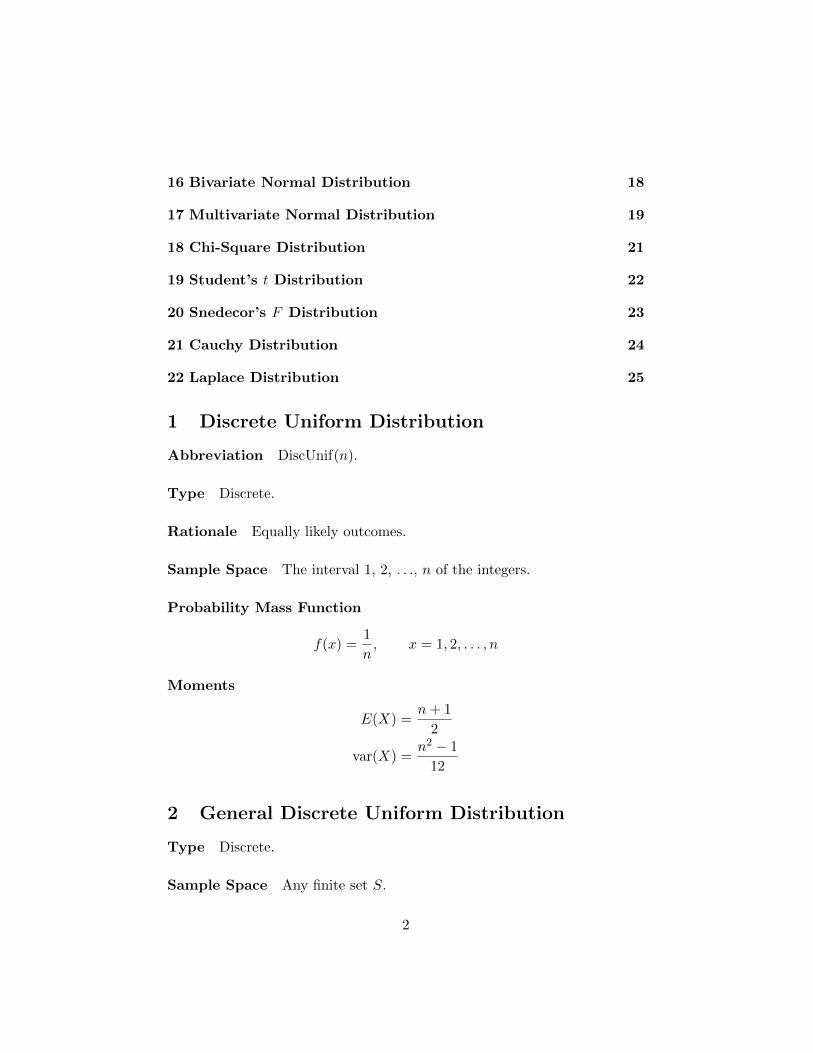
16 Bivariate Normal Distribution 18
17 Multivariate Normal Distribution 19
18 Chi-Square Distribution 21
19 Student’s t Distribution 22
20 Snedecor’s F Distribution 23
21 Cauchy Distribution 24
22 Laplace Distribution 25
1 Discrete Uniform Distribution
Abbreviation DiscUnif(n).
Type Discrete.
Rationale Equally likely outcomes.
Sample Space The interval 1, 2, . . ., n of the integers.
Probability Mass Function
f(x) =1
n, x = 1, 2, . . . , n
Moments
E(X) =n+ 1
2
var(X) =n2 − 1
12
2 General Discrete Uniform Distribution
Type Discrete.
Sample Space Any finite set S.
2

Probability Mass Function
f(x) =1
n, x ∈ S,
where n is the number of elements of S.
3 Uniform Distribution
Abbreviation Unif(a, b).
Type Continuous.
Rationale Continuous analog of the discrete uniform distribution.
Parameters Real numbers a and b with a < b.
Sample Space The interval (a, b) of the real numbers.
Probability Density Function
f(x) =1
b− a, a < x < b
Moments
E(X) =a+ b
2
var(X) =(b− a)2
12
Relation to Other Distributions Beta(1, 1) = Unif(0, 1).
4 General Uniform Distribution
Type Continuous.
Sample Space Any open set S in Rn.
3

Probability Density Function
f(x) =1
c, x ∈ S
where c is the measure (length in one dimension, area in two, volume inthree, etc.) of the set S.
5 Bernoulli Distribution
Abbreviation Ber(p).
Type Discrete.
Rationale Any zero-or-one-valued random variable.
Parameter Real number 0 ≤ p ≤ 1.
Sample Space The two-element set {0, 1}.
Probability Mass Function
f(x) =
{p, x = 1
1− p, x = 0
Moments
E(X) = p
var(X) = p(1− p)
Addition Rule If X1, . . ., Xk are IID Ber(p) random variables, thenX1 + · · ·+Xk is a Bin(k, p) random variable.
Degeneracy If p = 0 the distribution is concentrated at 0. If p = 1 thedistribution is concentrated at 1.
Relation to Other Distributions Ber(p) = Bin(1, p).
4
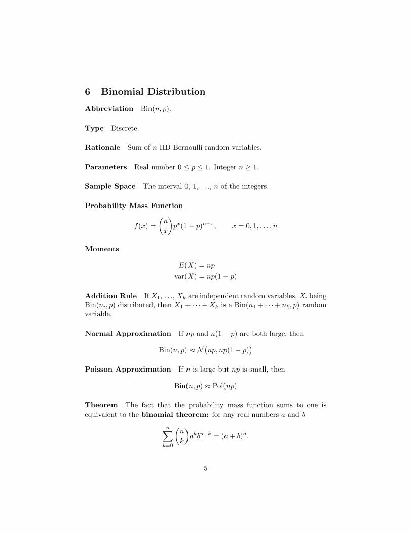
6 Binomial Distribution
Abbreviation Bin(n, p).
Type Discrete.
Rationale Sum of n IID Bernoulli random variables.
Parameters Real number 0 ≤ p ≤ 1. Integer n ≥ 1.
Sample Space The interval 0, 1, . . ., n of the integers.
Probability Mass Function
f(x) =
(n
x
)px(1− p)n−x, x = 0, 1, . . . , n
Moments
E(X) = np
var(X) = np(1− p)
Addition Rule If X1, . . ., Xk are independent random variables, Xi beingBin(ni, p) distributed, then X1 + · · ·+Xk is a Bin(n1 + · · ·+ nk, p) randomvariable.
Normal Approximation If np and n(1− p) are both large, then
Bin(n, p) ≈ N(np, np(1− p)
)Poisson Approximation If n is large but np is small, then
Bin(n, p) ≈ Poi(np)
Theorem The fact that the probability mass function sums to one isequivalent to the binomial theorem: for any real numbers a and b
n∑k=0
(n
k
)akbn−k = (a+ b)n.
5

Degeneracy If p = 0 the distribution is concentrated at 0. If p = 1 thedistribution is concentrated at n.
Relation to Other Distributions Ber(p) = Bin(1, p).
7 Hypergeometric Distribution
Abbreviation Hypergeometric(A,B, n).
Type Discrete.
Rationale Sample of size n without replacement from finite population ofB zeros and A ones.
Sample Space The interval max(0, n−B), . . ., min(n,A) of the integers.
Probability Mass Function
f(x) =
(Ax
)(Bn−x)(
A+Bn
) , x = max(0, n−B), . . . ,min(n,A)
Moments
E(X) = np
var(X) = np(1− p) · N − nN − 1
where
p =A
A+B(7.1)
N = A+B
Binomial Approximation If n is small compared to either A or B, then
Hypergeometric(n,A,B) ≈ Bin(n, p)
where p is given by (7.1).
6

Normal Approximation If n is large, but small compared to either Aor B, then
Hypergeometric(n,A,B) ≈ N(np, np(1− p)
)where p is given by (7.1).
Theorem The fact that the probability mass function sums to one isequivalent to
min(A,n)∑x=max(0,n−B)
(A
x
)(B
n− x
)=
(A+B
n
)
8 Poisson Distribution
Abbreviation Poi(µ)
Type Discrete.
Rationale Counts in a Poisson process.
Parameter Real number µ > 0.
Sample Space The non-negative integers 0, 1, . . . .
Probability Mass Function
f(x) =µx
x!e−µ, x = 0, 1, . . .
Moments
E(X) = µ
var(X) = µ
Addition Rule If X1, . . ., Xk are independent random variables, Xi beingPoi(µi) distributed, then X1+· · ·+Xk is a Poi(µ1+· · ·+µk) random variable.
Normal Approximation If µ is large, then
Poi(µ) ≈ N (µ, µ)
7
Theorem The fact that the probability mass function sums to one isequivalent to the Maclaurin series for the exponential function: for anyreal number x
∞∑k=0
xk
k!= ex.
9 Geometric Distribution
Abbreviation Geo(p).
Type Discrete.
Rationales
• Discrete lifetime of object that does not age.
• Waiting time or interarrival time in sequence of IID Bernoulli trials.
• Inverse sampling.
• Discrete analog of the exponential distribution.
Parameter Real number 0 < p ≤ 1.
Sample Space The non-negative integers 0, 1, . . . .
Probability Mass Function
f(x) = p(1− p)x x = 0, 1, . . .
Moments
E(X) =1− pp
var(X) =1− pp2
Addition Rule If X1, . . ., Xk are IID Geo(p) random variables, thenX1 + · · ·+Xk is a NegBin(k, p) random variable.
8

Theorem The fact that the probability mass function sums to one isequivalent to the geometric series: for any real number s such that |s| < 1
∞∑k=0
sk =1
1− s.
Degeneracy If p = 1 the distribution is concentrated at 0.
10 Negative Binomial Distribution
Abbreviation NegBin(r, p).
Type Discrete.
Rationale
• Sum of IID geometric random variables.
• Inverse sampling.
• Gamma mixture of Poisson distributions.
Parameters Real number 0 < p ≤ 1. Integer r ≥ 1.
Sample Space The non-negative integers 0, 1, . . . .
Probability Mass Function
f(x) =
(r + x− 1
x
)pr(1− p)x, x = 0, 1, . . .
Moments
E(X) =r(1− p)
p
var(X) =r(1− p)p2
Addition Rule If X1, . . ., Xk are independent random variables, Xi beingNegBin(ri, p) distributed, then X1 + · · · + Xk is a NegBin(r1 + · · · + rk, p)random variable.
9
Normal Approximation If r(1− p) is large, then
NegBin(r, p) ≈ N(r(1− p)
p,r(1− p)p2
)Degeneracy If p = 1 the distribution is concentrated at 0.
Extended Definition The definition makes sense for noninteger r if bi-nomial coefficients are defined by(
r
k
)=r · (r − 1) · · · (r − k + 1)
k!
which for integer r agrees with the standard definition.Also (
r + x− 1
x
)= (−1)x
(−rx
)(10.1)
which explains the name “negative binomial.”
Theorem The fact that the probability mass function sums to one isequivalent to the generalized binomial theorem: for any real numbers such that −1 < s < 1 and any real number m
∞∑k=0
(m
k
)sk = (1 + s)m. (10.2)
If m is a nonnegative integer, then(mk
)is zero for k > m, and we get the
ordinary binomial theorem.Changing variables from m to −m and from s to −s and using (10.1)
turns (10.2) into
∞∑k=0
(m+ k − 1
k
)sk =
∞∑k=0
(−mk
)(−s)k = (1− s)−m
which has a more obvious relationship to the negative binomial density sum-ming to one.
11 Normal Distribution
Abbreviation N (µ, σ2).
10
Type Continuous.
Rationale
• Limiting distribution in the central limit theorem.
• Error distribution that turns the method of least squares into maxi-mum likelihood estimation.
Parameters Real numbers µ and σ2 > 0.
Sample Space The real numbers.
Probability Density Function
f(x) =1√2πσ
e−(x−µ)2/2σ2
, −∞ < x <∞
Moments
E(X) = µ
var(X) = σ2
E{(X − µ)3} = 0
E{(X − µ)4} = 3σ4
Linear Transformations If X is N (µ, σ2) distributed, then aX + b isN (aµ+ b, a2σ2) distributed.
Addition Rule If X1, . . ., Xk are independent random variables, Xi beingN (µi, σ
2i ) distributed, then X1 + · · ·+Xk is a N (µ1 + · · ·+µk, σ
21 + · · ·+σ2k)
random variable.
Theorem The fact that the probability density function integrates to oneis equivalent to the integral∫ ∞
−∞e−z
2/2 dz =√
2π
Relation to Other Distributions If Z is N (0, 1) distributed, then Z2
is Gam(12 ,12) = chi2(1) distributed. Also related to Student t, Snedecor F ,
and Cauchy distributions (for which see).
11
12 Exponential Distribution
Abbreviation Exp(λ).
Type Continuous.
Rationales
• Lifetime of object that does not age.
• Waiting time or interarrival time in Poisson process.
• Continuous analog of the geometric distribution.
Parameter Real number λ > 0.
Sample Space The interval (0,∞) of the real numbers.
Probability Density Function
f(x) = λe−λx, 0 < x <∞
Cumulative Distribution Function
F (x) = 1− e−λx, 0 < x <∞
Moments
E(X) =1
λ
var(X) =1
λ2
Addition Rule If X1, . . ., Xk are IID Exp(λ) random variables, thenX1 + · · ·+Xk is a Gam(k, λ) random variable.
Relation to Other Distributions Exp(λ) = Gam(1, λ).
13 Gamma Distribution
Abbreviation Gam(α, λ).
12
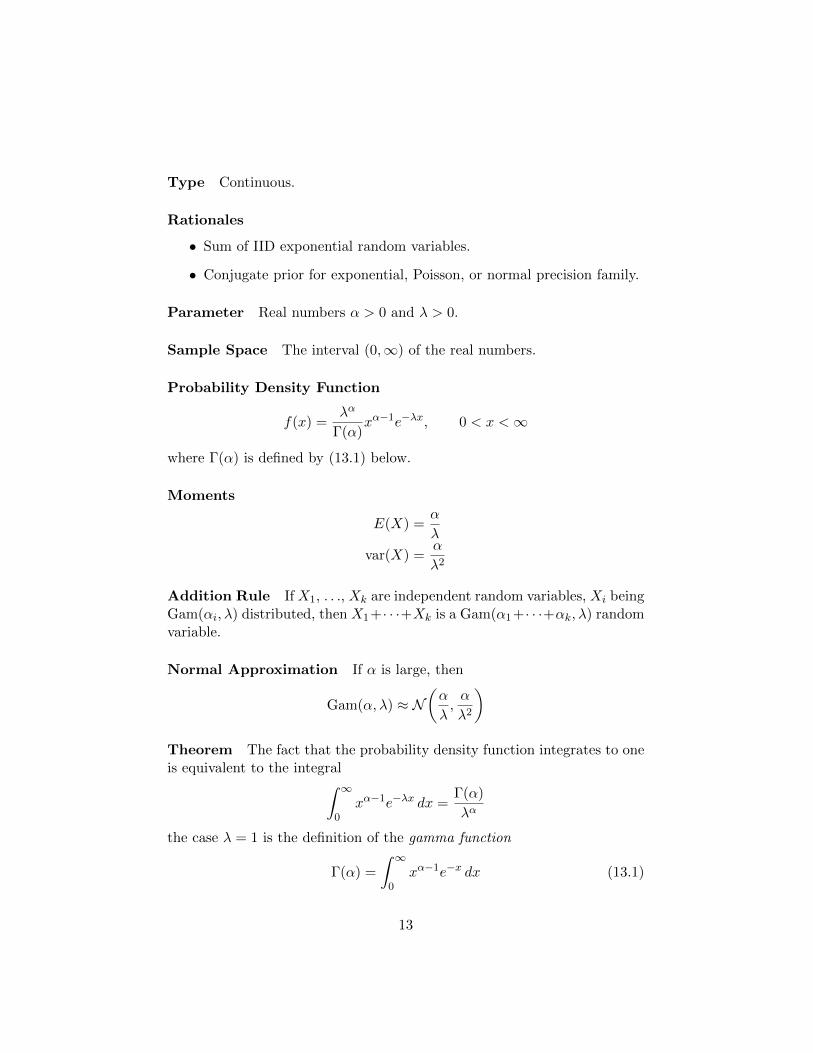
Type Continuous.
Rationales
• Sum of IID exponential random variables.
• Conjugate prior for exponential, Poisson, or normal precision family.
Parameter Real numbers α > 0 and λ > 0.
Sample Space The interval (0,∞) of the real numbers.
Probability Density Function
f(x) =λα
Γ(α)xα−1e−λx, 0 < x <∞
where Γ(α) is defined by (13.1) below.
Moments
E(X) =α
λ
var(X) =α
λ2
Addition Rule If X1, . . ., Xk are independent random variables, Xi beingGam(αi, λ) distributed, then X1+· · ·+Xk is a Gam(α1+· · ·+αk, λ) randomvariable.
Normal Approximation If α is large, then
Gam(α, λ) ≈ N(α
λ,α
λ2
)Theorem The fact that the probability density function integrates to oneis equivalent to the integral∫ ∞
0xα−1e−λx dx =
Γ(α)
λα
the case λ = 1 is the definition of the gamma function
Γ(α) =
∫ ∞0
xα−1e−x dx (13.1)
13

Relation to Other Distributions
• Exp(λ) = Gam(1, λ).
• chi2(ν) = Gam(ν2 ,12).
• IfX and Y are independent, X is Γ(α1, λ) distributed and Y is Γ(α2, λ)distributed, then X/(X + Y ) is Beta(α1, α2) distributed.
• If Z is N (0, 1) distributed, then Z2 is Gam(12 ,12) distributed.
Facts About Gamma Functions Integration by parts in (13.1) estab-lishes the gamma function recursion formula
Γ(α+ 1) = αΓ(α), α > 0 (13.2)
The relationship between the Exp(λ) and Gam(1, λ) distributions gives
Γ(1) = 1
and the relationship between the N (0, 1) and Gam(12 ,12) distributions gives
Γ(12) =√π
Together with the recursion (13.2) these give for any positive integer n
Γ(n+ 1) = n!
andΓ(n+ 1
2) =(n− 1
2
) (n− 3
2
)· · · 32 ·
12
√π
14 Beta Distribution
Abbreviation Beta(α1, α2).
Type Continuous.
Rationales
• Ratio of gamma random variables.
• Conjugate prior for binomial or negative binomial family.
14

Parameter Real numbers α1 > 0 and α2 > 0.
Sample Space The interval (0, 1) of the real numbers.
Probability Density Function
f(x) =Γ(α1 + α2)
Γ(α1)Γ(α2)xα1−1(1− x)α2−1 0 < x < 1
where Γ(α) is defined by (13.1) above.
Moments
E(X) =α1
α1 + α2
var(X) =α1α2
(α1 + α2)2(α1 + α2 + 1)
Theorem The fact that the probability density function integrates to oneis equivalent to the integral∫ 1
0xα1−1(1− x)α2−1 dx =
Γ(α1)Γ(α2)
Γ(α1 + α2)
Relation to Other Distributions
• IfX and Y are independent, X is Γ(α1, λ) distributed and Y is Γ(α2, λ)distributed, then X/(X + Y ) is Beta(α1, α2) distributed.
• Beta(1, 1) = Unif(0, 1).
15 Multinomial Distribution
Abbreviation Multi(n,p).
Type Discrete.
Rationale Multivariate analog of the binomial distribution.
15
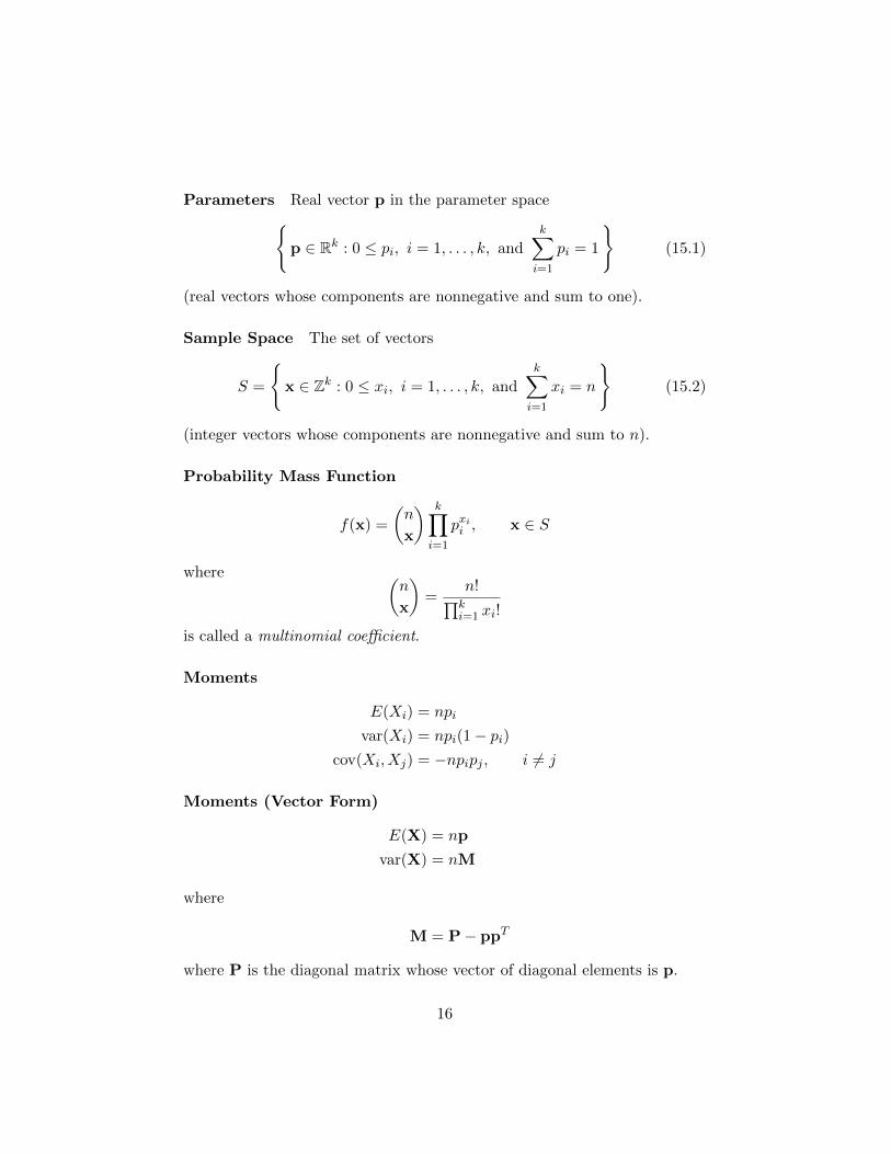
Parameters Real vector p in the parameter space{p ∈ Rk : 0 ≤ pi, i = 1, . . . , k, and
k∑i=1
pi = 1
}(15.1)
(real vectors whose components are nonnegative and sum to one).
Sample Space The set of vectors
S =
{x ∈ Zk : 0 ≤ xi, i = 1, . . . , k, and
k∑i=1
xi = n
}(15.2)
(integer vectors whose components are nonnegative and sum to n).
Probability Mass Function
f(x) =
(n
x
) k∏i=1
pxii , x ∈ S
where (n
x
)=
n!∏ki=1 xi!
is called a multinomial coefficient.
Moments
E(Xi) = npi
var(Xi) = npi(1− pi)cov(Xi, Xj) = −npipj , i 6= j
Moments (Vector Form)
E(X) = np
var(X) = nM
where
M = P− ppT
where P is the diagonal matrix whose vector of diagonal elements is p.
16
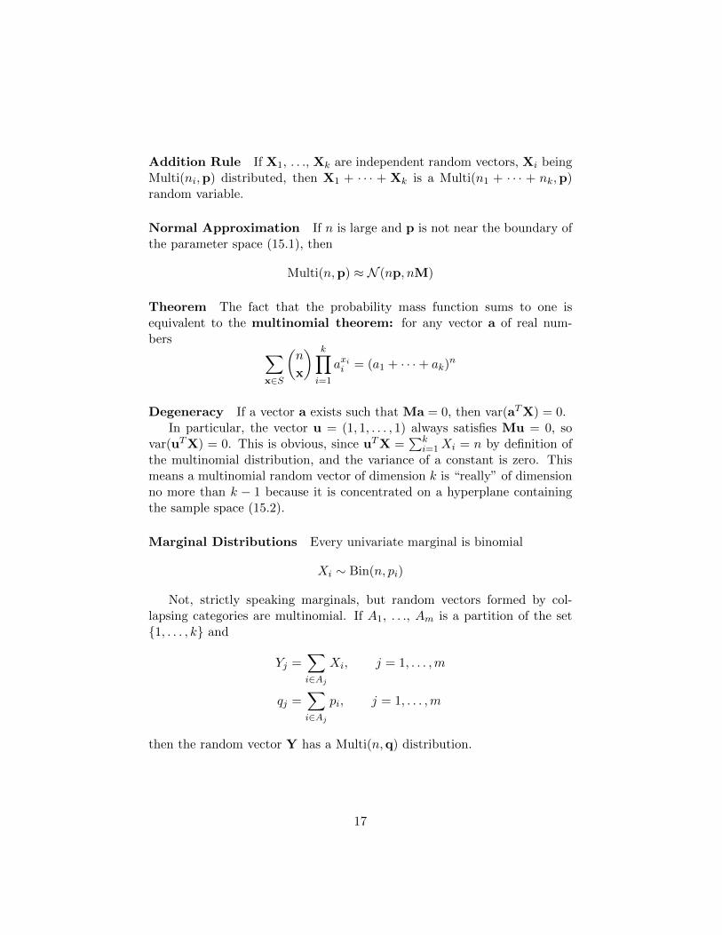
Addition Rule If X1, . . ., Xk are independent random vectors, Xi beingMulti(ni,p) distributed, then X1 + · · · + Xk is a Multi(n1 + · · · + nk,p)random variable.
Normal Approximation If n is large and p is not near the boundary ofthe parameter space (15.1), then
Multi(n,p) ≈ N (np, nM)
Theorem The fact that the probability mass function sums to one isequivalent to the multinomial theorem: for any vector a of real num-bers ∑
x∈S
(n
x
) k∏i=1
axii = (a1 + · · ·+ ak)n
Degeneracy If a vector a exists such that Ma = 0, then var(aTX) = 0.In particular, the vector u = (1, 1, . . . , 1) always satisfies Mu = 0, so
var(uTX) = 0. This is obvious, since uTX =∑k
i=1Xi = n by definition ofthe multinomial distribution, and the variance of a constant is zero. Thismeans a multinomial random vector of dimension k is “really” of dimensionno more than k − 1 because it is concentrated on a hyperplane containingthe sample space (15.2).
Marginal Distributions Every univariate marginal is binomial
Xi ∼ Bin(n, pi)
Not, strictly speaking marginals, but random vectors formed by col-lapsing categories are multinomial. If A1, . . ., Am is a partition of the set{1, . . . , k} and
Yj =∑i∈Aj
Xi, j = 1, . . . ,m
qj =∑i∈Aj
pi, j = 1, . . . ,m
then the random vector Y has a Multi(n,q) distribution.
17

Conditional Distributions If {i1, . . . , im} and {im+1, . . . , ik} partitionthe set {1, . . . , k}, then the conditional distribution of Xi1 , . . ., Xim givenXim+1 , . . ., Xik is Multi(n − Xim+1 − · · · − Xik ,q), where the parametervector q has components
qj =pij
pi1 + · · ·+ pim, j = 1, . . . ,m
Relation to Other Distributions
• Each marginal of a multinomial is binomial.
• If X is Bin(n, p), then the vector (X,n−X) is Multi(n, (p, 1− p)
).
16 Bivariate Normal Distribution
Abbreviation See multivariate normal below.
Type Continuous.
Rationales See multivariate normal below.
Parameters Real vector µ of dimension 2, real symmetric positive semi-definite matrix M of dimension 2× 2 having the form
M =
(σ21 ρσ1σ2
ρσ1σ2 σ22
)where σ1 > 0, σ2 > 0 and −1 < ρ < +1.
Sample Space The Euclidean space R2.
Probability Density Function
f(x) =1
2πdet(M)−1/2 exp
(−1
2(x− µ)TM−1(x− µ))
=1
2π√
1− ρ2σ1σ2exp
(− 1
2(1− ρ2)
[(x1 − µ1σ1
)2
−2ρ
(x1 − µ1σ1
)(x2 − µ2σ2
)+
(x2 − µ2σ2
)2])
, x ∈ R2
18

Moments
E(Xi) = µi, i = 1, 2
var(Xi) = σ2i , i = 1, 2
cov(X1, X2) = ρσ1σ2
cor(X1, X2) = ρ
Moments (Vector Form)
E(X) = µ
var(X) = M
Linear Transformations See multivariate normal below.
Addition Rule See multivariate normal below.
Marginal Distributions Xi is N (µi, σ2i ) distributed, i = 1, 2.
Conditional Distributions The conditional distribution of X2 given X1
isN(µ2 + ρ
σ2σ1
(x1 − µ1), (1− ρ2)σ22)
17 Multivariate Normal Distribution
Abbreviation N (µ,M)
Type Continuous.
Rationales
• Multivariate analog of the univariate normal distribution.
• Limiting distribution in the multivariate central limit theorem.
Parameters Real vector µ of dimension k, real symmetric positive semi-definite matrix M of dimension k × k.
Sample Space The Euclidean space Rk.
19
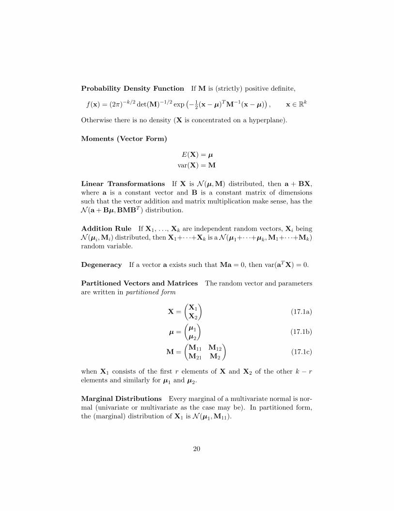
Probability Density Function If M is (strictly) positive definite,
f(x) = (2π)−k/2 det(M)−1/2 exp(−1
2(x− µ)TM−1(x− µ)), x ∈ Rk
Otherwise there is no density (X is concentrated on a hyperplane).
Moments (Vector Form)
E(X) = µ
var(X) = M
Linear Transformations If X is N (µ,M) distributed, then a + BX,where a is a constant vector and B is a constant matrix of dimensionssuch that the vector addition and matrix multiplication make sense, has theN (a + Bµ,BMBT ) distribution.
Addition Rule If X1, . . ., Xk are independent random vectors, Xi beingN (µi,Mi) distributed, then X1+· · ·+Xk is aN (µ1+· · ·+µk,M1+· · ·+Mk)random variable.
Degeneracy If a vector a exists such that Ma = 0, then var(aTX) = 0.
Partitioned Vectors and Matrices The random vector and parametersare written in partitioned form
X =
(X1
X2
)(17.1a)
µ =
(µ1
µ2
)(17.1b)
M =
(M11 M12
M21 M2
)(17.1c)
when X1 consists of the first r elements of X and X2 of the other k − relements and similarly for µ1 and µ2.
Marginal Distributions Every marginal of a multivariate normal is nor-mal (univariate or multivariate as the case may be). In partitioned form,the (marginal) distribution of X1 is N (µ1,M11).
20

Conditional Distributions Every conditional of a multivariate normalis normal (univariate or multivariate as the case may be). In partitionedform, the conditional distribution of X1 given X2 is
N (µ1 + M12M−22[X2 − µ2],M11 −M12M
−22M21)
where the notation M−22 denotes the inverse of the matrix M−
22 if the matrixis invertible and otherwise any generalized inverse.
18 Chi-Square Distribution
Abbreviation chi2(ν) or χ2(ν).
Type Continuous.
Rationales
• Sum of squares of IID standard normal random variables.
• Sampling distribution of sample variance when data are IID normal.
• Asymptotic distribution in Pearson chi-square test.
• Asymptotic distribution of log likelihood ratio.
Parameter Real number ν > 0 called “degrees of freedom.”
Sample Space The interval (0,∞) of the real numbers.
Probability Density Function
f(x) =(12)ν/2
Γ(ν2 )xν/2−1e−x/2, 0 < x <∞.
Moments
E(X) = ν
var(X) = 2ν
Addition Rule If X1, . . ., Xk are independent random variables, Xi beingchi2(νi) distributed, thenX1+· · ·+Xk is a chi2(ν1+· · ·+νk) random variable.
21

Normal Approximation If ν is large, then
chi2(ν) ≈ N (ν, 2ν)
Relation to Other Distributions
• chi2(ν) = Gam(ν2 ,12).
• If X is N (0, 1) distributed, then X2 is chi2(1) distributed.
• If Z and Y are independent, X is N (0, 1) distributed and Y is chi2(ν)distributed, then X/
√Y/ν is t(ν) distributed.
• If X and Y are independent and are chi2(µ) and chi2(ν) distributed,respectively, then (X/µ)/(Y/ν) is F (µ, ν) distributed.
19 Student’s t Distribution
Abbreviation t(ν).
Type Continuous.
Rationales
• Sampling distribution of pivotal quantity√n(Xn − µ)/Sn when data
are IID normal.
• Marginal for µ in conjugate prior family for two-parameter normaldata.
Parameter Real number ν > 0 called “degrees of freedom.”
Sample Space The real numbers.
Probability Density Function
f(x) =1√νπ·
Γ(ν+12 )
Γ(ν2 )· 1(
1 + x2
ν
)(ν+1)/2, −∞ < x < +∞
22

Moments If ν > 1, thenE(X) = 0.
Otherwise the mean does not exist. If ν > 2, then
var(X) =ν
ν − 2.
Otherwise the variance does not exist.
Normal Approximation If ν is large, then
t(ν) ≈ N (0, 1)
Relation to Other Distributions
• If X and Y are independent, X is N (0, 1) distributed and Y is chi2(ν)distributed, then X/
√Y/ν is t(ν) distributed.
• If X is t(ν) distributed, then X2 is F (1, ν) distributed.
• t(1) = Cauchy(0, 1).
20 Snedecor’s F Distribution
Abbreviation F (µ, ν).
Type Continuous.
Rationale
• Ratio of sums of squares for normal data (test statistics in regressionand analysis of variance).
Parameters Real numbers µ > 0 and ν > 0 called “numerator degrees offreedom” and “denominator degrees of freedom,” respectively.
Sample Space The interval (0,∞) of the real numbers.
Probability Density Function
f(x) =Γ(µ+ν2 )µµ/2νν/2
Γ(µ2 )Γ(ν2 )· xµ/2−1
(µx+ ν)(µ+ν)/2, 0 < x < +∞
23

Moments If ν > 2, then
E(X) =ν
ν − 2.
Otherwise the mean does not exist.
Relation to Other Distributions
• If X and Y are independent and are chi2(µ) and chi2(ν) distributed,respectively, then (X/µ)/(Y/ν) is F (µ, ν) distributed.
• If X is t(ν) distributed, then X2 is F (1, ν) distributed.
21 Cauchy Distribution
Abbreviation Cauchy(µ, σ).
Type Continuous.
Rationales
• Very heavy tailed distribution.
• Counterexample to law of large numbers.
Parameters Real numbers µ and σ > 0.
Sample Space The real numbers.
Probability Density Function
f(x) =1
πσ· 1
1 +(x−µ
σ
)2 , −∞ < x < +∞
Moments No moments exist.
Addition Rule If X1, . . ., Xk are IID Cauchy(µ, σ) random variables,then Xn = (X1 + · · ·+Xk)/n is also Cauchy(µ, σ).
24
Relation to Other Distributions
• t(1) = Cauchy(0, 1).
22 Laplace Distribution
Abbreviation Laplace(µ, σ).
Type Continuous.
Rationales The sample median is the maximum likelihood estimate ofthe location parameter.
Parameters Real numbers µ and σ > 0, called the mean and standarddeviation, respectively.
Sample Space The real numbers.
Probability Density Function
f(x) =
√2
2σexp
(−√
2
∣∣∣∣x− µσ∣∣∣∣) , −∞ < x <∞
Moments
E(X) = µ
var(X) = σ2
25