Stat 3701 Lecture Notes: DataCharles J. Geyer

April 11, 2017

The combination of some data and an aching desire for an answer does not ensure that a reasonableanswer can be extracted from a given body of data.— John W. Tukey (the first of six “basics” against statistician’s hubrises) in “Sunset Salvo”,American Statistician, 40, 72–76 (1986).quoted by the fortunes package

Figure 1: xkcd:1781 Artifacts

1 License

This work is licensed under a Creative Commons Attribution-ShareAlike 4.0 International License (http://creativecommons.org/licenses/by-sa/4.0/).

1

2 R

• The version of R used to make this document is 3.3.3.

• The version of the rmarkdown package used to make this document is 1.4.

• The version of the MASS package used to make this document is 7.3.45.

• The version of the quantreg package used to make this document is 5.29.

• The version of the XML package used to make this document is 3.98.1.5.

• The version of the jsonlite package used to make this document is 1.3.

• The version of the RSQLite package used to make this document is 1.1.2.

• The version of the DBI package used to make this document is 0.6.

3 Data

3.1 Data Frames

Statistics or “data science” starts with data. Data can come in many forms but it often comes in a dataframe — or at least something R can turn into a data frame. As we saw at the end of the handout aboutmatrices, arrays, and data frames, the two R functions most commonly used to input data into data framesare read.table and read.csv. We will see some more later.

3.2 Data Artifacts, Errors, Problems

3.2.1 Introduction

Anything which uses science as part of its name isn’t: political science, creation science, computerscience.— Hal Abelson

Presumably he would have added “data science” if the term had existed when he said that. Statistics doesn’tget off lightly either because of the journal Statistical Science.

It is the dirty little secret of science, business, statistics, and “data science” is that there are a lot of errors inalmost all data when they get to a data analyst, whatever his or her job title may be.

Hence, the most important skill of a data analyst (whatever his or her job title may be) is IMHO knowinghow to find errors in data. If you can’t do that, anything else you may be able to do has no point. GIGO.

But this is a secret because businesses don’t like to admit they make errors, and neither do scientists oranyone else who generates data. So the data clean up always takes place behind the scenes. Any publiclyavailable data set has already been cleaned up.

Thus we look at a made-up data set (I took an old data set, the R dataset growth in the CRAN package fdaand introduced errors of the kind I have seen in real data sets).

As we shall see. There are no R functions or packages that help with data errors. You just have to thinkhard and use logic (both logic in your thinking and R logical operators).

2

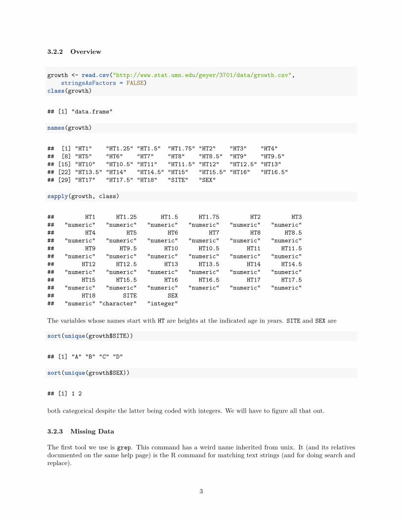
3.2.2 Overview

growth <- read.csv("http://www.stat.umn.edu/geyer/3701/data/growth.csv",stringsAsFactors = FALSE)

class(growth)

## [1] "data.frame"

names(growth)

## [1] "HT1" "HT1.25" "HT1.5" "HT1.75" "HT2" "HT3" "HT4"## [8] "HT5" "HT6" "HT7" "HT8" "HT8.5" "HT9" "HT9.5"## [15] "HT10" "HT10.5" "HT11" "HT11.5" "HT12" "HT12.5" "HT13"## [22] "HT13.5" "HT14" "HT14.5" "HT15" "HT15.5" "HT16" "HT16.5"## [29] "HT17" "HT17.5" "HT18" "SITE" "SEX"

sapply(growth, class)

## HT1 HT1.25 HT1.5 HT1.75 HT2 HT3## "numeric" "numeric" "numeric" "numeric" "numeric" "numeric"## HT4 HT5 HT6 HT7 HT8 HT8.5## "numeric" "numeric" "numeric" "numeric" "numeric" "numeric"## HT9 HT9.5 HT10 HT10.5 HT11 HT11.5## "numeric" "numeric" "numeric" "numeric" "numeric" "numeric"## HT12 HT12.5 HT13 HT13.5 HT14 HT14.5## "numeric" "numeric" "numeric" "numeric" "numeric" "numeric"## HT15 HT15.5 HT16 HT16.5 HT17 HT17.5## "numeric" "numeric" "numeric" "numeric" "numeric" "numeric"## HT18 SITE SEX## "numeric" "character" "integer"

The variables whose names start with HT are heights at the indicated age in years. SITE and SEX are

sort(unique(growth$SITE))

## [1] "A" "B" "C" "D"

sort(unique(growth$SEX))

## [1] 1 2

both categorical despite the latter being coded with integers. We will have to figure all that out.

3.2.3 Missing Data

The first tool we use is grep. This command has a weird name inherited from unix. It (and its relativesdocumented on the same help page) is the R command for matching text strings (and for doing search andreplace).

3

is.ht <- grep("HT", names(growth))foo <- growth[is.ht]foo <- as.matrix(foo)apply(foo, 2, range)

## HT1 HT1.25 HT1.5 HT1.75 HT2 HT3 HT4 HT5 HT6 HT7 HT8 HT8.5 HT9## [1,] NA NA 0.0 NA 0.0 NA NA NA NA NA 110.9 NA NA## [2,] NA NA 95.4 NA 97.3 NA NA NA NA NA 313.8 NA NA## HT9.5 HT10 HT10.5 HT11 HT11.5 HT12 HT12.5 HT13 HT13.5 HT14 HT14.5## [1,] 103.3 126.8 NA NA 0.0 NA -999.0 NA NA NA NA## [2,] 318.6 611.5 NA NA 519.7 NA 512.5 NA NA NA NA## HT15 HT15.5 HT16 HT16.5 HT17 HT17.5 HT18## [1,] NA NA NA 152.6 NA 107.0 NA## [2,] NA NA NA 255.6 NA 617.8 NA

Try again.

apply(foo, 2, range, na.rm = TRUE)

## HT1 HT1.25 HT1.5 HT1.75 HT2 HT3 HT4 HT5 HT6 HT7 HT8## [1,] -999.0 -999.0 0.0 9.4 0.0 39.6 -999.0 0 -999 -999.0 110.9## [2,] 84.1 90.4 95.4 95.0 97.3 201.3 120.6 210 134 218.8 313.8## HT8.5 HT9 HT9.5 HT10 HT10.5 HT11 HT11.5 HT12 HT12.5 HT13 HT13.5## [1,] 119.2 121.4 103.3 126.8 -999.0 -999.0 0.0 -999 -999.0 139.5 -999.0## [2,] 236.6 312.8 318.6 611.5 166.1 410.5 519.7 176 512.5 257.0 714.9## HT14 HT14.5 HT15 HT15.5 HT16 HT16.5 HT17 HT17.5 HT18## [1,] 145.0 -999.0 150.8 152.1 -999.0 152.6 0.0 107.0 0## [2,] 268.8 614.9 285.6 192.2 715.5 255.6 616.9 617.8 819

Clearly −999 and 0 are not valid heights. What’s going on?

Many statistical computing systems — I don’t want to say “languages” because many competitors to R arenot real computer languages — do not have a built-in way to handle missing data, like R’s predecessor S hashad since its beginning. So users pick an impossible value to indicate missing data. But why some NA, some−999, and some 0?

hasNA <- apply(foo, 1, anyNA)has999 <- apply(foo == (-999), 1, any)has0 <- apply(foo == 0, 1, any)sort(unique(growth$SITE[hasNA]))

## [1] "C" "D"

sort(unique(growth$SITE[has999]))

## [1] "A"

sort(unique(growth$SITE[has0]))

## [1] "B"

4

So clearly the different “sites” coded missing data differently. Now that we understand that we can

• fix the different missing data codes, and

• be on the lookout for what else the different “sites” may have done differently.

Fix.

foo[foo == -999] <- NAfoo[foo == 0] <- NAmin(foo, na.rm = TRUE)

## [1] 9.4

3.2.4 Impossible Data

3.2.4.1 Finding the Problems

Clearly, people don’t decrease in height as they age (at least when they are young). So that is another sanitycheck.

bar <- apply(foo, 1, diff)sum(bar < 0)

## [1] NA

Hmmmmm. Didn’t work because of the missing data. Try again.

bar <- apply(foo, 1, function(x) {x <- x[! is.na(x)]diff(x)

})class(bar)

## [1] "list"

according to the documentation to apply it returns a list when the function returns vectors of differentlengths for different “margins” (here rows).

any(sapply(bar, function(x) any(x < 0)))

## [1] TRUE

So we do have some impossible data. Is it just slightly impossible or very impossible?

baz <- sort(unlist(lapply(bar, function(x) x[x < 0])))length(baz)

## [1] 186

5

range(baz)

## [1] -539.4 -0.1

The -0.1 may be a negligible error, but the -539.4 is highly impossible. We’ve got work to do on this issue.

3.2.4.2 Fixing the Problems

At this point anyone (even me) would be tempted to just give up using R or any other computer language towork on this issue. It is just too messy. Suck the data into a spreadsheet or other error, fix it by hand, andbe done with it.

But this is not reproducible and not scalable. There is no way anyone (even the person doing the dataediting) can reproduce exactly what they did or explain what they did. So why should we trust that? Weshouldn’t. Moreover, for “big data” it is a nonstarter. A human can fix a little bit of the data, but we needan automatic process if we are going to fix all the data. Hence we keep plugging away with R.

Any negative increment between heights may be because of either of the heights being subtracted beingwrong. And just looking at those two numbers, we cannot tell which is wrong. So let us also look at he twonumbers to either side (if there are such).

This job is so messy I think we need loops.

qux <- NULLfor (i in 1:nrow(foo))

for (j in seq(1, ncol(foo) - 1))if (foo[i, j + 1] < foo[i, j]) {

below <- if (j - 1 >= 1) foo[i, j - 1] else NAabove <- if (j + 2 <= ncol(foo)) foo[i, j + 2] else NAqux <- rbind(qux, c(below, foo[i, j], foo[i, j + 1], above))

}

## Error in if (foo[i, j + 1] < foo[i, j]) {: missing value where TRUE/FALSE needed

qux

## HT1 HT1.25 HT1.5 HT1.75## [1,] 73.8 78.7 38 85.8

That didn’t work. Forgot about the NA’s. Try again.

qux <- NULLfor (i in 1:nrow(foo)) {

x <- foo[i, ]x <- x[! is.na(x)]d <- diff(x)jj <- which(d < 0)for (j in jj) {

below <- if (j - 1 >= 1) x[j - 1] else NAabove <- if (j + 2 <= length(x)) x[j + 2] else NAqux <- rbind(qux, c(below, x[j], x[j + 1], above))

}}qux

6

## HT1 HT1.25 HT1.5 HT1.75## [1,] 73.8 78.7 38.0 85.8## [2,] 171.1 185.2 180.8 182.2## [3,] 104.1 121.5 119.0 128.0## [4,] 136.6 149.5 141.9 144.8## [5,] 152.3 156.3 116.2 165.9## [6,] 177.3 177.6 177.3 177.0## [7,] 177.6 177.3 177.0 177.0## [8,] 131.4 144.3 136.8 139.7## [9,] 154.0 518.0 162.1 166.5## [10,] 153.3 157.7 152.3 166.1## [11,] 171.1 714.9 177.9 180.1## [12,] 165.5 196.7 173.1 175.6## [13,] 179.3 189.8 180.3 180.7## [14,] 134.1 137.1 104.2 413.0## [15,] 104.2 413.0 145.7 148.5## [16,] 158.4 161.2 155.2 166.0## [17,] 119.4 221.9 124.2 126.3## [18,] 140.5 243.6 146.8 149.0## [19,] 164.2 164.6 163.9 165.0## [20,] 137.1 139.5 132.9 145.0## [21,] 161.8 262.8 163.5 164.0## [22,] 161.4 262.4 163.4 154.0## [23,] 262.4 163.4 154.0 164.3## [24,] 142.7 146.1 140.9 254.1## [25,] 140.9 254.1 158.8 160.4## [26,] 163.0 163.1 163.0 163.1## [27,] 163.7 163.8 163.7 NA## [28,] 78.3 92.4 87.2 91.4## [29,] 170.4 171.3 127.0 162.7## [30,] 129.8 312.8 125.2 137.6## [31,] 75.9 79.4 72.1 85.7## [32,] 115.3 124.0 103.6 137.6## [33,] 144.8 248.0 151.8 155.3## [34,] 175.8 176.1 176.0 NA## [35,] 143.0 164.7 150.5 153.7## [36,] 218.8 313.8 136.9 139.9## [37,] 172.2 172.3 171.2 172.5## [38,] 110.0 116.1 110.9 123.6## [39,] 150.3 161.0 151.4 151.7## [40,] 86.2 96.5 14.1 110.8## [41,] 125.2 310.9 133.4 135.9## [42,] 173.8 175.0 174.7 176.1## [43,] 176.5 616.9 177.2 177.5## [44,] 168.1 168.4 158.9 169.4## [45,] 116.2 134.0 131.1 136.8## [46,] 148.1 161.3 154.8 158.5## [47,] 158.4 171.7 164.2 165.6## [48,] 179.6 189.2 181.6 NA## [49,] 149.6 162.2 155.3 159.2## [50,] 176.1 178.3 177.9 178.2## [51,] 81.3 85.1 39.6 101.9## [52,] 130.9 143.1 137.8 139.3## [53,] 151.7 155.0 148.9 163.3

7

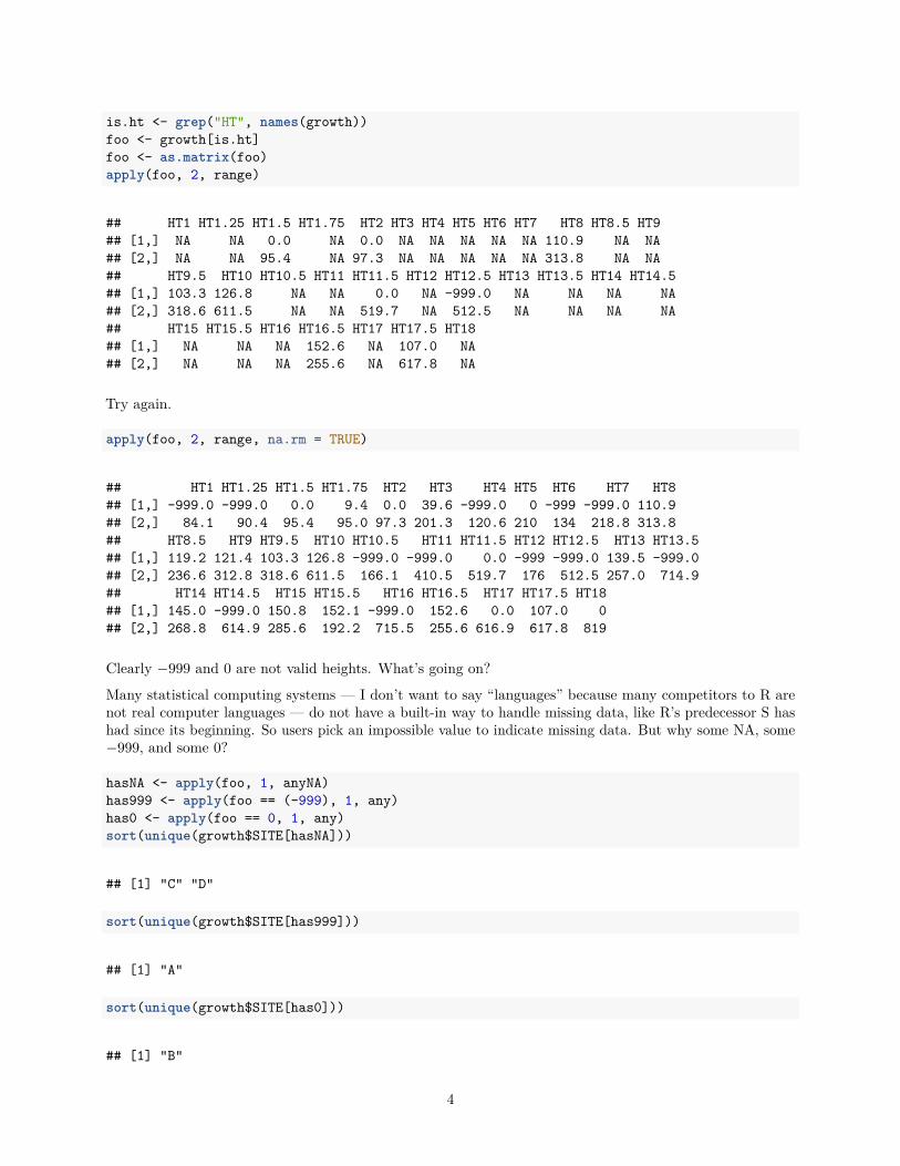
## [54,] 91.4 201.3 108.0 121.5## [55,] 163.6 166.6 160.9 175.0## [56,] 78.0 80.6 48.4 90.2## [57,] 175.5 176.0 166.4 NA## [58,] 165.9 166.1 166.0 176.0## [59,] 81.8 95.4 77.9 89.6## [60,] 161.8 161.8 161.7 161.9## [61,] 161.9 161.9 161.7 161.9## [62,] 106.7 123.3 118.4 124.2## [63,] 164.4 165.8 164.9 NA## [64,] 154.2 257.0 159.0 160.5## [65,] 163.0 163.4 163.1 163.0## [66,] 163.4 163.1 163.0 NA## [67,] 153.6 154.1 145.4 154.6## [68,] 135.8 318.6 141.4 144.2## [69,] 167.8 168.6 159.2 169.8## [70,] 169.8 169.8 107.0 170.3## [71,] 141.8 154.8 150.5 155.2## [72,] 168.6 617.8 169.2 NA## [73,] 85.1 87.5 87.3 105.7## [74,] 142.0 415.0 148.2 152.0## [75,] 167.6 268.8 169.5 169.9## [76,] 86.4 89.7 69.6 105.0## [77,] 105.0 112.3 110.6 124.7## [78,] 133.6 145.8 138.8 141.2## [79,] 167.3 167.3 167.2 NA## [80,] 137.4 410.5 134.3 145.9## [81,] 172.4 182.5 172.5 127.5## [82,] 182.5 172.5 127.5 NA## [83,] 79.1 91.1 84.4 87.4## [84,] 121.9 217.8 129.8 132.4## [85,] 172.6 273.2 173.8 NA## [86,] 76.0 79.4 28.0 84.2## [87,] 171.1 271.8 127.6 NA## [88,] 153.6 156.8 150.5 164.6## [89,] 184.2 285.6 186.6 187.1## [90,] 187.4 287.8 188.2 188.4## [91,] 83.7 86.3 79.8 92.2## [92,] 145.6 148.7 142.3 157.0## [93,] 162.0 176.4 169.9 172.1## [94,] 184.7 715.5 176.1 176.4## [95,] 122.7 129.9 123.1 136.2## [96,] 178.3 191.0 183.1 184.6## [97,] 78.3 82.3 68.0 89.1## [98,] 179.8 189.4 180.8 180.9## [99,] 180.8 180.9 180.8 181.3## [100,] 155.9 611.5 166.2 169.6## [101,] 174.2 174.2 174.1 NA## [102,] 76.2 90.4 83.3 85.7## [103,] 134.2 139.6 132.0 138.5## [104,] 132.0 138.5 131.6 144.9## [105,] 163.6 165.3 164.5 164.4## [106,] 165.3 164.5 164.4 164.3## [107,] 164.5 164.4 164.3 164.1

8

## [108,] 164.4 164.3 164.1 164.0## [109,] 164.3 164.1 164.0 163.8## [110,] 164.1 164.0 163.8 NA## [111,] 84.4 87.1 49.6 103.4## [112,] 128.1 230.4 133.2 135.8## [113,] 145.2 184.5 151.3 154.6## [114,] 81.3 95.0 87.6 94.6## [115,] 122.7 139.4 132.4 135.6## [116,] 159.4 159.7 150.9 160.2## [117,] 160.4 160.4 160.3 160.3## [118,] 77.0 87.5 19.1 94.0## [119,] 169.3 196.6 169.8 170.1## [120,] 170.3 180.5 170.6 170.8## [121,] 133.2 236.6 139.8 142.7## [122,] 171.5 171.5 171.4 171.2## [123,] 171.5 171.4 171.2 NA## [124,] NA 74.9 67.8 81.2## [125,] 163.6 163.7 153.8 NA## [126,] 132.6 236.1 139.4 142.4## [127,] 162.1 166.0 160.3 174.3## [128,] 180.4 180.4 180.2 180.5## [129,] 163.8 614.9 175.8 166.8## [130,] 614.9 175.8 166.8 168.9## [131,] 166.8 168.9 168.2 168.2## [132,] 168.2 168.2 168.1 NA## [133,] 142.4 154.0 148.1 151.8## [134,] 155.5 185.3 160.1 161.3## [135,] 162.3 173.0 163.3 163.6## [136,] 163.3 163.6 153.8 164.2## [137,] 152.9 153.2 143.6 154.1## [138,] 154.4 154.6 154.5 NA## [139,] 84.2 96.4 94.0 101.8## [140,] 121.9 126.8 119.3 121.9## [141,] 163.6 163.9 154.3 164.2## [142,] 154.3 164.2 164.0 NA## [143,] 161.0 161.5 161.0 161.8## [144,] 161.0 161.8 161.6 NA## [145,] 125.5 128.0 103.3 132.5## [146,] 142.1 244.2 146.4 148.9## [147,] 144.4 158.4 152.5 156.6## [148,] 156.6 611.5 166.1 170.2## [149,] 182.6 182.8 182.7 183.2## [150,] 172.6 172.9 137.1 173.3## [151,] 78.2 84.2 78.0 88.4## [152,] 168.7 169.1 160.5 169.9## [153,] 170.1 179.3 170.3 170.6## [154,] 100.2 180.0 114.9 121.2## [155,] 131.3 143.9 136.7 140.1## [156,] 156.9 157.0 156.9 NA## [157,] 152.2 163.6 154.9 155.9## [158,] 157.5 175.7 158.0 518.4## [159,] 155.1 255.6 156.0 157.1## [160,] 156.0 157.1 156.5 NA## [161,] 133.1 136.0 128.8 142.9

9

## [162,] 156.2 519.7 163.8 168.8## [163,] 162.3 177.7 171.5 174.3## [164,] 174.3 176.1 167.4 NA## [165,] NA 84.1 78.4 82.6## [166,] 123.2 129.9 123.0 136.0## [167,] 154.5 157.7 152.2 167.4## [168,] 85.0 86.4 77.1 96.2## [169,] 117.3 214.1 130.0 133.6## [170,] 148.7 252.3 154.3 158.1## [171,] 167.5 181.5 175.1 178.0## [172,] 95.6 120.1 109.2 117.5## [173,] 173.0 276.3 178.5 180.0## [174,] 180.0 181.0 171.8 182.2## [175,] 95.6 120.6 109.7 126.8## [176,] 109.7 126.8 121.7 127.2## [177,] 178.0 179.1 108.2 181.0## [178,] 118.6 133.7 126.4 129.1## [179,] 102.0 207.5 114.0 119.4## [180,] 131.6 143.0 136.5 138.8## [181,] 104.2 210.0 116.0 123.8## [182,] 150.1 512.5 155.1 158.4## [183,] 83.3 87.0 9.4 93.1## [184,] 153.4 156.1 149.3 163.7## [185,] 189.6 199.7 191.3 191.7## [186,] 136.8 239.8 142.6 145.1

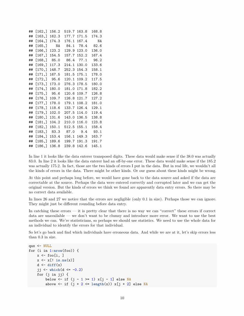
In line 1 it looks like the data enterer transposed digits. These data would make sense if the 38.0 was actually83.0. In line 2 it looks like the data enterer had an off-by-one error. These data would make sense if the 185.2was actually 175.2. In fact, those are the two kinds of errors I put in the data. But in real life, we wouldn’t allthe kinds of errors in the data. There might be other kinds. Or our guess about these kinds might be wrong.

At this point and perhaps long before, we would have gone back to the data source and asked if the data arecorrectable at the source. Perhaps the data were entered correctly and corrupted later and we can get theoriginal version. But the kinds of errors we think we found are apparently data entry errors. So there may beno correct data available.

In lines 26 and 27 we notice that the errors are negligible (only 0.1 in size). Perhaps those we can ignore.They might just be different rounding before data entry.

In catching these errors — it is pretty clear that there is no way we can “correct” these errors if correctdata are unavailable — we don’t want to be clumsy and introduce more error. We want to use the bestmethods we can. We’re statisticians, so perhaps we should use statistics. We need to use the whole data foran individual to identify the errors for that individual.

So let’s go back and find which individuals have erroneous data. And while we are at it, let’s skip errors lessthan 0.3 in size.

qux <- NULLfor (i in 1:nrow(foo)) {

x <- foo[i, ]x <- x[! is.na(x)]d <- diff(x)jj <- which(d <= -0.2)for (j in jj) {

below <- if (j - 1 >= 1) x[j - 1] else NAabove <- if (j + 2 <= length(x)) x[j + 2] else NA

10

qux <- rbind(qux, c(i, below, x[j], x[j + 1], above))}

}qux

## HT1 HT1.25 HT1.5 HT1.75## [1,] 1 73.8 78.7 38.0 85.8## [2,] 1 171.1 185.2 180.8 182.2## [3,] 2 104.1 121.5 119.0 128.0## [4,] 2 136.6 149.5 141.9 144.8## [5,] 2 152.3 156.3 116.2 165.9## [6,] 2 177.3 177.6 177.3 177.0## [7,] 2 177.6 177.3 177.0 177.0## [8,] 3 131.4 144.3 136.8 139.7## [9,] 3 154.0 518.0 162.1 166.5## [10,] 4 153.3 157.7 152.3 166.1## [11,] 6 171.1 714.9 177.9 180.1## [12,] 7 165.5 196.7 173.1 175.6## [13,] 7 179.3 189.8 180.3 180.7## [14,] 8 134.1 137.1 104.2 413.0## [15,] 8 104.2 413.0 145.7 148.5## [16,] 8 158.4 161.2 155.2 166.0## [17,] 9 119.4 221.9 124.2 126.3## [18,] 9 140.5 243.6 146.8 149.0## [19,] 10 164.2 164.6 163.9 165.0## [20,] 11 137.1 139.5 132.9 145.0## [21,] 11 161.8 262.8 163.5 164.0## [22,] 12 161.4 262.4 163.4 154.0## [23,] 12 262.4 163.4 154.0 164.3## [24,] 13 142.7 146.1 140.9 254.1## [25,] 13 140.9 254.1 158.8 160.4## [26,] 14 78.3 92.4 87.2 91.4## [27,] 14 170.4 171.3 127.0 162.7## [28,] 16 129.8 312.8 125.2 137.6## [29,] 17 75.9 79.4 72.1 85.7## [30,] 17 115.3 124.0 103.6 137.6## [31,] 17 144.8 248.0 151.8 155.3## [32,] 18 143.0 164.7 150.5 153.7## [33,] 19 218.8 313.8 136.9 139.9## [34,] 19 172.2 172.3 171.2 172.5## [35,] 20 110.0 116.1 110.9 123.6## [36,] 20 150.3 161.0 151.4 151.7## [37,] 21 86.2 96.5 14.1 110.8## [38,] 21 125.2 310.9 133.4 135.9## [39,] 21 173.8 175.0 174.7 176.1## [40,] 21 176.5 616.9 177.2 177.5## [41,] 22 168.1 168.4 158.9 169.4## [42,] 23 116.2 134.0 131.1 136.8## [43,] 23 148.1 161.3 154.8 158.5## [44,] 24 158.4 171.7 164.2 165.6## [45,] 26 179.6 189.2 181.6 NA## [46,] 27 149.6 162.2 155.3 159.2## [47,] 28 176.1 178.3 177.9 178.2

11

## [48,] 29 81.3 85.1 39.6 101.9## [49,] 29 130.9 143.1 137.8 139.3## [50,] 29 151.7 155.0 148.9 163.3## [51,] 30 91.4 201.3 108.0 121.5## [52,] 30 163.6 166.6 160.9 175.0## [53,] 31 78.0 80.6 48.4 90.2## [54,] 32 175.5 176.0 166.4 NA## [55,] 34 81.8 95.4 77.9 89.6## [56,] 34 161.9 161.9 161.7 161.9## [57,] 35 106.7 123.3 118.4 124.2## [58,] 35 164.4 165.8 164.9 NA## [59,] 36 154.2 257.0 159.0 160.5## [60,] 36 163.0 163.4 163.1 163.0## [61,] 37 153.6 154.1 145.4 154.6## [62,] 38 135.8 318.6 141.4 144.2## [63,] 38 167.8 168.6 159.2 169.8## [64,] 38 169.8 169.8 107.0 170.3## [65,] 40 141.8 154.8 150.5 155.2## [66,] 41 168.6 617.8 169.2 NA## [67,] 42 85.1 87.5 87.3 105.7## [68,] 42 142.0 415.0 148.2 152.0## [69,] 42 167.6 268.8 169.5 169.9## [70,] 43 86.4 89.7 69.6 105.0## [71,] 43 105.0 112.3 110.6 124.7## [72,] 43 133.6 145.8 138.8 141.2## [73,] 45 137.4 410.5 134.3 145.9## [74,] 45 172.4 182.5 172.5 127.5## [75,] 45 182.5 172.5 127.5 NA## [76,] 46 79.1 91.1 84.4 87.4## [77,] 46 121.9 217.8 129.8 132.4## [78,] 46 172.6 273.2 173.8 NA## [79,] 47 76.0 79.4 28.0 84.2## [80,] 47 171.1 271.8 127.6 NA## [81,] 49 153.6 156.8 150.5 164.6## [82,] 49 184.2 285.6 186.6 187.1## [83,] 49 187.4 287.8 188.2 188.4## [84,] 50 83.7 86.3 79.8 92.2## [85,] 51 145.6 148.7 142.3 157.0## [86,] 51 162.0 176.4 169.9 172.1## [87,] 51 184.7 715.5 176.1 176.4## [88,] 52 122.7 129.9 123.1 136.2## [89,] 52 178.3 191.0 183.1 184.6## [90,] 53 78.3 82.3 68.0 89.1## [91,] 53 179.8 189.4 180.8 180.9## [92,] 54 155.9 611.5 166.2 169.6## [93,] 55 76.2 90.4 83.3 85.7## [94,] 56 134.2 139.6 132.0 138.5## [95,] 56 132.0 138.5 131.6 144.9## [96,] 56 163.6 165.3 164.5 164.4## [97,] 56 164.4 164.3 164.1 164.0## [98,] 57 84.4 87.1 49.6 103.4## [99,] 57 128.1 230.4 133.2 135.8## [100,] 57 145.2 184.5 151.3 154.6## [101,] 58 81.3 95.0 87.6 94.6

12

## [102,] 58 122.7 139.4 132.4 135.6## [103,] 58 159.4 159.7 150.9 160.2## [104,] 59 77.0 87.5 19.1 94.0## [105,] 59 169.3 196.6 169.8 170.1## [106,] 59 170.3 180.5 170.6 170.8## [107,] 60 133.2 236.6 139.8 142.7## [108,] 60 171.5 171.4 171.2 NA## [109,] 61 NA 74.9 67.8 81.2## [110,] 61 163.6 163.7 153.8 NA## [111,] 62 132.6 236.1 139.4 142.4## [112,] 62 162.1 166.0 160.3 174.3## [113,] 62 180.4 180.4 180.2 180.5## [114,] 63 163.8 614.9 175.8 166.8## [115,] 63 614.9 175.8 166.8 168.9## [116,] 63 166.8 168.9 168.2 168.2## [117,] 64 142.4 154.0 148.1 151.8## [118,] 64 155.5 185.3 160.1 161.3## [119,] 64 162.3 173.0 163.3 163.6## [120,] 64 163.3 163.6 153.8 164.2## [121,] 66 152.9 153.2 143.6 154.1## [122,] 67 84.2 96.4 94.0 101.8## [123,] 67 121.9 126.8 119.3 121.9## [124,] 67 163.6 163.9 154.3 164.2## [125,] 68 161.0 161.5 161.0 161.8## [126,] 68 161.0 161.8 161.6 NA## [127,] 71 125.5 128.0 103.3 132.5## [128,] 71 142.1 244.2 146.4 148.9## [129,] 72 144.4 158.4 152.5 156.6## [130,] 72 156.6 611.5 166.1 170.2## [131,] 73 172.6 172.9 137.1 173.3## [132,] 74 78.2 84.2 78.0 88.4## [133,] 74 168.7 169.1 160.5 169.9## [134,] 74 170.1 179.3 170.3 170.6## [135,] 75 100.2 180.0 114.9 121.2## [136,] 76 131.3 143.9 136.7 140.1## [137,] 77 152.2 163.6 154.9 155.9## [138,] 77 157.5 175.7 158.0 518.4## [139,] 78 155.1 255.6 156.0 157.1## [140,] 78 156.0 157.1 156.5 NA## [141,] 79 133.1 136.0 128.8 142.9## [142,] 80 156.2 519.7 163.8 168.8## [143,] 81 162.3 177.7 171.5 174.3## [144,] 81 174.3 176.1 167.4 NA## [145,] 82 NA 84.1 78.4 82.6## [146,] 82 123.2 129.9 123.0 136.0## [147,] 82 154.5 157.7 152.2 167.4## [148,] 83 85.0 86.4 77.1 96.2## [149,] 83 117.3 214.1 130.0 133.6## [150,] 84 148.7 252.3 154.3 158.1## [151,] 84 167.5 181.5 175.1 178.0## [152,] 85 95.6 120.1 109.2 117.5## [153,] 85 173.0 276.3 178.5 180.0## [154,] 85 180.0 181.0 171.8 182.2## [155,] 86 95.6 120.6 109.7 126.8

13

## [156,] 86 109.7 126.8 121.7 127.2## [157,] 87 178.0 179.1 108.2 181.0## [158,] 88 118.6 133.7 126.4 129.1## [159,] 89 102.0 207.5 114.0 119.4## [160,] 89 131.6 143.0 136.5 138.8## [161,] 90 104.2 210.0 116.0 123.8## [162,] 90 150.1 512.5 155.1 158.4## [163,] 91 83.3 87.0 9.4 93.1## [164,] 91 153.4 156.1 149.3 163.7## [165,] 91 189.6 199.7 191.3 191.7## [166,] 93 136.8 239.8 142.6 145.1

So let’s try a bit of statistical modeling. We know there is a problem with individual 1, so lets work on himor her (we still don’t know what the codes are for SEX).

This is always a good idea. Focus on getting one thing right before moving on. I could tell many storiesabout people coming to me for help with data analysis, and the only problem they had was trying to do toomuch at once so there was no way to tell what was wrong with what they were doing. At the end, you needto have processed all of the data and done it automatically. But you don’t have to start that way.

So individual 1 data.

age <- as.numeric(sub("HT", "", colnames(foo)))age

## [1] 1.00 1.25 1.50 1.75 2.00 3.00 4.00 5.00 6.00 7.00 8.00## [12] 8.50 9.00 9.50 10.00 10.50 11.00 11.50 12.00 12.50 13.00 13.50## [23] 14.00 14.50 15.00 15.50 16.00 16.50 17.00 17.50 18.00

plot(age, foo[1, ], ylab = "height")

5 10 15

5010

015

0

age

heig

ht

14

It is pretty clear looking at the picture which points are the gross errors. But can we get statistics to tell usthat?

The one thing we know we don’t want to use is the usual sort of linear models (those fit by lm) because the“errors” are not normal. We want what is called “robust” or “resistant” regression.

The R command ??robust turns up the commands lqs and rlm in the MASS (a “recommended” package thatcomes with every R installation) package and the command line in the stats package (a core package thatcomes with every R installation). The line function is not going to be helpful because clearly the growthcurves curve. So we want to use either lqs or rlm. Both are complicated. Let us just try lqs because itcomes first in alphabetical order.

plot(age, foo[1, ], ylab = "height")library(MASS)lout <- lqs(foo[1, ] ~ poly(age, degree = 6))curve(predict(lout, newdata = data.frame(age = x)), add = TRUE)

5 10 15

5010

015

0

age

heig

ht

Humph! Doesn’t seem to fit these data well. Try rlm.

plot(age, foo[1, ], ylab = "height")rout <- rlm(foo[1, ] ~ poly(age, degree = 6))curve(predict(lout, newdata = data.frame(age = x)), add = TRUE)

15

5 10 15

5010

015

0

age

heig

ht

Neither of these work because polynomials don’t asymptote. Polynomial regression is a horrible tool forcurves that asymptote.

Some googling suggested the function smooth in the stats package. On reading the documentation for that,it is much more primitive and harder to use. But it may work, so let’s try it.

plot(age, foo[1, ], ylab = "height")y <- foo[1, ]x <- age[! is.na(y)]y <- y[! is.na(y)]sout <- smooth(y)sally <- splinefun(x, sout)curve(sally, add = TRUE)

16

5 10 15

5010

015

0

age

heig

ht

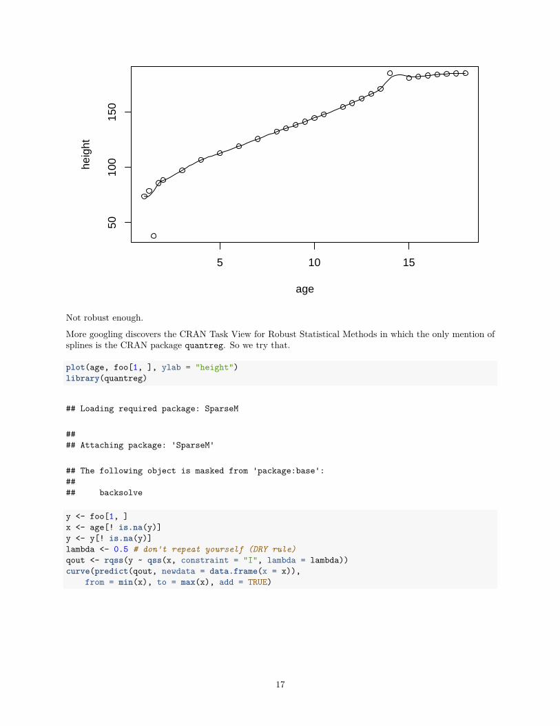
Not robust enough.

More googling discovers the CRAN Task View for Robust Statistical Methods in which the only mention ofsplines is the CRAN package quantreg. So we try that.

plot(age, foo[1, ], ylab = "height")library(quantreg)

## Loading required package: SparseM

#### Attaching package: 'SparseM'

## The following object is masked from 'package:base':#### backsolve

y <- foo[1, ]x <- age[! is.na(y)]y <- y[! is.na(y)]lambda <- 0.5 # don't repeat yourself (DRY rule)qout <- rqss(y ~ qss(x, constraint = "I", lambda = lambda))curve(predict(qout, newdata = data.frame(x = x)),

from = min(x), to = max(x), add = TRUE)

17

5 10 15

5010

015

0

age

heig

ht

The model fitting function rqss and its method for the generic function predict were a lot fussier thanthose for lqs and rlm. Like with using smooth we had to remove the NA values by hand rather than just letthe model fitting function take care of them (because rqss couldn’t take care of them and gave a completelyincomprehensible error message). And we had to add optional arguments from and to to the curve functionbecause predict.rqss refused to extrapolate beyond the range of the data (this time giving a comprehensibleerror message).

Anyway, we seem to have got what we want. Now we can compute robust residuals.

rresid <- foo[1, ] - as.numeric(predict(qout, newdata = data.frame(x = age)))rbind(height = foo[1, ], residual = rresid)

## HT1 HT1.25 HT1.5 HT1.75 HT2 HT3## height 73.80000000 78.700000 38.0000 85.8000000 8.840000e+01 97.30## residual -0.09275655 1.162221 -43.1828 0.9721773 9.355006e-11 -0.15## HT4 HT5 HT6 HT7 HT8 HT8.5## height 106.7 1.128000e+02 1.191000e+02 1.257000e+02 1.323000e+02 135.4## residual 0.2 -2.584244e-10 -2.917716e-09 3.795719e-11 3.125223e-09 0.1## HT9 HT9.5 HT10 HT10.5 HT11## height 1.383000e+02 1.413000e+02 144.7 1.479000e+02 NA## residual -2.804541e-09 -5.930048e-09 0.1 -8.265033e-11 NA## HT11.5 HT12 HT12.5 HT13## height 1.545000e+02 1.58200e+02 1.623000e+02 166.5000000## residual -1.577405e-10 -1.25624e-11 -1.904255e-12 -0.1302751## HT13.5 HT14 HT14.5 HT15 HT15.5## height 1.711000e+02 185.200000 NA 1.808000e+02 1.82200e+02## residual -2.606271e-11 9.630275 NA 4.263256e-12 -1.29603e-11## HT16 HT16.5 HT17 HT17.5## height 1.832000e+02 1.840000e+02 1.847000e+02 185.00000000## residual -3.728928e-11 -5.570655e-12 -4.279173e-10 0.01642436## HT18## height 185.20000000

18

## residual -0.03749881

The robust residuals calculated this way are all small except for the two obvious gross errors. The only onelarge in absolute value (except for the gross errors) is at the left end of the data, and this is not surprising.All smoothers have trouble at the ends where there is only data on one side to help.

In the fitting we had to choose the lambda argument to the qss function by hand (because that is whatthe help page ?qss says to do), and it did not even tell us whether large lambda means more smooth orless smooth. But with some help from what lambda does to the residuals, we got a reasonable choice (andperhaps a lot smaller would also do, but we won’t bother with more experimentation).

So let us apply this operation to all the data.

resid <- apply(foo, 1, function(y) {x <- age[! is.na(y)]y <- y[! is.na(y)]qout <- rqss(y ~ qss(x, constraint = "I", lambda = lambda))y - as.numeric(predict(qout, newdata = data.frame(x = age)))

})

## Warning in y - as.numeric(predict(qout, newdata = data.frame(x = age))):## longer object length is not a multiple of shorter object length

## Warning in y - as.numeric(predict(qout, newdata = data.frame(x = age))):## longer object length is not a multiple of shorter object length

## Warning in y - as.numeric(predict(qout, newdata = data.frame(x = age))):## longer object length is not a multiple of shorter object length

## Warning in y - as.numeric(predict(qout, newdata = data.frame(x = age))):## longer object length is not a multiple of shorter object length

## Warning in rq.fit.sfnc(x, y, tau = tau, rhs = rhs, control = control, ...):

## Warning in y - as.numeric(predict(qout, newdata = data.frame(x = age))):## longer object length is not a multiple of shorter object length

## Warning in y - as.numeric(predict(qout, newdata = data.frame(x = age))):## longer object length is not a multiple of shorter object length

## Warning in y - as.numeric(predict(qout, newdata = data.frame(x = age))):## longer object length is not a multiple of shorter object length

## Warning in y - as.numeric(predict(qout, newdata = data.frame(x = age))):## longer object length is not a multiple of shorter object length

## Warning in y - as.numeric(predict(qout, newdata = data.frame(x = age))):## longer object length is not a multiple of shorter object length

## Error in predict.qss1(qss, newdata = newd, ...): no extrapolation allowed in predict.qss

dim(foo)

19

## [1] 93 31

dim(resid)

## NULL

Didn’t work. We forgot about predict.rqss not wanting to predict beyond the range of the data (herebeyond the range of x which is the ages for which data y are not NA). We’re going to have to be trickier.

resid <- apply(foo, 1, function(y) {x <- age[! is.na(y)]y <- y[! is.na(y)]qout <- rqss(y ~ qss(x, constraint = "I", lambda = lambda))pout <- as.numeric(predict(qout, newdata = data.frame(x = x)))rout <- rep(NA, length(age))rout[match(x, age)] <- y - poutreturn(rout)

})

## Warning in rq.fit.sfnc(x, y, tau = tau, rhs = rhs, control = control, ...):

That didn’t work either. We get a very mysterious non-warning warning. The message printed above isentirely from the R function warning. It tells us what R function (one we never heard of, although it isdocumented, that is, ?rq.fit.sfnc shows a help page), but the “message” is empty. I did a little bit ofdebugging and found that the Fortran code that is called from R to do the calculations is returning animpossible error code (−17) which does not correspond to one of the documented errors. I have reportedthis as a bug to the package maintainer, and he said that somebody else had already reported it and it hasalready been fixed in the development version of the package so will be fixed in the next release.

I seem to recall not getting this message when lambda was larger. Try that.

lambda <- 0.6resid <- apply(foo, 1, function(y) {

x <- age[! is.na(y)]y <- y[! is.na(y)]qout <- rqss(y ~ qss(x, constraint = "I", lambda = lambda))pout <- as.numeric(predict(qout, newdata = data.frame(x = x)))rout <- rep(NA, length(age))rout[match(x, age)] <- y - poutreturn(rout)

})dim(foo)

## [1] 93 31

dim(resid)

## [1] 31 93

As discussed in the section about sweep in the course notes on matrices, sometimes apply returns thetranspose of what you want.

20

resid <- t(resid)

Now we need to select a cutoff

range(resid, na.rm = TRUE)

## [1] -89.25433 624.90000

stem(resid)

#### The decimal point is 2 digit(s) to the right of the |#### -0 | 9877655555## -0 | 44444443333211111111111111111111111111111111111111111111110000000000+1280## 0 | 00000000000000000000000000000000000000000000000000000000000000000000+1328## 0 | 7999## 1 | 00000000000000000000000## 1 | 8888## 2 |## 2 | 777## 3 | 1## 3 | 666## 4 | 4## 4 | 5555## 5 | 44## 5 |## 6 | 2

That didn’t show much.

bigresid <- abs(as.vector(resid))bigresid <- bigresid[bigresid > 1]stem(log10(bigresid))

#### The decimal point is 1 digit(s) to the left of the |#### 0 | 000001112222344445556666788899901111222335555555688999## 2 | 00022233466678822335677## 4 | 01224581247## 6 | 36334## 8 | 0180222333444444455555556666666777777777778888888889999999999999999## 10 | 0000000011111111234581## 12 | 2245## 14 | 233333055567## 16 | 45556633## 18 | 055615556999## 20 | 00000000000000000000## 22 | 5666## 24 | 3339666## 26 | 4555533## 28 | 0

21

That is still confusing. I had hoped there would be an obvious separation between small OK residuals (lessthan 1, which is what we have already removed) and the big bad residuals. But it seems to be a continuum.Let us decide that all of the residuals greater than 0.8 on the log scale, which is 100.8 = 6.3095734 withoutlogs are bad.

outies <- log10(abs(resid)) > 0.8outies[is.na(outies)] <- FALSEfoo[outies] <- NA

And now we should redo our whole analysis above and see how big our problems still are.

qux <- NULLfor (i in 1:nrow(foo)) {

x <- foo[i, ]x <- x[! is.na(x)]d <- diff(x)jj <- which(d <= -0.2)for (j in jj) {

below <- if (j - 1 >= 1) x[j - 1] else NAabove <- if (j + 2 <= length(x)) x[j + 2] else NAqux <- rbind(qux, c(i, below, x[j], x[j + 1], above))

}}qux

## HT16 HT16.5 HT17 HT17.5## [1,] 2 177.3 177.6 177.3 177.0## [2,] 2 177.6 177.3 177.0 177.0## [3,] 10 164.2 164.6 163.9 165.0## [4,] 19 172.2 172.3 171.2 172.5## [5,] 21 173.8 175.0 174.7 176.1## [6,] 28 176.1 178.3 177.9 178.2## [7,] 34 161.9 161.9 161.7 161.9## [8,] 35 164.4 165.8 164.9 NA## [9,] 36 163.0 163.4 163.1 163.0## [10,] 56 163.6 165.3 164.5 164.4## [11,] 56 164.4 164.3 164.1 164.0## [12,] 60 171.5 171.4 171.2 NA## [13,] 62 180.4 180.4 180.2 180.5## [14,] 63 166.8 168.9 168.2 168.2## [15,] 68 161.0 161.5 161.0 161.8## [16,] 68 161.0 161.8 161.6 NA## [17,] 74 78.2 84.2 78.0 88.4## [18,] 78 156.0 157.1 156.5 NA

Some of these look quite confusing. It is not clear what is going on. Let’s stop here, even though we are notcompletely satisfied. This is enough time spent on this one issue on a completely made up example.

3.2.5 Codes

We still have to figure out what SEX == 1 and SEX == 2 mean. And, wary of different sites doing differentthings, let us look at this per site. There should be height differences at the largest age recorded.

22

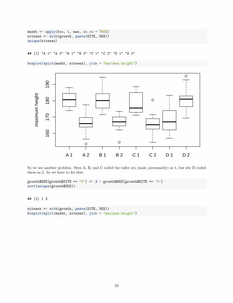
maxht <- apply(foo, 1, max, na.rm = TRUE)sitesex <- with(growth, paste(SITE, SEX))unique(sitesex)

## [1] "A 1" "A 2" "B 1" "B 2" "C 1" "C 2" "D 1" "D 2"

boxplot(split(maxht, sitesex), ylab = "maximum height")

A 1 A 2 B 1 B 2 C 1 C 2 D 1 D 2

160

170

180

190

max

imum

hei

ght

So we see another problem. Sites A, B, and C coded the taller sex (male, presumably) as 1, but site D codedthem as 2. So we have to fix that.

growth$SEX[growth$SITE == "D"] <- 3 - growth$SEX[growth$SITE == "D"]sort(unique(growth$SEX))

## [1] 1 2

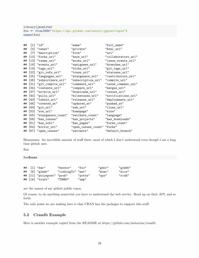
sitesex <- with(growth, paste(SITE, SEX))boxplot(split(maxht, sitesex), ylab = "maximum height")

23

A 1 A 2 B 1 B 2 C 1 C 2 D 1 D 2

160

170

180

190

max

imum

hei

ght

Looks OK now.

3.2.6 Summary

Finding errors in data is really, really hard. But it is essential.

Our example was hard, we still aren’t sure we fixed all the errors. And I cheated. I put the errors in the datain the first place, and then I went and found them (or most of them — it is just impossible to tell whethersome of the data entry errors that result in small changes are errors or not).

This example would have been much harder if I did not know what kinds of errors were in the data.

4 Data Scraping

One source of data is the World Wide Web. In general, it is very hard to read data off of web pages. Butthere is a lot to data there, so it is very useful.

The language HTML in which web pages are coded, is not that easy to parse automatically. There is a CRANpackage XML that reads and parses XML data including HTML data. But I have found it so hard to use thatI can’t actually use it (just not enough persistence, I’m sure).

Except there is one function in that package that is easy to use, so we will just illustrate that. The R functionreadHTMLTable in the R package XML finds all the HTML tables in a web page and turns each one into an Rdata frame. It returns a list, each element of which is one table in the web page.

Let’s try it. For example we will use http://www.wcha.com/women/standings.php, which is the standings forthe conference that Golden Gopher Womens’s Hockey is in.

library(XML)foo <- readHTMLTable("http://www.wcha.com/women/standings.php",

stringsAsFactors = FALSE)length(foo)

## [1] 2

24

We got two tables, and looking at the web page we see two tables, the main standings and the head-to-headtable.

foo[[1]]

## V1## 1## 2 1## 3 2## 4 3## 5 4## 6 5## 7 6## 8 7## 9 8## 10 Teams are awarded three points for each win in regulation or overtime, and one point for an overtime tie. Conference games tied after 65 minutes advance to a three-player shootout with the winning team receiving an extra point in the standings (denoted in the SW column).## V2 V3 V4 V5 V6 V7 V8 V9 V10 V11 V12 V13## 1 GP W L T SW Pts GF GA W L T## 2 Wisconsin 28 22 2 4 3 73 110 24 33 3## 3 Minnesota 28 19 4 5 3 65 88 46 26 8## 4 Minnesota Duluth 28 19 5 4 1 62 82 47 25 7## 5 North Dakota 28 11 12 5 3 41 62 57 16 16## 6 Ohio State 28 7 16 5 2 28 40 73 14 18## 7 St. Cloud State 28 7 18 3 2 26 43 82 9 23## 8 Bemidji State 28 7 18 3 1 25 49 80 12 20## 9 Minnesota State 28 4 21 3 1 16 33 98 7 26## 10 <NA> <NA> <NA> <NA> <NA> <NA> <NA> <NA> <NA> <NA> <NA> <NA>## V14 V15 V16## 1 GF GA <NA>## 2 4 157 35## 3 5 124 69## 4 5 110 62## 5 6 84 73## 6 5 69 82## 7 4 61 113## 8 3 67 90## 9 4 45 127## 10 <NA> <NA> <NA>

That didn’t work as nicely as it should have, but we did get the data. Try 2.

foo <- readHTMLTable("http://www.wcha.com/women/standings.php",stringsAsFactors = FALSE, header = TRUE)

foo[[1]]

## V1## 1## 2 1## 3 2## 4 3## 5 4## 6 5## 7 6

25

## 8 7## 9 8## 10 Teams are awarded three points for each win in regulation or overtime, and one point for an overtime tie. Conference games tied after 65 minutes advance to a three-player shootout with the winning team receiving an extra point in the standings (denoted in the SW column).## V2 V3 V4 V5 V6 V7 V8 V9 V10 V11 V12 V13## 1 GP W L T SW Pts GF GA W L T## 2 Wisconsin 28 22 2 4 3 73 110 24 33 3## 3 Minnesota 28 19 4 5 3 65 88 46 26 8## 4 Minnesota Duluth 28 19 5 4 1 62 82 47 25 7## 5 North Dakota 28 11 12 5 3 41 62 57 16 16## 6 Ohio State 28 7 16 5 2 28 40 73 14 18## 7 St. Cloud State 28 7 18 3 2 26 43 82 9 23## 8 Bemidji State 28 7 18 3 1 25 49 80 12 20## 9 Minnesota State 28 4 21 3 1 16 33 98 7 26## 10 <NA> <NA> <NA> <NA> <NA> <NA> <NA> <NA> <NA> <NA> <NA> <NA>## V14 V15 V16## 1 GF GA <NA>## 2 4 157 35## 3 5 124 69## 4 5 110 62## 5 6 84 73## 6 5 69 82## 7 4 61 113## 8 3 67 90## 9 4 45 127## 10 <NA> <NA> <NA>

That didn’t work any better. The problem is that this web site uses really crufty HTML. It doesn’t tell uswhich are the headers, the way HTML has been able to do for at least a decade. So we just have to look at itand fix it up “by hand” (in R).

foo <- foo[[1]]fooname <- foo[1, ]foobody <- foo[1 + 1:8, ]fooname

## V1 V2 V3 V4 V5 V6 V7 V8 V9 V10 V11 V12 V13 V14 V15 V16## 1 GP W L T SW Pts GF GA W L T GF GA <NA>

foobody

## V1 V2 V3 V4 V5 V6 V7 V8 V9 V10 V11 V12 V13 V14 V15 V16## 2 1 Wisconsin 28 22 2 4 3 73 110 24 33 3 4 157 35## 3 2 Minnesota 28 19 4 5 3 65 88 46 26 8 5 124 69## 4 3 Minnesota Duluth 28 19 5 4 1 62 82 47 25 7 5 110 62## 5 4 North Dakota 28 11 12 5 3 41 62 57 16 16 6 84 73## 6 5 Ohio State 28 7 16 5 2 28 40 73 14 18 5 69 82## 7 6 St. Cloud State 28 7 18 3 2 26 43 82 9 23 4 61 113## 8 7 Bemidji State 28 7 18 3 1 25 49 80 12 20 3 67 90## 9 8 Minnesota State 28 4 21 3 1 16 33 98 7 26 4 45 127

We see that web site is really crufty in its table coding. The names are off by one. And some of the namesare blank, and column 11 in the table is just empty, just there to take up space.

26

foobody <- foobody[ , -11]fooname <- fooname[-length(fooname)]fooname[1] <- "Team"fooname <- c("Place", fooname)fooname <- fooname[-11]names(foobody) <- foonamefoobody

## Place Team GP W L T SW Pts GF GA W L T GF GA## 2 1 Wisconsin 28 22 2 4 3 73 110 24 33 3 4 157 35## 3 2 Minnesota 28 19 4 5 3 65 88 46 26 8 5 124 69## 4 3 Minnesota Duluth 28 19 5 4 1 62 82 47 25 7 5 110 62## 5 4 North Dakota 28 11 12 5 3 41 62 57 16 16 6 84 73## 6 5 Ohio State 28 7 16 5 2 28 40 73 14 18 5 69 82## 7 6 St. Cloud State 28 7 18 3 2 26 43 82 9 23 4 61 113## 8 7 Bemidji State 28 7 18 3 1 25 49 80 12 20 3 67 90## 9 8 Minnesota State 28 4 21 3 1 16 33 98 7 26 4 45 127

Except that is bad because we have duplicate variable names. Looking at the table on the web, we wesee we have W, L, T, GF, GA both for play within the conference and for overall (both conference andnon-conference games). So we modify the latter.

fooname[duplicated(fooname)] <-paste(fooname[duplicated(fooname)], "O", sep = ".")

names(foobody) <- foonamefoobody

## Place Team GP W L T SW Pts GF GA W.O L.O T.O GF.O GA.O## 2 1 Wisconsin 28 22 2 4 3 73 110 24 33 3 4 157 35## 3 2 Minnesota 28 19 4 5 3 65 88 46 26 8 5 124 69## 4 3 Minnesota Duluth 28 19 5 4 1 62 82 47 25 7 5 110 62## 5 4 North Dakota 28 11 12 5 3 41 62 57 16 16 6 84 73## 6 5 Ohio State 28 7 16 5 2 28 40 73 14 18 5 69 82## 7 6 St. Cloud State 28 7 18 3 2 26 43 82 9 23 4 61 113## 8 7 Bemidji State 28 7 18 3 1 25 49 80 12 20 3 67 90## 9 8 Minnesota State 28 4 21 3 1 16 33 98 7 26 4 45 127

Better. Ugly, but usable.

5 Web Services

Some web sites have APIS that allow computers to talk to them (not just people look at them).

5.1 Github Example

Here is an example. It is copied from the vignette json-apis for the CRAN package jsonlite (for thosewho don’t know JSON is the most popular data interchange format (for computers to talk to computers)).

27

library(jsonlite)foo <- fromJSON("https://api.github.com/users/cjgeyer/repos")names(foo)

## [1] "id" "name" "full_name"## [4] "owner" "private" "html_url"## [7] "description" "fork" "url"## [10] "forks_url" "keys_url" "collaborators_url"## [13] "teams_url" "hooks_url" "issue_events_url"## [16] "events_url" "assignees_url" "branches_url"## [19] "tags_url" "blobs_url" "git_tags_url"## [22] "git_refs_url" "trees_url" "statuses_url"## [25] "languages_url" "stargazers_url" "contributors_url"## [28] "subscribers_url" "subscription_url" "commits_url"## [31] "git_commits_url" "comments_url" "issue_comment_url"## [34] "contents_url" "compare_url" "merges_url"## [37] "archive_url" "downloads_url" "issues_url"## [40] "pulls_url" "milestones_url" "notifications_url"## [43] "labels_url" "releases_url" "deployments_url"## [46] "created_at" "updated_at" "pushed_at"## [49] "git_url" "ssh_url" "clone_url"## [52] "svn_url" "homepage" "size"## [55] "stargazers_count" "watchers_count" "language"## [58] "has_issues" "has_projects" "has_downloads"## [61] "has_wiki" "has_pages" "forks_count"## [64] "mirror_url" "open_issues_count" "forks"## [67] "open_issues" "watchers" "default_branch"

Hmmmmm. An incredible amount of stuff there, most of which I don’t understand even though I am a longtime github user.

But

foo$name

## [1] "bar" "bernor" "foo" "gdor" "glmbb"## [6] "glmdr" "linkingTo" "mat" "mcmc" "nice"## [11] "polyapost" "pooh" "potts" "qux" "rcdd"## [16] "trust" "TSHRC" "ump"

are the names of my github public repos.

Of course, to do anything nontrivial you have to understand the web service. Read up on their API, and soforth.

The only point we are making here is that CRAN has the packages to support this stuff.

5.2 Crandb Example

Here is another example copied from the README at https://github.com/metacran/crandb.

28

foo <- fromJSON("http://crandb.r-pkg.org/-/latest")class(foo)

## [1] "list"

length(foo)

## [1] 10426

class(foo[[1]])

## [1] "list"

names(foo[[1]])

## [1] "Package" "Type" "Title"## [4] "Version" "Date" "Author"## [7] "Maintainer" "Description" "License"## [10] "Depends" "Suggests" "NeedsCompilation"## [13] "Packaged" "Repository" "Date/Publication"## [16] "crandb_file_date" "date" "releases"

Woof! 10426 CRAN packages as of the last time this handout was rendered.

Here’s the ones on which I am an author (I apologize for tooting my own horn).

aut <- sapply(foo, function(x) x$Author)nam <- sapply(foo, function(x) x$Package)nam[grep("Geyer", aut)]

## aster aster2 fuzzyRankTests glmbb## "aster" "aster2" "fuzzyRankTests" "glmbb"## mcmc nice polyapost pooh## "mcmc" "nice" "polyapost" "pooh"## potts rcdd trust TSHRC## "potts" "rcdd" "trust" "TSHRC"## ump## "ump"

Everything appears twice because the vectors have names and the names are the same as the values for thevector nam.

as.vector(nam[grep("Geyer", aut)])

## [1] "aster" "aster2" "fuzzyRankTests" "glmbb"## [5] "mcmc" "nice" "polyapost" "pooh"## [9] "potts" "rcdd" "trust" "TSHRC"## [13] "ump"

drops the names.

29

6 Databases

6.1 SQL Databases

A large amount of the world’s data is stored in relational database management systems (RDBMS) (Wikipediapage for that) like Oracle, MySQL, Microsoft SQL Server, PostgreSQL and IBM DB2.

The “computer language” of those thingummies is SQL (structured query language) with “computer language”in scare quotes, because it isn’t a complete computer language.

R can talk to an RDBMS via the CRAN package DBI (which we won’t illustrate).

Instead we will use the package RSQLite which talks to a very different kind of SQL database, called SQLite.

Oracle, Microsoft SQL Server, IBM DB2 are very expensive and require a lot of staff to support. The Uuses Oracle, although we say we use PeopleSoft, a company which was long ago bought by Oracle. Whenyou register for classes or get your grades. That’s PeopleSoft (Oracle). MySQL is nominally free softwarebut is owned by Oracle, and just to be safe, there are two free software clones of it (MariaDB and Percona).PostgreSQL is free software. None of these can be set up by ordinary users.

In contrast, SQLite is just a program. Any user can install it and use it. The CRAN package RSQLite hasthe SQLite RDBMS built in. So anyone can play with SQL and with R talking to RDBMS.

Once you get what you are trying to do working in RSQLite, you shouldn’t have too much trouble gettingyour R code to talk to another RDBMS via DBI except, of course, that an RDBMS like the U’s Oracledatabase won’t talk to just any program. It’s all locked up behind firewalls and other security thingummies.But assuming you do have permission to query the database using a computer, then you should be able do itusing R.

Let’s try to put our last example into an SQL database.

An SQL database has one or more tables that are more or less like data frames in R. The columns arevariables and the rows (SQL calls them tuples) are individuals (cases). Certain columns are special (primaryand secondary keys, but we won’t worry about that yet).

Since, we have to put data in tables, we have a problem. The reason fromJSON did not return a data framein the second example (Section 5.2 above) like it did in the first example (Section 5.1 above) is that the itemsin an R package description can vary.

foo.nam <- lapply(foo, names)foo.nam.union <- Reduce(union, foo.nam)foo.nam.intersection <- Reduce(intersect, foo.nam)foo.nam.union

## [1] "Package" "Type"## [3] "Title" "Version"## [5] "Date" "Author"## [7] "Maintainer" "Description"## [9] "License" "Depends"## [11] "Suggests" "NeedsCompilation"## [13] "Packaged" "Repository"## [15] "Date/Publication" "crandb_file_date"## [17] "date" "releases"## [19] "Authors@R" "URL"## [21] "BugReports" "LazyData"## [23] "VignetteBuilder" "Imports"## [25] "RoxygenNote" "Contact"## [27] "Encoding" "SystemRequirements"

30

## [29] "LazyLoad" "Lazyload"## [31] "Classification/ACM" "Classification/JEL"## [33] "LinkingTo" "Collate"## [35] "Additional_repositories" "Repository/R-Forge/Project"## [37] "Repository/R-Forge/Revision" "Repository/R-Forge/DateTimeStamp"## [39] "Keywords" "biocViews"## [41] "Enhances" "Copyright"## [43] "ByteCompile" "License_restricts_use"## [45] "BuildVignettes" "X-CRAN-Original-Maintainer"## [47] "X-CRAN-Original-URL" "X-CRAN-Comment"## [49] "ZipData" "References"## [51] "SuggestsNote" "DependsNote"## [53] "Classification/MSC" "Acknowledgments"## [55] "Roxygen" "MailingList"## [57] "Acknowledgements" "RcppModules"## [59] "OS_type" "Biarch"## [61] "URLNote" "BuildManual"## [63] "Priority" "Note"## [65] "License_is_FOSS" "BuildResaveData"## [67] "VersionSplus" "MaintainerSplus"## [69] "VersionNote" "Disclaimer"## [71] "KeepSource" "Data"## [73] "BioViews" "lazy-loading"## [75] "LazyDataCompression" "Reference"## [77] "LicenseNote" "LastChangedDate"## [79] "LastChangedRevision" "SVNRevision"## [81] "Namespace" "Address"## [83] "Keyword" "Contributors"## [85] "Language" "Revision"## [87] "NOTE" "Requires"## [89] "Acknowledgement" "Respository"## [91] "DateNote" "Citation"## [93] "LazyDataNote" "Dependencies"## [95] "Lazydata" "HowToCite"## [97] "Classification/ACM-2012" "Publication"## [99] "Reference Manual" "Published"## [101] "RequiredLauncherGeneration" "Special Acknowledgement"## [103] "Affiliations" "Archs"## [105] "LicenseDetails" "SCM"## [107] "RdMacros" "X-CRAN-Original-Package"## [109] "Dialect" "SysDataCompression"## [111] "RcmdrModels" "Log-Exceptions"## [113] "Models" "Limitations"## [115] "Check" "X-CRAN-History"## [117] "Recommends" "SystemRequirementsNote"## [119] "X-CRAN-Original-OS_type" "Url"## [121] "Encoding " "DisplayMode"## [123] "Reverse depends" "Nickname"## [125] "BuildKeepEmpty" "Twitter"## [127] "Remotes" "SystemRequirement"## [129] "Github"

31

foo.nam.intersection

## [1] "Package" "Title" "Version"## [4] "Author" "Maintainer" "Description"## [7] "License" "crandb_file_date" "date"## [10] "releases"

So the only table we could make for all the packages, would have only the foo.nam.intersection variablesunless we allowed for missing values. SQL does have a missing value called NULL. This is unlike R’s NULL andmore like R’s NA. But let’s not try that right away.

Are all of these fields scalars?

foo[[1]][foo.nam.intersection]

## $Package## [1] "A3"#### $Title## [1] "Accurate, Adaptable, and Accessible Error Metrics for Predictive\nModels"#### $Version## [1] "1.0.0"#### $Author## [1] "Scott Fortmann-Roe"#### $Maintainer## [1] "Scott Fortmann-Roe <scottfr@berkeley.edu>"#### $Description## [1] "Supplies tools for tabulating and analyzing the results of predictive models. The methods employed are applicable to virtually any predictive model and make comparisons between different methodologies straightforward."#### $License## [1] "GPL (>= 2)"#### $crandb_file_date## [1] "2015-08-16 17:08:22"#### $date## [1] "2015-08-16T23:05:52+00:00"#### $releases## list()

Not releases. So forget that. Also two dates seems unnecessary. Make a data frame.

foo.nam.intersection <- foo.nam.intersection[foo.nam.intersection != "releases"]foo.nam.intersection <- foo.nam.intersection[foo.nam.intersection != "date"]

bar <- list()for (n in foo.nam.intersection)

bar[[n]] <- as.vector(sapply(foo, function(x) x[[n]]))names(bar)

32

## [1] "Package" "Title" "Version"## [4] "Author" "Maintainer" "Description"## [7] "License" "crandb_file_date"

names(bar)[8] <- "Date"bar <- as.data.frame(bar, stringsAsFactors = FALSE)dim(bar)

## [1] 10426 8

Now we put it in a temporary RSQLite database following the vignette in the package RSQLite.

library(DBI)mydb <- dbConnect(RSQLite::SQLite(), "")dbWriteTable(mydb, "cran", bar)

## [1] TRUE

Now we have an SQL database to play with. To do anything with it, we need to know some SQL. And if westarted on that it would be a whole semester learning SQL. There’s a computer science course for that.

So we will just do a simple example.

qux <- dbGetQuery(mydb, "SELECT * FROM cran WHERE Author LIKE '%Geyer%'")class(qux)

## [1] "data.frame"

names(qux)

## [1] "Package" "Title" "Version" "Author" "Maintainer"## [6] "Description" "License" "Date"

qux$Package

## [1] "aster" "aster2" "fuzzyRankTests" "glmbb"## [5] "mcmc" "nice" "polyapost" "pooh"## [9] "potts" "rcdd" "trust" "TSHRC"## [13] "ump"

6.2 NoSQL Databases

A recent development (last 20 years) is so-called noSQL databases. These take a great leap backward in termsof features. But they do so in order to be huge, scaling to the size needed by Google, Amazon, or Facebook.

R can talk to some of these too.

33

dbnames <- c("CouchDB", "MongoDB", "Cassandra", "Redis", "Dynamo", "HBase")quux <- list()for (d in dbnames) {

query <- paste("SELECT Package FROM cran WHERE Description LIKE '%", d,"%' OR Title LIKE '%", d, "%'", sep = "")

quux[[d]] <- as.vector(dbGetQuery(mydb, query))}quux

## $CouchDB## Package## 1 couchDB## 2 R4CouchDB## 3 sofa#### $MongoDB## Package## 1 jSonarR## 2 mongolite## 3 RMongo## 4 toxboot#### $Cassandra## Package## 1 RCassandra#### $Redis## Package## 1 doRedis## 2 RcppRedis## 3 redist## 4 ropercenter## 5 rredis## 6 storr## 7 ukds#### $Dynamo## Package## 1 awsjavasdk#### $HBase## Package## 1 implyr## 2 rfishbase

In these redist and rfishbase are false positives (they contain the string looked for, but don’t apply to thedatabase in question). And toxboot is sort of a false positive. It does connect to one particular MongoDBdatabase, but is not a general interface to MongoDB.

But doing an example of any of these is far beyond the scope of this course (and what the instructor knows).

34

6.3 Clean Up

One last thing. Close the database connection.

dbDisconnect(mydb)

35