STAT 285 Hypothesis Tests - SFU

STAT 285

Hypothesis Tests

Richard Lockhart

Simon Fraser University

Fall 2014 — Surrey

Richard Lockhart (Simon Fraser University) STAT 285 Hypothesis Tests Fall 2014 — Surrey 1 / 23

Purposes of These Notes

Describe ingredients of Neyman-Pearson hypothesis testing.

Define null and alternative hypotheses.

Define a test statistic, rejection region, level.

Define a Type I and Type II errors.

Differentiate between one-tailed and tow-tailed problems.

Specific formulas for hypotheses about means and proportions.

Define a P-value.

Discuss difference between Fisher and Neyman-Pearson.

Understand technical meaning of statistically significant.


Typical hypothesis testing science questions

New drug for blood pressure. Get 200 patients. Pick 100 at randomto get new drug; others get old.

Choose between two possibilities: drug reduces BP or doesn’t.

Speed of light in vacuum is known. Measure speed of neutrinos. Isspeed equal to speed of light or not?

Are far away galaxies moving away from earth faster than nearby onesor not?

Is speed of light same in north south and east west directions?

Does some intervention program in prison reduce recidivism or not?

Common feature: choose between two scientific alternatives.


Methodology

Conduct experiment in which response (BP, speed of neutrinos, twolight speeds, recidivism) is measured.

Formulate statistical models: data are like a sample from a normalpopulation; number of patients surviving has binomial distribution;north south speeds and east west speeds like samples from 2populations.

Phrase the scientific alternatives as alternatives about the parametervalues in the model: mean north south speed equals mean east westspeed OR not; probability of re-offense in treatment group equalsprobability of re-offense in control group OR not . . .

Develop a rule to make a choice between two alternatives.

Understand error rates.

Apply rule to data.

Details follow.


Example 1: Measurement bias

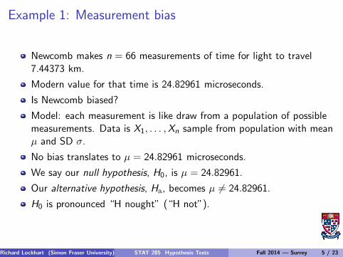
Newcomb makes n = 66 measurements of time for light to travel7.44373 km.

Modern value for that time is 24.82961 microseconds.

Is Newcomb biased?

Model: each measurement is like draw from a population of possiblemeasurements. Data is X1, . . . ,Xn sample from population with meanµ and SD σ.

No bias translates to µ = 24.82961 microseconds.

We say our null hypothesis, H0, is µ = 24.82961.

Our alternative hypothesis, Ha, becomes µ 6= 24.82961.

H0 is pronounced “H nought” (“H not”).


The test statistic

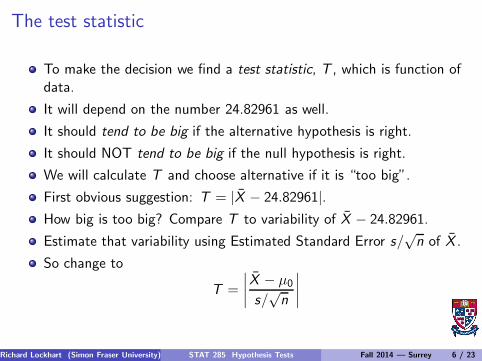
To make the decision we find a test statistic, T , which is function ofdata.

It will depend on the number 24.82961 as well.

It should tend to be big if the alternative hypothesis is right.

It should NOT tend to be big if the null hypothesis is right.

We will calculate T and choose alternative if it is “too big”.

First obvious suggestion: T = |X̄ − 24.82961|.How big is too big? Compare T to variability of X̄ − 24.82961.

Estimate that variability using Estimated Standard Error s/√n of X̄ .

So change to

T =

∣

∣

∣

∣

X̄ − µ0

s/√n

∣

∣

∣

∣


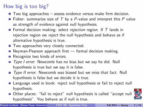
How big is too big?Two big approaches – assess evidence versus make firm decision.Fisher: summarize size of T by a P-value and interpret this P valueas strength of evidence against null hypothesis.Formal decision making: select rejection region. If T lands inrejection region we reject the null hypothesis and behave as ifalternative hypothesis is true.Two approaches very closely connected.Neyman-Pearson approach first — formal decision making.Recognize two kinds of errors.Type I error: Newcomb has no bias but we say he did. Nullhypothesis is true but we say it is false.Type II error: Newcomb was biased but we miss that fact. Nullhypothesis is false but we decide it is true.Language used in book: reject null hypothesis or fail to reject nullhypothesis.Other places: “fail to reject” null hypothesis is called “accept nullhypothesis”. You behave as if null is true.


Making a decision

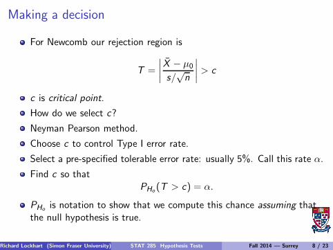
For Newcomb our rejection region is

T =

∣

∣

∣

∣

X̄ − µ0

s/√n

∣

∣

∣

∣

> c

c is critical point.

How do we select c?

Neyman Pearson method.

Choose c to control Type I error rate.

Select a pre-specified tolerable error rate: usually 5%. Call this rate α.

Find c so thatPHo

(T > c) = α.

PHois notation to show that we compute this chance assuming that

the null hypothesis is true.


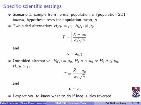
Specific scientific settings

Scenario 1: sample from normal population, σ (population SD)known, hypothesis tests for population mean, µ.

Two sided alternative: H0:µ = µ0, Ha:µ 6= µ0

T =

∣

∣

∣

∣

X̄ − µ0

σ/√n

∣

∣

∣

∣

andc = zα/2

One sided alternative. H0:µ = µ0, Ha:µ > µ0 or H0:µ ≤ µ0,Ha:µ > µ0.

T =X̄ − µ0

σ/√n

andc = zα

I expect you to know what to do if inequalities reversed.


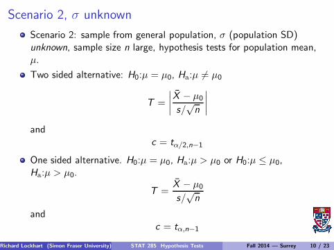
Scenario 2, σ unknown

Scenario 2: sample from general population, σ (population SD)unknown, sample size n large, hypothesis tests for population mean,µ.

Two sided alternative: H0:µ = µ0, Ha:µ 6= µ0

T =

∣

∣

∣

∣

X̄ − µ0

s/√n

∣

∣

∣

∣

andc = tα/2,n−1

One sided alternative. H0:µ = µ0, Ha:µ > µ0 or H0:µ ≤ µ0,Ha:µ > µ0.

T =X̄ − µ0

s/√n

andc = tα,n−1


Small samples

Scenario 3: sample from normal population, σ (population SD)unknown, sample size n anything, CI for population mean, µ.

Use same method as Scenario 2.

But now the method is exact.

Without the normal population assumption we are relying on the CLTand LLN and Slutsky’s theorem.


Hypothesis tests for proportions

Common scientific framework

Sequence of Bernoulli trials.

Number n fixed, p is “Success Probability” on each trial.

X is the number of successes.

Goal is a hypothesis test for proportions.

Method based on application of the Central Limit Theorem.

Same list of null / alternative choices: H0:p = p0 or H0:p ≤ p0

H0:p = p0 allows either 1 or 2 sided alternatives.


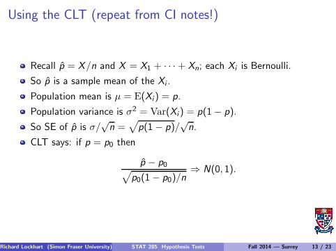
Using the CLT (repeat from CI notes!)

Recall p̂ = X/n and X = X1 + · · ·+ Xn; each Xi is Bernoulli.

So p̂ is a sample mean of the Xi .

Population mean is µ = E(Xi) = p.

Population variance is σ2 = Var(Xi ) = p(1− p).

So SE of p̂ is σ/√n =

√

p(1− p)/√n.

CLT says: if p = p0 then

p̂ − p0√

p0(1− p0)/n⇒ N(0, 1).


Using the CLT 2

Our test statistic is either

T =p̂ − p0

√

p0(1− p0)/n

for Ha:p > p0 or

T =

∣

∣

∣

∣

∣

p̂ − p0√

p0(1− p0)/n

∣

∣

∣

∣

∣

for Ha:p 6= p0

Critical value c iszα/2

for two-sided alternative orzα

for one-sided alternative.


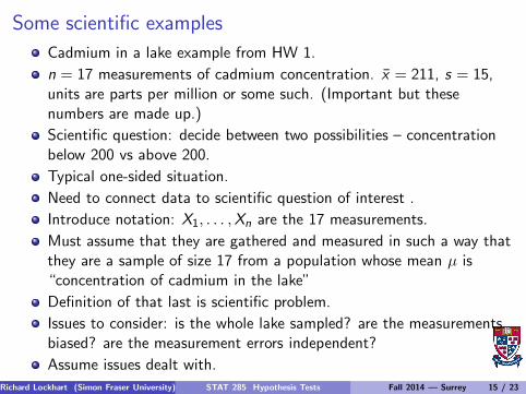
Some scientific examples

Cadmium in a lake example from HW 1.

n = 17 measurements of cadmium concentration. x̄ = 211, s = 15,units are parts per million or some such. (Important but thesenumbers are made up.)

Scientific question: decide between two possibilities – concentrationbelow 200 vs above 200.

Typical one-sided situation.

Need to connect data to scientific question of interest .

Introduce notation: X1, . . . ,Xn are the 17 measurements.

Must assume that they are gathered and measured in such a way thatthey are a sample of size 17 from a population whose mean µ is“concentration of cadmium in the lake”

Definition of that last is scientific problem.

Issues to consider: is the whole lake sampled? are the measurementsbiased? are the measurement errors independent?

Assume issues dealt with.


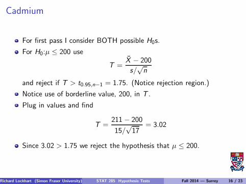
Cadmium

For first pass I consider BOTH possible H0s.

For H0:µ ≤ 200 use

T =X̄ − 200

s/√n

and reject if T > t0.95,n−1 = 1.75. (Notice rejection region.)

Notice use of borderline value, 200, in T .

Plug in values and find

T =211 − 200

15/√17

= 3.02

Since 3.02 > 1.75 we reject the hypothesis that µ ≤ 200.


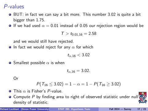
P-values

BUT: in fact we can say a bit more. This number 3.02 is quite a bitbigger than 1.75.

If we had used α = 0.01 instead of 0.05 our rejection region would be

T > t0.01,16 = 2.58

and we would still have rejected.

In fact we would reject for any α for which

tα,16 < 3.02

Smallest possible α is when

tα,16 = 3.02.

OrP(T16 ≤ 3.02) = 1− α = 1− P(T16 ≥ 3.02)

This α is Fisher’s P-value.

Compute P by finding area to right of observed statistic under nulldensity of statistic.


P-values

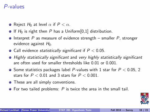
Reject H0 at level α if P < α.

If H0 is right then P has a Uniform[0,1] distribution.

Interpret P as measure of evidence strength – smaller P , strongerevidence against H0.

Call evidence statistically significant if P < 0.05.

Highly statistically significant and very highly statistically significant

are often used for smaller thresholds like 0.01 or 0.001.

Some statistics packages label P-values with 1 star for P < 0.05, 2stars for P < 0.01 and 3 stars for P < 0.001.

These are all simply conventions.

For two tailed problems: P is twice the area in the small tail.


Q 65 as an example

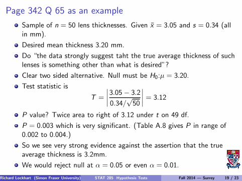
Sample of n = 50 lens thicknesses. Given x̄ = 3.05 and s = 0.34 (allin mm).

Desired mean thickness 3.20 mm.

Do “the data strongly suggest taht the true average thickness of suchlenses is something other than what is desired”?

Clear two sided alternative. Null must be H0:µ = 3.20.

Test statistic is

T =

∣

∣

∣

∣

3.05 − 3.2

0.34/√50

∣

∣

∣

∣

= 3.12

P value? Twice area to right of 3.12 under t on 49 df.

P = 0.003 which is very significant. (Table A.8 gives P in range of0.002 to 0.004.)

So we see very strong evidence against the assertion that the trueaverage thickness is 3.2mm.

We would reject null at α = 0.05 or even α = 0.01.


Error rates and sample size calculations

Type I error: incorrectly reject H0.

Type II error: incorrectly fail to reject H0.

Type I error rate is α; determined in advance.

Type II error rate is β – depends on what true parameter value is.

Can sometimes compute β = P(don’t reject) as a function.

Answer will depend on n.

Can then sometimes choose n to give suitable sample size.

But often n depends on unknown parameters like σ.

So we design for some hoped for value of σ.


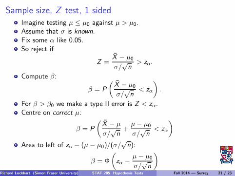
Sample size, Z test, 1 sidedImagine testing µ ≤ µ0 against µ > µ0.Assume that σ is known.Fix some α like 0.05.So reject if

Z =X̄ − µ0

σ/√n

> zα.

Compute β:

β = P

(

X̄ − µ0

σ/√n

< zα

)

.

For β > β0 we make a type II error is Z < zα.Centre on correct µ:

β = P

(

X̄ − µ

σ/√n+

µ− µ0

σ/√n

< zα

)

Area to left of zα − (µ− µ0)/(σ/√n):

β = Φ

(

zα − µ− µ0

σ/√n

)


Sample size calculation

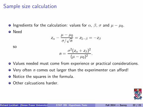
Ingredients for the calculation: values for α, β, σ and µ− µ0.

Need

zα − µ− µ0

σ/√n

= z1−β = −zβ

so

n =σ2(zα + zβ)

2

(µ− µ0)2.

Values needed must come from experience or practical considerations.

Very often n comes out larger than the experimenter can afford!

Notice the squares in the formula.

Other calcuations harder.


Sample sizes for other tests

Two sided tests: If the desired error rate β is reasonably small thenoften can use the one sized formula with zα/2 and zβ/2 to goodapproximation

Sometimes we are willing to specify (µ− µ0)/σ without necessarilyspecifying either σ or µ exactly.

Then use graphs in Table A.17 for small samples and formula abovefor large.

If you get a large sample size from the previous calculation then yourapproximation will be ok.

If you get a small sample size from the previous calculation use TableA.17.

For proportions. Remember σ = p(1− p) and use the previousformulas. See page 325 for details.

If n comes out small (which is very rarely the case) then you need tocompute β using the Binomial distribution, not a normal approx.


STAT 285 Hypothesis Tests - SFU

Documents

Transcript of STAT 285 Hypothesis Tests - SFU