Stat 13, Intro. to Statistical Methods for the Life and Health Sciences.

1.Whentousewhichformula.2.Multipletestingandpublicationbias.3.Twoquantitativevariables,correlation.4.Linearregression.

1

1.Whentousewhichformula.a.1samplenumericaldata,iid observations,wanta95%CIforµ.• Ifnislargeands isknown,use�̅� +/- 1.96s/√n.• Ifnissmall,drawsarenormal,ands isknown,use�̅� +/- 1.96s/√n.• Ifnissmall,drawsarenormal,ands isunknown,use�̅� +/- tmult s/√n.• Ifnislargeand s isunknown,tmult ~1.96,sowecanuse�̅� +/- 1.96s/√n.

n≥30isoftenconsideredlargeenoughtouse1.96.Inpractice,wetypicallydonotknowthedrawsarenormal,butifthedistributionlooksroughlysymmetricalwithoutenormousoutliers,thetformulamaybereasonable.

b.1samplebinarydata,iid observations,wanta95%CIforπ.

Viewthedataas0or1,sosamplepercentagep=�̅�, ands=√[p(1-p)],s = √[p(1-p)].

1.Whentousewhichformula.a.1samplenumericaldata,iid observations,wanta95%CIforµ.• Ifnislargeands isknown,use�̅� +/- 1.96s/√n.• Ifnissmall,drawsarenormal,ands isknown,use�̅� +/- 1.96s/√n.• Ifnissmall,draws~normal,ands isunknown,use�̅� +/- tmult s/√n.• Ifnislargeand s isunknown,tmult ~1.96,sowecanuse�̅� +/- 1.96s/√n.

b.1samplebinarydata,iid observations,wanta95%CIforπ.

Viewthedataas0or1,sosamplepercentagep=�̅�, ands=√[p(1-p)],s = √[p(1-p)].Ifnislargeandπisunknown,use�̅� +/- 1.96s/√n.

Herelargenmeans≥10ofeachtypeinthesample.

Whatifnissmallandthedrawsarenotnormal?Thatisasituationoutsidethescopeofthiscourse,butsometechniqueshavebeendeveloped,suchasthebootstrap,whicharesometimesusefulinthesesituations.

1.Whentousewhichformula.c.Numericaldatafrom2samples,iid observations,wanta95%CIforµ1 - µ2.

Ifnislargeands isunknown,use𝑥1( - �̅�2+/- 1.96)*+

,*+ )++

,+

�.

Aswithonesample,ifs1 isknown,replaces1 withs1,andthesamefors2.Andaswithonesample,ifs1 ands2 areunknown,thesamplesizesaresmall,andthedistributionsareroughlynormal,thenusetmult insteadof1.96.Ifthesamplesizesaresmall,thedistributionsarenormal,ands1ands2 areknown,thenuse1.96.

d.Binarydatafrom2samples,iid observations,wanta95%CIforπ1 - π2.sameasincabove,withp1 = 𝑥1( ,s1 =√[p1(1-p1)],s1 = √[p1(1-p1)].Largeforbinarydatameanssamplehas≥10ofeachtype.

1.Whentousewhichformula.e.Matchedpairsdata,iid observations,wanta95%CIforµ.Lookatdifferences(scorewithtreatmentminusscorewithcontrol)andtreatdifferencesasordinarynumericaldataaccordingtopartsaorb.• Ifnislargeands isknown,use�̅� +/- 1.96s/√n.• Ifnissmall,drawsarenormal,ands isknown,use�̅� +/- 1.96s/√n.• Ifnissmall,drawsarenormal,ands isunknown,use�̅� +/- tmult s/√n.• Ifnislargeand s isunknown,tmult ~1.96,sowecanuse�̅� +/- 1.96s/√n.

n≥30isoftenconsideredlargeenoughtouse1.96.Inpractice,wetypicallydonotknowthedrawsarenormal,butifthedistributionlooksroughlysymmetricalwithoutenormousoutliers,thetformulamaybereasonable.

2.Multipletestingandpublicationbias.Ap-valueistheprobability,assumingthenullhypothesisofnorelationshipistrue,thatyouwillseeadifferenceasextremeas,ormoreextremethan,youobserved.So,5%ofthetimeyouarelookingatunrelatedthings,youwillfindastatisticallysignificantrelationship.Thisunderscorestheneedforfollowup confirmationstudies.Iftestingmanyexplanatoryvariablessimultaneously,itcanbecomeverylikelytofindsomethingsignificantevenifnothingisactuallyrelatedtotheresponsevariable.

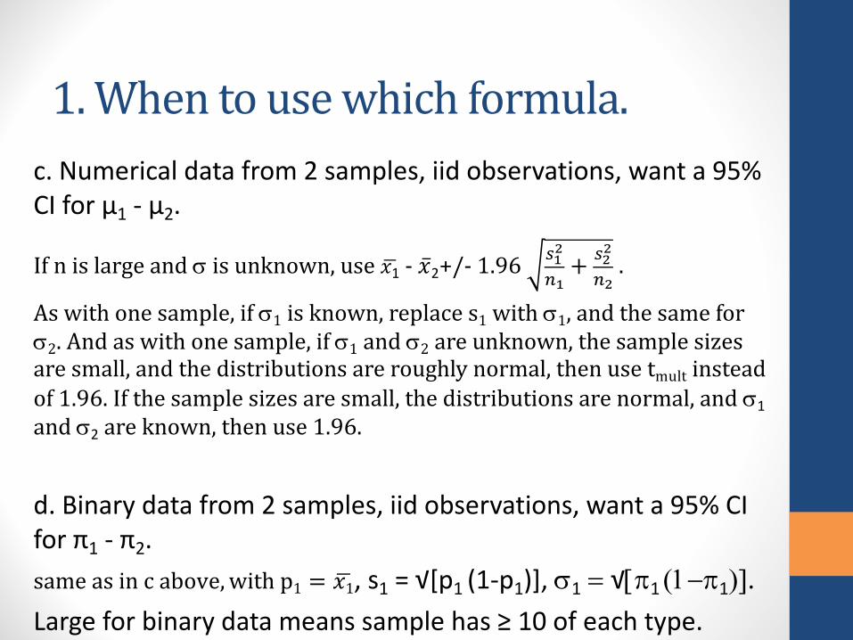
Multipletestingandpublicationbias.*Forexample,ifthesignificancelevelis5%,thenfor100testswhereallnullhypothesesaretrue,theexpectednumberofincorrectrejections(TypeIerrors)is5.Ifthetestsareindependent,theprobabilityofatleastoneTypeIerrorwouldbe99.4%.*Toaddressthisproblem,scientistssometimeschangethesignificancelevelsothat,underthenullhypothesisthatnoneoftheexplanatoryvariablesisrelatedtotheresponsevariable,theprobabilityofrejectingany ofthemis5%.*OnewayistouseBonferroni'scorrection:withmexplanatoryvariables,usesignificancelevel5%/m.P(atleast1TypeIerror)willbe≤ m(5%/m)=5%.

P(TypeIerroronexplanatory1)=5%/m.P(TypeIerroronexplanatory2)=5%/m.P(Type1erroronatleastoneexplanatory)≤P(erroron1)+P(erroron2)+...+P(erroronm) =mx5%/m.

Multipletestingandpublicationbias.

Imagineascenariowhereadrugistestedmanytimestoseeifitreducestheincidenceofsomeresponsevariable.Ifthedrugistestes100timesby100differentresearchers,theresultswillbestat.sig.about5times.Ifonlythestat.sig.resultsarepublished,thenthepublishedrecordwillbeverymisleading.

Multipletestingandpublicationbias.AdrugcalledReboxetine madebyPfizerwasapprovedasatreatmentfordepressioninEuropeandtheUKin2001,basedonpositivetrials.Ameta-analysisin2010foundthatitwasnotonlyineffectivebutalsopotentiallyharmful.Thereportfoundthat74%ofthedataonpatientswhotookpartinthetrialsofReboxetine werenotpublishedbecausethefindingswerenegative.Publisheddataaboutreboxetine overestimateditsbenefitsandunderestimateditsharm.Asubsequent2011analysisindicatedReboxetinemightbeeffectiveforseveredepressionthough.

3.TwoQuantitativeVariablesChapter10

TwoQuantitativeVariables:ScatterplotsandCorrelationSection10.1

ScatterplotsandCorrelation

Time 30 41 41 43 47 48 51 54 54 56 56 56 57 58

Score 100 84 94 90 88 99 85 84 94 100 65 64 65 89

Time 58 60 61 61 62 63 64 66 66 69 72 78 79

Score 83 85 86 92 74 73 75 53 91 85 62 68 72

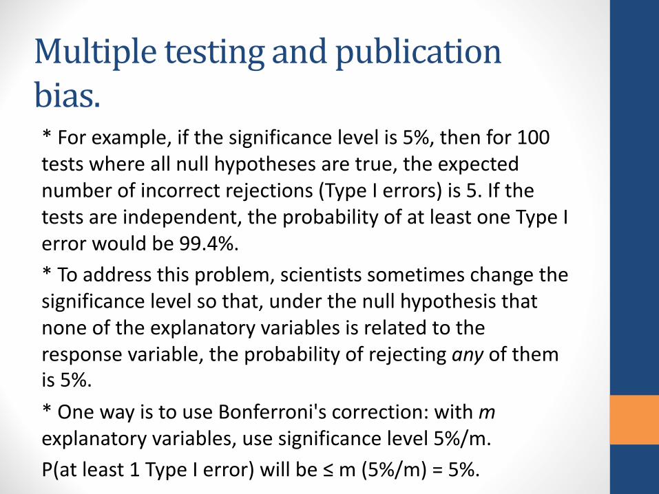
Supposewecollecteddataontherelationshipbetweenthetimeittakesastudenttotakeatestandtheresultingscore.

Scatterplot

Putexplanatoryvariableonthehorizontalaxis.

Putresponsevariableontheverticalaxis.

DescribingScatterplots•Whenwedescribedatainascatterplot,wedescribethe• Direction(positiveornegative)• Form(linearornot)• Strength(strong-moderate-weak,wewillletcorrelationhelpusdecide)• UnusualObservations• Howwouldyoudescribethetimeandtestscatterplot?

Correlation• Correlationmeasuresthestrengthanddirectionofalinear associationbetweentwoquantitative variables.• Correlationisanumberbetween-1and1.• Withpositivecorrelationonevariableincreases,onaverage,astheotherincreases.• Withnegativecorrelationonevariabledecreases,onaverage,astheotherincreases.• Thecloseritistoeither-1or1thecloserthepointsfittoaline.• Thecorrelationforthetestdatais-0.56.

CorrelationGuidelinesCorrelationValue Strengthof

AssociationWhatthismeans

0.7to1.0 Strong Thepointswillappeartobenearlyastraightline

0.3to0.7 Moderate Whenlookingatthegraphtheincreasing/decreasingpatternwillbeclear,but thereisconsiderablescatter.

0.1to0.3 Weak Withsomeeffortyouwillbeabletoseeaslightlyincreasing/decreasingpattern

0to0.1 None Nodiscernibleincreasing/decreasingpattern

Same StrengthResultswithNegativeCorrelations

BacktothetestdataActuallythelastthreepeopletofinishthetesthadscoresof93,93,and97.

Whatdoesthisdotothecorrelation?

InfluentialObservations• Thecorrelationchangedfrom-0.56(afairlymoderatenegativecorrelation)to-0.12(aweaknegativecorrelation).• Pointsthatarefartotheleftorrightandnotintheoveralldirectionofthescatterplotcangreatlychangethecorrelation.(influentialobservations)

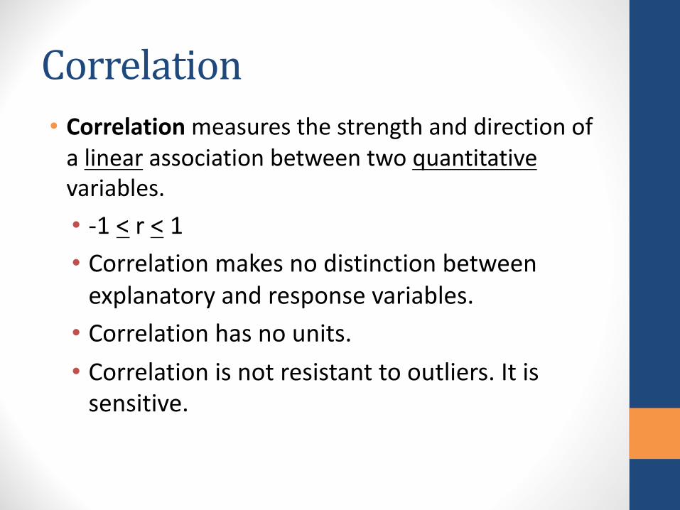
Correlation• Correlationmeasuresthestrengthanddirectionofalinear associationbetweentwoquantitativevariables.• -1< r< 1• Correlationmakesnodistinctionbetweenexplanatoryandresponsevariables.• Correlationhasnounits.• Correlationisnotresistanttooutliers.Itissensitive.

LearningObjectivesforSection10.1• Summarizethecharacteristicsofascatterplotbydescribingitsdirection,form,strengthandwhetherthereareanyunusualobservations.• Recognizethatthecorrelationcoefficientisappropriateonlyforsummarizingthestrengthanddirectionofascatterplotthathaslinearform.• Recognizethatascatterplotistheappropriategraphfordisplayingtherelationshipbetweentwoquantitativevariablesandcreateascatterplotfromrawdata.• Recognizethatacorrelationcoefficientof0meansthereisnolinearassociationbetweenthetwovariablesandthatacorrelationcoefficientof-1or1meansthatthescatterplotisexactlyastraightline.• Understandthatthecorrelationcoefficientisinfluencedbyextremeobservations.

InferencefortheCorrelationCoefficient:Simulation-BasedApproachSection10.2

Wewilllookatasmallsampleexampletoseeifbodytemperatureisassociatedwithheartrate.

TemperatureandHeartRateHypotheses

• Null:Thereisnoassociationbetweenheartrateandbodytemperature.(ρ=0)• Alternative:Thereisapositivelinearassociationbetweenheartrateandbodytemperature.(ρ>0)

ρ=rho

InferenceforCorrelationwithSimulation(Section10.2)

1.Computetheobservedstatistic.(Correlation)2.Scrambletheresponsevariable,computethesimulatedstatistic,andrepeatthisprocessmanytimes.

3.Rejectthenullhypothesisiftheobservedstatisticisinthetailofthenulldistribution.

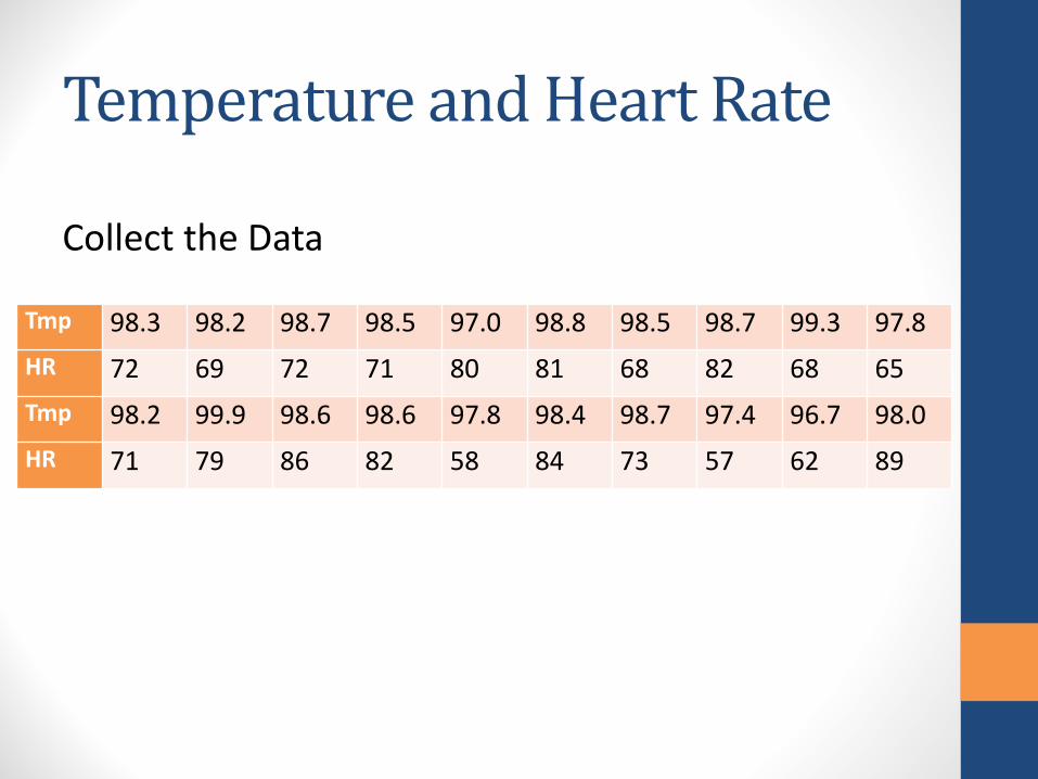
TemperatureandHeartRate

Tmp 98.3 98.2 98.7 98.5 97.0 98.8 98.5 98.7 99.3 97.8HR 72 69 72 71 80 81 68 82 68 65Tmp 98.2 99.9 98.6 98.6 97.8 98.4 98.7 97.4 96.7 98.0HR 71 79 86 82 58 84 73 57 62 89

CollecttheData

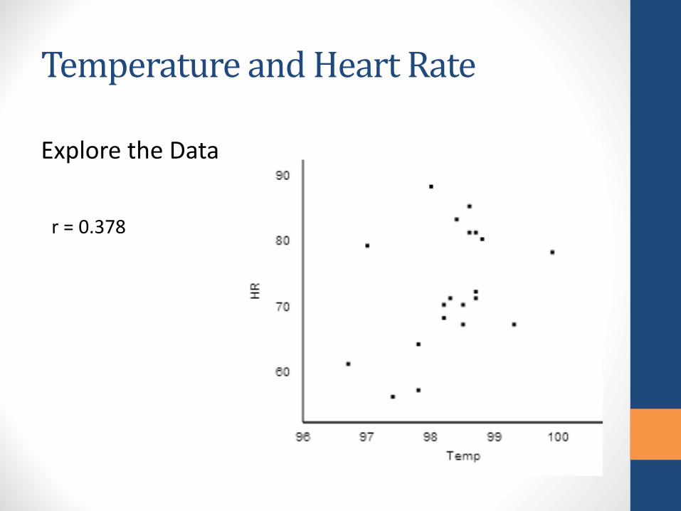
TemperatureandHeartRate

r=0.378

ExploretheData

TemperatureandHeartRate• Iftherewasnoassociationbetweenheartrateandbodytemperature,whatistheprobabilitywewouldgetacorrelationashighas0.378justbychance?

• Ifthereisnoassociation,wecanbreakapartthetemperaturesandtheircorrespondingheartrates.Wewilldothisbyshufflingoneofthevariables.

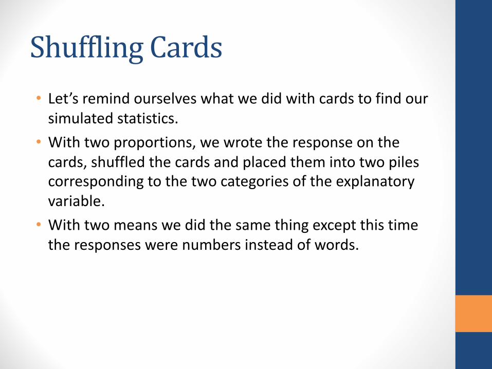
ShufflingCards• Let’sremindourselveswhatwedidwithcardstofindoursimulatedstatistics.• Withtwoproportions,wewrotetheresponseonthecards,shuffledthecardsandplacedthemintotwopilescorrespondingtothetwocategoriesoftheexplanatoryvariable.• Withtwomeanswedidthesamethingexceptthistimetheresponseswerenumbersinsteadofwords.

20.0% Improvers

66.7% Improvers

DolphinTherapyControlNon-

improver

Improver

Improver

Improver

Improver

Improver

Improver

Improver

ImproverImprover

Improver

Improver

Improver

ImproverNon-improver

Non-improver

Non-improver

Non-improver

Non-improver

Non-improver

Non-improver

Non-improver

Non-improver

Non-improver

Non-improver

Non-improver

Non-improver

Non-improver

Non-improver

Non-improver

40.0% Improvers

46.7% Improvers0.400 – 0.467 = -0.067

Difference in Simulated Proportions

mean = 3.90mean = 19.82

Music Nomusic

14.5

25.2

11.6

12.6

18.6

12.1

30.534.5

-7.0

45.6 10.0

9.6

-10.7

7.2-14.7

21.3

2.2

4.5

-10.7

21.8

2.4

mean = 6.38 mean = 16.126.38 – 16.12 = -9.74

Difference in Simulated Means

ShufflingCards• Nowhowwillthisshufflingbedifferentwhenboththeresponseandtheexplanatoryvariablearequantitative?• Wecan’tputthingsintwopilesanymore.• Westillshufflevaluesoftheresponsevariable,butthistimeplacethemnexttotwovaluesoftheexplanatoryvariable.

98.3° 98.2° 97.7° 98.5° 97.0° 98.8° 98.5° 98.7° 99.3° 97.8°

98.2° 99.9° 98.6° 98.6° 97.8° 98.4° 98.7° 97.4° 96.7° 98.0°

r = 0.378

6972 8180 82687172

r = 0.073

Simulated Correlations

Body Temperature and Heart Rate

68 65

7971 8458 57738286 62 89

MoreSimulations0.054

-0.253 -0.3450.062 0.259

0.339

0.447-0.008

-0.229

-0.0290.059 -0.006

-0.034

-0.327 0.1000.067

0.212

0.097

0.447

0.034

0.167

0.3290.020

-0.042

0.232

0.2000.314

Only one simulated statistic out of 30 was as large or larger than our observed correlation of 0.378, hence our p-value for this null distribution is 1/30 ≈ 0.03.

Simulated Correlations 0.378

TemperatureandHeartRate• Wecanlookattheoutputof1000shuffleswithadistributionof1000simulatedcorrelations.

TemperatureandHeartRate• Noticeournulldistributioniscenteredat0andsomewhatsymmetric.• Wefoundthat530/10000timeswehadasimulatedcorrelationgreaterthanorequalto0.378.

TemperatureandHeartRate• Withap-valueof0.053=5.3%,wealmostbutdonotquitehavestatisticalsignificance.Thisismoderateevidenceofapositivelinearassociationbetweenbodytemperatureandheartrate.Perhapsalargersamplewouldgiveasmallerp-value.

4.LeastSquaresRegressionSection10.3

Introduction• Ifwedecideanassociationislinear,itishelpfultodevelopamathematicalmodelofthatassociation.• Helpsmakepredictionsabouttheresponsevariable.• Theleast-squaresregressionline isthemostcommonwayofdoingthis.

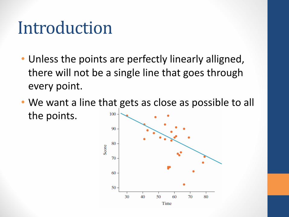
Introduction• Unlessthepointsareperfectlylinearlyalligned,therewillnotbeasinglelinethatgoesthrougheverypoint.• Wewantalinethatgetsascloseaspossibletoallthepoints.

Introduction• Wewantalinethatminimizestheverticaldistancesbetweenthelineandthepoints• Thesedistancesarecalledresiduals.• Thelinewewillfindactuallyminimizesthesumofthesquaresoftheresiduals.• Thisiscalledaleast-squaresregressionline.

AreDinnerPlatesGettingLarger?Example10.3

GrowingPlates?• TherearemanyrecentarticlesandTVreportsabouttheobesityproblem.• Onereasonsomehavegivenisthatthesizeofdinnerplatesareincreasing.• Aretheseblackcirclesthesamesize,orisonelargerthantheother?

GrowingPlates?• Theyappeartobethesamesizeformany,buttheoneontherightisabout20%largerthantheleft.

• Thissuggeststhatpeoplewillputmorefoodonlargerdinnerplateswithoutknowingit.

• Thereisnameforthisphenomenon:Delboeufillusion

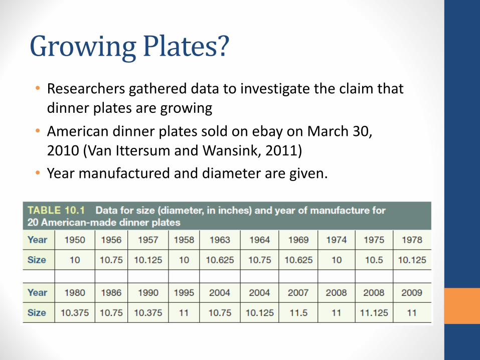
GrowingPlates?• Researchersgathereddatatoinvestigatetheclaimthatdinnerplatesaregrowing• Americandinnerplatessoldonebay onMarch30,2010(VanIttersum andWansink,2011)• Yearmanufacturedanddiameteraregiven.

GrowingPlates?• Bothyear(explanatoryvariable)anddiameterininches(responsevariable)arequantitative.• Eachdotrepresentsoneplateinthisscatterplot.• Describetheassociationhere.

GrowingPlates?• Theassociationappearstoberoughlylinear• Theleastsquaresregressionlineisadded• Howcanwedescribethisline?

RegressionLineTheregressionequationis𝑦< = 𝑎 + 𝑏𝑥:• a isthey-intercept• b istheslope• x isavalueoftheexplanatoryvariable• ŷ isthepredictedvaluefortheresponsevariable

• Foraspecificvalueofx,thecorrespondingdistancey − 𝑦< (oractual– predicted)isaresidual

RegressionLine• Theleastsquareslineforthedinnerplatedatais𝑦< = −14.8 + 0.0128𝑥• OrdiameterH = −14.8 + 0.0128(year)• Thisallowsustopredictplatediameterforaparticularyear.

Slope𝑦< = −14.8 + 0.0128𝑥

• Whatisthepredicteddiameterforaplatemanufacturedin2000?• -14.8+0.0128(2000)=10.8in.

• Whatisthepredicteddiameterforaplatemanufacturedin2001?• -14.8+0.0128(2001)=10.8128in.

• Howdoesthiscomparetoourpredictionfortheyear2000?• 0.0128larger

• Slopeb =0.0128meansthatdiametersarepredictedtoincreaseby0.0128inchesperyearonaverage

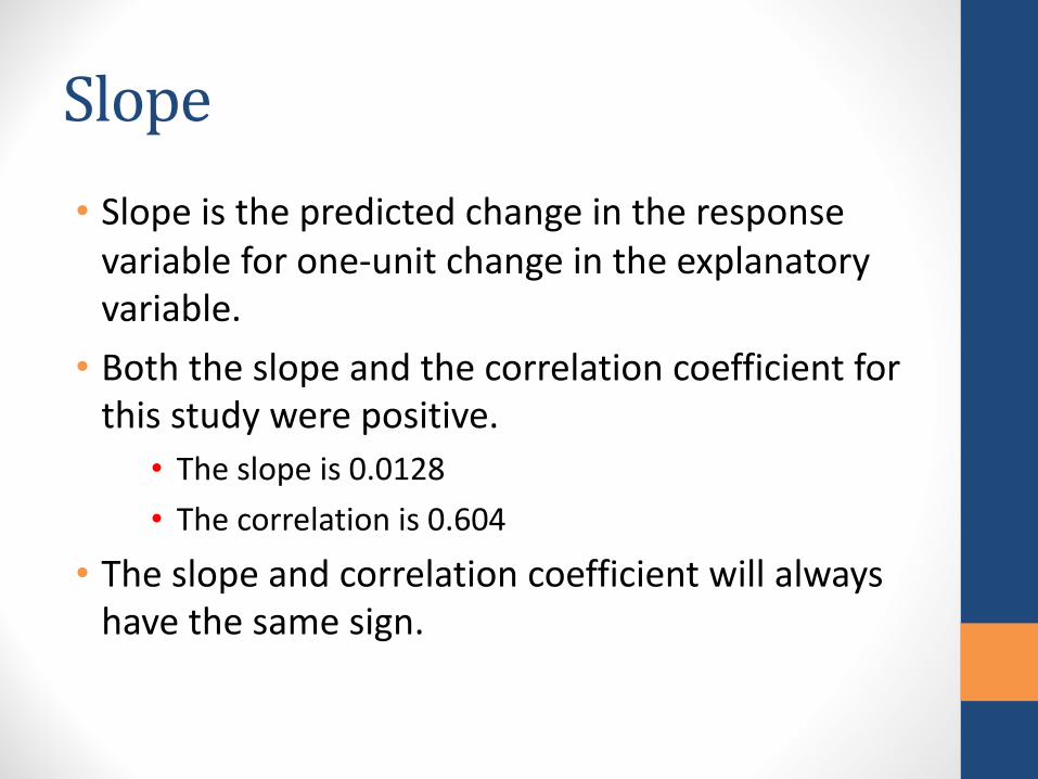
Slope• Slopeisthepredictedchangeintheresponsevariableforone-unitchangeintheexplanatoryvariable.• Boththeslopeandthecorrelationcoefficientforthisstudywerepositive.• Theslopeis0.0128• Thecorrelationis0.604

• Theslopeandcorrelationcoefficientwillalwayshavethesamesign.

y-intercept• They-interceptiswheretheregressionlinecrossesthey-axisorthepredictedresponsewhentheexplanatoryvariableequals0.• Wehaday-interceptof-14.8inthedinnerplateequation.Whatdoesthistellusaboutourdinnerplateexample?• Dinnerplatesinyear0were-14.8inches.

• Howcanitbenegative?• Theequationworkswellwithintherangeofvaluesgivenfortheexplanatoryvariable,butfailsoutsidethatrange.

• Ourequationshouldonlybeusedtopredictthesizeofdinnerplatesfromabout1950to2010.

Extrapolation• Predictingvaluesfortheresponsevariableforvaluesoftheexplanatoryvariablethatareoutsideoftherangeoftheoriginaldataiscalledextrapolation.

CoefficientofDetermination

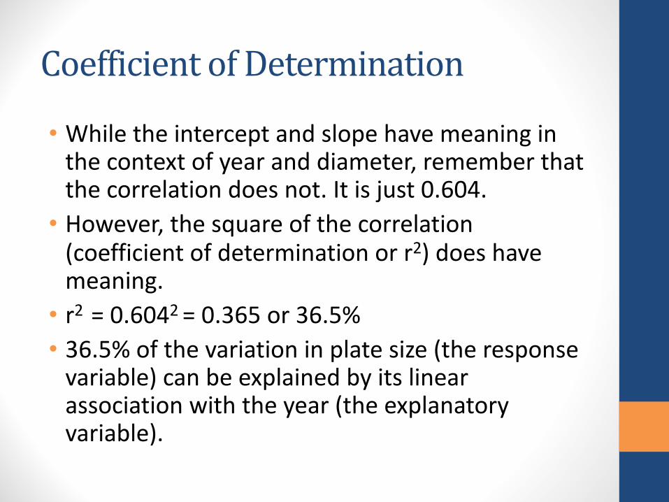
• Whiletheinterceptandslopehavemeaninginthecontextofyearanddiameter,rememberthatthecorrelationdoesnot.Itisjust0.604.• However,thesquareofthecorrelation(coefficientofdeterminationorr2)doeshavemeaning.• r2 =0.6042=0.365or36.5%• 36.5%ofthevariationinplatesize(theresponsevariable)canbeexplainedbyitslinearassociationwiththeyear(theexplanatoryvariable).

LearningObjectivesforSection10.3• Understandthatonewayascatterplotcanbesummarizedisbyfittingthebest-fit(leastsquaresregression)line.• Beabletointerpretboththeslopeandinterceptofabest-fitlineinthecontextofthetwovariablesonthescatterplot.• Findthepredictedvalueoftheresponsevariableforagivenvalueoftheexplanatoryvariable.• Understandtheconceptofresidualandfindandinterprettheresidualforanobservationalunitgiventherawdataandtheequationofthebestfit(regression)line.• Understandtherelationshipbetweenresidualsandstrengthofassociationandthatthebest-fit(regression)linethisminimizesthesumofthesquaredresiduals.

LearningObjectivesforSection10.3• Findandinterpretthecoefficientofdetermination(r2)asthesquaredcorrelationandasthepercentoftotalvariationintheresponsevariablethatisaccountedforbythelinearassociationwiththeexplanatoryvariable.• Understandthatextrapolationiswhenaregressionlineisusedtopredictvaluesoutsideoftherangeofobservedvaluesfortheexplanatoryvariable.• Understandthatwhenslope=0meansnoassociation,slope<0meansnegativeassociation,slope>0meanspositiveassociation,andthatthesignoftheslopewillbethesameasthesignofthecorrelationcoefficient.• Understandthatinfluentialpointscansubstantiallychangetheequationofthebest-fitline.