Startup Search Costs

Startup Search Costs*

David P. Byrne† Nicolas de Roos‡

October 29, 2018

Abstract

Workhorse economic models used for studying the market impacts of search frictions as-

sume constant search costs: individuals pay the same cost to obtain price information each

time they search. This paper provides evidence on a new form of search costs: startup costs.

Exploiting a natural experiment in retail gasoline, we document how a temporary, large ex-

ogenous shock to consumers’ search incentives leads to a substantial, permanent increase

in price search. A standard search model fails to explain such history-dependence in search,

while it follows directly from a model with a one-time up-front cost to start searching.

JEL Classification: D83, L81

Keywords: Search, Price Dispersion, Price War, Retail Gasoline

*We recommend viewing this article in color. We thank Simon Loertscher, Eeva Mauring, Wanda Mimra, JoseMoraga-Gonzalez, Philipp Schmidt-Dengler, Paul Scott, Matthew Shum, Michelle Sovinsky, Tom Wilkening, NanYang, and seminar participants from the University of Melbourne, University of Groningen, University of Vienna,ESMT Berlin, Mines ParisTech, University of Adelaide, University of Technology Sydney, NYU Stern School ofBusiness, 2016 Asia-Pacific IO Conference, 2017 Monash IO Workshop, and 2018 Tinbergen Institute EmpiricalIO Workshop for helpful comments. The views expressed herein are solely those of the authors. Any errors oromissions are our own.

†Department of Economics, The University of Melbourne, Level 4 111 Barry Street, VIC 3010, Australia, e-mail:[email protected].

‡School of Economics, The University of Sydney, Merewether Building H04, NSW 2006, Australia, e-mail: [email protected].

1 Introduction

To purchase a flight, find a nice restaurant, or fill up one’s gas tank, consumers must set aside

time and effort to search for the most suitable or affordable option. According to the theory

of search, the trade–off between these search costs and the expected benefits from searching

determines the set of prices and products considered by a consumer, and firms’ market power.1

In applications of search models that study this trade-off, parsimony is important for tractibil-

ity, and it is commonly assumed that the cost of search is independent of a consumer’s past

experience searching for prices and products.

In this paper, we provide evidence on a new form of search costs that we call startup search

costs. These costs represent a one-time, up-front cost and individual incurs the first time they

engage in search behavior. After a startup search cost is sunk, their cost of search for future

purchases is reduced. To establish the existence of such startup search costs, we leverage a

unique dataset and natural experiment in retail gasoline.

Section 2 describes the dataset. The data come from an urban gasoline market that has an

online price clearinghouse which consumers can use to become informed about the retail price

distribution across stations day-to-day. We have access to the universe of station-level gasoline

prices from 2014-2016, which we match to daily website usage from the price clearinghouse.

Our ability to perfectly measure price levels and dispersion, and directly measure market-level

search behavior from a price clearinghouse in a homogeneous product market, makes this con-

text particularly well–suited for studying the dynamics of search and price dispersion.2

In Section 3, we describe the natural experiment which occurs mid-sample. We then ex-

ploit the experiment to identify the causal impact of a temporary, large exogenous shock to

consumers’ search incentives on search intensity in the short and long-run.

The natural experiment stems from a price war that disrupts a stable coordinated pricing

equilibrium. In a separate study, Byrne and de Roos (2018), we document five years of stable

and highly coordinated pricing in the market from March 2010 to April 2015, which is consistent

with tacit collusion. However, in May 2015, a price war occurs and price coordination breaks

down. During a three-week conflict period, retail price dispersion spikes and the daily gains

from search grow by 100% relative to their pre-war levels. Firms eventually resolve the war and

return to stable coordinated pricing, and price dispersion and search incentives return to their

baseline (pre-war) levels. Based on pre-war retail price and search dynamics in our dataset,

1Baye, Morgan, and Scholten (2006) overview an extensive and influential literature on search models, whichdate back to Stigler (1961).

2See, for example, de Los Santos, Hortascu, and Wildenbeest (2012) and Koulayev (2014) for analyses of searchmodels using web search data. See Eckert (2013) for an overview of an extensive literature on search and pricedispersion in retail gasoline.

1

and anecdotal evidence of a retail ownership change that precipitated the war, we argue that

the price war is exogenous to search behavior on the price clearinghouse.

We study search intensity on the price clearinghouse one year before and after this tempo-

rary shock to price dispersion and search incentives. Our main empirical result is that daily

search intensity permanently rises by 70% following the shock. We show that this rise in search

intensity comes from an increase in the number of unique searchers using the clearinghouse,

and not an increase in average search intensity among previous searchers. This finding of

history-dependence in search behavior points to new consumers experimenting with the clear-

inghouse for a first time in response to the substantial price uncertainty created by the price

war. Having tried it once, consumers continue to use the clearinghouse thereafter, even after

search incentives return to pre-war levels.

Section 4 moves beyond these reduced-form empirics and formalizes our notion of startup

search costs, estimates their magnitude, and shows how ignoring them leads to model misspec-

ification. Specifically, we develop and estimate a non-sequential search model that decom-

poses search costs into a startup and a recurrent component.3 Exploiting the natural experi-

ment, we estimate the relative magnitudes of startup search costs and recurrent search costs.

Our simple search model rationalizes the permanent rise in search intensity from a temporary

shock to search incentives. By contrast, a standard non-sequential search model is unable to

rationalize the persistent post-war increase in search that we find.

We conclude in Section 5. Our findings suggest that the omission of startup search costs

leads to qualitatively different inferences regarding search behavior. Moreover, our study il-

lustrates the challenges faced by policymakers when designing tools to enhance price trans-

parency when consumers face startup search costs: the price clearinghouse we study had been

in existence for 15 years by May 2015, more than 90% of the market were aware of its existence,

yet the price war shock still led to a 70% rise in the volume of search. Finally, we highlight av-

enues for future research. While we provide evidence on the existence of startup search costs

and measure their magnitude, further work is required to elicit their microeconomic founda-

tions.4 We close by discussing deeper possible mechanisms for the novel history-dependent

search behavior that we uncover.3Under non-sequential search, the entire vector of prices is revealed to a consumer that incurs a search cost.

This matches the market environment in which a comprehensive price clearinghouse operates; see Ellison (2016).4In this way, our startup search cost estimates are reduced forms like previous search cost estimates based on

sequential and non-sequential search models (e.g., Hong and Shum, 2006; de Los Santos et al., 2012; Koulayev,2014). Only recently have studies emerged that identify deeper microfoundations of recurrent search costs includ-ing spatial frictions (Pennerstorfer et al., 2017; Startz, 2018; Buchholz, 2018), salience and price obfuscation (Blakeet al., 2018), the value of time spent searching (Seiler and Pinna, 2017), and cognition (Crawford et al., 2013).

2

Figure 1: Fuelwatch Price Clearinghouse

2 Context and data

Our research context is Perth, Australia, a city with approximately 2 million people. Perth, like

many urban gasoline markets worldwide, has a concentrated retail gasoline market. Four major

firms dominate the market: BP, Caltex, Coles and Woolworths. The former two firms are verti-

cally integrated oil majors, while the latter two firms are major supermarket chains that also sell

gasoline. All four firms either directly or indirectly control retail prices day-to-day at their large

station networks. Combined, their station networks account for approximately 75% of stations

in the market. All other stations are operated by independent retailers.

A key aspect of the market is a price transparency program called Fuelwatch. The program

was introduced on January 3, 2001 by Western Australia’s state government. By law, before 2pm

each day firms must submit CSV files to the state government that contain tomorrow’s station-

level retail prices. The next day at 6am when stations open, they are required to post the prices

that were submitted at 2pm the previous day. Prices are then fixed for 24 hours. From our

conversations with the government, compliance with the program is near perfect.

With the Fuelwach price data, before 2pm each day the government posts online today’s

prices for all stations in the market. This helps customers engage in cross–sectional price search.

After a data verification check, at 2:30pm the government further posts tomorrow’s price for ev-

ery station in the market. This helps customers engage in inter–temporal price search. Figure 1

3

Table 1: Summary Statistics

Obs. Mean Std. Dev Min Max

Price dataStation Retail Price 146931 128.64 13.67 92.9 169Market Terminal Gate Price 731 118.3 12.6 95.8 147.0Station Retail Margin 146931 10.3 6.8 -17.0 35.7

Search dataDaily website visits 731 19699 6691 8243 53517Monthly unique website visitors 24 208184 47767 129630 276737

Notes: Sample period is July 1, 2014 to June 30, 2016.

depicts the Fuelwatch price clearinghouse at www.fuelwatch.gov.au. Survey evidence from the

Western Australian Government indicates that more than 90% of Perth households are aware of

the Fuelwatch price clearinghouse.5

2.1 Data

The price clearinghouse generates a uniquely rich dataset for studying retail price search and

price dispersion. From the clearinghouse, we have access to the universe of retail prices from

2001 to present day. This allows us to perfectly measure daily price levels and dispersion. We

match these price data to the daily terminal gate price (TGP) for gasoline, which is the local

spot price for wholesale gasoline. These spot prices include a margin for upstream suppliers

of gasoline. The difference between the retail price and TGP provides an estimate of the retail

margin. It is an appropriate estimate for studying the evolution of margins over time because

the TGP is the main time–varying component of stations’ wholesale fuel costs.6

Moreover, the state government provided us access to daily website usage data from the Fu-

elwatch website. More specifically, we were provided daily data on the total number of website

hits on the Fuelwatch website, and the total number of unique visitors to the Fuelwatch website

month–to–month. These search data, combined with the universe of station–level price data,

permit a direct examination of how retail search behavior responds to changes in price levels

and dispersion at the market level over time.7

5For example, in 2008 the Deputy Prices Commissioner of the Western Australian Department of Consumerand Employment Protection stated that “The last survey we did showed that 94 per cent of people had heard ofFuelWatch.” See Commonwealth, Parliamentary Debates, Senate Standing Committee on Economics, 16 July 2008,(Mr. Rayner), p. E 5.

6Other time–invariant parts of marginal costs include quantity discounts, shipping costs, wharfage fees, andinsurance costs.

7Daily data on the total number of unique visitors is unavailable due to data privacy concerns from the stategovernment. Similarly, daily data on website hits at the individual level or by disaggregated census blocks are not

4

Our sample period spans two-years, from July 1, 2014 to June 30, 2016. Over this period,

average station-level retail prices and margins in terms of cents per liter (cpl) are 128.6 cpl and

10.3 cpl, respectively. The average number of Fuelwatch website visits each day is 19699, and

there are 208184 unique visitors to the website each month on average. Table 1 presents sum-

mary statistics from our dataset.

2.2 Price cycles and search cycles

Figure 2 depicts cyclical patterns in retail price levels, price dispersion, and search that persist

over the entire sample period. Panel A, which plots average daily retail prices by retailer and

the daily TGP, highlights cycles in price levels. Over the time period shown in the figure, every

Thursday, retail prices jump by approximately 10% of the average market price. Between price

jumps, most retailers cut prices by 2 cpl each day until the next price jump day occurs. Intertem-

poral search incentives are therefore heightened on Wednesdays in anticipation of Thursday

price jumps.

Panel B plots corresponding daily market price dispersion, as measured by the daily stan-

dard deviation of retail prices across stations. For reference, we overlay daily price dispersion

with the price cycles from panel A in greyscale. The figure highlights spikes in price dispersion

on Thursdays, as the average of the standard deviation of retail prices rises from 4.97 at the bot-

tom of the cycle, to 6.77 cpl at the top of the cycle. This large rise in price dispersion reflects a

noisy coordination process as market prices transition from the bottom to the top of the cycle.

Cross–sectional search incentives thus tend to rise substantially on Thursdays.

Panel C of Figure 2 plots daily search intensity on the Fuelwatch website, as measured by

the number of website hits from computers and mobile devices. Like prices, search exhibits

cycles, whereby search intensity jumps on Wednesdays and Thursdays. On the day before and

day of price jumps, on average the website receives 27049 and 19531 visits, respectively. On

all other days, the website on average receives 18263 visits. In sum, search intensity rises with

cross–sectional and inter–temporal search incentives just before and during price jumps.

3 Dynamics of price dispersion and search

In this section, we examine the coevolution of retail prices and search over the entire two–year

sample period. We document the break out of a price war among the retailers who were previ-

ously coordinating on the timing and magnitude of price jumps and cuts. We describe the im-

pact of the price war on price levels, dispersion, and margins. We then show that daily search in-

available because of privacy concerns.

5

Figure 2: Price and Search Cycles Cycles

Panel A: Daily Retail Price Levels

130

140

150

160

170

Aver

age

Ret

ail P

rice,

TG

P

01jul2014 01aug2014 01sep2014 01oct2014Date

BP Caltex Woolworths Coles Gull TGP

Panel B: Daily Retail Price Dispersion

34

56

78

Std.

Dev

. of P

rices

Acr

oss

Stat

ions

130

140

150

160

170

Aver

age

Ret

ail P

rice,

TG

P


Daily Price Std. Dev.Across Stations

Panel C: Daily Number of Website Visits

5000

1000

015

000

2000

025

000

Num

ber o

f Dai

ly W

ebsi

te V

isits

130

140

150

160

170

Aver

age

Ret

ail P

rice,

TG

P


Daily Website Visits

tensity permanently rises by 70% following the price war, and argue that this response of search

to a temporary, war-induced shock to search incentives is causal.

3.1 Price War

As alluded to above, the price cycles in Figure 2 are stable and regular. As we document in Byrne

and de Roos (2018), between March 2010 and April 2015, firms coordinate on price cycles using

two simple focal points: Thusday price jumps and 2 cpl price cuts on days of the week between

jumps. Over this five year period every market price jump occurs on Thursday. The result is a

tighty coordinated price cycle that is consistent with tacit collusion.

However, after five years of stability, Caltex breaks from this pricing strategy in May 2015.

This is depicted in Figure 3, which plots average daily retail prices for the four major retailers

6

Figure 3: 2015 Price War

Price warstarts

Price warends

120

130

140

150

160

Aver

age

Ret

ail P

rice,

TG

P

01apr2015 01may2015 01jun2015 01jul2015 01aug2015Month

BP Caltex Woolworths Coles Gull TGP

and an independent retailer, Gull. The figure highlights the disruption Caltex’s defection cre-

ates, particularly with the timing of price jumps. In particular, in the last week of May, Caltex

defects from Thursday price jumps and instead engages in Tuesday jumps the following week in

the first week of June. After three weeks of turmoil and an uncoordinated cycle, the other major

retailers along with Gull transition to Tuesday price jumps, re-establishing a coordinated price

cycle. Tuesday price jumps are subsequently stable from June 15 to present day (Australian

Competition and Consumer Commission, 2017).

Exogeneity of the Price War to Search. We argue that the price war and its corresponding

effects on price levels and dispersion is exogenous to search behavior with the price clearing-

house. We believe this for three reasons. First, as mentioned, the coordinated pricing structure

is stable for five years prior to the May 2015 price war, and the price war occured without warn-

ing. Indeed, media releases from the Western Australian government and local major news

outlets highlight a high degree of unpredictability of prices during the price war. For example,

a manager at the Western Australian Royal Automobile Club describes the public’s surprise in

June 2017 over the price war and transition to Tuesday price jumps as follows:8

“We don’t have a full understanding of why the cycle has changed ... and we want to

understand why this is happening. It has changed after a period of certainty and we

don’t know what the future looks like”

8The quote appeared on July 6, 2015 in an Australian Broadcasting Corporation article entitled “Monday cheap-est day to buy fuel in Perth in change to long-running petrol cycle”, accessed at http://www.abc.net.au/news/2015-07-06/monday-now-cheapest-for-fuel-in-perth/6598290.

7

Second, based on our conversations with the Western Australian Government, the only

shock in the market that can potentially be linked to the price war is a major change in own-

ership at Caltex. In March 2015, the Chevron Corporation sold off its 50% share in Caltex

Petroleum Australia Pty. Ltd. to Australian shareholders; after this sale, Caltex becomes 100%

owned by shareholders.9 This supply-side shock in ownership may have led to a change in

management and pricing tactics, and hence the price war. However, the ownership change is

unrelated to local demand or online price search in Perth.

Finally, as we show momentarily in Figure 4 below, search behavior on the Fuelwatch price

clearinghouse is stable for the entire year prior to the price war. There is no evidence to suggest

that changes in online search precipitates the price war.

Given these empirics and anecdotal evidence, we assume that the price war and related

changes in price dispersion are exogenous to search behavior on the price clearinghouse. We

therefore interpret the empirical relationship between search and price dispersion as causal

and reflecting demand-side search behavior. We further pursue this interpretation in estimat-

ing a search model in Section 4 below.

3.2 Evolution of search and price dispersion

Figure 4 presents time series for daily average retail price levels (panel A), margins (panel B),

price dispersion (panel C), and search (panel D) from July 1, 2014 to July 1, 2016. In each panel,

we plot the raw daily time series in greyscale, and the weekly average of the daily series in color,

which more clearly depicts trends. The shaded vertical area in the middle of each figure high-

lights the price war period.

In panel A we see that price levels primarily trend with wholesale costs over time. Panel B

highlights cyclical daily margins that arise because of the price cycle. At weekly frequencies,

margins hover at around 10 cpl, and average 7 cpl during the price war. There are no other

discernable trends in margins before or after the price war.

Panel C illustrates how price dispersion, as measured by the daily standard deviation of

prices, rises by more than 100% around the price war. During this period, search incentives

are higher than they have been in the past five years. Dispersion drops from its peak immedi-

ately after the price war is resolved, and gradually returns to pre-war levels six months after the

price war in January 2016.10 That is, the price war creates a large, temporary exogenous shock

9See, for example, the Australian Competition and Consumer Commission “Report on the Australian petroleummarket”, March Quarter 2015.

10While the transition to Tuesday price jumps is completed after the three week price war, cross–sectional pricedispersion remains elevated on price jump days for several months after the price war. This dispersion reflectslarger price jumps by Caltex relative to its rivals. By November 2015, firms are again able to coordinate on the sizeof price jumps, and price dispersion returns to baseline.

8

Figure 4: Prices, Margins and Search Before and After the Price War

Panel A: Price Levels

100

120

140

160

Ret

ail P

rice

01jul2014 01jan2015 01jul2015 01jan2016 01jul2016Date

Daily Avg PriceWeekly Avg PriceTGPPrice War Period

Panel B: Margins

-10

010

2030

Ret

ail M

argi

n


Daily Avg Margin

Weekly Avg Margin

Panel C: Price Dispersion

05

1015

Std

Dev

of D

aily

Ret

ail P

rice


Daily Price Std DevWeekly Avg ofDaily Price Std Dev

Panel D: Search0

2000

040

000

6000

0W

ebsi

te V

isits


Daily Website VisitsWeekly Avg ofDaily Website Visits

to search incentives in the market.

How does search respond to these price fluctuations? Panel D of Figure 4, which we view

as the paper’s central result, provides the answer: despite the temporary shock to search incen-

tives, we find an immediate and permanent increase in search intensity with the price clearing-

house. This increase in daily search is also large: it rises from an average of 14097 visits before

the shock to 24461 visits after the shock, a 70% increase. Importantly, this jump is not driven

by automated emails or text messages from Fuelwatch that might cue search behavior; we have

confirmed with Fuelwatch that such messages are not sent to consumers. The shift in panel D

reflects new and permanent active effort in using the price clearinghouse following the shock.

This substantial and permanent rise in search intensity could reflect a rise in search inten-

sity among existing searchers, or the emergence of new searchers, or both. Figure 5 provides

evidence that strongly suggests it is driven by new searchers. With the left axis we plot the

number of unique visitors to the Fuelwatch price clearinghouse month–to–month. We find the

9

Figure 5: 2015 Price War

01

23

4M

onth

ly W

ebsi

te V

isits

per

Uni

que

Visi

tor

1000

0015

0000

2000

0025

0000

3000

00N

umbe

r of U

niqu

e W

ebsi

te V

isito

rs p

er M

onth


Unique WebsiteVisitors per MonthMontly Website Visitsper Unique Visitor

Price War Period

average number of unique visitors permanently rises from 151,677 visitors pre-war to 239,959

visitors post-war, a 60% increase in the number of unique searchers. With the figure’s right axis,

we plot the number of visits to the Fuelwatch price clearinghouse per unique visitor month–to–

month. This remains stable around three visits per month before and after the price war. That

is, search intensity per searcher does not appear to dramatically rise after the price war.

These empirics collectively present a challenge for conventional search models. If searchers

are myopic and face search costs that are unchanged irrespective of past search behavior, then

search levels should return to their baseline levels as search incentives return to their baseline

levels over time. This is clearly not the case in Figures 4 and 5. Past search experience appears to

be important for future search behavior. That is, we find history dependence in search. These

results suggest that the first time a consumer engages in search, “startup” search costs are po-

tentially high. Conditional on sinking these costs, the persistence in search levels among new

searchers following the shock indicates that recurrent search costs from using the price clear-

inghouse are small.

4 Estimating startup search costs

In this section, we formalize these ideas by estimating a search model that incorporates startup

search costs in an otherwise standard model of non-sequential price search. We introduce the

model in Section 4.1, discuss estimation and identification in Section 4.2, and present our re-

sults in Section 4.3.

Our goal is to provide indicative estimates of the relative magnitudes of startup and recur-

rent search costs in a parsimonious model. We specify non-sequential search on the price clear-

10

inghouse because households obtain information on the entire distribution of prices when they

search on it. We also presume that consumers are unsophisticated in the sense that they con-

sider only the current-period benefits of a decision to use the search platform. A sophisticated

consumer, aware of her startup search costs, would weigh the expected net present value of

future benefits of learning to use the search technology, leading to higher estimates of startup

search costs.11 Our specification also abstracts from the incentive for intertemporal search. In

Byrne and de Roos (2017), we find evidence for intertemporal search in this market, which con-

tributes to within-week variation in search. By focusing on cross–sectional search, our model is

better suited to identifying longer term trends in search rather than within-week fluctuations.

Our model setup reflects the data we work with. We have market-level search data, and

therefore we are unable to identify individual-level heterogeneity in the model’s parameters.12

Moreover, as with virtually all research on gasoline demand, we do not have access to high-

frequency data on quantities of gasoline purchased and consumers’ fuel tank inventories.13

We focus strictly on the demand-side of the market for two reasons. First, as argued in Sec-

tion 3, daily price changes are plausibly exogenous to online search. Given that we have a direct

measure of search intensity, we can use the demand side of a search model alone to identify the

search costs from using the price clearinghouse. Second, in Byrne and de Roos (2018) we argue

that firm behavior is consistent with tacit collusion over our sample period. Therefore, we can-

not use standard static first-order conditions to model pricing and build supply-side moments,

as in Hong and Shum (2006) or Wildenbeest (2011), to help identify search costs. A dynamic

model of the supply side of the market is beyond the scope of the current paper.

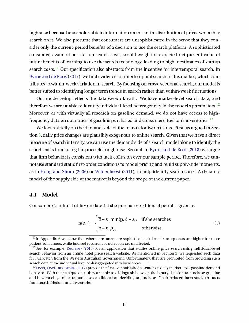
4.1 Model

Consumer i ’s indirect utility on date t if she purchases κi liters of petrol is given by

u(si t ) =u −κi min{pi t }− si t if she searches

u −κi p i t otherwise,(1)

11In Appendix A we show that when consumers are sophisticated, inferred startup costs are higher for morepatient consumers, while inferred recurrent search costs are unaffected.

12See, for example, Koulayev (2014) for an application that studies online price search using individual-levelsearch behavior from an online hotel price search website. As mentioned in Section 2, we requested such datafor Fuelwatch from the Western Australian Government. Unfortunately, they are prohibited from providing suchsearch data at the individual level or disaggregated into local areas.

13Levin, Lewis, and Wolak (2017) provide the first ever published research on daily market-level gasoline demandbehavior. With their unique data, they are able to distinguish between the binary decision to purchase gasolineand how much gasoline to purchase conditional on deciding to purchase. Their reduced-form study abstractsfrom search frictions and inventories.

11

where pi t is the vector of prices available to consumer i at date t , and si t is the current cost of

search for consumer i . As we discuss below, the set of stations available to consumer i is based

on geographic proximity to her home address, Li . This formulation assumes that if consumer i

on date t engages in price search on the clearinghouse, she becomes fully informed about the

price distribution and pays the minimum price in her local choice set, min{pi t }. If she does

not search, she pays the average price in her local choice set, p i t . Her gains from searching in

period t are

gi t = (p i t −min{pi t })×κi .

Consumer i ’s search costs in period t are given by

si t = fi × (1−wi t )+ ci ,

wi t = 1{consumer i has searched before date t },

where 1{·} is an indicator function, and fi and ci are consumer i ′s startup and recurrent search

costs, respectively. Recall that the Fuelwatch price clearinghouse allows consumers searching

after 2:30pm to discover prices for today and tomorrow. To account for this, consumer i con-

siders the gains from search in periods t and t + 1 when making her search decision on date

t :

yi t = 1{max{gi t , gi t+1} > si t }.

Define the type of consumer i as τi = ( fi ,ci ,Li ). We assume that fi , ci , and Li are inde-

pendent, and that the search costs fi and ci are drawn from gamma distributions (Hong and

Shum, 2006) with shape parameters µ f and µc and scale parameters σ f and σc , respectively.14

Consumer locations Li are drawn from the empirical distribution of population locations in the

market, as described below. We collect the search cost parameters into θ = [µ f ,σ f ,µc ,σ f ]′. Let

P be the distribution of consumer types. The predicted share of consumers engaging in online

price search on date t , qt (θ), is obtained by integrating over P :

qt (θ) =∫

yi t (τi ) dP (τi ;θ) =∫

yi t (τi ) dP f ( fi ;µ f ,σ f ) dPc (ci ;µc ,σc ) dPL(Li ). (2)

14We have estimated the model under alternative functional form assumptions, with no qualitative differencesin reported results. In particular, we have estimated the model under the assumption that fi and ci are drawn fromthe Log Normal distribution, both under the assumption that startup and recurrent search costs are independent,and allowing for correlation between them.

12

4.2 Estimation and identification

We estimate the model using a Simulated Minimum Distance estimator that compares the share

of searchers predicted by the model, qt (θ), to its empirical analogue, q̂t , computed as

q̂t = nt

Q,

where nt is the number of Fuelwatch website hits on date t , and the market size Q represents

the number of consumers considering a gasoline purchase each day.15

Computing q̂t requires us to make an assumption regarding the market size, Q. We com-

pute this as Q = (0.80×1,576,000)/7, which assumes that 80% of the population in Perth aged

between 15 and 79 years plans to fill up their car once every week, and does so uniformly by

day of the week. We calibrate the size of a gasoline purchase to κi = 50 liters for all consumers.

The most popular car in Australia is the Toyota Corolla, which has a 55 liter tank. According

to this calibration, each representative consumer fills up their Toyota Corolla when it is almost

empty.16

To construct the distribution of consumer locations PL , which determines the distribution

of gains from search, we partition the region of Greater Perth into local districts as classified

by the Australian Bureau of Statistics.17 For each district, we obtain driving age (18-79 years)

population and the location of the centroid of the district from the 2011 Census. By matching

this to the location of each station, we obtain the set of stations within a 5km radius.18 Average

and minimum prices for each district are defined with reference to this local set of stations. To

construct our simulated minimum distance estimator, we then assign each consumer randomly

to a district according to weights based on driving age population. By calculating local search

15By fixing the market size over time, we implicitly introduce an outside good into the model. Because someconsumers are aware of the cyclical nature of prices in this market, there is a cycle in sales volumes over the week.See, for example, Australian Competition and Consumer Commission (2014) on the existence of a demand cyclein the Perth market. Fixing the market size amounts to assuming that, each day, the same volume of consumersconsiders both whether to purchase gasoline and whether to use the search platform.

16Data sources for our calculations are as follows. From Australian Bureau of Statistics Table 3235.0, “Pop-ulation by Age and Sex, Regions of Australia”, there were 1,576,479 people aged between 15 and 79 years inthe greater Perth area on June 30, 2014. The Australian Competition and Consumer Commission (2007) re-port into the Australian petrol market commissioned a survey of 775 motorists in Australia, finding that 26%purchase more than once per week, 50% purchase once per week, 20% purchase every 2 weeks, and 4%purchase less than every 2 weeks. According to the Federal Chamber of Automotive Industries (FCAI), themost popular car in Australia in 2014 was the Toyota Corolla (see: https://www.drive.com.au/motor-news/the-10-most-popular-cars-of-2014-20150105-12ihkp). The fuel tank capacity for a Toyota Corolla is 55 liters (seehttp://www.toyota.com.au/corolla/specifications/ascent-sedan-manual).

17We use the finest classification available from the 2011 Census, known as Statistical Areas, Level 1. Of the 3789Statistical Areas in the Greater Perth region, the average district has 318.7 people (s.d. 128.3).

18Our main qualitative findings are unaffected by the choice of search radius. However, as we might expect, in-creasing the radius of search raises the value of information, and leads us to infer higher search costs. See AppendixB, where we also estimate the model using a 2km and a 10km search radius.

13

gains in this manner, we abstract from commuting patterns.19

Let et (θ) = qt (θ)− q̂t be the difference between the model’s prediction and the fraction of

searchers in the data at date t , and let e(θ) be the T ×1 vector of prediction errors, where T is

the number of dates in the sample. We estimate θ by minimizing the objective function20

θ̂ = argminθ

G(θ) = e(θ)′e(θ).

For a given value of θ, we compute G(θ) by forward simulating the search shares, qt (θ), for

each sample date t = 1, . . . ,T . To simulate search shares, we must keep track of each simulated

consumer’s history of search. Define the set of “active” consumers at the start of period t as

At = {i : wi ,t−1 = 1}.

For the forward simulation, we must initialise the set of active consumers at the start of the

sample period, A1. We use the maximum search intensity in the two weeks prior to the start of

the estimation sample to define A1. In particular, taking T0 to be the two week pre-sample, we

set the size of A1 equal to maxt∈T0 nt . We then assign active status randomly across consumers.

With this method, we estimate that 10% of consumers in the market have already sunk their

startup search costs at the start of the sample period.

Identification. The distribution of recurrent search costs is identified by periods in which the

benefits of search are unremarkable. Thus, variation in aggregate search activity associated with

variation in search gains, when such gains are moderate, identifies the parameters µc and σc .

By contrast, the startup search cost parameters µ f and σ f are identified by the responsiveness

of aggregate search to unprecedented gains from search arising from the price war. Finally, over

the sample period, aggregate search varies between 5% and 30% of consumers, which we show

in Figure 7 below. Therefore, estimation is well–suited for identifying the search cost distribu-

tion corresponding to this range of search intensities, but not necessarily the entire search cost

distribution.

14

Table 2: Search Model Estimation Results

With startup Without startupSearch Costs Search Costs

(1) (2)

Recurrent searchcost distribution

µc 0.202 0.611(0.016) (0.007)

σc 40.769 160.257(3.039) (5.475)

Startup searchcost distribution

µ f 5.070(0.086)

σ f 4.228(0.203)

Objective function, G(θ̂) 0.356 1.061

Notes: Robust standard errors are in parentheses. The number ofobservations is T = 731 dates. All calculations assume consumerspurchase 50 liters of gasoline.

4.3 Results

Estimation results are presented in Table 2. Column (1) contains estimates for the full model,

and column (2) contains estimates for a constrained model in which there are no startup search

costs. Panels (A) and (B) of Figure 6 present the cumulative density functions of the startup and

recurrent search cost distributions based on the point estimates of the model.

To illustrate the qualitative difference between the models, consider the 20th percentile con-

sumer in the search cost distributions. For the model with startup search costs, the 20th per-

centile startup costs are $13.30/day. Conditional on having sunk this startup cost, the 20th

percentile recurrent search cost is $0.01/day.21 In the model without startup search costs, esti-

mated recurrent search costs are an order of magnitude greater. In this model, the 20thpercentile

consumer has recurrent search cost of $9.94. This conforms with intuition, as these recurrent

search cost estimates are driven by both startup search costs and recurrent search costs.

19See Pennerstorfer et al. (2017) for an analysis of commuting routes and search incentives.20We use the following optimization procedure. We calculate the objective function G(θ) for a grid of parameters.

We calculate the minimum of G(θ) across the grid, and select all parameter vectors with a value of G(θ) that iswithin 10% of the minimum. We then perform a Nelder-Mead optimization for each of these parameter vectors.For our final estimates, we take 100,000 draws from P to evaluate the integral in equation (2).

21Note that, because startup and nonsequential search costs are independently drawn, one cannot simply addthe 20th percentile of each distribution to obtain the 20th percentile aggregate search cost.

15

Turning to model fit, from Table 2 we find the econometric objective function for the full

model of G(θ̂) = 0.356 is substantially lower than the model without startup search costs, where

G(θ̂) = 1.061. Figure 7 further describes the implications for model fit from accounting for

startup search costs. Panel A shows that, despite being simple, our model with startup costs is

able to recreate the amplitude and frequency of search cycles, with the amplitude being some-

what underestimated. Importantly, the full model precisely fits the sharp and permanent shift

in search intensity after the temporary shock to search incentives caused by the price war.

Panel B of Figure 7 yields a stark contrast for the restricted model without startup costs. In

this model, the distribution of recurrent search costs is identified by variation in search activity

with search benefits, both when those benefits are unprecedented and when they are moderate.

While the model is able to capture the amplitude and frequency of search cycles, the model is

unable to produce a permanent shift in search behavior after the shock. As the gains from

search return to baseline following the shock, in the absence of startup costs, the standard non-

sequential search model predicts search intensity will also return to baseline.

Finally, panel C shows the predicted evolution of consumer experience with search. In grey

(left scale), we depict the population-weighted average gains from search, and in the foreground

(right scale), we show the predicted fraction of active consumers. The fraction of consumers

who have incurred startup search costs is approximately a step function over time. When the

gains from search are abnormally high in the middle of the sample, the predicted fraction of

consumers with search experience grows rapidly from 12% to 18%.

Panel C further helps to explain the differential performance of the two models. In the full

model, following the price war, a greater fraction of consumers have experience with search.

This changes the aggregate relationship between search activity and search benefits, and ex-

plains why search remains elevated after search benefits decline. By contrast, the restricted

model does not allow for a dynamic relationship between search activity and search benefits,

and therefore predicts that search activity must rise and fall with current search gains.

5 Summary and discussion

In studying search frictions, economists have, to date, assumed that search costs are indepen-

dent of search history. Exploiting a natural experiment in retail gasoline, together with unique

data on retail prices and search behavior, we have provided evidence on a new form of search

costs that we call startup search costs. The novel evidence of history dependence in search be-

havior that we find suggests that the first search cost sunk by a consumer is drastically different

from subsequent search costs. Search experience matters.

The results from our simple empirical search model highlight the implications of startup

16

Figure 6: Search Cost Distributions

Panel A: Startup Search Costs

0 10 20 30 40 50 60 70 80

Startup search costs ($AU)

00

.10

.20

.30

.40

.50

.60

.70

.80

.91

Cu

mu

lative

de

nsity

Panel B: Recurrent Search Costs

0 10 20 30 40 50 60 70 80

Recurrent search costs ($AU)

00

.10

.20

.30

.40

.50

.60

.70

.80

.91

Cu

mu

lative

de

nsity

Model with startup costs

Model without startup costs

search costs for the measurement of search frictions. Model misspecification that ignores startup

search costs yields overestimated recurrent search costs. Moreover, we have shown how a stan-

dard non-sequential search model is unable to account for a permanent rise in market-level

search from a temporary exogenous shock to search incentives.

Because we work with market-level and not individual-level search data, we are unable to

identify deeper microfoundations for startup search costs.We can think of at least four possible

mechanisms to explore in future research. First, startup search costs could be driven by tech-

nology adoption costs (Foster and Rosenzweig, 2010) with online price clearinghouses. Second,

startup search costs could reflect consumers holding biased beliefs about the value of search

(Koulayev and Alexandrov, 2017), and updating these beliefs after trialing the clearinghouse

during the price war. Third, consumers could rapidly form habits after trialing the clearing-

house (Becker and Murphy, 1988) with minimal rates of habit decay. Finally, the inertia in non-

adoption of the clearinghouse for 15 years before the war, followed by a permanent shift in

usage after, could reflect procrastination or time-inconsistency (O’Donoghue and Rabin, 1999)

in trialing and learning to use the clearinghouse.

Understanding the role of startup search costs and their underlying mechanisms is impor-

tant for policy. We believe that the evidence presented here points to a new and important

policy challenge with online search platforms aimed at promoting price transparency and mar-

ket efficiency: policymakers need to get consumers “over the hump” in starting to use such

platforms. We have found that this hump prevented consumers from engaging with a well-

established price clearinghouse for 15 years. It took a three-week, temporary price shock to

substantially increase online price search by 70% more than a decade and a half after the clear-

inghouse was established. The lesson for policy is that large, temporary shocks to search in-

17

Figure 7: Search Model Predictions

Panel A: Non-Sequential Search Modelwith Startup Search Costs

Jul 2014 Jan 2015 Jul 2015 Jan 2016 Jul 2016

Date

00

.05

0.1

0.1

50

.20

.25

0.3

Sh

are

of

se

arc

he

rs

Data

Model prediction

Panel B: Non-Sequential Searchwithout Startup Search Costs


Date

00

.05

0.1

0.1

50

.20

.25

0.3

Sh

are

of

se

arc

he

rs

Data

Model prediction

Panel C: Gains from Search


Date

1

2

3

4

5

6

7

8

9

10

Gain

s fro

m s

earc

h

0.1

0.1

10.1

20.1

30.1

40.1

50.1

60.1

70.1

80.1

9

Pre

dic

ted s

hare

of active c

onsum

ers

Search gains

Active consumers

centives can help consumers overcome startup search costs and lead to long-run adoption of

search platforms. Policy interventions that encourage customers to experiment with such plat-

forms are a potential remedy for overcoming startup search costs.

On the supply-side, our study raises a separate question for future research: what is the

impact of startup search costs for firms’ pricing decision? In the retail gasoline market that

we study, we obtain an interesting implication for firms’ pricing decisions. As we have men-

tioned, in Byrne and de Roos (2018) we document evidence consistent with tacit collusion in

this market. In this context, by encouraging consumers to engage with search, the temporary

price war may have led to an increase in demand elasticity, and therefore collusive outcomes

may have become more difficult to sustain following the war. This suggests a new trade-off –

price variation could lead to a sustained increase in demand elasticity – facing cartel members

18

contemplating either an adjustment of pricing policies or defection from a cartel.

19

Appendix

A Consumers with a dynamic perspective

In the model of Section 4, we presumed consumers take a static perspective when deciding

whether to incur startup search costs. In this section, we illustrate the implications of relaxing

this assumption. Consider the perspective of consumer i who evaluates the impact of today’s

search decision on the search environment that she will face in the future. To fix ideas, we begin

by laying out the Bellman equation faced by consumer i at time t when she adopts this dynamic

perspective.

Given current search state wi t , her type τi , and price vector pi t , her current valuation is

given by

V (wi t ) = maxχi t∈{0,1}

χi t(u −κi min{pi t }− si t

)+ (1−χi t )(u −κi p i t

)+δEt V (wi t+1),

wi t+1 = wi t + (1−wi t )χi t ,

where χi t = 1 indicates a decision to search today and χi t = 0 indicates no search; and Et in-

dicates period-t expectations over future price distributions.22 The parameter δ describes the

rate at which consumers discount the next fuel purchase, and could reflect impatience, and

concerns about the decay or obsolecence of current knowledge of the search process.

Expectations of future prices play an important role through their influence on the contin-

uation value of the consumer’s dynamic problem. For illustration, we consider a simple expec-

tations process. We say that consumer i adopts stationary expectations if she anticipates the

current price distribution to be observed in subsequent periods: pt+k = pt , for k > 0. This leads

to the following proposition.

Proposition 1. Suppose consumer j adopts a static perspective with search costs c j and f j , and

consumer i adopts a dynamic perspective with stationary expectations and search costs ci and fi .

Then consumers i and j are observationally equivalent if ci = c j and fi = f j /(1−δ).

Proof. First, consider consumer j . Based on her static perspective, she searches iff g j t > s j t . If

w j t = 1, she searches iff g j t > c j ; if w j t = 0, she searches iff g j t > c j + f j .

Next, consider consumer i and suppose wi t = 1. In this case, she has already sunk her

startup search costs and, as a result, her current search decision has no dynamic consequences.

22For simplicity, we ignore the intertemporal searh opportunities presented by the Fuelwatch program in thisformulation, and consider search gains in period t based solely on the period t price distribution.

20

Thus, she chooses to search iff gi t > ci . Because wi t = 1 is an absorbing state, we can solve for

the value V (1) = u(ci )/(1−δ), where u(.) is defined in equation (1).

Suppose instead wi t = 0 and observe that consumer i has value

V (0) = maxχi t∈{0,1}

χi t(u −κi min{pi t }− ci − fi

)+ (1−χi t )(u −κi p i t

)+δ

(χi t V (1)+ (1−χi t )V (0)

).

Consumer i searches in period t iff

u −κi min{pi t }− ci − fi +δu(ci )

1−δ> u −κi p i t +δV (0).

Observing that consumer i makes the same decision whenever wi t = 0, we can deduce that she

searches iff

(1−δ)(u −κi min{pi t }− ci − fi

)+δu(ci ) > u −κi p i t . (3)

Next, we show that, when wi t = 0, consumer i searches iff gi t > ci + (1−δ) fi . We break this

into two steps. First, observe that if gi t > ci , then a consumer who had already sunk her startup

search costs would choose to search. This means that u(ci ) = u −κi min{pi t }− ci . Substituting

into (3) leads to the conclusion that i searches iff gi t > ci + (1−δ) fi . Next, suppose that gi t ≤ ci .

In this case, u(ci ) = u −κi p t . Suppose further that χi t = 1. Substituting into (3) leads to the

condition gi t > ci + fi , a contradiction. Therefore χi t = 0 whenever gi t ≤ ci . Combining the two

cases, we have our desired result that consumer i searches iff gi t > ci + (1−δ) fi .

Finally, comparing consumers i and j leads to the conclusion that their choices are identical

if ci = c j and (1−δ) fi = f j , as required.

Proposition 1 gives a feeling for the impact of the consumer’s perspective on inferences

about search costs under the assumption of stationary expectations. The perspective adopted

by consumer i has no impact on the inferences we make about her recurrent search costs.

However, particularly for patient consumers, inferred startup search costs will be substantially

higher if we presume consumers adopt a dynamic perspective.

The logic of the proof of Proposition 1 provides an indication of the impact of the assump-

tion of stationary expectations. Suppose that in period t , consumer i decides to first engage

in search. Under the stationarity assumption, she anticipates that she would also have chosen

to initiate search in period t +1 had she not chosen to search in period t . Thus, she derives a

benefit of fi in every subsequent period. Similarly, if instead she anticipates that price variation

and the gains to search will increase over time, then she will also anticipate engaging in search

21

in each period, and the value to her of initiating search will be the same. Alternatively, if she

expects the gains to search to fall, she may anticipate that there are future periods in which she

would not be willing to initiate search. In this case, by assuming stationarity, startup search

costs will be overestimated.

B Specification of search gains: robustness

Recall that the gains to search for consumer i at time t are defined by

gi t = (p i t −min{pit})×κi .

In the body of the paper, we presumed that average and minimum prices for consumer i were

taken with respect stations within a 5km radius of the centroid of her local district. In this

section, we also consider search radii of 2km and 10km.

As the search radius varies between 2km and 10km, there is a noticeable impact on the

consumer’s choice set. With a search radius of 2km, 5km, and 10km, there are on average 1.96

stations (s.d. 1.57), 10.29 stations (s.d. 6.32), and 34.26 stations (s.d. 18.86) within the choice

radius for each district. For estimation purposes, we eliminate all districts with less than two

stations inside the search radius.

For comparability, we retain the same format for the presentation of results. Table 3 con-

tains estimation results. Columns (1) and (2) ((3) and (4)) contain estimates based on a 2km

(10km) search radius. For each specification of the search radius, the left and right columns

contain, respectively, esimates based on the full model and a constrained model that does not

include startup search costs. Figures 8 and 9 depict, for the 2km search radius specification, the

cumulative distribution of estimated startup and recurrent search costs, and predictions for

the model, respectively. Figures 10 and 11 contain analogous information for the 10km search

radius specification.

The main qualitative features we highlighted earlier carry over to alternative specifications

of the search radius. In particular, the model with startup costs leads to qualitatively different

inferences over recurrent search costs, the fit of the model is much improved by incorporating

startup search costs, and only the model with startup search costs is able to explain the perma-

nent increase in search activity following the temporary shock to search gains.

Adjusting the search radius does lead to some variation in results. When the search radius

is reduced, measured search gains tend to be lower. This can be seen by comparing Panel C

of Figures 7, 9, and 11. As a result, to rationalize observed search activity, estimated startup

and recurrent search costs are lower when the search radius is reduced. This is best seen by

22

Table 3: Estimation Results with Alternative Search Radii

2km Search Radius 10km Search RadiusWith Without With Without

Startup Costs Startup Costs Startup Costs Startup Costs(1) (2) (3) (4)

Recurrent searchcost distribution

µc 0.205 0.455 0.215 0.421(0.017) (0.005) (0.017) (0.003)

σc 16.907 176.596 36.781 1322.721(2.341) (6.759) (3.829) (17.370)

Startup searchcost distribution

µ f 1.945 6.201(0.081) (0.144)

σ f 12.110 3.811(0.613) (0.135)

Objective function, G(θ̂) 0.374 0.816 0.375 0.934

Notes: Robust standard errors are in parentheses (). The number of observations is T = 731 dates. Allcalculations assume consumers purchase 50 liters of gasoline.

comparing Figures 6, 8, and 10. Consider first the model with startup search costs. Estimated

20thpercentile startup costs are $9.54, $13.30, and $15.51 when the search radius is 2km, 5km,

and 10km, respectively. At the left tail of the distribution, estimated recurrent search costs are

negligible in each specification of the search radius. The change to our search gain specification

makes a bigger difference to estimates for the model without startup search costs. The 20th

percentile consumer now has estimated recurrent search costs of $3.98, $9.94, and $22.06 when

the search radius is 2km, 5km, and 10km, respectively.

Comparing Figure 9 and 11 reveals some subtle differences in model predictions. When

search gains are defined more locally, this accentuates the volatility in search gains, and there

is an associated increase in the high-frequency volatility in predicted search, both for the full

model (Panel A) and the restricted model without startup search costs (Panel B). Finally, Panel

C also suggests that, when search gains are defined more locally, to rationalize the volume of

search activity, a greater proportion of consumers are predicted to incur their startup search

costs.

23

Figure 8: Search Cost Distributions, 2km Search Radius


0 10 20 30 40 50 60 70 80


00

.10

.20

.30

.40

.50

.60

.70

.80

.91

Cu

mu

lative

de

nsity

Panel B: Recurrent Search Costs

0 10 20 30 40 50 60 70 80


00

.10

.20

.30

.40

.50

.60

.70

.80

.91

Cu

mu

lative

de

nsity



24

Figure 9: Search Model Predictions, 2km Search Radius



Date

00

.05

0.1

0.1

50

.20

.25

0.3

Sh

are

of

se

arc

he

rs

Data

Model prediction



Date

00

.05

0.1

0.1

50

.20

.25

0.3

Sh

are

of

se

arc

he

rs

Data

Model prediction



Date

0

1

2

3

4

5

6

Ga

ins f

rom

se

arc

h

0.1

0.1

10

.12

0.1

30

.14

0.1

50

.16

0.1

70

.18

0.1

90

.2

Pre

dic

ted

sh

are

of

active

co

nsu

me

rs

Search gains

Active consumers

25

Figure 10: Search Cost Distributions, 10km Search Radius


0 10 20 30 40 50 60 70 80


00

.10

.20

.30

.40

.50

.60

.70

.80

.91

Cu

mu

lative

de

nsity

Panel B: Recurrent Search Cost

0 10 20 30 40 50 60 70 80


00

.10

.20

.30

.40

.50

.60

.70

.80

.91

Cu

mu

lative

de

nsity



26

Figure 11: Search Model Predictions, 10km Search Radius



Date

00

.05

0.1

0.1

50

.20

.25

0.3

Sh

are

of

se

arc

he

rs

Data

Model prediction



Date

00

.05

0.1

0.1

50

.20

.25

0.3

Sh

are

of

se

arc

he

rs

Data

Model prediction



Date

0

2

4

6

8

10

12

14

Gain

s fro

m s

earc

h

0.1

0.1

10.1

20.1

30.1

40.1

50.1

60.1

70.1

8

Pre

dic

ted s

hare

of active c

onsum

ers

Search gains

Active consumers

27

References

Australian Competition and Consumer Commission. Petrol prices and Australian consumers.

Report of the ACCC Inquiry into the Price of Unleaded Petrol, 2007.

Australian Competition and Consumer Commission. Petrol prices and Australian consumers.

Report of the ACCC Inquiry into the Price of Unleaded Petrol, 2014.

Australian Competition and Consumer Commission. Report on the australian petroleum mar-

ket, september quarter 2017, 2017.

Michael R. Baye, John Morgan, and Patrick Scholten. Information, search, and price dispersion.

2006. Chapter 6 in Handbook in Economics and Information Systems Vol. 1 (T. Hendershott,

Ed.), Amsterdam: Elsevier.

Gary S. Becker and Kevin M. Murphy. A theory of rational addiction. Journal of Political Econ-

omy, 96:675–700, 1988.

Tom Blake, Dominic Coey, Kane Sweeney, and Steve Tadelis. Price salience and product choice.

NBER Working paper 25186, 2018.

Nicholas Buchholz. Spatial equilibrium, search frictions and dynamic efficiency in the taxi in-

dustry. mimeo, Princeton University, 2018.

David P. Byrne and Nicolas de Roos. Consumer search in retail gasoline markets. Journal of

Industrial Economics, 65:183–193, 2017.

David P. Byrne and Nicolas de Roos. Learning to coordinate: A study in retail gasoline. American

Economic Review, 2018. forthcoming.

Vincent P. Crawford, Miguel A. Costa-Comes, and Nagore Iriberri. Structural models of nonequi-

lbrium strategic thinking: Theory, evidence, and applications. Journal of Economic Literature,

51:5–62, 2013.

Babur de Los Santos, Ali Hortascu, and Matthijs R. Wildenbeest. Testing models of consumers

search using data on web browsing and purchasing behavior. American Economic Review,

102:2955–2980, 2012.

Andrew Eckert. Empirical studies of gasoline retailing: A guide to the literature. Journal of

Economic Surveys, 27:140–166, 2013.

28

Sara Fisher Ellison. Price search and obfuscation: an overview of the theory and empirics.

Handbook of the Economics of Retail and Distribution, 2016. Emek Basker (eds), Elgar.

Andrew D. Foster and Mark R. Rosenzweig. Microeconomics of technology adoption. Annual

Review of Economics, 2:395–424, 2010.

Han Hong and Matthew Shum. Using price distributions to estimate search costs. RAND Jour-

nal of Economics, 37, 2006.

Sergei Koulayev. Search for differentiated products: Identification and estimation. Rand Journal

of Economics, 45:553–575, 2014.

Sergei Koulayev and Alexei Alexandrov. No shopping in the u.s. mortgage market: Direct and

strategic effects of providing information. CFPB Working Paper 2017-01, 2017.

Laurence Levin, Matthew S. Lewis, and Frank A. Wolak. High frequency evidence on the de-

mand for gasoline. American Economic Journal: Economic Policy, 9, 2017.

Ted O’Donoghue and Matthew Rabin. Doing it now or later. American Economic Review, 89:

104–124, 1999.

Dieter Pennerstorfer, Philipp Schmidt-Dengler, Nicolas Schutz, Christoph Weiss, and Biliana

Yontcheva. Information and price dispersion: Theory and evidence. CEPR Discussion Paper

10771, 2017.

Stephan Seiler and Fabio Pinna. Estimating search benefits from path-tracking data: Measure-

ments and determinants. Marketing Science, 36:565–589, 2017.

Meredith Startz. The value of face-to-face: Search and contracting problems in nigerian trade.

mimeo, Stanford University, 2018.

George J. Stigler. The economics of information. Journal of Political Economy, 69:213–225, 1961.

Matthijs R. Wildenbeest. An empirical model of search with vertically differentiated products.

Rand Journal of Economics, 42:729–757, 2011.

29

Startup Search Costs

Documents

Transcript of Startup Search Costs