Designation: E1820 − 13´1

Standard Test Method forMeasurement of Fracture Toughness1

This standard is issued under the fixed designation E1820; the number immediately following the designation indicates the year oforiginal adoption or, in the case of revision, the year of last revision. A number in parentheses indicates the year of last reapproval. Asuperscript epsilon (´) indicates an editorial change since the last revision or reapproval.

ε1 NOTE—Sections A6.2.2 and A6.3.2 were editorially revised in May 2015.

1. Scope

1.1 This test method covers procedures and guidelines forthe determination of fracture toughness of metallic materialsusing the following parameters: K, J, and CTOD (δ). Tough-ness can be measured in the R-curve format or as a point value.The fracture toughness determined in accordance with this testmethod is for the opening mode (Mode I) of loading.

NOTE 1—Until this version, KIc could be evaluated using this testmethod as well as by using Test Method E399. To avoid duplication, theevaluation of KIc has been removed from this test method and the user isreferred to Test Method E399.

1.2 The recommended specimens are single-edge bend,[SE(B)], compact, [C(T)], and disk-shaped compact, [DC(T)].All specimens contain notches that are sharpened with fatiguecracks.

1.2.1 Specimen dimensional (size) requirements vary ac-cording to the fracture toughness analysis applied. The guide-lines are established through consideration of materialtoughness, material flow strength, and the individual qualifi-cation requirements of the toughness value per values sought.

1.3 The values stated in SI units are to be regarded as thestandard. The values given in parentheses are for informationonly.

1.4 This standard does not purport to address all of thesafety concerns, if any, associated with its use. It is theresponsibility of the user of this standard to establish appro-priate safety and health practices and determine the applica-bility of regulatory limitations prior to use.

NOTE 2—Other standard methods for the determination of fracturetoughness using the parameters K, J, and CTOD are contained in TestMethods E399, E1290, and E1921. This test method was developed toprovide a common method for determining all applicable toughnessparameters from a single test.

2. Referenced Documents

2.1 ASTM Standards:2

E4 Practices for Force Verification of Testing MachinesE8/E8M Test Methods for Tension Testing of Metallic Ma-

terialsE21 Test Methods for Elevated Temperature Tension Tests of

Metallic MaterialsE23 Test Methods for Notched Bar Impact Testing of Me-

tallic MaterialsE399 Test Method for Linear-Elastic Plane-Strain Fracture

Toughness KIc of Metallic MaterialsE1290 Test Method for Crack-Tip Opening Displacement

(CTOD) Fracture Toughness Measurement (Withdrawn2013)3

E1823 Terminology Relating to Fatigue and Fracture TestingE1921 Test Method for Determination of Reference

Temperature, To, for Ferritic Steels in the TransitionRange

E1942 Guide for Evaluating Data Acquisition Systems Usedin Cyclic Fatigue and Fracture Mechanics Testing

E2298 Test Method for Instrumented Impact Testing ofMetallic Materials

3. Terminology

3.1 Terminology E1823 is applicable to this test method.Only items that are exclusive to Test Method E1820, or thathave specific discussion items associated, are listed in thissection.

3.2 Definitions of Terms Specific to This Standard:3.2.1 compliance [LF−1], n—the ratio of displacement in-

crement to force increment.

3.2.2 crack opening displacement (COD) [L], n—force-induced separation vector between two points at a specific gagelength. The direction of the vector is normal to the crack plane.

1 This test method is under the jurisdiction of ASTM Committee E08 on Fatigueand Fracture and is the direct responsibility of Subcommittee E08.07 on FractureMechanics.

Current edition approved Nov. 15, 2013. Published January 2014. Originallyapproved in 1996. Last previous edition approved in 2011 as E1820 – 11 ε2. DOI:10.1520/E1820-13E01.

2 For referenced ASTM standards, visit the ASTM website, www.astm.org, orcontact ASTM Customer Service at service@astm.org. For Annual Book of ASTMStandards volume information, refer to the standard’s Document Summary page onthe ASTM website.

3 The last approved version of this historical standard is referenced onwww.astm.org.

Copyright © ASTM International, 100 Barr Harbor Drive, PO Box C700, West Conshohocken, PA 19428-2959. United States

1

3.2.2.1 Discussion—In this practice, displacement, v, is thetotal displacement measured by clip gages or other devicesspanning the crack faces.

3.2.3 crack extension, ∆a [L], n—an increase in crack size.

3.2.4 crack-extension force, G [FL−1 or FLL−2], n—theelastic energy per unit of new separation area that is madeavailable at the front of an ideal crack in an elastic solid duringa virtual increment of forward crack extension.

3.2.5 crack size, a [L], n—a lineal measure of a principalplanar dimension of a crack. This measure is commonly usedin the calculation of quantities descriptive of the stress anddisplacement fields, and is often also termed crack length ordepth.

3.2.5.1 Discussion—In practice, the value of a is obtainedfrom procedures for measurement of physical crack size, ap,original crack size, ao, and effective crack size, ae , asappropriate to the situation being considered.

3.2.6 crack-tip opening displacement (CTOD), δ [L], n—thecrack displacement resulting from the total deformation (elasticplus plastic) at variously defined locations near the originalcrack tip.

3.2.6.1 Discussion—In this test method, CTOD is the dis-placement of the crack surfaces normal to the original (un-loaded) crack plane at the tip of the fatigue precrack, ao . In thistest method, CTOD is calculated at the original crack size, ao,from measurements made from the force versus displacementrecord.

3.2.6.2 Discussion—In CTOD testing, δIc [L] is a value ofCTOD near the onset of slow stable crack extension, heredefined as occurring at ∆ap = 0.2 mm (0.008 in.) + 0.7δIc.

3.2.6.3 Discussion—In CTOD testing, δc [L] is the value ofCTOD at the onset of unstable crack extension (see 3.2.39) orpop-in (see 3.2.25) when ∆ap <0.2 mm (0.008 in.) + 0.7δc. δc

corresponds to the force Pc and clip-gage displacement vc (seeFig. 1). It may be size-dependent and a function of testspecimen geometry.

3.2.6.4 Discussion—In CTOD testing, δu [L] is the value ofCTOD at the onset of unstable crack extension (see 3.2.39) orpop-in (see 3.2.25) when the event is preceded by ∆ap >0.2 mm(0.008 in.) + 0.7δu. The δu corresponds to the force Pu and theclip gage displacement vu (see Fig. 1). It may be size-dependent and a function of test specimen geometry. It can beuseful to define limits on ductile fracture behavior.

3.2.6.5 Discussion—In CTOD testing, δc* [L] characterizes

the CTOD fracture toughness of materials at fracture instabilityprior to the onset of significant stable tearing crack extension.The value of δc

* determined by this test method represents ameasure of fracture toughness at instability without significantstable crack extension that is independent of in-plane dimen-sions. However, there may be a dependence of toughness onthickness (length of crack front).

3.2.7 dial energy, KV [FL]—absorbed energy as indicatedby the impact machine encoder or dial indicator, as applicable.

3.2.8 dynamic stress intensity factor, KJd—The dynamicequivalent of the stress intensity factor KJ, calculated from Jusing the equation specified in this test method.

3.2.9 dynamic ultimate tensile strength, σTSd [FL-2]—dynamic equivalent of the ultimate tensile strength, measuredat the equivalent strain rate of the fracture toughness test.

3.2.10 dynamic yield strength, σYSd [FL-2]—dynamicequivalent of the yield strength, measured at the equivalentstrain rate of the fracture toughness test.

3.2.11 effective thickness, Be [L] , n—for side-groovedspecimens Be = B − (B − BN)2/B. This is used for the elasticunloading compliance measurement of crack size.

3.2.12 effective yield strength, σY [FL−2], n—an assumedvalue of uniaxial yield strength that represents the influence ofplastic yielding upon fracture test parameters.

3.2.12.1 Discussion—It is calculated as the average of the0.2 % offset yield strength σYS, and the ultimate tensilestrength, σTS as follows:

NOTE 1—Construction lines drawn parallel to the elastic loading slope to give vp, the plastic component of total displacement, vg.NOTE 2—In curves b and d, the behavior after pop-in is a function of machine/specimen compliance, instrument response, etc.

FIG. 1 Types of Force versus Clip Gage Displacement Records

E1820 − 13´1

2

σY 5σYS1σTS

2(1)

3.2.12.2 Discussion—In estimating σY, influences of testingconditions, such as loading rate and temperature, should beconsidered.

3.2.12.3 Discussion—The dynamic effective yield strength,σYd, is the dynamic equivalent of the effective yield strength,and is calculated as the average of the dynamic yield strengthand dynamic ultimate tensile strength.

3.2.13 general yield force, Pgy [F] —in an instrumentedimpact test, applied force corresponding to general yielding ofthe specimen ligament. It corresponds to Fgy, as used in TestMethod E2298.

3.2.14 J-integral, J [FL−1], n—a mathematical expression, aline or surface integral that encloses the crack front from onecrack surface to the other, used to characterize the localstress-strain field around the crack front.

3.2.14.1 Discussion—The J-integral expression for a two-dimensional crack, in the x-z plane with the crack front parallelto the z-axis, is the line integral as follows:

J 5 *ΓS Wdy 2 T ·

] u] x

dsD (2)

where:W = loading work per unit volume or, for elastic bodies,

strain energy density,Γ = path of the integral, that encloses (that is, contains)

the crack tip,ds = increment of the contour path,T = outward traction vector on ds,u = displacement vector at ds,x, y, z = rectangular coordinates, and

T ·] u]x

ds= rate of work input from the stress field into the area

enclosed by Γ.

3.2.14.2 Discussion—The value of J obtained from thisequation is taken to be path-independent in test specimenscommonly used, but in service components (and perhaps in testspecimens) caution is needed to adequately consider loadinginterior to Γ such as from rapid motion of the crack or theservice component, and from residual or thermal stress.

3.2.14.3 Discussion—In elastic (linear or nonlinear) solids,the J-integral equals the crack-extension force, G. (See crackextension force.)

3.2.14.4 Discussion—In elastic (linear and nonlinear) solidsfor which the mathematical expression is path independent, theJ-integral is equal to the value obtained from two identicalbodies with infinitesimally differing crack areas each subject tostress. The parameter J is the difference in work per unitdifference in crack area at a fixed value of displacement or,where appropriate, at a fixed value of force (1)4.

3.2.14.5 Discussion—The dynamic equivalent of Jc isJcd,X, with X = order of magnitude of J-integral rate.

3.2.15 Jc [FL−1] —The property Jc determined by this testmethod characterizes the fracture toughness of materials at

fracture instability prior to the onset of significant stabletearing crack extension. The value of Jc determined by this testmethod represents a measure of fracture toughness at instabil-ity without significant stable crack extension that is indepen-dent of in-plane dimensions; however, there may be a depen-dence of toughness on thickness (length of crack front).

3.2.16 Ju [FL−1]—The quantity Ju determined by this testmethod measures fracture instability after the onset of signifi-cant stable tearing crack extension. It may be size-dependentand a function of test specimen geometry. It can be useful todefine limits on ductile fracture behavior.

3.2.16.1 Discussion—The dynamic equivalent of Ju is Jud,X,with X = order of magnitude of J-integral rate.

3.2.17 J-integral rate, J @FL21T21#—derivative of J withrespect to time.

3.2.18 machine capacity, MC [FL]—maximum availableenergy of the impact testing machine.

3.2.19 maximum force, Pmax [F]—in an instrumented im-pact test, maximum value of applied force. It corresponds toFm, as used in Test Method E2298.

3.2.20 net thickness, BN [L], n—distance between the rootsof the side grooves in side-grooved specimens.

3.2.21 original crack size, ao [L] , n—the physical crack sizeat the start of testing.

3.2.21.1 Discussion—In this test method, aoq is used todenote original crack size estimated from compliance.

3.2.22 original remaining ligament, bo [L], n—distancefrom the original crack front to the back edge of the specimen,that is (bo = W − ao ).

3.2.23 physical crack size, ap [L] , n—the distance from areference plane to the observed crack front. This distance mayrepresent an average of several measurements along the crackfront. The reference plane depends on the specimen form, andit is normally taken to be either the boundary, or a planecontaining either the load-line or the centerline of a specimenor plate. The reference plane is defined prior to specimendeformation.

3.2.24 plane-strain fracture toughness, JIc [FL−1], KJIc

[FL−3/2] , n—the crack-extension resistance under conditionsof crack-tip plane-strain.

3.2.24.1 Discussion—For example, in Mode I for slow ratesof loading and substantial plastic deformation, plane-strainfracture toughness is the value of the J-integral designated JIc

[FL−1 ] as measured using the operational procedure (andsatisfying all of the qualification requirements) specified in thistest method, that provides for the measurement of crack-extension resistance near the onset of stable crack extension.

3.2.24.2 Discussion—For example, in Mode I for slow ratesof loading, plane-strain fracture toughness is the value of thestress intensity designated KJIc calculated from JIc using theequation (and satisfying all of the qualification requirements)specified in this test method, that provides for the measurementof crack-extension resistance near the onset of stable crackextension under dominant elastic conditions (2).

3.2.24.3 Discussion—The dynamic equivalent of JIc is JIcd,X

, with X = order of magnitude of J-integral rate.4 The boldface numbers in parentheses refer to the list of references at the end of

this standard.

E1820 − 13´1

3

3.2.25 pop-in, n—a discontinuity in the force versus clipgage displacement record. The record of a pop-in shows asudden increase in displacement and, generally a decrease inforce. Subsequently, the displacement and force increase toabove their respective values at pop-in.

3.2.26 R-curve or J-R curve, n—a plot of crack extensionresistance as a function of stable crack extension, ∆ap or ∆ae.

3.2.26.1 Discussion—In this test method, the J-R curve is aplot of the far-field J-integral versus the physical crackextension, ∆ap. It is recognized that the far-field value of J maynot represent the stress-strain field local to a growing crack.

3.2.27 remaining ligament, b [L], n—distance from thephysical crack front to the back edge of the specimen, that is(b = W − ap).

3.2.28 specimen center of pin hole distance, H* [L], n—thedistance between the center of the pin holes on a pin-loadedspecimen.

3.2.29 specimen gage length, d [L], n—the distance be-tween the points of displacement measure (for example, clipgage, gage length).

3.2.30 specimen span, S [L], n—the distance between speci-men supports.

3.2.31 specimen thickness, B [L], n—the side-to-side di-mension of the specimen being tested.

3.2.32 specimen width, W [L], n—a physical dimension ona test specimen measured from a reference position such as thefront edge in a bend specimen or the load-line in the compactspecimen to the back edge of the specimen.

3.2.33 stable crack extension [L], n—a displacement-controlled crack extension beyond the stretch-zone width (see3.2.37). The extension stops when the applied displacement isheld constant.

3.2.34 strain rate, ε—derivative of strain ε with respect totime.

3.2.35 stress-intensity factor, K, K1, K2, K3, KI, KII, KIII

[FL−3/2], n—the magnitude of the ideal-crack-tip stress field(stress-field singularity) for a particular mode in ahomogeneous, linear-elastic body.

3.2.35.1 Discussion—Values of K for the Modes 1, 2, and 3are given by the following equations:

K1 5 r→0lim @σyy~2πr!1/2# (3)

K2 5 r→0lim @τ xy~2πr!1/2# (4)

K3 5 r→0lim @τyz~2πr!1/2# (5)

where r = distance directly forward from the crack tipto a location where the significant stress is calculated.3.2.35.2 Discussion—In this test method, Mode 1 or Mode

I is assumed. See Terminology E1823 for definition of mode.

3.2.36 stress-intensity factor rate, K [FL-3/2T-1]—derivative of K with respect to time.

3.2.37 stretch-zone width, SZW [L], n—the length of crackextension that occurs during crack-tip blunting, for example,prior to the onset of unstable brittle crack extension, pop-in, orslow stable crack extension. The SZW is in the same plane as

the original (unloaded) fatigue precrack and refers to anextension beyond the original crack size.

3.2.38 time to fracture, tf [T]—time corresponding to speci-men fracture.

3.2.39 unstable crack extension [L], n—an abrupt crackextension that occurs with or without prior stable crackextension in a standard test specimen under crosshead or clipgage displacement control.

3.3 Symbols:3.3.1 ti [T]—time corresponding to the onset of crack

propagation.

3.3.2 v0 [LT-1]—in an instrumented impact test, strikervelocity at impact.

3.3.3 Wm [FL]—in an instrumented impact test, absorbedenergy at maximum force.

3.3.4 Wt [FL]—in an instrumented impact test, total ab-sorbed energy calculated from the complete force/displacementtest record.

3.3.5 W0 [FL]—in an instrumented impact test, availableimpact energy.

4. Summary of Test Method

4.1 The objective of this test method is to load a fatigueprecracked test specimen to induce either or both of thefollowing responses (1) unstable crack extension, includingsignificant pop-in, referred to as “fracture instability” in thistest method; (2) stable crack extension, referred to as “stabletearing” in this test method. Fracture instability results in asingle point-value of fracture toughness determined at the pointof instability. Stable tearing results in a continuous fracturetoughness versus crack-extension relationship (R-curve) fromwhich significant point-values may be determined. Stabletearing interrupted by fracture instability results in an R-curveup to the point of instability.

4.2 This test method requires continuous measurement offorce versus load-line displacement or crack mouth openingdisplacement, or both. If any stable tearing response occurs,then an R-curve is developed and the amount of slow-stablecrack extension shall be measured.

4.3 Two alternative procedures for measuring crack exten-sion are presented, the basic procedure and the resistance curveprocedure. The basic procedure involves physical marking ofthe crack advance and multiple specimens used to develop aplot from which a single point initiation toughness value can beevaluated. The resistance curve procedure is an elastic-compliance method where multiple points are determined froma single specimen. In the latter case, high precision of signalresolution is required. These data can also be used to developan R-curve. Other procedures for measuring crack extensionare allowed.

4.4 The commonality of instrumentation and recommendedtesting procedure contained herein permits the application ofdata to more than one method of evaluating fracture toughness.Annex A4 and Annex A6 – Annex A11 define the various datatreatment options that are available, and these should bereviewed to optimize data transferability.

E1820 − 13´1

4

4.5 Data that are generated following the procedures andguidelines contained in this test method are labeled qualifieddata. Data that meet the size criteria in Annex A4 and AnnexA6 – Annex A11 are insensitive to in-plane dimensions.

4.6 Supplementary information about the background ofthis test method and rationale for many of the technicalrequirements of this test method are contained in (3). Theformulas presented in this test method are applicable over therange of crack size and specimen sizes within the scope of thistest method.

5. Significance and Use

5.1 Assuming the presence of a preexisting, sharp, fatiguecrack, the material fracture toughness values identified by thistest method characterize its resistance to: (1) fracture of astationary crack, (2) fracture after some stable tearing, (3)stable tearing onset, and (4) sustained stable tearing. This testmethod is particularly useful when the material responsecannot be anticipated before the test. Application of proceduresin Test Method E1921 is recommended for testing ferriticsteels that undergo cleavage fracture in the ductile-to-brittletransition.

5.1.1 These fracture toughness values may serve as a basisfor material comparison, selection, and quality assurance.Fracture toughness can be used to rank materials within asimilar yield strength range.

5.1.2 These fracture toughness values may serve as a basisfor structural flaw tolerance assessment. Awareness of differ-ences that may exist between laboratory test and field condi-tions is required to make proper flaw tolerance assessment.

5.2 The following cautionary statements are based on someobservations.

5.2.1 Particular care must be exercised in applying tostructural flaw tolerance assessment the fracture toughnessvalue associated with fracture after some stable tearing hasoccurred. This response is characteristic of ferritic steel in thetransition regime. This response is especially sensitive tomaterial inhomogeneity and to constraint variations that maybe induced by planar geometry, thickness differences, mode ofloading, and structural details.

5.2.2 The J-R curve from bend-type specimens recom-mended by this test method (SE(B), C(T), and DC(T)) has beenobserved to be conservative with respect to results from tensileloading configurations.

5.2.3 The values of δc, δu, Jc, and Ju may be affected byspecimen dimensions.

6. Apparatus

6.1 Apparatus is required for measurement of applied force,load-line displacement, and crack-mouth opening displace-ment. Force versus load-line displacement and force versuscrack-mouth opening displacement may be recorded digitallyfor processing by computer or autographically with an x-yplotter. Test fixtures for each specimen type are described in theapplicable Annex.

6.2 Displacement Gages:6.2.1 Displacement measurements are needed for the fol-

lowing purposes: to evaluate J from the area under the force

versus load-line displacement record, CTOD from the forceversus crack-mouth opening displacement record and, for theelastic compliance method, to infer crack extension, ∆ap, fromelastic compliance calculations.

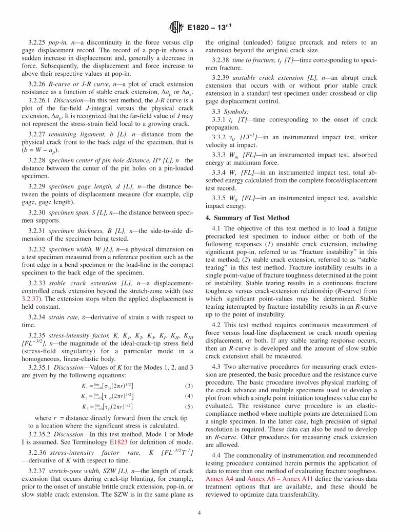
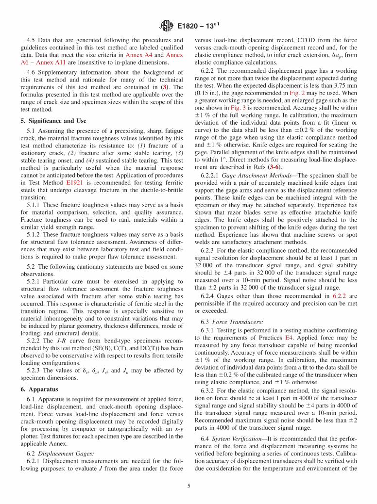
6.2.2 The recommended displacement gage has a workingrange of not more than twice the displacement expected duringthe test. When the expected displacement is less than 3.75 mm(0.15 in.), the gage recommended in Fig. 2 may be used. Whena greater working range is needed, an enlarged gage such as theone shown in Fig. 3 is recommended. Accuracy shall be within61 % of the full working range. In calibration, the maximumdeviation of the individual data points from a fit (linear orcurve) to the data shall be less than 60.2 % of the workingrange of the gage when using the elastic compliance methodand 61 % otherwise. Knife edges are required for seating thegage. Parallel alignment of the knife edges shall be maintainedto within 1°. Direct methods for measuring load-line displace-ment are described in Refs (3-6).

6.2.2.1 Gage Attachment Methods—The specimen shall beprovided with a pair of accurately machined knife edges thatsupport the gage arms and serve as the displacement referencepoints. These knife edges can be machined integral with thespecimen or they may be attached separately. Experience hasshown that razor blades serve as effective attachable knifeedges. The knife edges shall be positively attached to thespecimen to prevent shifting of the knife edges during the testmethod. Experience has shown that machine screws or spotwelds are satisfactory attachment methods.

6.2.3 For the elastic compliance method, the recommendedsignal resolution for displacement should be at least 1 part in32 000 of the transducer signal range, and signal stabilityshould be 64 parts in 32 000 of the transducer signal rangemeasured over a 10-min period. Signal noise should be lessthan 62 parts in 32 000 of the transducer signal range.

6.2.4 Gages other than those recommended in 6.2.2 arepermissible if the required accuracy and precision can be metor exceeded.

6.3 Force Transducers:6.3.1 Testing is performed in a testing machine conforming

to the requirements of Practices E4. Applied force may bemeasured by any force transducer capable of being recordedcontinuously. Accuracy of force measurements shall be within61 % of the working range. In calibration, the maximumdeviation of individual data points from a fit to the data shall beless than 60.2 % of the calibrated range of the transducer whenusing elastic compliance, and 61 % otherwise.

6.3.2 For the elastic compliance method, the signal resolu-tion on force should be at least 1 part in 4000 of the transducersignal range and signal stability should be 64 parts in 4000 ofthe transducer signal range measured over a 10-min period.Recommended maximum signal noise should be less than 62parts in 4000 of the transducer signal range.

6.4 System Verification—It is recommended that the perfor-mance of the force and displacement measuring systems beverified before beginning a series of continuous tests. Calibra-tion accuracy of displacement transducers shall be verified withdue consideration for the temperature and environment of the

E1820 − 13´1

5

test. Force calibrations shall be conducted periodically anddocumented in accordance with the latest revision of PracticesE4.

6.5 Fixtures:6.5.1 Bend-Test Fixture—The general principles of the

bend-test fixture are illustrated in Fig. 4. This fixture isdesigned to minimize frictional effects by allowing the supportrollers to rotate and move apart slightly as the specimen isloaded, thus permitting rolling contact. Thus, the supportrollers are allowed limited motion along plane surfaces parallelto the notched side of the specimen, but are initially positivelypositioned against stops that set the span length and are held in

FIG. 2 Double-Cantilever Clip-In Displacement Gage Mounted by Means of Integral Knife Edges

NOTE 1—All dimensions are in millimeters.FIG. 3 Clip Gage Design for 8.0 mm (0.3 in.)

and More Working Range

FIG. 4 Bend Test Fixture Design

E1820 − 13´1

6

place by low-tension springs (such as rubber bands). Fixturesand rolls shall be made of high hardness (greater than 40 HRC)steels.

6.5.2 Tension Testing Clevis:6.5.2.1 A loading clevis suitable for testing compact speci-

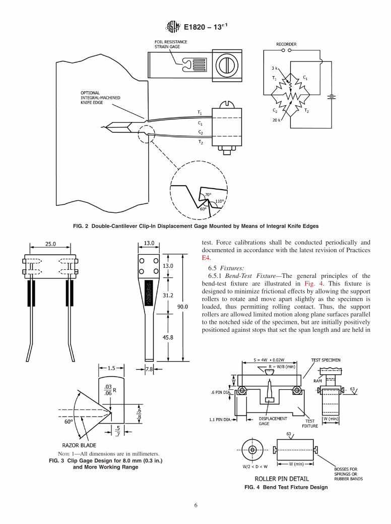
mens is shown in Fig. 5. Both ends of the specimen are held insuch a clevis and loaded through pins, in order to allow rotationof the specimen during testing. In order to provide rollingcontact between the loading pins and the clevis holes, theseholes are provided with small flats on the loading surfaces.Other clevis designs may be used if it can be demonstrated thatthey will accomplish the same result as the design shown.Clevises and pins should be fabricated from steels of sufficientstrength (greater than 40 HRC) to elastically resist indentationof the clevises or pins.

6.5.2.2 The critical tolerances and suggested proportions ofthe clevis and pins are given in Fig. 5. These proportions arebased on specimens having W/B = 2 for B > 12.7 mm (0.5 in.)and W/B = 4 for B ≤ 12.7 mm. If a 1930-MPa (280 000-psi)yield strength maraging steel is used for the clevis and pins,adequate strength will be obtained. If lower-strength gripmaterial is used, or if substantially larger specimens arerequired at a given σYS/E ratio, then heavier grips will berequired. As indicated in Fig. 5 the clevis corners may be cut

off sufficiently to accommodate seating of the clip gage inspecimens less than 9.5 mm (0.375 in.) thick.

6.5.2.3 Careful attention should be given to achieving goodalignment through careful machining of all auxiliary grippingfixtures.

7. Specimen Size, Configuration, and Preparation

7.1 Specimen Configurations—The configurations of thestandard specimens are shown in Annex A1 – Annex A3.

7.2 Crack Plane Orientation—The crack plane orientationshall be considered in preparing the test specimen. This isdiscussed in Terminology E1823.

7.3 Alternative Specimens—In certain cases, it may bedesirable to use specimens having W/B ratios other than two.Suggested alternative proportions for the single-edge bendspecimen are 1 ≤ W/B ≤ 4 and for the compact (and disk shapedcompact) specimen are 2 ≤ W/B ≤ 4. However, any thicknesscan be used as long as the qualification requirements are met.

7.4 Specimen Precracking—All specimens shall be pre-cracked in fatigue. Experience has shown that it is impracticalto obtain a reproducibly sharp, narrow machined notch thatwill simulate a natural crack well enough to provide asatisfactory fracture toughness test result. The most effective

NOTE 1—Corners may be removed as necessary to accommodate the clip gage.FIG. 5 Tension Testing Clevis Design

E1820 − 13´1

7

artifice for this purpose is a narrow notch from which extendsa comparatively short fatigue crack, called the precrack. (Afatigue precrack is produced by cyclically loading the notchedspecimen for a number of cycles usually between about 104

and 106 depending on specimen size, notch preparation, andstress intensity level.) The dimensions of the notch and theprecrack, and the sharpness of the precrack shall meet certainconditions that can be readily met with most engineeringmaterials since the fatigue cracking process can be closelycontrolled when careful attention is given to the knowncontributory factors. However, there are some materials thatare too brittle to be fatigue-cracked since they fracture as soonas the fatigue crack initiates; these are outside the scope of thepresent test method.

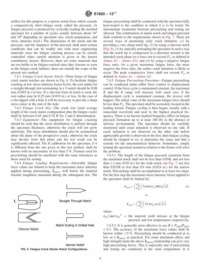
7.4.1 Fatigue Crack Starter Notch—Three forms of fatiguecrack starter notches are shown in Fig. 6. To facilitate fatiguecracking at low stress intensity factor levels, the root radius fora straight-through slot terminating in a V-notch should be 0.08mm (0.003 in.) or less. If a chevron form of notch is used, theroot radius may be 0.25 mm (0.010 in.) or less. In the case ofa slot tipped with a hole it will be necessary to provide a sharpstress raiser at the end of the hole.

7.4.2 Fatigue Crack Size—The crack size (total averagelength of the crack starter configuration plus the fatigue crack)shall be between 0.45 and 0.70 W for J and δ determination.

7.4.3 Equipment—The equipment for fatigue crackingshould be such that the stress distribution is uniform throughthe specimen thickness; otherwise the crack will not growuniformly. The stress distribution should also be symmetricalabout the plane of the prospective crack; otherwise the crackmay deviate from that plane and the test result can besignificantly affected. The K calibration for the specimen, if itis different from the one given in this test method, shall beknown with an uncertainty of less than 5 %. Fixtures used forprecracking should be machined with the same tolerances asthose used for testing.

7.4.4 Fatigue Loading Requirements—Allowable fatigueforce values are limited to keep the maximum stress intensityapplied during precracking, KMAX, well below the materialfracture toughness measured during the subsequent test. The

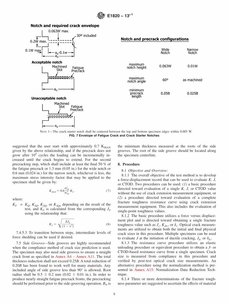
fatigue precracking shall be conducted with the specimen fullyheat-treated to the condition in which it is to be tested. Nointermediate treatments between precracking and testing areallowed. The combination of starter notch and fatigue precrackshall conform to the requirements shown in Fig. 7. There areseveral ways of promoting early crack initiation: (1) byproviding a very sharp notch tip, (2) by using a chevron notch(Fig. 6), (3) by statically preloading the specimen in such a waythat the notch tip is compressed in a direction normal to theintended crack plane (to a force not to exceed Pm as defined inAnnex A1 – Annex A3), and (4) by using a negative fatigueforce ratio; for a given maximum fatigue force, the morenegative the force ratio, the earlier crack initiation is likely tooccur. The peak compressive force shall not exceed Pm asdefined in Annex A1 – Annex A3.

7.4.5 Fatigue Precracking Procedure—Fatigue precrackingcan be conducted under either force control or displacementcontrol. If the force cycle is maintained constant, the maximumK and the K range will increase with crack size; if thedisplacement cycle is maintained constant, the reverse willhappen. The initial value of the maximum fatigue force shouldbe less than Pm. The specimen shall be accurately located in theloading fixture. Fatigue cycling is then begun, usually with asinusoidal waveform and near to the highest practical fre-quency. There is no known marked frequency effect on fatigueprecrack formation up to at least 100 Hz in the absence ofadverse environments. The specimen should be carefullymonitored until crack initiation is observed on one side. Ifcrack initiation is not observed on the other side beforeappreciable growth is observed on the first, then fatigue cyclingshould be stopped to try to determine the cause and find aremedy for the unsymmetrical behavior. Sometimes, simplyturning the specimen around in relation to the fixture will solvethe problem.

7.4.5.1 The length of the fatigue precrack extension fromthe machined notch shall not be less than 0.05B, and not lessthan 1.3 mm (0.05 in.) for the wide notch, see Fig. 7, nor lessthan 0.025B or less than 0.6 mm (0.024 in.) for the narrownotch. Precracking shall be accomplished in at least two steps.For the first step the maximum stress intensity factor applied tothe specimen shall be limited by:

KMAX 5 S σYSf

σYST D ~0.063σYS

f MPa=m! (6)

or

KMAX 5 S σYSf

σYST D ~0.4σYS

f ksi=in.!

where:σYS

f and σYST = the material yield stresses at the fatigue

precrack and test temperatures respectively.

7.4.5.2 It is generally most effective to use R = PMIN/PMAX

= 0.1. The accuracy of the maximum force values shall beknown within 65 %. Precracking should be conducted at aslow as a KMAX as practical. For some aluminum alloys andhigh strength steels the above KMAX relationship can give veryhigh precracking forces. This is especially true if precrackingand testing are conducted at the same temperature. It isFIG. 6 Fatigue Crack Starter Notch Configurations

E1820 − 13´1

8

suggested that the user start with approximately 0.7 KMAX

given by the above relationship, and if the precrack does notgrow after 105 cycles the loading can be incrementally in-creased until the crack begins to extend. For the secondprecracking step, which shall include at least the final 50 % ofthe fatigue precrack or 1.3 mm (0.05 in.) for the wide notch or0.6 mm (0.024 in.) for the narrow notch, whichever is less, themaximum stress intensity factor that may be applied to thespecimen shall be given by:

KMAX 5 0.6σYS

f

σYST KF (7)

where:KF = KQ, KJQ, KJQc or KJQu depending on the result of the

test, and KF is calculated from the corresponding JF

using the relationship that:

KF 5ΠEJF

~1 2 ν2!(8)

7.4.5.3 To transition between steps, intermediate levels offorce shedding can be used if desired.

7.5 Side Grooves—Side grooves are highly recommendedwhen the compliance method of crack size prediction is used.The specimen may also need side grooves to ensure a straightcrack front as specified in Annex A4 – Annex A11. The totalthickness reduction shall not exceed 0.25B. A total reduction of0.20B has been found to work well for many materials. Anyincluded angle of side groove less than 90° is allowed. Rootradius shall be 0.5 6 0.2 mm (0.02 6 0.01 in.). In order toproduce nearly straight fatigue precrack fronts, the precrackingshould be performed prior to the side-grooving operation. BN is

the minimum thickness measured at the roots of the sidegrooves. The root of the side groove should be located alongthe specimen centerline.

8. Procedure

8.1 Objective and Overview:8.1.1 The overall objective of the test method is to develop

a force-displacement record that can be used to evaluate K, J,or CTOD. Two procedures can be used: (1) a basic proceduredirected toward evaluation of a single K, J, or CTOD valuewithout the use of crack extension measurement equipment, or(2) a procedure directed toward evaluation of a completefracture toughness resistance curve using crack extensionmeasurement equipment. This also includes the evaluation ofsingle-point toughness values.

8.1.2 The basic procedure utilizes a force versus displace-ment plot and is directed toward obtaining a single fracturetoughness value such as Jc, KJIc, or δc. Optical crack measure-ments are utilized to obtain both the initial and final physicalcrack sizes in this procedure. Multiple specimens can be usedto evaluate J at the initiation of ductile cracking, JIc or δIc.

8.1.3 The resistance curve procedure utilizes an elasticunloading procedure or equivalent procedure to obtain a J- orCTOD-based resistance curve from a single specimen. Cracksize is measured from compliance in this procedure andverified by post-test optical crack size measurements. Analternative procedure using the normalization method is pre-sented in Annex A15: Normalization Data Reduction Tech-nique.

8.1.4 Three or more determinations of the fracture tough-ness parameter are suggested to ascertain the effects of material

NOTE 1—The crack-starter notch shall be centered between the top and bottom specimen edges within 0.005 W.FIG. 7 Envelope of Fatigue Crack and Crack Starter Notches

E1820 − 13´1

9

and test system variability. If fracture occurs by cleavage offerritic steel, the testing and analysis procedures of TestMethod E1921 are recommended.

8.2 System and Specimen Preparation:8.2.1 Specimen Measurement—Measure the dimensions,

BN, B, W, H*, and d to the nearest 0.050 mm (0.002 in.) or0.5 %, whichever is larger.

8.2.2 Specimen Temperature:8.2.2.1 The temperature of the specimen shall be stable and

uniform during the test. Hold the specimen at test temperature63 °C for 1⁄2 h/25 mm of specimen thickness.

8.2.2.2 Measure the temperature of the specimen during thetest to an accuracy of 63 °C, where the temperature ismeasured on the specimen surface within W/4 from the cracktip. (See Test Methods E21 for suggestions on temperaturemeasurement.)

8.2.2.3 For the duration of the test, the difference betweenthe indicated temperature and the nominal test temperatureshall not exceed 63 °C.

8.2.2.4 The term “indicated temperature” means the tem-perature that is indicated by the temperature measuring deviceusing good-quality pyrometric practice.

NOTE 3—It is recognized that specimen temperature may vary morethan the indicated temperature. The permissible indicated temperaturevariations in 8.2.2.3 are not to be construed as minimizing the importanceof good pyrometric practice and precise temperature control. All labora-tories should keep both indicated and specimen temperature variations assmall as practicable. It is well recognized, in view of the dependency offracture toughness of materials on temperature, that close temperaturecontrol is necessary. The limits prescribed represent ranges that arecommon practice.

8.3 Alignment:8.3.1 Bend Testing—Set up the bend test fixture so that the

line of action of the applied force passes midway between thesupport roll centers within 61 % of the distance between thecenters. Measure the span to within 60.5 % of the nominallength. Locate the specimen so that the crack tip is midwaybetween the rolls to within 1 % of the span and square to rollaxes within 62°.

8.3.1.1 When the load-line displacement is referenced fromthe loading jig, there is potential for introduction of error fromtwo sources. They are the elastic compression of the fixture asthe force increases and indentation of the specimen at theloading points. Direct methods for load-line displacementmeasurement are described in Refs (4-7). If a remote trans-ducer is used for load-line displacement measurement, takecare to exclude the elastic displacement of the load-trainmeasurement and brinelling displacements at the load points(8).

8.3.2 Compact Testing—Loading pin friction and eccentric-ity of loading can lead to errors in fracture toughness determi-nation. The centerline of the upper and lower loading rodsshould be coincident within 0.25 mm (0.01 in.). Center thespecimen with respect to the clevis opening within 0.76 mm(0.03 in.). Seat the displacement gage in the knife edges firmlyby wiggling the gage lightly.

8.4 Basic Procedure—Load all specimens under displace-ment gage or machine crosshead or actuator displacement

control. If a loading rate that exceeds that specified here isdesired, please refer to Annex A14: Special Requirements forRapid-Load J-Integral Fracture Toughness Testing.

8.4.1 The basic procedure involves loading a specimen to aselected displacement level and determining the amount ofcrack extension that occurred during loading.

8.4.2 Load specimens at a constant rate such that the timetaken to reach the force Pm, as defined in Annex A1 – AnnexA3, lies between 0.3 to 3 min.

8.4.3 If the test ends by fracture instability, measure theinitial crack size and any ductile crack extension by theprocedure in 9. Ductile crack extension may be difficult todistinguish but should be defined on one side by the fatigueprecrack and on the other by the brittle region. Proceed to 9 toevaluate fracture toughness in terms of K, J, or CTOD.

8.4.4 If stable tearing occurs, test additional specimens toevaluate an initiation value of the toughness. Use the procedurein 8.5 to evaluate the amount of stable tearing that has occurredand thus determine the displacement levels needed in theadditional tests. Five or more points favorably positioned arerequired to generate an R curve for evaluating an initiationpoint. See Annex A9 and Annex A11 to see how points shall bepositioned for evaluating an initiation toughness value.

8.5 Optical Crack Size Measurement:8.5.1 After unloading the specimen, mark the crack accord-

ing to one of the following methods. For steels and titaniumalloys, heat tinting at about 300 °C (570 °F) for 30 min workswell. For other materials, fatigue cycling can be used. The useof liquid penetrants is not recommended. For both recom-mended methods, the beginning of stable crack extension ismarked by the end of the flat fatigue precracked area. The endof crack extension is marked by the end of heat tint or thebeginning of the second flat fatigue area.

8.5.2 Break the specimen to expose the crack, with caretaken to minimize additional deformation. Cooling ferritic steelspecimens to ensure brittle behavior may be helpful. Coolingnonferritic materials may help to minimize deformation duringfinal fracture.

8.5.3 Along the front of the fatigue crack and the front of themarked region of stable crack extension, measure the size ofthe original crack and the final physical crack size at nineequally spaced points centered about the specimen centerlineand extending to 0.005 W from the root of the side groove orsurface of plane-sided specimens. Calculate the original cracksize, ao, and the final physical crack size, ap, as follows:average the two near-surface measurements, combine the resultwith the remaining seven crack size measurements and deter-mine the average. Calculate the physical crack extension, ∆ap

= ap − ao. The measuring instrument shall have an accuracy of0.025 mm (0.001 in.).

8.5.4 None of the nine measurements of original crack sizeand final physical crack size may differ by more than 0.05Bfrom the average physical crack size defined in 8.5.3.

8.6 Resistance Curve Procedure:8.6.1 The resistance curve procedure involves using an

elastic compliance technique or other technique to obtain the Jor CTOD resistance curve from a single specimen test. The

E1820 − 13´1

10

elastic compliance technique is described here, while thenormalization technique is described in Annex A15.

8.6.2 Load the specimens under displacement gage or ma-chine crosshead or actuator displacement control. Load thespecimens at a rate such that the time taken to reach the forceP m, as defined in Annex A1 – Annex A3, lies between 0.3 and3.0 min. The time to perform an unload/reload sequence shouldbe as needed to accurately estimate crack size, but not morethan 10 min. If a higher loading rate is desired, please refer toAnnex A14: Special Requirements for Rapid-Load J-IntegralFracture Toughness Testing.

8.6.3 Take each specimen individually through the follow-ing steps:

8.6.3.1 Measure compliance to estimate the original cracksize, ao, using unloading/reloading sequences in a force rangefrom 0.5 to 1.0 times the maximum precracking force. Estimatea provisional initial crack size, aoq, from at least threeunloading/reloading sequences. No individual value shall differfrom the mean by more than 60.002 W.

8.6.3.2 Proceed with the test using unload/reload sequencesthat produce crack extension measurements at intervals pre-scribed by the applicable data analysis section of Annex A8 orAnnex A10. Note that at least eight data points are requiredbefore specimen achieves maximum force. If crack size valueschange negatively by more than 0.005 ao (backup), stop the testand check the alignment of the loading train. Crack size valuesdetermined at forces lower than the maximum precrackingforce should be ignored.

8.6.3.3 For many materials, load relaxation may occur priorto conducting compliance measurements, causing a time-dependent nonlinearity in the unloading slope. One methodthat may be used to remedy this effect is to hold the specimenfor a period of time until the force becomes stable at a constantdisplacement prior to initiating the unloading.

8.6.3.4 The maximum recommended range of unload/reloadfor crack extension measurement should not exceed either50 % of Pm, as defined in Annex A1 – Annex A3, or 50 % ofthe current force, whichever is smaller.

8.6.3.5 After completing the final unloading cycle, returnthe force to zero without additional crosshead displacementbeyond the then current maximum displacement.

8.6.3.6 After unloading the specimen, use the procedure in8.5 to optically measure the crack sizes.

8.7 Alternative Methods:8.7.1 Alternative methods of measuring crack extension,

such as the electric potential drop method, are allowed.Methods shall meet the qualification criteria given in 9.1.5.2. Ifan alternative method is used to obtain JIc, at least oneadditional, confirmatory specimen shall be tested at the sametest rate and under the same test conditions. From the alterna-tive method the load-line displacement corresponding to aductile crack extension of 0.5 mm shall be estimated. Theadditional specimen shall then be loaded to this load-linedisplacement level, marked, broken open and the ductile crackgrowth measured. The measured crack extension shall be 0.5 6

0.25 mm in order for these results, and hence the JIc value, tobe qualified according to this method.

8.7.2 If displacement measurements are made in a planeother than that containing the load-line, the ability to inferload-line displacement shall be demonstrated using the testmaterial under similar test temperatures and conditions. In-ferred load-line displacement values shall be accurate to within61 %.

9. Analysis of Results

9.1 Qualification of Data—The data shall meet the follow-ing requirements to be qualified according to this test method.If the data do not pass these requirements, no fracture tough-ness measures can be determined in accordance with this testmethod.

NOTE 4—This section contains the requirements for qualification thatare common for all tests. Additional qualification requirements are givenwith each type of test in the Annexes as well as requirements fordetermining whether the fracture toughness parameter developed isinsensitive to in-plane dimensions.

9.1.1 All requirements on the test equipment in Section 6shall be met.

9.1.2 All requirements on machining tolerance and pre-cracking in Section 7 shall be met.

9.1.3 All requirements on fixture alignment, test rate, andtemperature stability and accuracy in Section 8 shall be met.

9.1.4 The following crack size requirements shall be met inall tests.

9.1.4.1 Original Crack Size—None of the nine physicalmeasurements of initial crack size defined in 8.5.3 shall differby more than 0.05B from the average ao.

9.1.4.2 Final Crack Size—None of the nine physical mea-surements of final physical crack size, ap, defined in 8.5.3 shalldiffer by more than 0.05B from the average ap. In subsequenttests, the side-groove configuration may be modified within therequirements of 7.5 to facilitate meeting this requirement.

9.1.5 The following crack size requirements shall be met inthe tests using the resistance curve procedure of 8.6.

9.1.5.1 Crack Extension—None of the nine physical mea-surements of crack extension shall be less than 50 % of theaverage crack extension.

9.1.5.2 Crack Extension Prediction—The crack extension,∆apredicted, predicted from elastic compliance (or othermethod), at the last unloading shall be compared with themeasured physical crack extension, ∆ap. The difference be-tween these shall not exceed 0.15 ∆ ap for crack extensions lessthan 0.2 bo, and the difference shall not exceed 0.03 bo

thereafter.

9.2 Fracture Instability—When the test terminates withfracture instability, evaluate whether the fracture occurredbefore stable tearing or after stable tearing. The beginning ofstable tearing is defined in A6.3 and A7.3. For fractureinstability occurring before stable tearing proceed to AnnexA6, and Annex A7 to evaluate the toughness values in terms ofK, J, or CTOD. For fracture instability occurring after stabletearing, proceed to Annex A6, and Annex A7 to evaluatetoughness values and then go to 9.3 to evaluate stable tearing.

9.3 Stable Tearing:

E1820 − 13´1

11

9.3.1 Basic Procedure—When the basic procedure is used,only an initiation toughness can be evaluated. Proceed toAnnex A9 and Annex A11 to evaluate initiation toughnessvalues.

9.3.2 Resistance Curve Procedure—When the resistancecurve procedure is used, refer to Annex A8 and Annex A10 todevelop the R-curves. Proceed to Annex A9 and Annex A11 todevelop initiation values of toughness.

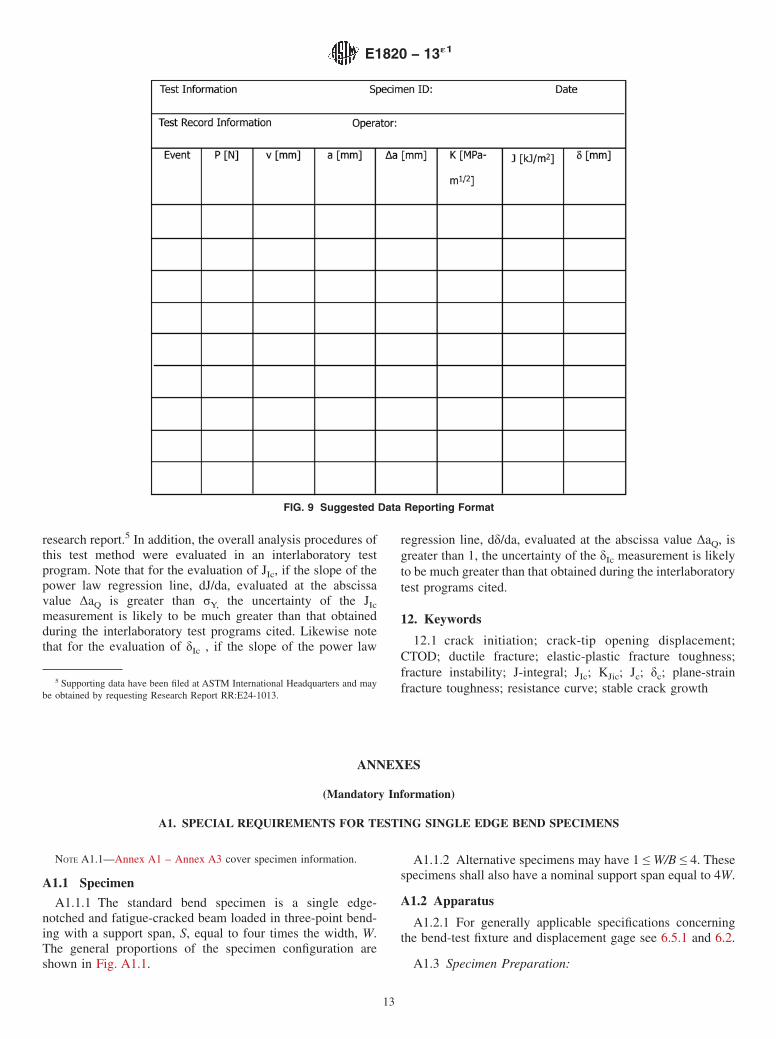
10. Report

10.1 Recommended tables for reporting results are given inFig. 8 and Fig. 9.

10.2 Report the following information for each fracturetoughness determination:

10.2.1 Type of test specimen and orientation of test speci-men according to Terminology E1823 identification codes,

10.2.2 Material designation (ASTM, AISI, SAE, and soforth), material product form (plate, forging, casting, and soforth), and material yield and tensile strength (at testtemperature),

10.2.3 Specimen dimensions (8.2.1), thickness B and BN,and width W,

10.2.4 Test temperature (8.2.2), loading rate (8.4.2 and8.6.2), and type of loading control,

10.2.5 Fatigue precracking conditions (7.4), Kmax, ∆Krange, and fatigue precrack size (average),

10.2.6 Load-displacement record and associated calcula-tions (Section 9),

10.2.7 If the loading rate is other than quasi-static, report theapplied dK/dt,

10.2.8 Original measured crack size, ao (8.5), originalpredicted crack size, aoq , final measured crack size, ap, finalpredicted crack extension, ∆apredicted, physical crack extensionduring test, ∆ap, crack front appearance—straightness andplanarity, and fracture appearance,

10.2.9 Qualification of fracture toughness measurement(Annex A4 and Annex A6 – Annex A11), based on sizerequirements, and based on crack extension, and

10.2.10 Qualified values of fracture toughness, includingR-curve values.

11. Precision and Bias

11.1 Bias—There is no accepted “standard” value for any ofthe fracture toughness criteria employed in this test method. Inthe absence of such a true value no meaningful statement canbe made concerning bias of data.

11.2 Precision—The precision of any of the various fracturetoughness determinations cited in this test method is a functionof the precision and bias of the various measurements of lineardimensions of the specimen and testing fixtures, the precisionof the displacement measurement, the bias of the force mea-surement as well as the bias of the recording devices used toproduce the force-displacement record, and the precision of theconstructions made on this record. It is not possible to makemeaningful statements concerning precision and bias for allthese measurements. However, it is possible to derive usefulinformation concerning the precision of fracture toughnessmeasurements in a global sense from interlaboratory test

programs. Most of the measures of fracture toughness that canbe determined by this procedure have been evaluated by aninterlaboratory test program. The JIc was evaluated in (9), theJ-R curve was evaluated in (10), and δc was evaluated in a

Basic Test InformationLoading Rate, time to Pm = [min]Test temperature = [°C]

Crack Size InformationInitial measured crack size, ao = [mm]Initial predicted crack size, aoq = [mm]Final measured crack size, af = [mm]Final ∆ap = [mm]Final ∆apredicted = [mm]

Analysis of ResultsFracture type = (Fracture instability or stable tearing)

K Based FractureKJIc = [MPa-m1/2]

J Based FractureJc = [kJ/m2]JIc = [kJ/m2]Ju = [kJ/m2]

δ Based Resultsδc

* = [mm]δIc = [mm]δc = [mm]δu = [mm]

Final ∆a/b =Final Jmax/σYS = [mm]

Specimen InformationType =Identification =Orientation =

Basic dimensionsB = [mm]BN = [mm]W = [mm]aN(Notch Length) = [mm]

Particular dimensionsC(T) H = [mm]SE(B) S = [mm]DC(T) D = [mm]

MaterialMaterial designation =Form =

Tensile PropertiesE (Young’s modulus) = [MPa]ν (Poisson’s ratio) =σYS (Yield Strength) = [MPa]σTS (Ultimate Strength) = [MPa]

Precracking InformationFinal Pmax = [N]Final Pmin = [N]Pm = [N]Final ∆K/E = [MPa-m1/2]Fatigue temperature = [°C]Fatigue crack growth information

FIG. 8 Suggested Data Reporting Format

E1820 − 13´1

12

research report.5 In addition, the overall analysis procedures ofthis test method were evaluated in an interlaboratory testprogram. Note that for the evaluation of JIc, if the slope of thepower law regression line, dJ/da, evaluated at the abscissavalue ∆aQ is greater than σY, the uncertainty of the JIc

measurement is likely to be much greater than that obtainedduring the interlaboratory test programs cited. Likewise notethat for the evaluation of δIc , if the slope of the power law

regression line, dδ/da, evaluated at the abscissa value ∆aQ, isgreater than 1, the uncertainty of the δIc measurement is likelyto be much greater than that obtained during the interlaboratorytest programs cited.

12. Keywords

12.1 crack initiation; crack-tip opening displacement;CTOD; ductile fracture; elastic-plastic fracture toughness;fracture instability; J-integral; JIc; KJic; Jc; δc; plane-strainfracture toughness; resistance curve; stable crack growth

ANNEXES

(Mandatory Information)

A1. SPECIAL REQUIREMENTS FOR TESTING SINGLE EDGE BEND SPECIMENS

NOTE A1.1—Annex A1 – Annex A3 cover specimen information.

A1.1 Specimen

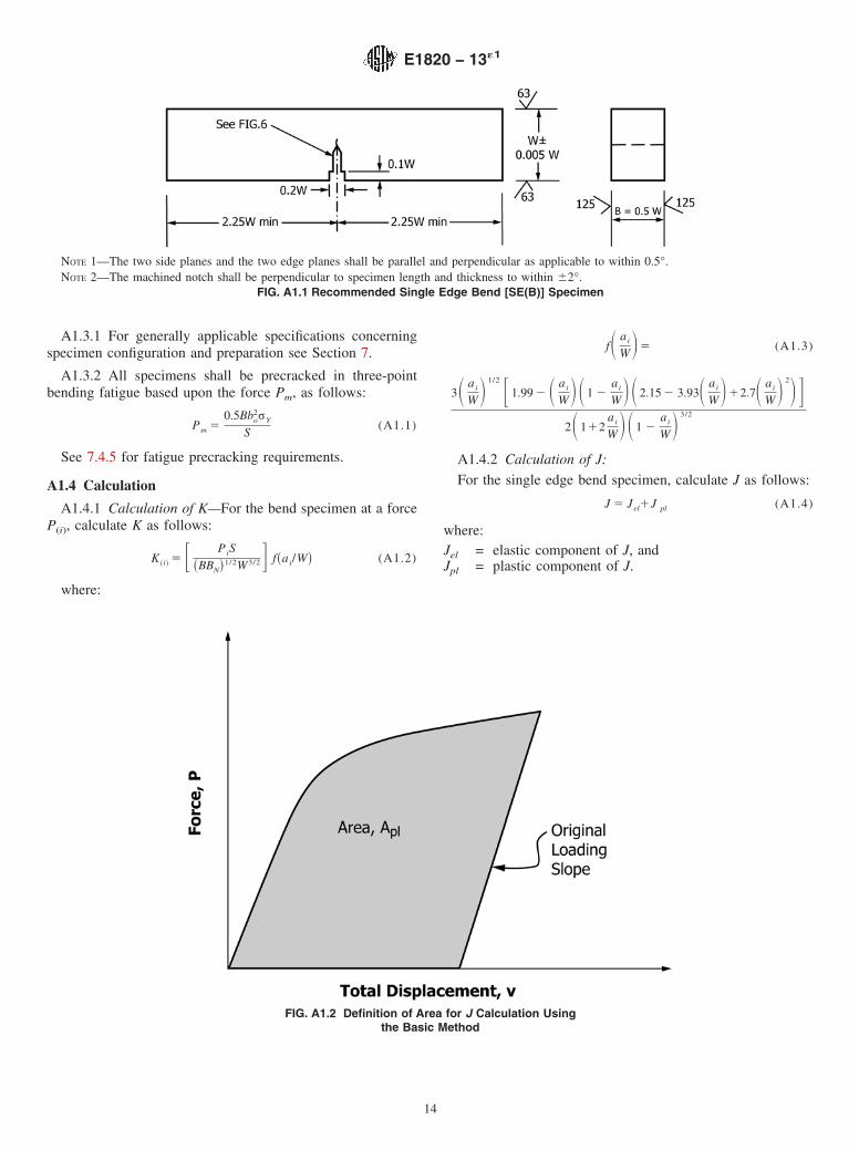
A1.1.1 The standard bend specimen is a single edge-notched and fatigue-cracked beam loaded in three-point bend-ing with a support span, S, equal to four times the width, W.The general proportions of the specimen configuration areshown in Fig. A1.1.

A1.1.2 Alternative specimens may have 1 ≤ W/B ≤ 4. Thesespecimens shall also have a nominal support span equal to 4W.

A1.2 Apparatus

A1.2.1 For generally applicable specifications concerningthe bend-test fixture and displacement gage see 6.5.1 and 6.2.

A1.3 Specimen Preparation:

5 Supporting data have been filed at ASTM International Headquarters and maybe obtained by requesting Research Report RR:E24-1013.

FIG. 9 Suggested Data Reporting Format

E1820 − 13´1

13

A1.3.1 For generally applicable specifications concerningspecimen configuration and preparation see Section 7.

A1.3.2 All specimens shall be precracked in three-pointbending fatigue based upon the force Pm, as follows:

Pm 50.5Bbo

2σY

S(A1.1)

See 7.4.5 for fatigue precracking requirements.

A1.4 Calculation

A1.4.1 Calculation of K—For the bend specimen at a forceP(i), calculate K as follows:

K~i!

5 F PiS

~BBN!1/2W3/2G f~ai/W! (A1.2)

where:

fS ai

W D5 (A1.3)

3S ai

W D 1/2 F 1.99 2 S ai

W D S 1 2ai

W D S 2.15 2 3.93S ai

W D12.7S ai

W D 2D G2S 112

ai

W D S 1 2ai

W D 3/2

A1.4.2 Calculation of J:

For the single edge bend specimen, calculate J as follows:

J 5 Jel1J pl (A1.4)

where:Jel = elastic component of J, andJpl = plastic component of J.

NOTE 1—The two side planes and the two edge planes shall be parallel and perpendicular as applicable to within 0.5°.NOTE 2—The machined notch shall be perpendicular to specimen length and thickness to within 62°.

FIG. A1.1 Recommended Single Edge Bend [SE(B)] Specimen

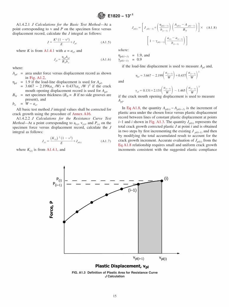
FIG. A1.2 Definition of Area for J Calculation Usingthe Basic Method

E1820 − 13´1

14

A1.4.2.1 J Calculations for the Basic Test Method—At apoint corresponding to v and P on the specimen force versusdisplacement record, calculate the J integral as follows:

J 5K2 ~1 2 ν2!

E1Jpl (A1.5)

where K is from A1.4.1 with a = ao, and

Jpl 5ηplApl

BNbo

(A1.6)

where:Apl = area under force versus displacement record as shown

in Fig. A1.2,ηpl = 1.9 if the load-line displacement is used for Apl,

= 3.667 − 2.199(ao /W) + 0.437(ao /W )2 if the crackmouth opening displacement record is used for Apl,

BN = net specimen thickness (BN = B if no side grooves arepresent), and

bo = W − ao.

All basic test method J integral values shall be corrected forcrack growth using the procedure of Annex A16.

A1.4.2.2 J Calculations for the Resistance Curve TestMethod—At a point corresponding to a(i), v(i), and P(i) on thespecimen force versus displacement record, calculate the Jintegral as follows:

J~i!

5~K

~i!!2 ~1 2 v2!

E1Jpl~i!

(A1.7)

where K(i) is from A1.4.1, and

Jpl~i!5 F J pl~i21!

1S ηpl~i21!

b~i21!

D S Apl~i!2 A pl~i21!

BND G3 (A1.8)

F 1 2 γpl~i21!S a~i!

2 a~i21!

b~i21!

D Gwhere:ηpl(i−1) = 1.9, andγpl(i−1) = 0.9

if the load-line displacement is used to measure Apl and,

ηpl 5 3.667 2 2.199S a~i21!

W D10.437S a~i21!

W D 2

and

γpl 5 0.13112.131S a~i21!

W D 2 1.465 S a~i21!

W D 2

if the crack mouth opening displacement is used to measureApl.

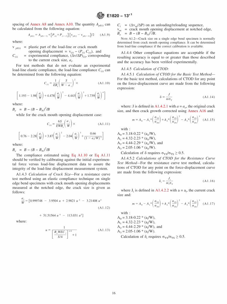
In Eq A1.8, the quantity Apl(i) − Apl(i–1) is the increment ofplastic area under the chosen force versus plastic displacementrecord between lines of constant plastic displacement at pointsi−1 and i shown in Fig. A1.3. The quantity Jpl(i) represents thetotal crack growth corrected plastic J at point i and is obtainedin two steps by first incrementing the existing J pl(i-1) and thenby modifying the total accumulated result to account for thecrack growth increment. Accurate evaluation of Jpl(i) from theEq A1.8 relationship requires small and uniform crack growthincrements consistent with the suggested elastic compliance

FIG. A1.3 Definition of Plastic Area for Resistance CurveJ Calculation

E1820 − 13´1

15

spacing of Annex A8 and Annex A10. The quantity Apl(i) canbe calculated from the following equation:

Apl~i!5 Apl~i21!

1@P~i!

1P~i21!# @vpl~i!

2 vpl~i21!#/2 (A1.9)

where:v pl(i) = plastic part of the load-line or crack mouth

opening displacement = v(i) − (P(i) C(i)), andC(i) = experimental compliance, (∆v/∆P)(i), corresponding

to the current crack size, ai.

For test methods that do not evaluate an experimentalload-line elastic compliance, the load-line compliance C(i) canbe determined from the following equation:

C~i!

51

EBeS S

W 2 a iD 2

3 (A1.10)

F 1.193 2 1.98S ai

W D14.478S ai

W D 2

2 4.443S ai

W D 3

11.739S ai

W D 4Gwhere:Be = B − (B − BN)2/B

while for the crack mouth opening displacement case:

C~i!

56S

EWBeS a i

W D3 (A1.11)

F 0.76 2 2.28S ai

W D13.87S ai

W D 2

2 2.04S ai

W D 3

10.66

~1 2 ai/W! 2Gwhere:Be = B − (B − BN)2/B

The compliance estimated using Eq A1.10 or Eq A1.11should be verified by calibrating against the initial experimen-tal force versus load-line displacement data to assure theintegrity of the load-line displacement measurement system.

A1.4.3 Calculation of Crack Size—For a resistance curvetest method using an elastic compliance technique on singleedge bend specimens with crack mouth opening displacementsmeasured at the notched edge, the crack size is given asfollows:

ai

W5 @0.999748 2 3.9504 u 1 2.9821 u 2 2 3.21408 u3

(A1.12)

1 51.51564 u 4 2 113.031 u5#

where:

u 51

F BeWEC i

S/4 G 1/2

11

(A1.13)

Ci = (∆vm/∆P) on an unloading/reloading sequence,vm = crack mouth opening displacement at notched edge,Be = B − (B − BN)2/B.

NOTE A1.2—Crack size on a single edge bend specimen is normallydetermined from crack mouth opening compliance. It can be determinedfrom load-line compliance if the correct calibration is available.

A1.4.4 Other compliance equations are acceptable if theresulting accuracy is equal to or greater than those describedand the accuracy has been verified experimentally.

A1.4.5 Calculation of CTOD:

A1.4.5.1 Calculation of CTOD for the Basic Test Method—For the basic test method, calculations of CTOD for any pointon the force-displacement curve are made from the followingexpression:

δ 5J

mσY

(A1.14)

where: J is defined in A1.4.2.1 with a = ao, the original cracksize, and then crack growth corrected using Annex A16 and:

m 5 A0 2 A1*S σYS

σTSD1A2*S σYS

σTSD 2

2 A3*S σYS

σTSD 3

(A1.15)

with :A0 = 3.18-0.22 * (ao/W),A1 = 4.32-2.23 * (ao/W),A2 = 4.44-2.29 * (ao/W), andA3 = 2.05-1.06 * (ao/W).

Calculation of δ requires σYS/σTS ≥ 0.5.A1.4.5.2 Calculations of CTOD for the Resistance Curve

Test Method—For the resistance curve test method, calcula-tions of CTOD for any point on the force-displacement curveare made from the following expression:

δ i 5Ji

miσY

(A1.16)

where Ji is defined in A1.4.2.2 with a = ai, the current cracksize and:

m 5 A0 2 A1*S σYS

σTSD1A2*S σYS

σTSD 2

2 A3*S σYS

σTSD 3

(A1.17)

with :A0 = 3.18-0.22 * (ai/W),A1 = 4.32-2.23 * (ai/W),A2 = 4.44-2.29 * (ai/W), andA3 = 2.05-1.06 * (ai/W).

Calculation of δi requires σYS/σTS ≥ 0.5.

E1820 − 13´1

16

A2. SPECIAL REQUIREMENTS FOR TESTING COMPACT SPECIMENS

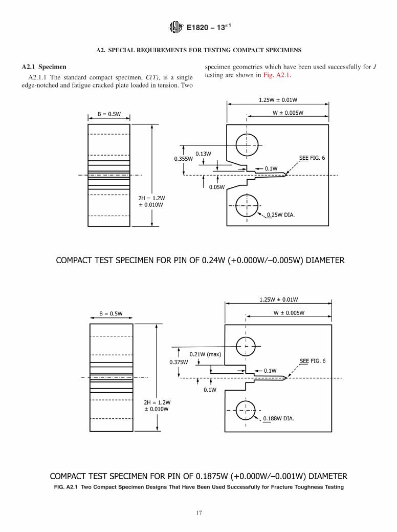
A2.1 Specimen

A2.1.1 The standard compact specimen, C(T), is a singleedge-notched and fatigue cracked plate loaded in tension. Two

specimen geometries which have been used successfully for Jtesting are shown in Fig. A2.1.

FIG. A2.1 Two Compact Specimen Designs That Have Been Used Successfully for Fracture Toughness Testing

E1820 − 13´1

17

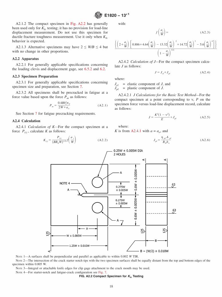
A2.1.2 The compact specimen in Fig. A2.2 has generallybeen used only for KIc testing; it has no provision for load-linedisplacement measurement. Do not use this specimen forductile fracture toughness measurement. Use it only when KIc

behavior is expected.

A2.1.3 Alternative specimens may have 2 ≤ W/B ≤ 4 butwith no change in other proportions.

A2.2 Apparatus

A2.2.1 For generally applicable specifications concerningthe loading clevis and displacement gage, see 6.5.2 and 6.2.

A2.3 Specimen Preparation

A2.3.1 For generally applicable specifications concerningspecimen size and preparation, see Section 7.

A2.3.2 All specimens shall be precracked in fatigue at aforce value based upon the force Pm as follows:

Pm 50.4Bbo

2σY

2W1ao

(A2.1)

See Section 7 for fatigue precracking requirements.

A2.4 Calculation

A2.4.1 Calculation of K—For the compact specimen at aforce P(i) , calculate K as follows:

K~i!

5P

~i!

~BBNW!1/2 fS a i

W D (A2.2)

with:

f S ai

W D5 (A2.3)

H S 21ai

W D F 0.88614.64S ai

W D 2 13.32S ai

W D 2

114.72S ai

W D 3

2 5.6S ai

W D 4G JS 1 2

ai

W D 3/2

A2.4.2 Calculation of J—For the compact specimen calcu-late J as follows:

J 5 Jel1Jpl (A2.4)

where:Jel = elastic component of J, andJpl = plastic component of J.

A2.4.2.1 J Calculations for the Basic Test Method—For thecompact specimen at a point corresponding to ν, P on thespecimen force versus load-line displacement record, calculateas follows:

J 5K2~1 2 ν2!

E1Jpl (A2.5)

where:K is from A2.4.1 with a = ao, and

Jpl 5η pl A pl

BNbo

(A2.6)

NOTE 1—A surfaces shall be perpendicular and parallel as applicable to within 0.002 W TIR.NOTE 2—The intersection of the crack starter notch tips with the two specimen surfaces shall be equally distant from the top and bottom edges of the

specimen within 0.005 W.NOTE 3—Integral or attachable knife edges for clip gage attachment to the crack mouth may be used.NOTE 4—For starter-notch and fatigue-crack configuration see Fig. 7.

FIG. A2.2 Compact Specimen for KIc Testing

E1820 − 13´1

18

where:Apl = area shown in Fig. A1.2,BN = net specimen thickness (BN = B if no side grooves are

present),bo = uncracked ligament, (W − ao), andηpl = 2 + 0.522bo/W.

All basic test method J integral values shall be corrected forcrack growth using the procedure of Annex A16.

A2.4.2.2 J Calculation for the Resistance Curve TestMethod—For the C(T) specimen at a point corresponding a (i),v(i), and P(i) on the specimen force versus load-line displace-ment record calculate as follows:

J~i!

5~K

~i!!2 ~1 2 ν2!

E1J pl~i!

(A2.7)

where K(i) is from A2.4.1, and:

J pl~i!5 (A2.8)

F Jpl ~i21!1S ηpl ~i21!

b~i21!

D Apl~i!2 Apl~i21!

BNG F 1 2 γ

~i21! S a~i!

2 a~i21!

b~i21!

D Gwhere:ηpl (i –1) = 2.0 + 0.522 b(i−1)/W, andγ(i –1) = 1.0 + 0.76 b(i−1)/W.

In Eq A2.8, the quantity Apl(i) − Apl(i-1) is the increment ofplastic area under the force versus plastic load-line displace-ment record between lines of constant displacement at pointsi−1 and i shown in Fig. A1.3. The quantity Jpl(i) represents thetotal crack growth corrected plastic J at point i and is obtainedin two steps by first incrementing the existing Jpl(i−1) and thenby modifying the total accumulated result to account for thecrack growth increment. Accurate evaluation of J pl(i) from theabove relationship requires small and uniform crack growthincrements consistent with the suggested elastic compliancespacing of Annex A8 and Annex A10. The quantity A pl(i) canbe calculated from the following equation:

Apl~i!5 Apl~i21!

1@P

~i!1P

~i21!# @ vpl~i!2 v pl~i21!#

2(A2.9)

where:vpl(i) = plastic part of the load-line displacement,

vi − P(i)CLL(i) , andCLL(i) = experimental compliance, (∆v/∆P)i, corresponding

to the current crack size, ai.

For test methods that do not evaluate an experimental elasticcompliance, CLL(i) can be determined from the followingequation:

CLL~i!5

1EBe

S W1ai

W 2 a iD 2 F 2.1630112.219S a i

W D 2 20.065S a i

W D 2

2 0.9925S a i

W D 3

120.609S a i

W D 4

2 9.9314S a i

W D 5G (A2.10)

where:

Be 5 B 2~B 2 BN!2

B(A2.11)

The load-line compliance estimated using Eq A2.10 shouldbe verified by calibrating against the initial experimentalcompliance to assure the integrity of the load-line displacementmeasurement system.

In an elastic compliance test, the rotation correctedcompliance, Cc(i), described in A2.4.4 shall be used instead ofCLL(i) in Eq A2.10.

A2.4.3 Calculation of Crack Size—For a single specimentest method using an elastic compliance technique on thecompact specimen with crack opening displacements measuredon the load-line, the crack size is given as follows:

ai/W 5 1.000196 2 4.06319u111.242u 2 2 106.043u31464.335u 4

2 650.677u5 (A2.12)

where:

u 51

@BeECc~i!#1/211

(A2.13)

Cc(i) = specimen load-line crack opening elastic compliance(∆v/∆P) on an unloading/reloading sequence cor-rected for rotation (see A2.4.4),

Be = B − (B − BN)2/B.

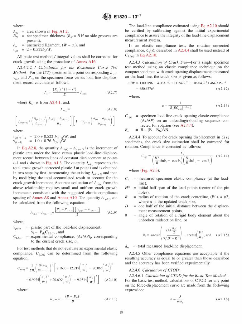
A2.4.4 To account for crack opening displacement in C(T)specimens, the crack size estimation shall be corrected forrotation. Compliance is corrected as follows:

Cc~i!5

Ci

S H*R

sinθ i 2 cos θ iD S DR

sinθ i 2 cos θ iD (A2.14)

where (Fig. A2.3):

Ci = measured specimen elastic compliance (at the load-line),

H* = initial half-span of the load points (center of the pinholes),

R = radius of rotation of the crack centerline, (W + a )/2,where a is the updated crack size,

D = one half of the initial distance between the displace-ment measurement points,

θ = angle of rotation of a rigid body element about theunbroken midsection line, or

θ i 5 arcsin1 D1dm

2

=D21R 22 2 arctanS DR D , and (A2.15)

dm = total measured load-line displacement.

A2.4.5 Other compliance equations are acceptable if theresulting accuracy is equal to or greater than those describedand the accuracy has been verified experimentally.

A2.4.6 Calculation of CTOD:A2.4.6.1 Calculation of CTOD for the Basic Test Method—

For the basic test method, calculations of CTOD for any pointon the force-displacement curve are made from the followingexpression:

δ 5J

mσY

(A2.16)

E1820 − 13´1

19

where J is defined in A2.4.2.1 with a = ao, the original cracksize, and then crack growth corrected using Annex A16 and:

m 5 A0 2 A1*S σYS

σTSD1A2*S σYS

σTSD 2

2 A3*S σYS

σTSD 3

(A2.17)

with: A0=3.62, A1 = 4.21, A2=4.33, and A3=2.00. Calcula-tion of δ requires σYS/σTS ≥ 0.5.

A2.4.6.2 Calculation of CTOD for the Resistance CurveTest Method—For the resistance curve test method, calcula-tions of CTOD for any point on the force-displacement curveare made from the following expression:

δ i 5Ji

mσY

(A2.18)

where J is defined in A2.4.2.2 with a = ai, the current cracksize, and,

m 5 A0 2 A1*S σYS

σTSD1A2*S σYS

σTSD 2

2 A3*S σYS

σTSD 3

(A2.19)

with: A0=3.62, A1 = 4.21, A2=4.33, and A3=2.00. Calcula-tion of δi requires σYS/σTS ≥ 0.5.

A3. SPECIAL REQUIREMENTS FOR TESTING DISK-SHAPED COMPACT SPECIMENS

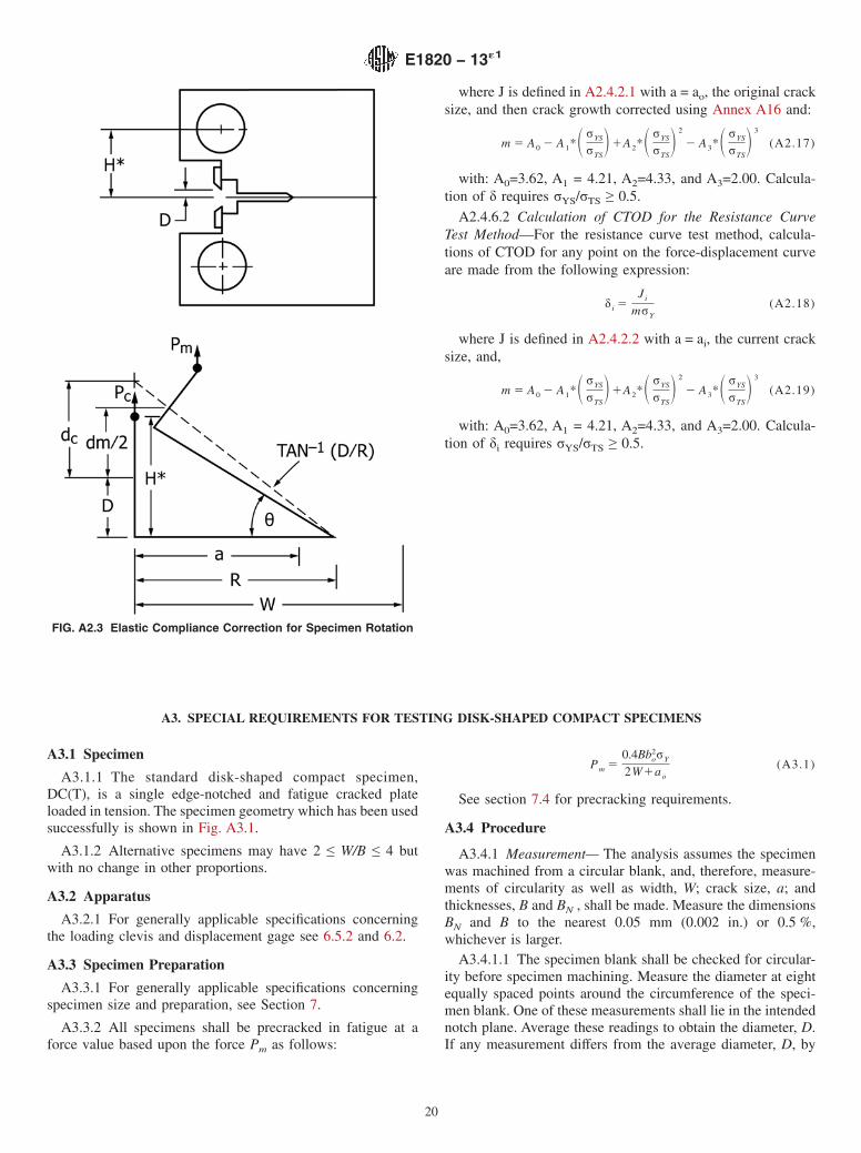
A3.1 Specimen

A3.1.1 The standard disk-shaped compact specimen,DC(T), is a single edge-notched and fatigue cracked plateloaded in tension. The specimen geometry which has been usedsuccessfully is shown in Fig. A3.1.

A3.1.2 Alternative specimens may have 2 ≤ W/B ≤ 4 butwith no change in other proportions.

A3.2 Apparatus

A3.2.1 For generally applicable specifications concerningthe loading clevis and displacement gage see 6.5.2 and 6.2.

A3.3 Specimen Preparation

A3.3.1 For generally applicable specifications concerningspecimen size and preparation, see Section 7.

A3.3.2 All specimens shall be precracked in fatigue at aforce value based upon the force Pm as follows:

Pm 50.4Bbo

2σY

2W1ao

(A3.1)

See section 7.4 for precracking requirements.

A3.4 Procedure

A3.4.1 Measurement— The analysis assumes the specimenwas machined from a circular blank, and, therefore, measure-ments of circularity as well as width, W; crack size, a; andthicknesses, B and BN , shall be made. Measure the dimensionsBN and B to the nearest 0.05 mm (0.002 in.) or 0.5 %,whichever is larger.

A3.4.1.1 The specimen blank shall be checked for circular-ity before specimen machining. Measure the diameter at eightequally spaced points around the circumference of the speci-men blank. One of these measurements shall lie in the intendednotch plane. Average these readings to obtain the diameter, D.If any measurement differs from the average diameter, D, by

FIG. A2.3 Elastic Compliance Correction for Specimen Rotation

E1820 − 13´1

20

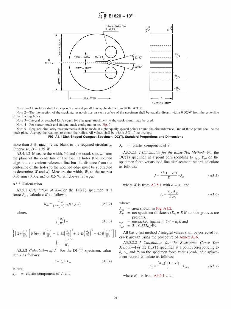
more than 5 %, machine the blank to the required circularity.Otherwise, D = 1.35 W.

A3.4.1.2 Measure the width, W, and the crack size, a, fromthe plane of the centerline of the loading holes (the notchededge is a convenient reference line but the distance from thecenterline of the holes to the notched edge must be subtractedto determine W and a). Measure the width, W, to the nearest0.05 mm (0.002 in.) or 0.5 %, whichever is larger.

A3.5 Calculation

A3.5.1 Calculation of K—For the DC(T) specimen at aforce P(i), calculate K as follows:

K~i!

5P

~i!

~BBNW!1/2 f~a i/W! (A3.2)

where:

fS ai

W D5 (A3.3)

H S 21ai

W D F 0.7614.8S ai

W D 2 11.58S ai

W D 2

111.43S ai

W D 3

2 4.08S ai

W D 4G JS 1 2

ai

W D 3/2

A3.5.2 Calculation of J—For the DC(T) specimen, calcu-late J as follows:

J 5 Jel1J pl (A3.4)

where:Jel = elastic component of J, and

Jpl = plastic component of J.

A3.5.2.1 J Calculation for the Basic Test Method—For theDC(T) specimen at a point corresponding to ν(i), P(i) on thespecimen force versus load-line displacement record, calculateas follows:

J 5K2~1 2 ν 2!

E1Jpl (A3.5)

where K is from A3.5.1 with a = ao, and

Jpl 5η pl A pl

BNbo

(A3.6)

where:Apl = area shown in Fig. A1.2,BN = net specimen thickness (BN = B if no side grooves are

present),bo = uncracked ligament, (W − ao), andηpl = 2 + 0.522bo/W.

All basic test method J integral values shall be corrected forcrack growth using the procedure of Annex A16.

A3.5.2.2 J Calculation for the Resistance Curve TestMethod—For the DC(T) specimen at a point corresponding toai, vi, and Pi on the specimen force versus load-line displace-ment record, calculate as follows:

J~i!

5~K

~i!!2 ~1 2 v2!

E1J pl~i!

(A3.7)

where K(i) is from A3.5.1 and:

NOTE 1—All surfaces shall be perpendicular and parallel as applicable within 0.002 W TIR.NOTE 2—The intersection of the crack starter notch tips on each surface of the specimen shall be equally distant within 0.005W from the centerline

of the loading holes.NOTE 3—Integral or attached knife edges for clip gage attachment to the crack mouth may be used.NOTE 4—For starter-notch and fatigue-crack configuration see Fig. 7.NOTE 5—Required circularity measurements shall be made at eight equally spaced points around the circumference. One of these points shall be the

notch plane. Average the readings to obtain the radius. All values shall be within 5 % of the average.FIG. A3.1 Disk-Shaped Compact Specimen, DC(T), Standard Proportions and Dimensions

E1820 − 13´1

21

J pl~i!5 (A3.8)

F Jpl~i21!1S η

~i21!

b~i21!

D Apl~i!2 Apl~i21!

BNG F 1 2 γ

~i21!

a~i!

2 a~i21!

b~i21!

Gwhere:η(i−1) = 2.0 + 0.522 b(i−1)/W, andγ(i−1) = 1.0 + 0.76 b(i−1)/W.

In the preceding equation, the quantity Apl(i) − Apl(i−1) is theincrement of plastic area under the force versus load-linedisplacement record between lines of constant displacement atpoints i−1 and i shown in Fig. A1.3. The quantity Jpl(i)

represents the total crack growth corrected plastic J at point iand is obtained in two steps by first incrementing the existingJpl(i−1) and then by modifying the total accumulated result toaccount for the crack growth increment. Accurate evaluation ofJpl(i) from the preceding relationship requires small and uni-form crack growth increments consistent with the suggestedelastic compliance spacing of Annex A8 and Annex A10. Thequantity Apl(i) can be calculated from the following equation:

Apl~i!5 A pl~i21!

1@P

~i!1P

~i21!# @νpl~i!2 νpl~i21!#

2(A3.9)

where:νpl(i) = plastic part of the load-line displacement,

νi − P(i)CLL(i), andCLL(i) = experimental compliance, (∆ν/∆P)i, corresponding

to the current crack size, ai.

For test methods that do not evaluate an experimental elasticcompliance, CLL(i) can be determined from the followingequation:

CLL~i!5

1EBe1 11

a~i!

W

1 2a

~i!

W2

2

3 (A3.10)

F 2.046219.6496S a~i!

W D 2 13.7346S a~i!

W D 2

16.1748S a~i!

W D 3Gwhere:Be = B − (B − BN)2/B.

The compliance estimated using Eq A3.10 should be verifiedby calibrating against the initial experimental compliance toassure the integrity of the load-line displacement measurementsystem.

In an elastic compliance test, the rotation correctedcompliance, Cc(i), described in A3.5.4 shall be used instead ofCLL(i) given above.

A3.5.3 Calculation of Crack Size—For a single-specimentest method using an elastic compliance technique on DC(T)specimens with crack opening displacements measured at theload-line, the crack size is given as follows:

a~i!

W5 0.998193 2 3.88087u10.187106u2120.3714u3(A3.11)

245.2125u 4144.5270u5

where:

u 51

@~BeECc~i!!1/211#

(A3.12)

where:Cc(i) = specimen crack opening compliance (∆v/∆P) on an

unloading/reloading sequence, corrected for rotation(see A3.5.4),

Be = B − (B − BN)2/B.

A3.5.4 To account for crack opening displacement in DC(T)specimens, the crack size estimation shall be corrected forrotation. Compliance shall be corrected as follows:

Cc~i!5

Ci

S H*R

sinθ i 2 cos θ iD S DR

sinθ i 2 cos θ iD (A3.13)

where (Fig. A2.3):

Ci = measured specimen elastic compliance (at the load-line),

H* = initial half-span of the load points (center of the pinholes),

R = radius of rotation of the crack centerline, (W + a)/2,where a is the updated crack size,

D = one half of the initial distance between the displace-ment measurement points,

θ = angle of rotation of a rigid body element about theunbroken midsection line, or

θ 5 sin21 F S dm

21DD

~D21R2!1/2G 2 tan21S D

R D , and (A3.14)

dm = total measured load-line displacement.

A3.5.5 Other compliance equations are acceptable if theresulting accuracy is equal to or greater than those describedand the accuracy has been verified experimentally.

A3.5.6 Calculation of CTOD:A3.5.6.1 Calculation of CTOD for the Basic Test Method—

For the basic test method calculations of CTOD for any pointon the force-displacement curve are made from the followingexpression:

δ 5J

mσY

(A3.15)

where J is defined in A3.5.2.1 with a = ao, the original cracksize and then crack growth corrected using Annex A16 and:

m 5 A0 2 A1*S σYS

σTSD1A2*S σYS

σTSD 2

2 A3*S σYS

σTSD 3

(A3.16)

with: A0=3.62, A1 = 4.21, A=4.33, and A3=2.00. Calculationof δ requires σYS/σTS ≥ 0.5.

A3.5.6.2 Calculation of CTOD for the Resistance CurveTest Method—For the resistance curve test method, calcula-tions of CTOD for any point on the force-displacement curveare made from the following expression:

δ 5Ji

mσY

(A3.17)

where J is defined in A3.5.2.2 with a = ai, the current cracksize and,

E1820 − 13´1

22

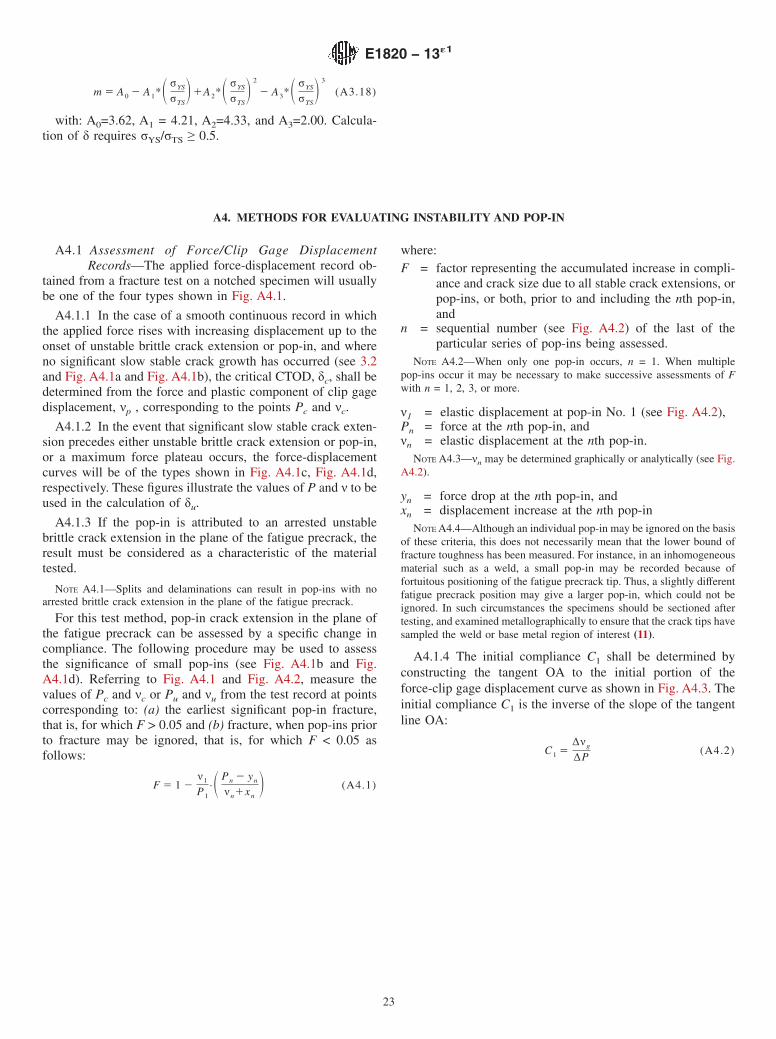
m 5 A0 2 A1*S σYS

σTSD1A2*S σYS

σTSD 2

2 A3*S σYS

σTSD 3

(A3.18)

with: A0=3.62, A1 = 4.21, A2=4.33, and A3=2.00. Calcula-tion of δ requires σYS/σTS ≥ 0.5.

A4. METHODS FOR EVALUATING INSTABILITY AND POP-IN

A4.1 Assessment of Force/Clip Gage DisplacementRecords—The applied force-displacement record ob-

tained from a fracture test on a notched specimen will usuallybe one of the four types shown in Fig. A4.1.

A4.1.1 In the case of a smooth continuous record in whichthe applied force rises with increasing displacement up to theonset of unstable brittle crack extension or pop-in, and whereno significant slow stable crack growth has occurred (see 3.2and Fig. A4.1a and Fig. A4.1b), the critical CTOD, δc, shall bedetermined from the force and plastic component of clip gagedisplacement, νp , corresponding to the points Pc and νc.

A4.1.2 In the event that significant slow stable crack exten-sion precedes either unstable brittle crack extension or pop-in,or a maximum force plateau occurs, the force-displacementcurves will be of the types shown in Fig. A4.1c, Fig. A4.1d,respectively. These figures illustrate the values of P and ν to beused in the calculation of δu.

A4.1.3 If the pop-in is attributed to an arrested unstablebrittle crack extension in the plane of the fatigue precrack, theresult must be considered as a characteristic of the materialtested.

NOTE A4.1—Splits and delaminations can result in pop-ins with noarrested brittle crack extension in the plane of the fatigue precrack.

For this test method, pop-in crack extension in the plane ofthe fatigue precrack can be assessed by a specific change incompliance. The following procedure may be used to assessthe significance of small pop-ins (see Fig. A4.1b and Fig.A4.1d). Referring to Fig. A4.1 and Fig. A4.2, measure thevalues of Pc and νc or Pu and νu from the test record at pointscorresponding to: (a) the earliest significant pop-in fracture,that is, for which F > 0.05 and (b) fracture, when pop-ins priorto fracture may be ignored, that is, for which F < 0.05 asfollows:

F 5 1 2ν1

P1

·S Pn 2 yn

νn1xnD (A4.1)

where:F = factor representing the accumulated increase in compli-

ance and crack size due to all stable crack extensions, orpop-ins, or both, prior to and including the nth pop-in,and

n = sequential number (see Fig. A4.2) of the last of theparticular series of pop-ins being assessed.

NOTE A4.2—When only one pop-in occurs, n = 1. When multiplepop-ins occur it may be necessary to make successive assessments of Fwith n = 1, 2, 3, or more.

ν1 = elastic displacement at pop-in No. 1 (see Fig. A4.2),Pn = force at the nth pop-in, andνn = elastic displacement at the nth pop-in.

NOTE A4.3—νn may be determined graphically or analytically (see Fig.A4.2).

yn = force drop at the nth pop-in, andxn = displacement increase at the nth pop-in

NOTE A4.4—Although an individual pop-in may be ignored on the basisof these criteria, this does not necessarily mean that the lower bound offracture toughness has been measured. For instance, in an inhomogeneousmaterial such as a weld, a small pop-in may be recorded because offortuitous positioning of the fatigue precrack tip. Thus, a slightly differentfatigue precrack position may give a larger pop-in, which could not beignored. In such circumstances the specimens should be sectioned aftertesting, and examined metallographically to ensure that the crack tips havesampled the weld or base metal region of interest (11).

A4.1.4 The initial compliance C1 shall be determined byconstructing the tangent OA to the initial portion of theforce-clip gage displacement curve as shown in Fig. A4.3. Theinitial compliance C1 is the inverse of the slope of the tangentline OA:

C1 5∆νg

∆P(A4.2)

E1820 − 13´1

23

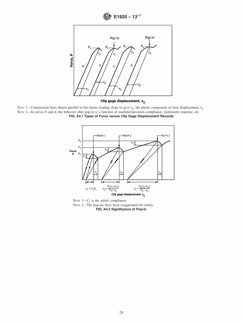
NOTE 1—Construction lines drawn parallel to the elastic loading slope to give νp, the plastic component of total displacement, νg.NOTE 2—In curves b and d, the behavior after pop-in is a function of machine/specimen compliance, instrument response, etc.

FIG. A4.1 Types of Force versus Clip Gage Displacement Records

NOTE 1—C1 is the initial compliance.NOTE 2—The pop-ins have been exaggerated for clarity.

FIG. A4.2 Significance of Pop-In

E1820 − 13´1

24

A5. METHOD FOR KIC DETERMINATION

A5.1 This annex has been removed from the standard. SeeTest Method E399.

A6. FRACTURE INSTABILITY TOUGHNESS DETERMINATION USING J

A6.1 This annex describes the method for characterizingfracture toughness values based on J, Jc, or Ju, for a fractureinstability and the associated requirements for qualifying thedata according to this test method. Data meeting all of thequalification requirements of 9.1 and those of this annex resultin qualified values of Jc or Ju. Data meeting the size require-ment result in a value of Jc that is insensitive to the in-planedimensions of the specimen.

A6.2 Fracture Instability Before Stable Tearing—Whenfracture occurs before stable tearing, a single-point toughnessvalue may be obtained labeled Jc.

A6.2.1 J is calculated at the final point of instability, usingthe J formulas for the basic method including the crack growthcorrection in Annex A16. This point is labeled JQc, a provi-sional Jc value.

A6.2.2 Qualification of JQc as Jc—JQc = Jc, a measure offracture toughness at instability without significant stable crackextension that is independent of in-plane dimensions, providedthe following two conditions are both met: (1) B, bo ≥ 100JQc/σY, and (2) crack extension ∆ap < 0.2 mm + JQc/2σY. Note

that even if these conditions are met, Jc may be dependent onthickness (length of crack front).

A6.3 Fracture Instability After Stable Tearing—Whenfracture occurs after stable tearing crack extension ∆ap > 0.2mm (0.008 in.) + JQc/2σY, a single-point fracture toughnessvalue may be obtained, labeled JQu. In addition, part of anR-curve may be developed or the final point may be used in theevaluation of an initiation toughness value JIc (these aredescribed in Annex A8 – Annex A11).

A6.3.1 J is calculated at the final point where instabilityoccurs using the J formulas for the basic method including thecrack growth correction of Annex A16. This point is a Ju value.

A6.3.2 Qualification of JQu as Ju—JQu = Ju if crack exten-sion ∆ap ≥ 0.2 mm (0.008 in.) + JQu/2σY.

A6.4 Significance of Jc and Ju—Values of JQc that meet thesize criteria are labeled Jc and are considered to be insensitiveto the in-plane dimensions of the specimen. For ferritic steelspecimens that have failed unstably by cleavage in the ductileto brittle transition, the analysis procedure of Test MethodE1921 is recommended. Values of JQc that do not meet validity

FIG. A4.3 Determination of Initial Compliance

E1820 − 13´1

25

remain JQc and may be size-dependent. Ju is not considered tobe a size-insensitive property and therefore is not subject to asize criterion. It is a characteristic of the material and specimengeometry and size. It signifies that at the test temperature thematerial is not completely ductile and can sustain only limitedR-curve behavior.

A7. FRACTURE INSTABILITY TOUGHNESS DETERMINATION USING CTOD (δ)

A7.1 This annex describes the method for characterizingfracture toughness values based on δ, δc, or δu for a fractureinstability and the associated requirements for qualifying thedata according to this test method. Data meeting all of thequalification requirements of 9.1 and those in this annex resultin qualified values of δc or δu. Data meeting the size require-ment result in a value of δc

* that is insensitive to in-planedimensions of the specimen.

A7.2 Fracture Instability Before Stable Tearing—Whenfracture occurs before stable tearing, a single-point toughnessvalue may be obtained labeled δc, the force Pc and the clip gagedisplacement υc, for δc are indicated in Fig. 1.

A7.2.1 δ is calculated at the final point, instability, using theδ formulas from Annex A1 – Annex A3. This point is labeledδQc, a provisional δc value.

A7.2.2 Qualification of δQc =δc*, a fracture toughness value

that is insensitive to the in-plane dimensions of the specimen,if the following two conditions are met: (1) B, bo ≥ 300 δQc,and (2) crack extension ∆ap < 0.2 mm (0.008 in.) + δQc/1.4.Data that fail to meet the size criterion based on B or bo, butstill meet the restriction on crack extension, are labeled δc.

A7.3 Fracture Instability After Stable Tearing—Whenfracture occurs after stable tearing, crack extension ∆ap ≥ 0.2mm (0.008 in.) + δQc/1.4, a single-point fracture toughnessvalue may be obtained, labeled δu. In addition, part of anR-curve may be developed or the final point may be used in theevaluation of an initiation toughness value (these are describedin Annex A8 – Annex A11).

A7.3.1 δ is calculated at the final point where instabilityoccurs, using the δ formulas for the basic method. This point islabeled δQu, a provisional δu value.

A7.3.2 Qualification of δQu as δu—δQu = δu, if crackextension, ∆ap > 0.2 mm (0.008 in.) + δQu/1.4.

A7.3.3 Significance of δc and δu—Values of δQc that meetthe qualification requirements are labeled δc

* and are consid-ered to be insensitive to the in-plane dimensions of thespecimen. Values of δQc that do not meet the size requirementare labeled δc and may be size-dependent. δu is not consideredto be a size-insensitive property and, therefore, is not subject toa size criterion. It is a characteristic of the material andspecimen geometry and size. It signifies that at the testtemperature the material is not completely ductile and cansustain only limited R-curve behavior.

A8. J-R CURVE DETERMINATION

NOTE A8.1—Annex A8 – Annex A11 cover methods for evaluatingtoughness for stable tearing.

A8.1 This method describes a single-specimen techniquefor determining the J-R curve of metallic materials. The J-Rcurve consists of a plot of J versus crack extension in theregion of J controlled growth. The J-R curve is qualifiedprovided that the criteria of 9.1 and A8.3 are satisfied.

A8.2 J Calculation:

A8.2.1 J can be calculated at any point on the force versusload-line displacement record using the equations suggested inthe calculation section of Annex A1 – Annex A3 for thedifferent specimen geometries.

A8.2.2 If the basic method is used, J values must be crackgrowth corrected using the procedure of Annex A16. In thiscase, crack size values are obtained from direct optical mea-surements from the specimen fracture surfaces using theprocedure of 8.5.

A8.2.3 If a resistance curve method is used, the values ofcrack size are calculated using the compliance equationsdescribed in Annex A1 – Annex A3 (or an alternative methodfor measuring crack size). The rotation correction shall beapplied to account for geometry changes due to deformationfor the compact, C(T), and disk-shaped compact, DC(T),specimens.

E1820 − 13´1

26

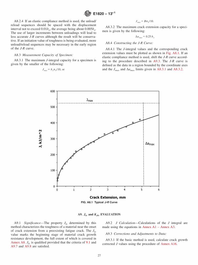
A8.2.4 If an elastic compliance method is used, the unload/reload sequences should be spaced with the displacementinterval not to exceed 0.01bo, the average being about 0.005bo.The use of larger increments between unloadings will lead toless accurate J-R curves although the result will be conserva-tive. If an initiation value of toughness is being evaluated, moreunload/reload sequences may be necessary in the early regionof the J-R curve.

A8.3 Measurement Capacity of Specimen:

A8.3.1 The maximum J-integral capacity for a specimen isgiven by the smaller of the following:

Jmax 5 boσY/10, or

Jmax 5 BσY/10.

A8.3.2 The maximum crack extension capacity for a speci-men is given by the following:

∆amax 5 0.25 bo

A8.4 Constructing the J-R Curve:

A8.4.1 The J-integral values and the corresponding crackextension values must be plotted as shown in Fig. A8.1. If anelastic compliance method is used, shift the J-R curve accord-ing to the procedure described in A9.3. The J-R curve isdefined as the data in a region bounded by the coordinate axesand the Jmax and ∆amax limits given in A8.3.1 and A8.3.2.

A9. JIc and KJIc EVALUATION

A9.1 Significance—The property JIc determined by thismethod characterizes the toughness of a material near the onsetof crack extension from a preexisting fatigue crack. The JIc

value marks the beginning stage of material crack growthresistance development, the full extent of which is covered inAnnex A8. JIc is qualified provided that the criteria of 9.1 andA9.7 and A9.8 are satisfied.

A9.2 J Calculation—Calculations of the J integral aremade using the equations in Annex A1 – Annex A3.

A9.3 Corrections and Adjustments to Data:

A9.3.1 If the basic method is used, calculate crack growthcorrected J values using the procedure of Annex A16.

FIG. A8.1 Typical J-R Curve

E1820 − 13´1

27

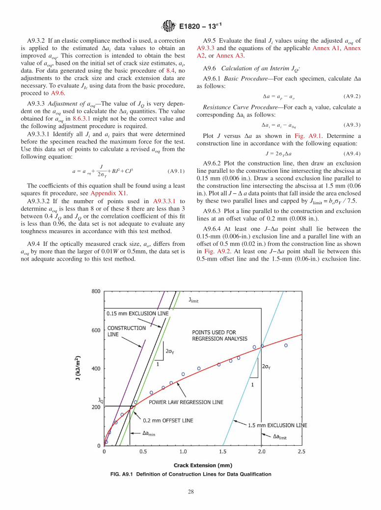
A9.3.2 If an elastic compliance method is used, a correctionis applied to the estimated ∆ai data values to obtain animproved aoq. This correction is intended to obtain the bestvalue of aoq, based on the initial set of crack size estimates, ai,data. For data generated using the basic procedure of 8.4, noadjustments to the crack size and crack extension data arenecessary. To evaluate JIc using data from the basic procedure,proceed to A9.6.

A9.3.3 Adjustment of aoq—The value of JQ is very depen-dent on the aoq used to calculate the ∆ai quantities. The valueobtained for aoq in 8.6.3.1 might not be the correct value andthe following adjustment procedure is required.

A9.3.3.1 Identify all Ji and ai pairs that were determinedbefore the specimen reached the maximum force for the test.Use this data set of points to calculate a revised aoq from thefollowing equation:

a 5 a oq1J

2σY

1BJ21CJ3 (A9.1)

The coefficients of this equation shall be found using a leastsquares fit procedure, see Appendix X1.

A9.3.3.2 If the number of points used in A9.3.3.1 todetermine aoq is less than 8 or of these 8 there are less than 3between 0.4 JQ and JQ or the correlation coefficient of this fitis less than 0.96, the data set is not adequate to evaluate anytoughness measures in accordance with this test method.

A9.4 If the optically measured crack size, ao, differs fromaoq by more than the larger of 0.01W or 0.5mm, the data set isnot adequate according to this test method.

A9.5 Evaluate the final Ji values using the adjusted aoq ofA9.3.3 and the equations of the applicable Annex A1, AnnexA2, or Annex A3.

A9.6 Calculation of an Interim JQ:

A9.6.1 Basic Procedure—For each specimen, calculate ∆aas follows:

∆a 5 ap 2 ao (A9.2)

Resistance Curve Procedure—For each ai value, calculate acorresponding ∆ai as follows:

∆ai 5 ai 2 a0q (A9.3)

Plot J versus ∆a as shown in Fig. A9.1. Determine aconstruction line in accordance with the following equation:

J 5 2σY∆a (A9.4)

A9.6.2 Plot the construction line, then draw an exclusionline parallel to the construction line intersecting the abscissa at0.15 mm (0.006 in.). Draw a second exclusion line parallel tothe construction line intersecting the abscissa at 1.5 mm (0.06in.). Plot all J − ∆ a data points that fall inside the area enclosedby these two parallel lines and capped by Jlimit = boσY ⁄ 7.5.

A9.6.3 Plot a line parallel to the construction and exclusionlines at an offset value of 0.2 mm (0.008 in.).

A9.6.4 At least one J–∆a point shall lie between the0.15-mm (0.006-in.) exclusion line and a parallel line with anoffset of 0.5 mm (0.02 in.) from the construction line as shownin Fig. A9.2. At least one J−∆a point shall lie between this0.5-mm offset line and the 1.5-mm (0.06-in.) exclusion line.

FIG. A9.1 Definition of Construction Lines for Data Qualification

E1820 − 13´1

28

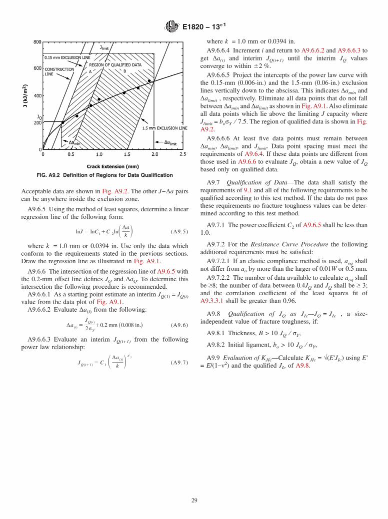
Acceptable data are shown in Fig. A9.2. The other J−∆a pairscan be anywhere inside the exclusion zone.

A9.6.5 Using the method of least squares, determine a linearregression line of the following form:

lnJ 5 lnC11C 2lnS ∆ak D (A9.5)

where k = 1.0 mm or 0.0394 in. Use only the data whichconform to the requirements stated in the previous sections.Draw the regression line as illustrated in Fig. A9.1.

A9.6.6 The intersection of the regression line of A9.6.5 withthe 0.2-mm offset line defines JQ and ∆aQ. To determine thisintersection the following procedure is recommended.

A9.6.6.1 As a starting point estimate an interim JQ(1) = JQ(i)

value from the data plot of Fig. A9.1.A9.6.6.2 Evaluate ∆a(i) from the following:

∆a~i!

5JQ~i!

2σY

10.2 mm ~0.008 in.! (A9.6)

A9.6.6.3 Evaluate an interim JQ(i+1) from the followingpower law relationship:

JQ~i11!5 C1 S ∆a

~i!

k D C2

(A9.7)

where k = 1.0 mm or 0.0394 in.A9.6.6.4 Increment i and return to A9.6.6.2 and A9.6.6.3 to

get ∆a(i) and interim JQ(i+1) until the interim JQ valuesconverge to within 62 %.

A9.6.6.5 Project the intercepts of the power law curve withthe 0.15-mm (0.006-in.) and the 1.5-mm (0.06-in.) exclusionlines vertically down to the abscissa. This indicates ∆amin and∆alimit , respectively. Eliminate all data points that do not fallbetween ∆amin and ∆alimit as shown in Fig. A9.1. Also eliminateall data points which lie above the limiting J capacity whereJlimit = boσY ⁄ 7.5. The region of qualified data is shown in Fig.A9.2.

A9.6.6.6 At least five data points must remain between∆amin, ∆alimit, and Jlimit. Data point spacing must meet therequirements of A9.6.4. If these data points are different fromthose used in A9.6.6 to evaluate JQ, obtain a new value of JQ

based only on qualified data.

A9.7 Qualification of Data—The data shall satisfy therequirements of 9.1 and all of the following requirements to bequalified according to this test method. If the data do not passthese requirements no fracture toughness values can be deter-mined according to this test method.

A9.7.1 The power coefficient C2 of A9.6.5 shall be less than1.0.

A9.7.2 For the Resistance Curve Procedure the followingadditional requirements must be satisfied:

A9.7.2.1 If an elastic compliance method is used, aoq shallnot differ from ao by more than the larger of 0.01W or 0.5 mm.

A9.7.2.2 The number of data available to calculate aoq shallbe ≥8; the number of data between 0.4JQ and JQ shall be ≥ 3;and the correlation coefficient of the least squares fit ofA9.3.3.1 shall be greater than 0.96.

A9.8 Qualification of JQ as JIc—JQ = JIc , a size-independent value of fracture toughness, if:

A9.8.1 Thickness, B > 10 JQ ⁄ σY,

A9.8.2 Initial ligament, bo > 10 JQ ⁄ σY,

A9.9 Evaluation of KJIc—Calculate KJIc = √(E'JIc) using E'= E/(1−ν2) and the qualified JIc of A9.8.

FIG. A9.2 Definition of Regions for Data Qualification

E1820 − 13´1

29

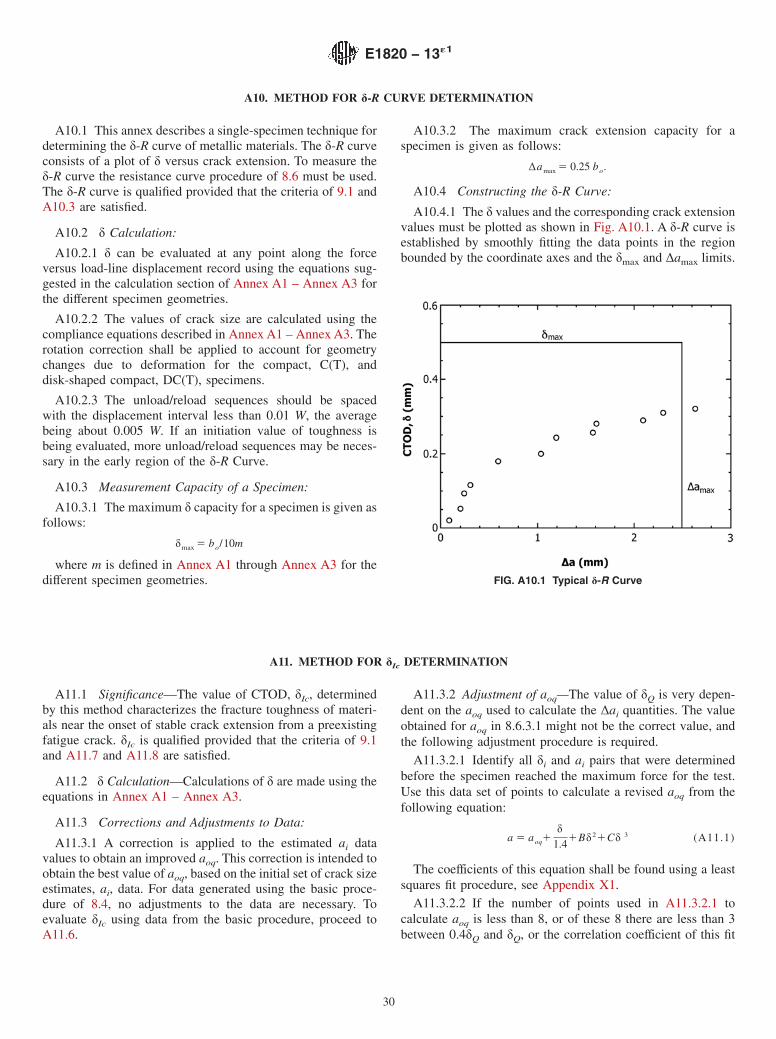
A10. METHOD FOR δ-R CURVE DETERMINATION

A10.1 This annex describes a single-specimen technique fordetermining the δ-R curve of metallic materials. The δ-R curveconsists of a plot of δ versus crack extension. To measure theδ-R curve the resistance curve procedure of 8.6 must be used.The δ-R curve is qualified provided that the criteria of 9.1 andA10.3 are satisfied.

A10.2 δ Calculation:

A10.2.1 δ can be evaluated at any point along the forceversus load-line displacement record using the equations sug-gested in the calculation section of Annex A1 – Annex A3 forthe different specimen geometries.

A10.2.2 The values of crack size are calculated using thecompliance equations described in Annex A1 – Annex A3. Therotation correction shall be applied to account for geometrychanges due to deformation for the compact, C(T), anddisk-shaped compact, DC(T), specimens.

A10.2.3 The unload/reload sequences should be spacedwith the displacement interval less than 0.01 W, the averagebeing about 0.005 W. If an initiation value of toughness isbeing evaluated, more unload/reload sequences may be neces-sary in the early region of the δ-R Curve.

A10.3 Measurement Capacity of a Specimen:

A10.3.1 The maximum δ capacity for a specimen is given asfollows:

δmax 5 bo/10m

where m is defined in Annex A1 through Annex A3 for thedifferent specimen geometries.

A10.3.2 The maximum crack extension capacity for aspecimen is given as follows:

∆amax 5 0.25 bo.

A10.4 Constructing the δ-R Curve:

A10.4.1 The δ values and the corresponding crack extensionvalues must be plotted as shown in Fig. A10.1. A δ-R curve isestablished by smoothly fitting the data points in the regionbounded by the coordinate axes and the δmax and ∆amax limits.

A11. METHOD FOR δIc DETERMINATION

A11.1 Significance—The value of CTOD, δIc, determinedby this method characterizes the fracture toughness of materi-als near the onset of stable crack extension from a preexistingfatigue crack. δIc is qualified provided that the criteria of 9.1and A11.7 and A11.8 are satisfied.

A11.2 δ Calculation—Calculations of δ are made using theequations in Annex A1 – Annex A3.

A11.3 Corrections and Adjustments to Data:

A11.3.1 A correction is applied to the estimated ai datavalues to obtain an improved aoq. This correction is intended toobtain the best value of aoq, based on the initial set of crack sizeestimates, ai, data. For data generated using the basic proce-dure of 8.4, no adjustments to the data are necessary. Toevaluate δIc using data from the basic procedure, proceed toA11.6.

A11.3.2 Adjustment of aoq—The value of δQ is very depen-dent on the aoq used to calculate the ∆ai quantities. The valueobtained for aoq in 8.6.3.1 might not be the correct value, andthe following adjustment procedure is required.

A11.3.2.1 Identify all δi and ai pairs that were determinedbefore the specimen reached the maximum force for the test.Use this data set of points to calculate a revised aoq from thefollowing equation:

a 5 aoq1δ

1.41Bδ21Cδ 3 (A11.1)

The coefficients of this equation shall be found using a leastsquares fit procedure, see Appendix X1.

A11.3.2.2 If the number of points used in A11.3.2.1 tocalculate aoq is less than 8, or of these 8 there are less than 3between 0.4δQ and δQ, or the correlation coefficient of this fit

FIG. A10.1 Typical δ-R Curve

E1820 − 13´1

30

is < 0.96, the data set is not adequate to evaluate any toughnessmeasures in accordance with this method.

A11.4 If the optically measured crack size, ao, differs fromaoq by more than the larger of 0.01 W or 0.5 mm, the data setis not adequate in accordance with this method.

A11.5 Evaluate the final δi values using the adjusted aoq ofA11.3.2.1 and the equations of the applicable Annex A1,Annex A2, or Annex A3.

A11.6 Calculation of an Interim δQ:

A11.6.1 Basic Procedure—for each specimen, calculate ∆aas follows:

∆a 5 ap 2 ao (A11.2)

Resistance Curve Procedure—for each ai value, calculate acorresponding ∆ai as follows:

∆ai 5 ai 2 a0q (A11.3)

Plot δ versus ∆a as shown in Fig. A11.1. Draw a constructionline in accordance with the following equation:

δ 5 1.4 ∆a (A11.4)

A11.6.2 Plot the construction line. Draw an exclusion lineparallel to the construction line intersecting the abscissa at 0.15mm (0.006 in.) as shown in Fig. A11.1. Draw a secondexclusion line intersecting the abscissa at 1.5 mm (0.06 in.).Plot all δ-∆ap data points that fall inside the area enclosed bythese two parallel lines and capped by δlimit = bo ⁄ 7.5m, wherem is defined in Annex A1 through Annex A3 for the differentspecimen geometries.

A11.6.3 One δ-∆ap point must lie between the 0.15-mm(0.006-in.) exclusion line and a parallel line with an offset of

0.5 mm (0.02 in.) from the construction line. One δ-∆ap pointmust lie between a line parallel to the construction line at anoffset of 0.5 mm (0.020 in.) and the 1.5-mm exclusion line.Acceptable data is shown in Fig. A11.2 with one point in ZoneA and one point in Zone B. The other δ-∆ap pairs can be placedanywhere inside the exclusion zone.

A11.6.4 Plot a line parallel to the construction line andexclusion lines at an offset value of 0.2 mm (0.008 in.).

A11.6.5 To establish a crack initiation measurement pointunder dominant slow-stable crack growth, a power law curvefitting procedure shall be used. This has the following form:

δQ 5 C1 S ∆ak D C2

(A11.5)

where k = 1 mm (or 0.0394 in.) depending upon units used.This power law can be determined by using a method of leastsquares to determine a linear regression line of the followingform:

lnδ 5 lnC11C 2lnS ∆ak D (A11.6)

Use only the data that conform to the criteria stated in theprevious sections. Plot the regression line as illustrated in Fig.A11.1.

A11.6.6 The intersection of the regression line of A11.6.4with the offset line of A11.6.5 defines δQ and ∆aQ. Todetermine this intersection the following procedure is recom-mended:

A11.6.6.1 Estimate a δQ(1) value from the data plot of Fig.A11.1.

A11.6.6.2 Evaluate ∆ap(1) from the following:

FIG. A11.1 Definition of Construction Lines for Data Qualification

E1820 − 13´1

31

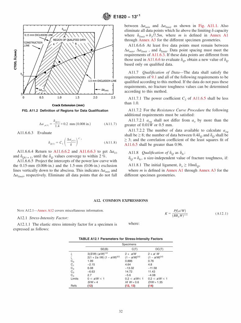
∆a p~1!5

δQ~1!

1.410.2 mm ~0.008 in.! (A11.7)

A11.6.6.3 Evaluate

δQ~1!5 C1 S ∆ap~1!

k D C 2

(A11.8)

A11.6.6.4 Return to A11.6.6.2 and A11.6.6.3 to get ∆a(i)

and δQ(i + 1) until the δQ values converge to within 2 %.A11.6.6.5 Project the intercepts of the power law curve with

the 0.15-mm (0.006-in.) and the 1.5-mm (0.06-in.) exclusionlines vertically down to the abscissa. This indicates ∆amin and∆alimit, respectively. Eliminate all data points that do not fall

between ∆amin and ∆alimit as shown in Fig. A11.1. Alsoeliminate all data points which lie above the limiting δ capacitywhere δlimit = bo/7.5m, where m is defined in Annex A1through Annex A3 for the different specimen geometries.

A11.6.6.6 At least five data points must remain between∆amin, ∆alimit , and δlimit. Data point spacing must meet therequirements of A11.6.3. If these data points are different fromthose used in A11.6.6 to evaluate δQ, obtain a new value of δQ

based only on qualified data.

A11.7 Qualification of Data—The data shall satisfy therequirements of 9.1 and all of the following requirements to bequalified according to this method. If the data do not pass theserequirements, no fracture toughness values can be determinedaccording to this method.

A11.7.1 The power coefficient C2 of A11.6.5 shall be lessthan 1.0.

A11.7.2 For the Resistance Curve Procedure the followingadditional requirements must be satisfied:

A11.7.2.1 aoq shall not differ from ao by more than thegreater of 0.01W or 0.5 mm.

A11.7.2.2 The number of data available to calculate aoq

shall be ≥ 8; the number of data between 0.4δQ and δQ shall be≥ 3; and the correlation coefficient of the least squares fit ofA11.6.5 shall be greater than 0.96.

A11.8 Qualification of δQ as δIc:δQ = δIc, a size-independent value of fracture toughness, if:

A11.8.1 The initial ligament, bo ≥ 10mδQ,where m is defined in Annex A1 through Annex A3 for the

different specimen geometries.

A12. COMMON EXPRESSIONS

NOTE A12.1—Annex A12 covers miscellaneous information.

A12.1 Stress-Intensity Factor:

A12.1.1 The elastic stress intensity factor for a specimen isexpressed as follows:

K 5Pf~a/W!

~BBNW!1/2 (A12.1)

where:

FIG. A11.2 Definition of Regions for Data Qualification

TABLE A12.1 Parameters for Stress-Intensity Factors

Specimens

SE(B) C(T) DC(T)

ξ 3(S/W) (a/W)1/2 2 + a/W 2 + a/ Wζ 2(1 + 2a /W) (1 − a/W)3/2 (1 − a/W)3/2 (1 − a/W)3/2

C0 1.99 0.886 0.76C1 −2.15 4.64 4.8C2 6.08 −13.32 −11.58C3 −6.63 14.72 11.43C4 2.7 −5.6 −4.08Limits 0 # a/W # 1 0.2 # a/W# 1 0.2 # a/W # 1

S/W = 4 H/ W = 0.6 D/W = 1.35Refs (12) (12, 13) (14)

E1820 − 13´1

32

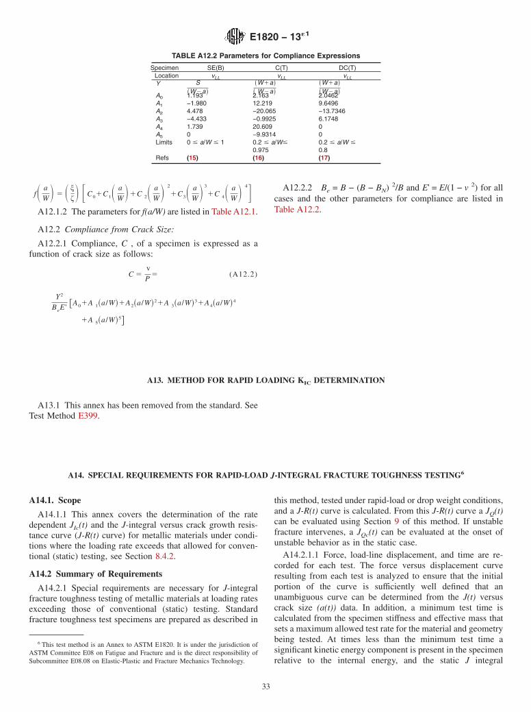
fS aW D 5 S ξ

ζ D FC01C1S aW D1C 2S a

W D 2

1C3S aW D 3

1C 4S aW D 4G

A12.1.2 The parameters for f(a/W) are listed in Table A12.1.

A12.2 Compliance from Crack Size:

A12.2.1 Compliance, C , of a specimen is expressed as afunction of crack size as follows:

C 5vP

5 (A12.2)

Y2

BeE ' @A01A 1~a/W!1A2~a/W!21A 3~a/W!31A4~a/W!4

1A 5~a/W!5#

A12.2.2 Be = B − (B − BN) 2/B and E' = E/(1 − v 2) for allcases and the other parameters for compliance are listed inTable A12.2.

A13. METHOD FOR RAPID LOADING KIC DETERMINATION

A13.1 This annex has been removed from the standard. SeeTest Method E399.

A14. SPECIAL REQUIREMENTS FOR RAPID-LOAD J-INTEGRAL FRACTURE TOUGHNESS TESTING6

A14.1. Scope

A14.1.1 This annex covers the determination of the ratedependent JIc(t) and the J-integral versus crack growth resis-tance curve (J-R(t) curve) for metallic materials under condi-tions where the loading rate exceeds that allowed for conven-tional (static) testing, see Section 8.4.2.

A14.2 Summary of Requirements

A14.2.1 Special requirements are necessary for J-integralfracture toughness testing of metallic materials at loading ratesexceeding those of conventional (static) testing. Standardfracture toughness test specimens are prepared as described in

this method, tested under rapid-load or drop weight conditions,and a J-R(t) curve is calculated. From this J-R(t) curve a JQ(t)can be evaluated using Section 9 of this method. If unstablefracture intervenes, a JQc(t) can be evaluated at the onset ofunstable behavior as in the static case.

A14.2.1.1 Force, load-line displacement, and time are re-corded for each test. The force versus displacement curveresulting from each test is analyzed to ensure that the initialportion of the curve is sufficiently well defined that anunambiguous curve can be determined from the J(t) versuscrack size (a(t)) data. In addition, a minimum test time iscalculated from the specimen stiffness and effective mass thatsets a maximum allowed test rate for the material and geometrybeing tested. At times less than the minimum test time asignificant kinetic energy component is present in the specimenrelative to the internal energy, and the static J integral

6 This test method is an Annex to ASTM E1820. It is under the jurisdiction ofASTM Committee E08 on Fatigue and Fracture and is the direct responsibility ofSubcommittee E08.08 on Elastic-Plastic and Fracture Mechanics Technology.

TABLE A12.2 Parameters for Compliance Expressions

Specimen SE(B) C(T) DC(T)Location vLL vLL vLL

Y SsW2ad

sW1ads W2ad

sW1adsW2adA0 1.193 2.163 2.0462

A1 −1.980 12.219 9.6496A2 4.478 −20.065 −13.7346A3 −4.433 −0.9925 6.1748A4 1.739 20.609 0A5 0 −9.9314 0Limits 0 # a/W # 1 0.2 # a/W# 0.2 # a/W #

0.975 0.8Refs (15) (16) (17)

E1820 − 13´1

33

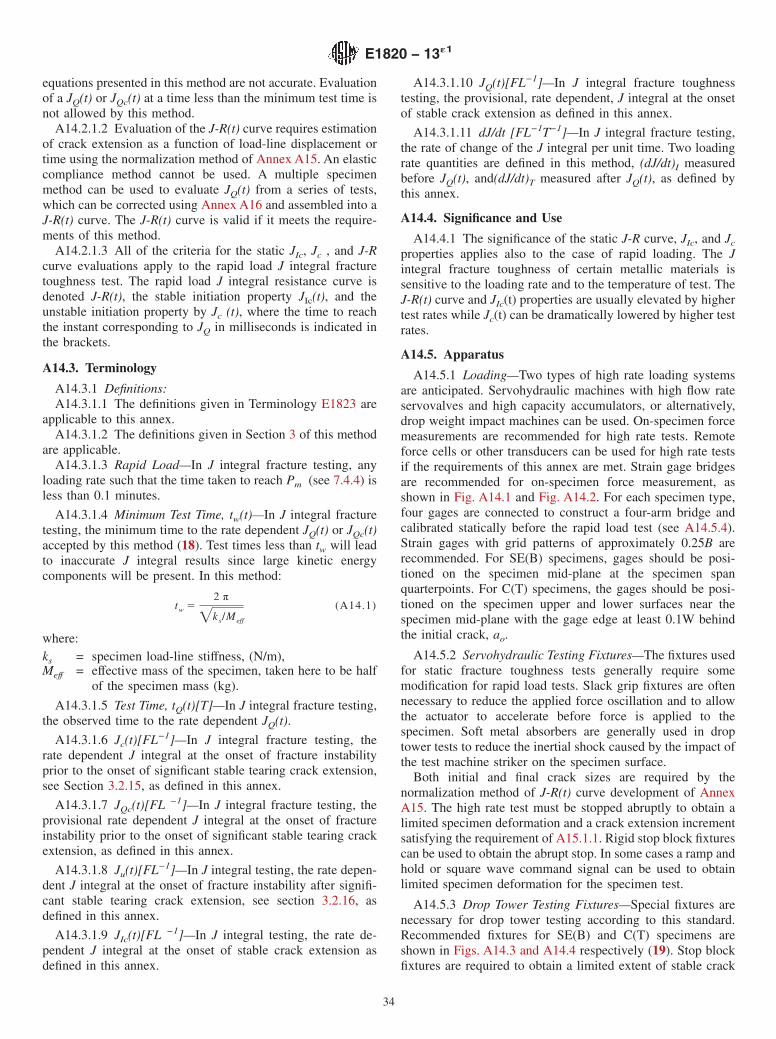
equations presented in this method are not accurate. Evaluationof a JQ(t) or JQc(t) at a time less than the minimum test time isnot allowed by this method.

A14.2.1.2 Evaluation of the J-R(t) curve requires estimationof crack extension as a function of load-line displacement ortime using the normalization method of Annex A15. An elasticcompliance method cannot be used. A multiple specimenmethod can be used to evaluate JQ(t) from a series of tests,which can be corrected using Annex A16 and assembled into aJ-R(t) curve. The J-R(t) curve is valid if it meets the require-ments of this method.

A14.2.1.3 All of the criteria for the static JIc, Jc , and J-Rcurve evaluations apply to the rapid load J integral fracturetoughness test. The rapid load J integral resistance curve isdenoted J-R(t), the stable initiation property JIc(t), and theunstable initiation property by Jc (t), where the time to reachthe instant corresponding to JQ in milliseconds is indicated inthe brackets.

A14.3. Terminology

A14.3.1 Definitions:A14.3.1.1 The definitions given in Terminology E1823 are

applicable to this annex.A14.3.1.2 The definitions given in Section 3 of this method

are applicable.A14.3.1.3 Rapid Load—In J integral fracture testing, any

loading rate such that the time taken to reach Pm (see 7.4.4) isless than 0.1 minutes.

A14.3.1.4 Minimum Test Time, tw(t)—In J integral fracturetesting, the minimum time to the rate dependent JQ(t) or JQc(t)accepted by this method (18). Test times less than tw will leadto inaccurate J integral results since large kinetic energycomponents will be present. In this method:

tw 52 π

=ks/Meff

(A14.1)

where:ks = specimen load-line stiffness, (N/m),Meff = effective mass of the specimen, taken here to be half

of the specimen mass (kg).

A14.3.1.5 Test Time, tQ(t)[T]—In J integral fracture testing,the observed time to the rate dependent JQ(t).

A14.3.1.6 Jc(t)[FL−1]—In J integral fracture testing, therate dependent J integral at the onset of fracture instabilityprior to the onset of significant stable tearing crack extension,see Section 3.2.15, as defined in this annex.

A14.3.1.7 JQc(t)[FL −1]—In J integral fracture testing, theprovisional rate dependent J integral at the onset of fractureinstability prior to the onset of significant stable tearing crackextension, as defined in this annex.

A14.3.1.8 Ju(t)[FL−1]—In J integral testing, the rate depen-dent J integral at the onset of fracture instability after signifi-cant stable tearing crack extension, see section 3.2.16, asdefined in this annex.

A14.3.1.9 JIc(t)[FL −1]—In J integral testing, the rate de-pendent J integral at the onset of stable crack extension asdefined in this annex.

A14.3.1.10 JQ(t)[FL−1]—In J integral fracture toughnesstesting, the provisional, rate dependent, J integral at the onsetof stable crack extension as defined in this annex.

A14.3.1.11 dJ/dt [FL−1T−1]—In J integral fracture testing,the rate of change of the J integral per unit time. Two loadingrate quantities are defined in this method, (dJ/dt)I measuredbefore JQ(t), and(dJ/dt)T measured after JQ(t), as defined bythis annex.

A14.4. Significance and Use

A14.4.1 The significance of the static J-R curve, JIc, and Jc

properties applies also to the case of rapid loading. The Jintegral fracture toughness of certain metallic materials issensitive to the loading rate and to the temperature of test. TheJ-R(t) curve and JIc(t) properties are usually elevated by highertest rates while Jc(t) can be dramatically lowered by higher testrates.

A14.5. Apparatus

A14.5.1 Loading—Two types of high rate loading systemsare anticipated. Servohydraulic machines with high flow rateservovalves and high capacity accumulators, or alternatively,drop weight impact machines can be used. On-specimen forcemeasurements are recommended for high rate tests. Remoteforce cells or other transducers can be used for high rate testsif the requirements of this annex are met. Strain gage bridgesare recommended for on-specimen force measurement, asshown in Fig. A14.1 and Fig. A14.2. For each specimen type,four gages are connected to construct a four-arm bridge andcalibrated statically before the rapid load test (see A14.5.4).Strain gages with grid patterns of approximately 0.25B arerecommended. For SE(B) specimens, gages should be posi-tioned on the specimen mid-plane at the specimen spanquarterpoints. For C(T) specimens, the gages should be posi-tioned on the specimen upper and lower surfaces near thespecimen mid-plane with the gage edge at least 0.1W behindthe initial crack, ao.

A14.5.2 Servohydraulic Testing Fixtures—The fixtures usedfor static fracture toughness tests generally require somemodification for rapid load tests. Slack grip fixtures are oftennecessary to reduce the applied force oscillation and to allowthe actuator to accelerate before force is applied to thespecimen. Soft metal absorbers are generally used in droptower tests to reduce the inertial shock caused by the impact ofthe test machine striker on the specimen surface.

Both initial and final crack sizes are required by thenormalization method of J-R(t) curve development of AnnexA15. The high rate test must be stopped abruptly to obtain alimited specimen deformation and a crack extension incrementsatisfying the requirement of A15.1.1. Rigid stop block fixturescan be used to obtain the abrupt stop. In some cases a ramp andhold or square wave command signal can be used to obtainlimited specimen deformation for the specimen test.

A14.5.3 Drop Tower Testing Fixtures—Special fixtures arenecessary for drop tower testing according to this standard.Recommended fixtures for SE(B) and C(T) specimens areshown in Figs. A14.3 and A14.4 respectively (19). Stop blockfixtures are required to obtain a limited extent of stable crack

E1820 − 13´1

34

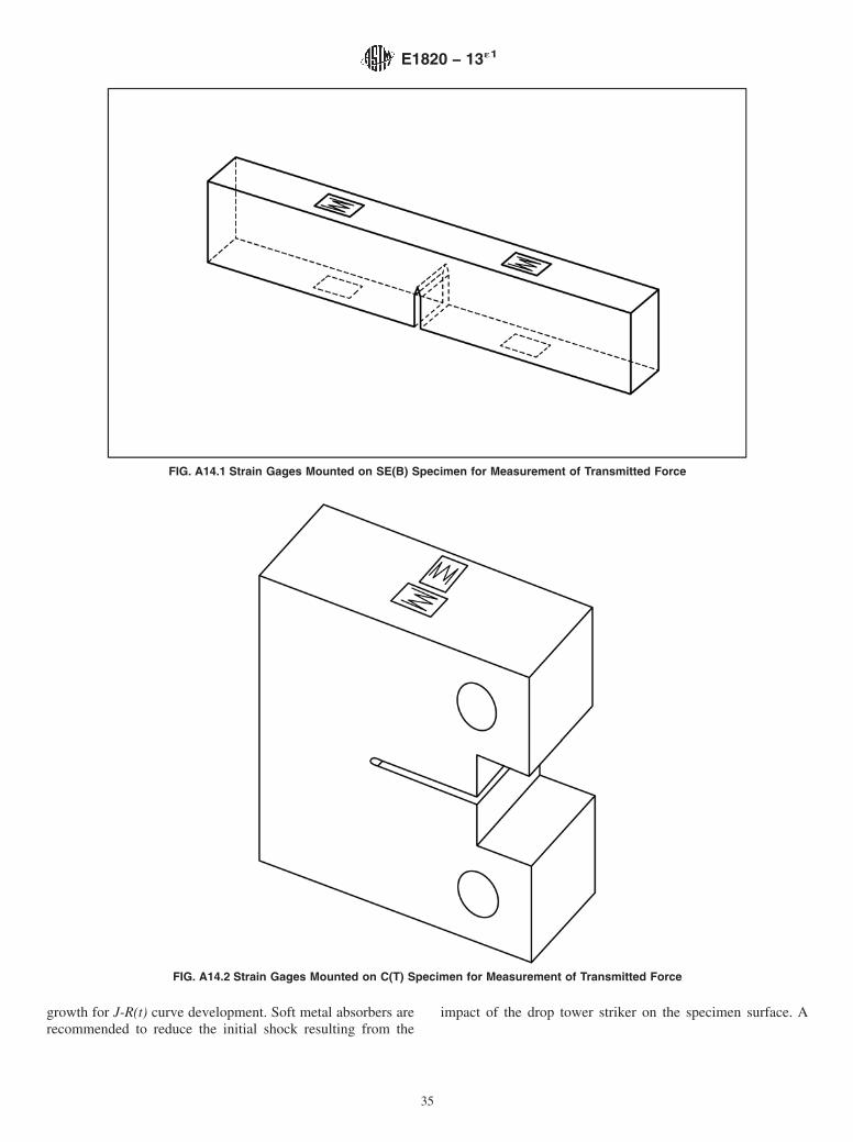
growth for J-R(t) curve development. Soft metal absorbers arerecommended to reduce the initial shock resulting from the

impact of the drop tower striker on the specimen surface. A

FIG. A14.1 Strain Gages Mounted on SE(B) Specimen for Measurement of Transmitted Force

FIG. A14.2 Strain Gages Mounted on C(T) Specimen for Measurement of Transmitted Force

E1820 − 13´1

35

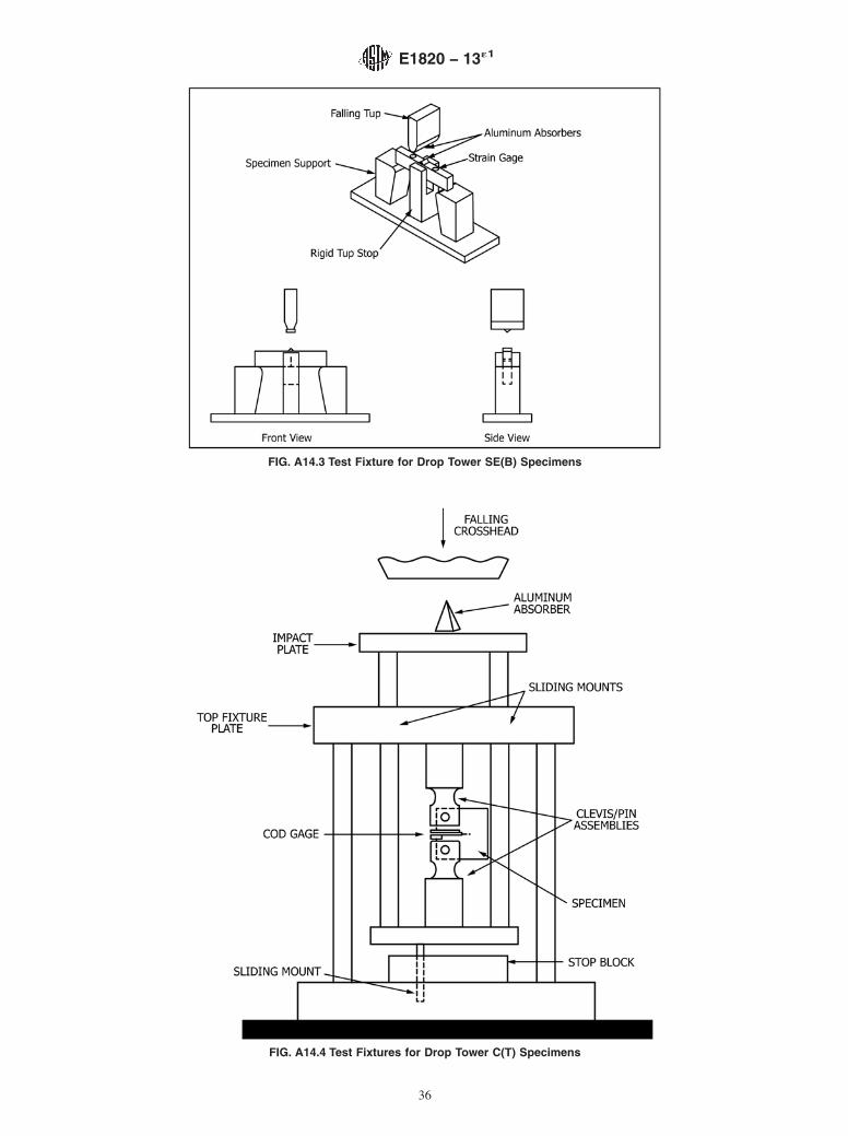
FIG. A14.3 Test Fixture for Drop Tower SE(B) Specimens

FIG. A14.4 Test Fixtures for Drop Tower C(T) Specimens

E1820 − 13´1

36

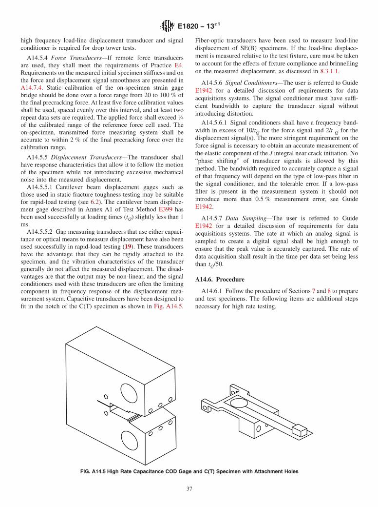
high frequency load-line displacement transducer and signalconditioner is required for drop tower tests.

A14.5.4 Force Transducers—If remote force transducersare used, they shall meet the requirements of Practice E4.Requirements on the measured initial specimen stiffness and onthe force and displacement signal smoothness are presented inA14.7.4. Static calibration of the on-specimen strain gagebridge should be done over a force range from 20 to 100 % ofthe final precracking force. At least five force calibration valuesshall be used, spaced evenly over this interval, and at least tworepeat data sets are required. The applied force shall exceed 1⁄4of the calibrated range of the reference force cell used. Theon-specimen, transmitted force measuring system shall beaccurate to within 2 % of the final precracking force over thecalibration range.

A14.5.5 Displacement Transducers—The transducer shallhave response characteristics that allow it to follow the motionof the specimen while not introducing excessive mechanicalnoise into the measured displacement.

A14.5.5.1 Cantilever beam displacement gages such asthose used in static fracture toughness testing may be suitablefor rapid-load testing (see 6.2). The cantilever beam displace-ment gage described in Annex A1 of Test Method E399 hasbeen used successfully at loading times (tQ) slightly less than 1ms.

A14.5.5.2 Gap measuring transducers that use either capaci-tance or optical means to measure displacement have also beenused successfully in rapid-load testing (19). These transducershave the advantage that they can be rigidly attached to thespecimen, and the vibration characteristics of the transducergenerally do not affect the measured displacement. The disad-vantages are that the output may be non-linear, and the signalconditioners used with these transducers are often the limitingcomponent in frequency response of the displacement mea-surement system. Capacitive transducers have been designed tofit in the notch of the C(T) specimen as shown in Fig. A14.5.

Fiber-optic transducers have been used to measure load-linedisplacement of SE(B) specimens. If the load-line displace-ment is measured relative to the test fixture, care must be takento account for the effects of fixture compliance and brinnellingon the measured displacement, as discussed in 8.3.1.1.

A14.5.6 Signal Conditioners—The user is referred to GuideE1942 for a detailed discussion of requirements for dataacquisitions systems. The signal conditioner must have suffi-cient bandwidth to capture the transducer signal withoutintroducing distortion.

A14.5.6.1 Signal conditioners shall have a frequency band-width in excess of 10/tQ for the force signal and 2/t Q for thedisplacement signal(s). The more stringent requirement on theforce signal is necessary to obtain an accurate measurement ofthe elastic component of the J integral near crack initiation. No“phase shifting” of transducer signals is allowed by thismethod. The bandwidth required to accurately capture a signalof that frequency will depend on the type of low-pass filter inthe signal conditioner, and the tolerable error. If a low-passfilter is present in the measurement system it should notintroduce more than 0.5 % measurement error, see GuideE1942.

A14.5.7 Data Sampling—The user is referred to GuideE1942 for a detailed discussion of requirements for dataacquisitions systems. The rate at which an analog signal issampled to create a digital signal shall be high enough toensure that the peak value is accurately captured. The rate ofdata acquisition shall result in the time per data set being lessthan tQ/50.

A14.6. Procedure

A14.6.1 Follow the procedure of Sections 7 and 8 to prepareand test specimens. The following items are additional stepsnecessary for high rate testing.

FIG. A14.5 High Rate Capacitance COD Gage and C(T) Specimen with Attachment Holes

E1820 − 13´1

37

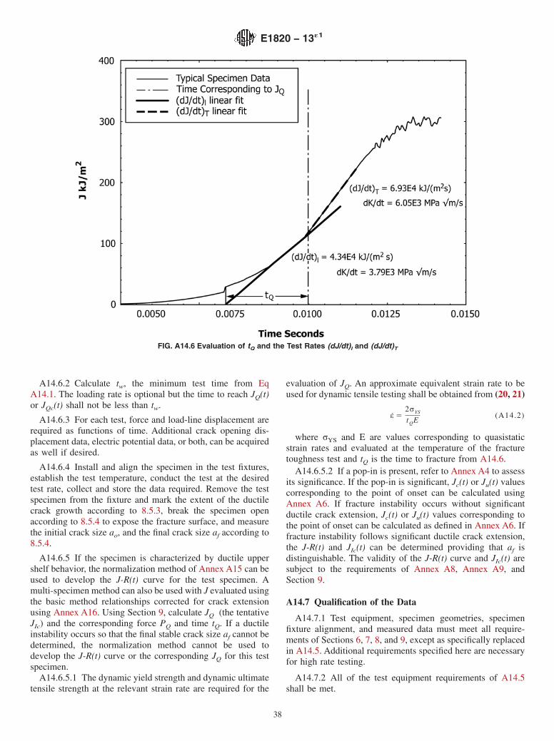
A14.6.2 Calculate tw, the minimum test time from EqA14.1. The loading rate is optional but the time to reach JQ(t)or JQc(t) shall not be less than tw.

A14.6.3 For each test, force and load-line displacement arerequired as functions of time. Additional crack opening dis-placement data, electric potential data, or both, can be acquiredas well if desired.

A14.6.4 Install and align the specimen in the test fixtures,establish the test temperature, conduct the test at the desiredtest rate, collect and store the data required. Remove the testspecimen from the fixture and mark the extent of the ductilecrack growth according to 8.5.3, break the specimen openaccording to 8.5.4 to expose the fracture surface, and measurethe initial crack size ao, and the final crack size af according to8.5.4.

A14.6.5 If the specimen is characterized by ductile uppershelf behavior, the normalization method of Annex A15 can beused to develop the J-R(t) curve for the test specimen. Amulti-specimen method can also be used with J evaluated usingthe basic method relationships corrected for crack extensionusing Annex A16. Using Section 9, calculate JQ (the tentativeJIc) and the corresponding force PQ and time tQ. If a ductileinstability occurs so that the final stable crack size af cannot bedetermined, the normalization method cannot be used todevelop the J-R(t) curve or the corresponding JQ for this testspecimen.

A14.6.5.1 The dynamic yield strength and dynamic ultimatetensile strength at the relevant strain rate are required for the

evaluation of JQ. An approximate equivalent strain rate to beused for dynamic tensile testing shall be obtained from (20, 21)

ε 52σYS

tQE(A14.2)

where σYS and E are values corresponding to quasistaticstrain rates and evaluated at the temperature of the fracturetoughness test and tQ is the time to fracture from A14.6.

A14.6.5.2 If a pop-in is present, refer to Annex A4 to assessits significance. If the pop-in is significant, Jc(t) or Ju(t) valuescorresponding to the point of onset can be calculated usingAnnex A6. If fracture instability occurs without significantductile crack extension, Jc(t) or Ju(t) values corresponding tothe point of onset can be calculated as defined in Annex A6. Iffracture instability follows significant ductile crack extension,the J-R(t) and JIc(t) can be determined providing that af isdistinguishable. The validity of the J-R(t) curve and JIc(t) aresubject to the requirements of Annex A8, Annex A9, andSection 9.

A14.7 Qualification of the Data

A14.7.1 Test equipment, specimen geometries, specimenfixture alignment, and measured data must meet all require-ments of Sections 6, 7, 8, and 9, except as specifically replacedin A14.5. Additional requirements specified here are necessaryfor high rate testing.

A14.7.2 All of the test equipment requirements of A14.5shall be met.

FIG. A14.6 Evaluation of tQ and the Test Rates (dJ/dt)I and (dJ/dt)T

E1820 − 13´1

38

A14.7.3 Plot the J integral versus the time as shown in Fig.A14.6. If fracture instability occurs, calculate J based on a o

using the basic analysis procedure and plot the data up to andincluding JQc(t) or JQu(t). Use a linear regression analysis toevaluate (dJ/dt)I as shown in the example of Fig. A14.5 usingthe data from 0.5JQ(t) to JQ(t), from 0.5JQc(t) to JQc(t), or from0.5 JQu(t) to JQu(t), as the case may be. Extrapolate this line tothe abscissa to evaluate the quantity tQ, as shown in Fig. A14.6.

A14.7.3.1 A second loading rate, (dJ/dt )T, is defined as theslope of the J versus time data beyond maximum force, asshown in Fig. A14.6, over the range from JQ to JQ + 0.5(Jmax

−JQ) or the end of test, if fracture instability occurs.

A14.7.4 Plot force versus load-line displacement for thetime interval 0 ≤ t ≤ tQ, as shown schematically in Fig. A14.7.Use a linear regression analysis to evaluate the initial specimenstiffness ks using data over the range from 20 % to 50 % of themaximum force measured in the test. Plot this best fit line onthe figure, and also plot two parallel lines of the same slopewith the y-intercept offset by 610 % of Pmax as shown in Fig.A14.7. Locate the final crossover ∆LL

F.A14.7.4.1 For this data set to be qualified according to this

method, the compliance, 1/ks, shall agree with the predictionsof Eq A2.10 for the C(T) specimen and Eq A1.10 for the SE(B)specimen within 610 %. Additionally, the measured forcedisplacement data in the region between 0.3∆LL

F and 0.8∆LLF

should remain within the bounds of the parallel lines con-structed on Fig. A14.7. If these requirements are not met, slackgrips or impact absorbers must be added or modified or the testrate reduced to obtain a smoother data set that can be qualifiedaccording to this method.

A14.7.5 If tQ < tw, the test data are not qualified accordingto this method. A slower loading rate must be used, or thespecimen geometry changed to decrease tw for the test to bequalified according to this method.

A14.7.6 If the normalization method of Annex A15 is usedto obtain JIc, the J resistance curve, or both, at least oneconfirmatory specimen must be tested at the same test rate andunder the same test conditions. From the normalization methodthe load-line displacement corresponding to a ductile crackextension of 0.5 mm shall be estimated. The additionalspecimen shall then be loaded to this load-line displacementlevel, marked, broken open and the ductile crack growthmeasured. The measured crack extension shall be 0.5 6 0.25mm in order for these results to be qualified according to thismethod.

A14.8 Qualifying the High Rate Results

A14.8.1 All qualification requirements of 9.1, Annex A6,Annex A8, Annex A9, and A14.7 must be met to qualify theJ-R(t) curve, JQ(t) as JIc(t), or JQc(t) as Jc(t) according to thismethod. If the normalization method of Annex A15 is used, theadditional requirements of this annex shall also be met.

A14.8.2 The maximum crack extension capacity for aspecimen to qualify the J-R(t) curve is given by the following:

∆amax 5 0.15bo (A14.3)

A14.9. Report

A14.9.1 The report shall include all the items of Section 10as well as the following:

A14.9.1.1 The minimum test time, tw, according to A14.6.2.A14.9.1.2 The PQ and tQ, corresponding to the calculated

JQ(t) or JQc(t).A14.9.1.3 The (dJ/dt)I, (dJ/dt)T values, or both.A14.9.1.4 If JIc(t) is being reported, the final crack exten-

sion obtained on the confirmatory specimen of A14.7.6 shall bereported.

FIG. A14.7 Force Smoothness Verification Schematic

E1820 − 13´1

39

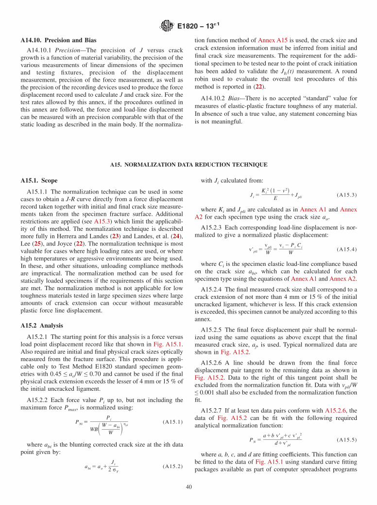
A14.10. Precision and Bias

A14.10.1 Precision—The precision of J versus crackgrowth is a function of material variability, the precision of thevarious measurements of linear dimensions of the specimenand testing fixtures, precision of the displacementmeasurement, precision of the force measurement, as well asthe precision of the recording devices used to produce the forcedisplacement record used to calculate J and crack size. For thetest rates allowed by this annex, if the procedures outlined inthis annex are followed, the force and load-line displacementcan be measured with an precision comparable with that of thestatic loading as described in the main body. If the normaliza-

tion function method of Annex A15 is used, the crack size andcrack extension information must be inferred from initial andfinal crack size measurements. The requirement for the addi-tional specimen to be tested near to the point of crack initiationhas been added to validate the JIc(t) measurement. A roundrobin used to evaluate the overall test procedures of thismethod is reported in (22).

A14.10.2 Bias—There is no accepted “standard” value formeasures of elastic-plastic fracture toughness of any material.In absence of such a true value, any statement concerning biasis not meaningful.

A15. NORMALIZATION DATA REDUCTION TECHNIQUE

A15.1. Scope

A15.1.1 The normalization technique can be used in somecases to obtain a J-R curve directly from a force displacementrecord taken together with initial and final crack size measure-ments taken from the specimen fracture surface. Additionalrestrictions are applied (see A15.3) which limit the applicabil-ity of this method. The normalization technique is describedmore fully in Herrera and Landes (23) and Landes, et al. (24),Lee (25), and Joyce (22). The normalization technique is mostvaluable for cases where high loading rates are used, or wherehigh temperatures or aggressive environments are being used.In these, and other situations, unloading compliance methodsare impractical. The normalization method can be used forstatically loaded specimens if the requirements of this sectionare met. The normalization method is not applicable for lowtoughness materials tested in large specimen sizes where largeamounts of crack extension can occur without measurableplastic force line displacement.

A15.2 Analysis

A15.2.1 The starting point for this analysis is a force versusload point displacement record like that shown in Fig. A15.1.Also required are initial and final physical crack sizes opticallymeasured from the fracture surface. This procedure is appli-cable only to Test Method E1820 standard specimen geom-etries with 0.45 ≤ ao/W ≤ 0.70 and cannot be used if the finalphysical crack extension exceeds the lesser of 4 mm or 15 % ofthe initial uncracked ligament.

A15.2.2 Each force value Pi up to, but not including themaximum force Pmax, is normalized using:

PNi 5Pi

WBS W 2 abi

W D ηpl(A15.1)

where abi is the blunting corrected crack size at the ith datapoint given by:

abi 5 ao1Ji

2 σY

(A15.2)

with Ji calculated from:

Ji 5Ki

2 ~1 2 v2!E

1Jpli (A15.3)

where Ki and Jpli are calculated as in Annex A1 and AnnexA2 for each specimen type using the crack size ao.

A15.2.3 Each corresponding load-line displacement is nor-malized to give a normalized plastic displacement:

v'pli 5vpli

W5

v i 2 Pi Ci

W(A15.4)

where Ci is the specimen elastic load-line compliance basedon the crack size abi, which can be calculated for eachspecimen type using the equations of Annex A1 and Annex A2.

A15.2.4 The final measured crack size shall correspond to acrack extension of not more than 4 mm or 15 % of the initialuncracked ligament, whichever is less. If this crack extensionis exceeded, this specimen cannot be analyzed according to thisannex.

A15.2.5 The final force displacement pair shall be normal-ized using the same equations as above except that the finalmeasured crack size, af, is used. Typical normalized data areshown in Fig. A15.2.

A15.2.6 A line should be drawn from the final forcedisplacement pair tangent to the remaining data as shown inFig. A15.2. Data to the right of this tangent point shall beexcluded from the normalization function fit. Data with vpli/W≤ 0.001 shall also be excluded from the normalization functionfit.

A15.2.7 If at least ten data pairs conform with A15.2.6, thedata of Fig. A15.2 can be fit with the following requiredanalytical normalization function:

PN 5a1b v'pl1c v'pl

2

d1v'pl

(A15.5)

where a, b, c, and d are fitting coefficients. This function canbe fitted to the data of Fig. A15.1 using standard curve fittingpackages available as part of computer spreadsheet programs

E1820 − 13´1

40

or separately. An example fit for the data of Fig. A15.2 is shown in Fig. A15.3. The normalization function shall fit all

FIG. A15.1 Typical Force versus Displacement Curve

FIG. A15.2 Normalized Force versus Displacement Curve Showing Points up to Maximum Force and the Final Data Point

E1820 − 13´1

41

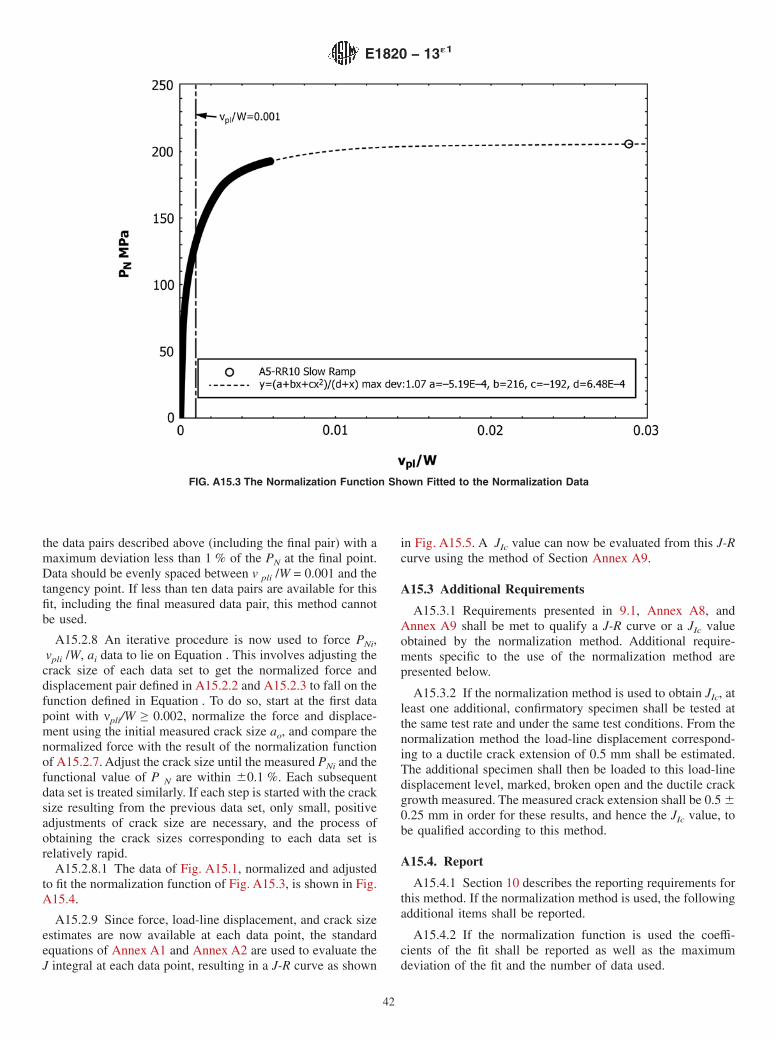
the data pairs described above (including the final pair) with amaximum deviation less than 1 % of the PN at the final point.Data should be evenly spaced between v pli /W = 0.001 and thetangency point. If less than ten data pairs are available for thisfit, including the final measured data pair, this method cannotbe used.

A15.2.8 An iterative procedure is now used to force PNi,vpli /W, ai data to lie on Equation . This involves adjusting thecrack size of each data set to get the normalized force anddisplacement pair defined in A15.2.2 and A15.2.3 to fall on thefunction defined in Equation . To do so, start at the first datapoint with νpli/W ≥ 0.002, normalize the force and displace-ment using the initial measured crack size ao, and compare thenormalized force with the result of the normalization functionof A15.2.7. Adjust the crack size until the measured PNi and thefunctional value of P N are within 60.1 %. Each subsequentdata set is treated similarly. If each step is started with the cracksize resulting from the previous data set, only small, positiveadjustments of crack size are necessary, and the process ofobtaining the crack sizes corresponding to each data set isrelatively rapid.

A15.2.8.1 The data of Fig. A15.1, normalized and adjustedto fit the normalization function of Fig. A15.3, is shown in Fig.A15.4.

A15.2.9 Since force, load-line displacement, and crack sizeestimates are now available at each data point, the standardequations of Annex A1 and Annex A2 are used to evaluate theJ integral at each data point, resulting in a J-R curve as shown

in Fig. A15.5. A JIc value can now be evaluated from this J-Rcurve using the method of Section Annex A9.

A15.3 Additional Requirements

A15.3.1 Requirements presented in 9.1, Annex A8, andAnnex A9 shall be met to qualify a J-R curve or a JIc valueobtained by the normalization method. Additional require-ments specific to the use of the normalization method arepresented below.

A15.3.2 If the normalization method is used to obtain JIc, atleast one additional, confirmatory specimen shall be tested atthe same test rate and under the same test conditions. From thenormalization method the load-line displacement correspond-ing to a ductile crack extension of 0.5 mm shall be estimated.The additional specimen shall then be loaded to this load-linedisplacement level, marked, broken open and the ductile crackgrowth measured. The measured crack extension shall be 0.5 6

0.25 mm in order for these results, and hence the JIc value, tobe qualified according to this method.

A15.4. Report

A15.4.1 Section 10 describes the reporting requirements forthis method. If the normalization method is used, the followingadditional items shall be reported.

A15.4.2 If the normalization function is used the coeffi-cients of the fit shall be reported as well as the maximumdeviation of the fit and the number of data used.

FIG. A15.3 The Normalization Function Shown Fitted to the Normalization Data

E1820 − 13´1

42

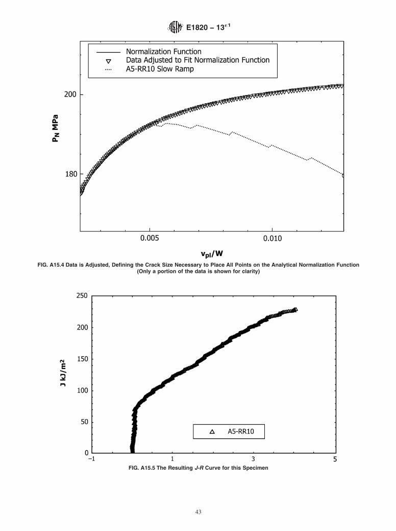
FIG. A15.4 Data is Adjusted, Defining the Crack Size Necessary to Place All Points on the Analytical Normalization Function(Only a portion of the data is shown for clarity)

FIG. A15.5 The Resulting J-R Curve for this Specimen

E1820 − 13´1

43

A15.4.3 If JIc is reported, the accuracy of the confirmatoryspecimen of A15.3.2 shall be reported.

A15.5. Precision and Bias

A15.5.1 Precision—The precision of the J resistance curveis a function of material variability, the precision of the variousmeasurements of linear dimensions of the specimen and testingfixtures, precision of the displacement measurement, precisionof the force measurement, as well as the precision of therecording devices used to produce the force displacementrecord used to calculate J and crack size. For the test ratesallowed by this annex, if the procedures outlined in this annexare followed, the crack size throughout the fracture toughnesstest can be measured with a precision comparable with that ofthe unloading compliance procedure described in the mainbody. A round robin describing the use of the normalizationprocedure on rapidly loaded SE(B) and C(T) specimens ispresented in (22). A requirement for the testing of a confirma-

tory specimen tested near the point of stable crack initiation ispresent to validate the JIc measurement.

A15.5.2 Bias—Crack sizes generally vary through the thick-ness of fracture toughness specimens. A nine point averageprocedure based on optical measurements obtained from thepost-test fracture surface is generally used to give a reportablecrack size. Different measurements would be obtained usingmore or less measurement points. Alternative crack sizes canbe estimated using compliance methods, which obtain differentaverage crack size estimates for irregular crack front shapes.Stringent crack front straightness requirements are present inthis standard to minimize differences caused by these effects.The normalization method acts to interpolate between opticallymeasured crack average lengths measured at the start and endof the stable resistance curve fracture toughness test. Thismethod has been demonstrated in (22) to give results consistentwith those obtained by unloading compliance procedures.

A16. EVALUATION OF CRACK GROWTH CORRECTED J-INTEGRAL VALUES

A16.1 J Correction Procedure :

A16.1.1 Evaluate Jel0 and Jpl0 values for each specimenusing the basic method equations of Annex A1 – Annex A3 forthe specimen type.

A16.1.2 Obtain initial crack growth corrected J values usingthe following relationship (26) :

J 5 Jel01Jpl0

11S α 2 0.5α10.5 D ∆a

bo

(A16.1)

with α = 1 for SE(B) specimens and α = 0.9 for C(T) andDC(T) specimens.

A16.1.3 Fit a power law expression J = J1mm∆am to thecorrected J(∆a) data for crack growths exceeding ∆a/bo ≥ 0.05.

A16.1.4 Calculate the final crack growth corrected J(∆a)data using:

J 5 Jel01Jpl0

11S α 2 mα1m D ∆a

bo

(A16.2)

A17. FRACTURE TOUGHNESS TESTS AT IMPACT LOADING RATES USING PRECRACKED CHARPY-TYPE SPECIMENS

A17.1 Scope

A17.1.1 This Annex specifies requirements for performingand evaluating instrumented impact tests on precrackedCharpy-type specimens using a fracture mechanics approach.Minimum requirements are given for measurement and record-ing equipment such that similar sensitivity and comparablemeasurements are achieved. Dynamic fracture mechanicsproperties determined are comparable to conventional large-scale fracture mechanics results when the validity criteria ofAnnex A8-Annex A11 and Annex A14 are met. However,because of the small absolute size of the Charpy specimen, thisis often not the case. Nevertheless, the values obtained can beused in research and development of materials, in qualitycontrol and service evaluation and to establish the relativevariation of properties with test temperature and loading ratemeasured on precracked Charpy-type specimens.

A17.2 Principle

A17.2.1 This Annex prescribes impact bend tests which areperformed on fatigue precracked Charpy-type specimens toobtain dynamic fracture mechanics properties of materials.This Annex extends the procedure for V-notch impact bendtests in accordance with Test Methods E23, and may be usedfor evaluation of the Master Curve in accordance with TestMethod E1921. Instrumented testing machines are required inorder to utilize this Annex, together with ancillary instrumen-tation and recording equipment in accordance with TestMethod E2298. The characteristic fracture toughness param-eters depend on material response reflected in the force/timediagrams described in Table A17.1 and Fig. A17.1. Note thatonly Type I diagrams can be linearly fit up to fracture.

NOTE A17.1—The symbol used in these Test Methods for force is P,while Test Method E2298 uses F. Therefore the parameters Pmax , Pbf, Pgy

E1820 − 13´1

44

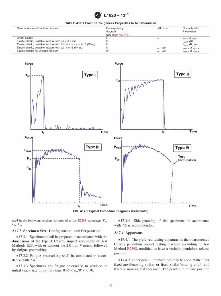
used in the following sections correspond to the E2298 parameters Fm,Fbf, Fgy.

A17.3 Specimen Size, Configuration, and Preparation

A17.3.1 Specimens shall be prepared in accordance with thedimensions of the type A Charpy impact specimens of TestMethods E23, with or without the 2.0 mm V-notch, followedby fatigue precracking.

A17.3.2 Fatigue precracking shall be conducted in accor-dance with 7.4.

A17.3.3 Specimens are fatigue precracked to produce aninitial crack size ao in the range 0.45 < ao/W < 0.70.

A17.3.4 Side-grooving of the specimens in accordancewith 7.5 is recommended.

A17.4 Apparatus

A17.4.1 The preferred testing apparatus is the instrumentedCharpy pendulum impact testing machine according to TestMethod E2298, modified to have a variable pendulum releaseposition.

A17.4.2 Other pendulum machines may be used, with eitherfixed anvil/moving striker or fixed striker/moving anvil, andfixed or moving test specimen. The pendulum release position

TABLE A17.1 Fracture Toughness Properties to be Determined

Material response/fracture behavior Correspondingdiagramtype (See Fig. A17.1)

J-R curve CharacteristicParameters

Linear-elastic I ... JcdX, KJcd,X

Elastic-plastic, unstable fracture with ∆a < 0.2 mm II ... Jcd,X (B)Elastic-plastic, unstable fracture with 0.2 mm # ∆a # 0.15 (W–a0) II ... Jud,X (B, ∆a)Elastic-plastic, unstable fracture with ∆a $ 0.15 (W–a0) III Jd –∆a JQd,X or JIcd,X

Elastic plastic; no unstable fracture IV Jd –∆a JQd,X or JIcd,X

FIG. A17.1 Typical Force-time Diagrams (Schematic)

E1820 − 13´1

45

for such machines is normally variable, and the striker or anvilsare normally instrumented to provide force/time or force/displacement records.

A17.4.3 Falling weight testing machines, which may bespring assisted, are allowed. The striker is normally instru-mented to provide force/time or force/time and force/displacement records.

A17.4.4 Other testing machines which comply with thecalibration and other requirements of Test Method E2298 arenot excluded.

A17.4.5 Requirements on Absorbed Energy—The reliabilityof instrumented force values on which these tests are baseddepends on the quality of the acquisition system and thecalibration of the instrumented striker. The calibration of thestriker shall be performed in accordance with Test MethodE2298. Additionally, for each test in which the entire forcesignal has been recorded (that is, until the force returns to thebaseline), one of the following requirements shall be met:

(a) the difference between KV and Wt shall be within615 % of KV or 61 J, whichever is larger, or

(b) the difference between KV and Wt shall not exceed625 % or 62 J, whichever is larger.

For every test that fulfills requirement (b), but not (a), forcevalues may be adjusted using an iterative procedure until theequivalence KV = Wt is achieved (27). If the difference betweenKV and Wt exceeds 625 % of KV or 62 J, whichever is larger,the test shall be discarded and the user shall check and ifnecessary repeat the instrumented striker calibration. If record-ing of the entire force signal for an individual test is notachieved (for example due to the specimen being ejected fromthe machine without being fully broken), the user shalldemonstrate conformance of the testing system using at leastfive specimens of the same test series, for which the entireforce signal has been recorded, that fulfil one of the aboverequirements. Otherwise, conformance shall be demonstratedby testing at least five additional non-precracked or precrackedCharpy specimens, and showing that in all cases the differencebetween KV and Wt is within 615 % of KV or 61 J, whicheveris larger. If this requirement is not met but the differencebetween KV and Wt does not exceed 625 % of KV or 62 J, theforce adjustment described above shall be applied.

NOTE A17.2—From a theoretical point of view, KV is expected to beslightly higher than Wt, the difference being due to vibrational energylosses and other smaller contributions such as secondary impacts betweenstriker and specimen. For more insight on the difference between KV andWt, see reference (28).

A17.5 Test Procedures and Measurements

A17.5.1 Tests are performed in a manner similar to thestandard Charpy impact test of Test Methods E23 and theinstrumented impact test of Test Method E2298, especiallywith regard to the pendulum hammer and the handling ofpre-cooled or pre-heated specimens.

A17.5.2 Data recording—The force/displacement diagramis recorded according to Test Method E2298, from which thekey data values Pmax , Pbf, Wm, and Wt are determined. Inaddition to the procedures of Test Method E2298, the following

procedures are provided concerning impact velocity, availableenergy and time to fracture. These data form the basis forevaluation of toughness parameters according to A17.6-A17.9.

A17.5.2.1 Impact velocity and available energy—This stan-dard applies to any impact velocity v0, provided the time tofracture fulfills the requirements of A17.5.2.2. Impact veloci-ties for pendulum or falling weight testing machines can bevaried by adjusting the striker release height. The impactvelocity v0 for a pendulum machine can be determined asfollows: set the pointer to the end-of-scale position as in aconventional Charpy test per Test Methods E23, release thependulum from the appropriately reduced height, with nospecimen in place. Read the energy KV0 (in J) indicated by thepointer on the analogue scale. From this, the correspondingimpact velocity is calculated as:

vo 5 vosŒMC 2 KV0

MC(A17.1)

where vos is the maximum pendulum velocity correspondingto MC, the full pendulum capacity. A reduced velocity (1 to2 m/s) can be advantageous, especially for brittle materials,since it reduces the effect of oscillations by lowering theirrelative amplitude and by increasing their number within thefracture time tf (see A17.5.2.2).

A17.5.2.2 Time to fracture—When the time tf to initiateunstable fracture is less than the minimum test time tw ofA14.3.1.4, the instant of crack initiation is not detectable in theforce signal with adequate accuracy because of oscillations(see Fig. A17.1 - Type I), and fracture toughness cannot beevaluated using this test method.

A17.5.3 Recording Apparatus—Refer to Section 7 of TestMethod E2298.

A17.5.4 Execution of the Test—Refer to Section 9 of TestMethod E2298.

A17.5.5 Evaluation of the Force-Displacement Curve—Refer to Section 11 of Test Method E2298.

A17.5.6 Calculation of fracture parameters— The value ofJ-integral at unstable fracture, Jcd (force-time diagrams Type Iand II in Fig. A17.1) or Jud (force-time diagram of Type III inFig. A17.1), or at test termination, Jd (force-time diagram ofType IV in Fig. A17.1) shall be calculated using the appropriateformulas Eq A1.4-A1.6 for the Basic Test Method. Inparticular, the specimen elastic compliance C0 is required toevaluate the plastic component of the area under the force-displacement curve (Fig. A1.2). This can be obtained using thefollowing theoretical expression:

C0,th 5 CS1CM (A17.2)where CS is the specimen compliance calculated using EqA1.10 and CM is the impact machine compliance. This lattercan be measured with unnotched specimens using one of themethods described in (29). Alternatively, if CM is notavailable, C0 can be estimated as the reciprocal of the initialelastic slope (C0,exp ), by fitting force-displacement data be-tween the second oscillation (that is, discarding the first iner-tia peak) and the onset of general yielding. If both C0,exp andC0,th are available, C0,th shall be used and the difference be-tween the two values shall be within 615 %. Values of

E1820 − 13´1

46

stress intensity factor shall be obtained from the correspond-ing J-integral values using:

KJd 5ΠEJd

1 2 v2 (A17.3)

Calculated KJd values at the onset of cleavage fracture, KJcd,can be used to calculate the reference temperature, T0, inaccordance with Test Method E1921, provided all relevantrequirements are met.

A17.5.7 Crack Size Measurements—Original crack size andfinal physical crack size shall be measured in accordance with8.5.

A17.5.8 Multiple Specimen Tests—To determine dynamicJ-R curves by multi-specimen techniques, the fracture processis interrupted over a range of stable crack extension values, thatare combined to obtain a single J-R curve. This procedure isdescribed in A17.7.

A17.5.9 Single Specimen Tests—It is also possible to esti-mate dynamic J-R curves from an individual specimen usingthe Normalization Data Reduction technique, as described inA17.8.

A17.6 Analysis of Results

A17.6.1 Fracture Behavior—The adequacy of fracturetoughness parameters depends on the fracture behavior of thetest specimen as reflected in the force-displacement diagramsdescribed in Table A17.1. Therefore the measured force dis-placement or force-time diagram shall be assigned to one of thediagram types shown in Fig. A17.1, using the indicationsprovided in Table A17.1.

A17.6.2 Unstable Fracture—In the case of unstable fractureas in Fig. A17.1 - Types I or II, the applicable evaluationmethod depends on the oscillations superimposed on the forcesignal. If time to fracture is more than the minimum test timeof A14.3.1.4, fracture toughness shall be evaluated accordingto the quasi-static approach of Annex A6 and Annex A7.Impact velocity may be reduced in order for the time to fractureto fulfil the requirements of A14.3.1.4 and A17.5.2.

A17.6.3 Stable Crack Extension—In the case of stable crackextension as in Fig. A17.1 - Types III or IV, either multispecimen or single-specimen techniques described in A17.7and A17.8, respectively, are to be used to determine the J Rcurve. The determination of characteristic fracture toughnessvalues from dynamic J-R curves is described in A17.9.

A17.6.4 Loading Rate— As indicated in Table A17.1, frac-ture toughness values shall be stated with the correspondingloading rate added in parentheses. The latter may be estimatedas follows:Type I:

K 5KJcd

t f

(A17.4)

Types I and II:

J 5Jcd

t f

(A17.5)

or

J 5Jud

t f

Types III and IV:

J 5Pmax·vo

BN·~W 2 ao!·ηplS ao

W D (A17.6)

In alternative to Eq A17.6, the procedures given in A14.7.3and A14.7.3.1 can also be used for calculating (dJ/dt)I and(dJ/dt)T respectively. For practical purposes, the loading rateshall be indicated using its order of magnitude (for example,the stress intensity factor corresponding to a loading rate of4 × 105 MPa√m/s shall be indicated as KJcd5).

A17.6.5 Dynamic Tensile Properties— The dynamic yieldand ultimate tensile stresses at the relevant strain rate may berequired for certain evaluation procedures and validity checks.An approximate equivalent strain rate for the fracture mechan-ics test, which can be used for dynamic tensile testing, may becalculated from (20, 21):

ε 5 2σYS

t ·E(A17.7)

where: σYS and E are values corresponding to quasistaticstrain rates (that is, conforming to the requirements of TestMethods E8/E8M) and evaluated at the temperature of thefracture mechanics test; t is the time to fracture in the caseof small scale yielding (type I in Fig. A17.1), or the timeinterval of the initial linear part of the force-time record inthe case of distinct elastic-plastic material behavior (typesII-IV in Fig. A17.1). Eq A17.7 provides a general estimateof strain rate values associated with fracture in the testspecimen.

A17.7 Determination of J-R curves at Impact LoadingRates by Multiple Specimen Methods

A17.7.1 The following methods make it possible to deter-mine fracture toughness parameters in those cases where stablecrack extension occurs, Fig. A17.1 – Types III and IV. Themulti-specimen procedure involves loading a series of nomi-nally identical specimens to selected displacement levels,resulting in corresponding amounts of stable crack extension.Each specimen tested provides one point on the resistancecurve. The requirements and procedures of Annex A8-AnnexA11 concerning number and spacing of data points shall befulfilled.

A17.7.2 Low-blow Test—This test procedure is intended tolimit the impact energy W0 of the pendulum hammer or dropweight so that it is sufficient to produce a certain stable crackextension, but not sufficient to fully break the specimen. Byselecting different energy levels in a series of tests on nomi-nally identical specimens, a series of different crack extensions∆ai are produced. From the corresponding J-values, J-∆acurves are constructed.

NOTE A17.3—An alternative method is the Stop Block approach,whereby the hammer swing is arrested by using stop blocks, thus avoidingcomplete fracture of the specimen.

A17.7.2.1 The following procedure is recommended:(1) Prepare 7 – 10 specimens to nominally the same initial

crack length a0.(2) Perform a full blow instrumented impact bending test

on one of the specimens. Evaluate the energy at maximum

E1820 − 13´1

47

force and the total fracture energy, Wm and Wt, in accordancewith Test Method E2298.

(3) Determine the energy spacing as ∆W0 = 2Wm/N, whereN is the number of available specimens.

(4) Perform an impact test by setting the release position ofthe pendulum hammer, or the height of the drop weight, suchthat W0 = 2Wm/N. Avoid a second impact between the strikerand the test specimen.

(5) Repeat the test on the remaining specimens, increasingthe impact energy W0 by the amount ∆W0 =2Wm/N at each test.

(6) In order to mark the crack extension, post-test fatiguecycling or heat tinting may be used.

(7) Break all specimens open after testing. Care is to betaken to minimize post-test specimen deformation. Coolingferritic steels may help to ensure brittle behavior duringspecimen opening.

(8) Measure a0 and ∆ap = ∆ai (where “i” is the test index,with 1 ≤ i ≤ N-1) in accordance with 8.5.

(9) Calculate Ji according to A1.4.2.1.(10) Plot the resulting N-1 pairs of values (Ji, ∆ai ) in a J-∆a

diagram and determine the J-R curve according to Annex A8and JQd,X (a provisional value of JIcd,X) according to Annex A9.

A17.7.2.2 The differences in impact velocity and loadingrate between the various tests are small enough to have anegligible influence on the results and can be ignored, providedvelocity and loading rate do not vary by more than a factor 3between the minimum and maximum values.

A17.7.3 Cleavage J-R curve Method—This test method canonly be used for steels that exhibit a brittle-ductile transition.The test temperature is varied within the ductile-to-brittletransition zone so that stable crack extensions of varyinglengths ∆ap are obtained from tests terminated by cleavagefracture. Jud values calculated according to A1.4.2 and thecorresponding ∆ap represent points on the cleavage J-∆a curvewhich can be analyzed in accordance with Annex A8 andAnnex A9. Differences between the temperatures of the variousresistance points can be neglected, provided they don’t exceed50 °C. The requirements of Annex A8 and Annex A9 shall besatisfied in order to obtain a valid J-R curve. Details of thismethod are given in (30).

A17.7.4 The user is warned that results obtained using theLow-blow or Stop Block methods, in which the loading rate isprogressively reduced down to zero, may differ from resultsobtained using tests leading to specimen fracture, such as theCleavage J-R curve method.

A17.8 J-R Curve Determination by Single Specimen Meth-ods

A17.8.1 The Normalization Data Reduction (NDR) tech-nique can be applied to a Low-blow test performed inaccordance with A17.7.1, provided the measured crack exten-sion does not exceed 15 % of the initial uncracked ligament.The provisions of Annex A15 apply, including the additionalrequirements of A15.3. A study published in (31) shows thatfor two steels and two test temperatures, NDR single-specimenresults are in good agreement with multiple specimen datagenerated using the Low-blow technique.

A17.9 Determination of Fracture Toughness Near the On-set of Stable Crack Extension

A17.9.1 From J-R curves determined according to A17.7 orA17.8, fracture toughness values near the onset of stable crackextension can be determined in conformance to Annex A9.Specimen qualification as per Annex A9 requirements will bedifficult to achieve if the specimen undergoes significantplasticity during crack extension because of the relatively smallsize of the specimen. In this case, values of JQd cannot beregarded as material properties independent of specimen sizeand their use in safety assessments may result in non conser-vative results. Nevertheless, these values can be used forresearch and development of materials, in quality control andservice evaluation and to establish the variation of propertieswith test temperature.

A17.9.2 The construction line for JQ calculation shall havethe following expression, see also Eq A9.4:

J 5 2σFSd∆a (A17.8)where σFSd, the dynamic flow strength, is the average of thedynamic yield strength and the dynamic ultimate tensilestrength:

σFSd 5σYSd1σTSd

2(A17.9)

σYSd and σTSd shall preferably be obtained from dynamictensile tests, provided that it can be demonstrated that thecorresponding strain rate is equivalent to that of the fracturetoughness tests (see A17.6.5). Alternatively, estimated valuescan be obtained from the force/displacement test record of theimpact test as (32):

σYSd 52.732Pgy W

~W 2 a0!2 BN

(A17.10)

and

σTSd 52.732Pmax W

~W 2 a0!2 BN

(A17.11)

NOTE A17.4—For plane-sided specimens, BN = B.

A17.10 Report

A17.10.1 In addition to the information listed in Section 10of the main body, the test report shall include the following.

A17.10.2 Identification and type of testing apparatus.

A17.10.3 Striker impact velocity vo (A17.5.3).

A17.10.4 Nominal energy of the striker at velocity vo.

A17.10.5 Absorbed energy KV according to Test MethodE2298.

A17.10.6 Calibration of the instrumented striker.

A17.10.7 Details of force adjustment in accordance withA17.4.5, if applicable.

A17.10.8 Specimen elastic compliance (theoretical orexperimental, or both) and, if available, machine compliance.

A17.10.9 Time to fracture or time at test termination, asappropriate.

A17.10.10 Fracture parameters determined as:(1) value of KJcd obtained, if applicable,

E1820 − 13´1

48

(2) value of K obtained, if applicable (only order ofmagnitude),

(3) value of J obtained, if applicable,(4) value of J obtained, if applicable (only order of

magnitude),(5) type of force-time diagram, with reference to Fig.

A17.1, Types I – IV,

(6) for diagrams of Types III or IV, final crack extension,and

(7) a copy of the test record.

A17.10.11 In case of J-R curve determination, values of Jand ∆a in tabular form and values of JQd,X or JIcd,X obtained.

A17.10.12 Dynamic tensile properties used, if applicable.

APPENDIXES

(Nonmandatory Information)

X1. FITTING OF EQUATION A9.1

X1.1 To fit Eq A9.1 to the Ji, ai data using the method ofleast squares, the following equation must be set up and solvedfor aoq, B, and C:

X1.2 This equation can be set up and solved using astandard spreadsheet or using a mathematical analysis programlike MathCad, Maple, or Mathematica.

X2. GUIDELINES FOR MEASURING THE FRACTURE TOUGHNESS OF MATERIALS WITH SHALLOW CRACKS

X2.1 Significance and Use

X2.1.1 Fracture toughness measurements may be madeusing specimens with relatively shallow cracks, 0.05 < a/W <0.45, which are not permitted by the standard test method. Theresulting measures of fracture toughness, designated JxSC() andδxSC(), will be dependent upon the size of the specimen and thecrack length. The fracture toughness determined from speci-mens with shallow cracks is usually non-conservative whencompared to the fracture toughness determined from standard,deep crack specimen geometries and may exhibit considerablymore scatter, particularly in the ductile to brittle transitionregion for ferritic materials. The J resistance curves determinedaccording to this appendix are not corrected for crack growthand will be non-conservative relative to crack growth correctedresistance curves.

X2.1.2 This appendix is provided to give recommendedprocedures for conducting fracture toughness tests of speci-mens containing shallow cracks. Special requirements for theinstrumentation, specimen, testing procedure and data analysisare described.

X2.1.3 Particular care must be exercised when using thesenon-standard measures of fracture toughness for structuralintegrity assessments. The user is cautioned that differencesmay exist between laboratory test and field conditions and that

the fracture toughness of a shallow crack specimen may bestrongly influenced by the size of the crack and the specimengeometry.

X2.2 Terminology

X2.2.1 All of the following parameters describe variousmeasures of fracture toughness determined using specimenscontaining shallow cracks. These parameters are similar to thecorresponding parameters for standard specimens except thatthey include the subscript SC(a0/W) to indicate a shallow crackspecimen. The number in the parentheses is the original cracksize to specimen width ratio for the shallow crack specimen.

X2.2.1.1 δIcSC() [L]— is a value of CTOD near the onset ofslow stable crack extension in a specimen with a shallow crack,here defined as occurring at ∆ap=0.2 mm (0.008 in) + 0.7δIc.

X2.2.1.2 δSC() [L]—is the value of CTOD at the onset ofunstable crack extension (see 3.2.39) or pop-in (see 3.2.25) ina specimen with a shallow crack when ∆ap<0.2 mm (0.008 in)+ 0.7δcSC(). δcSC() corresponds to the force Pc and clip-gagedisplacement vc (see Fig. 1).

X2.2.1.3 δuSC()[L]—is the value of CTOD at the onset ofunstable crack extension (see 3.2.39) or pop-in (see 3.2.25) ina specimen with a shallow crack when the event is preceded by∆ap≥0.2 mm (0.008 in) + 0.7δuSC(). δuSC() corresponds to theforce Pu and the clip gage displacement vu (see Fig. 1). It may

E1820 − 13´1

49

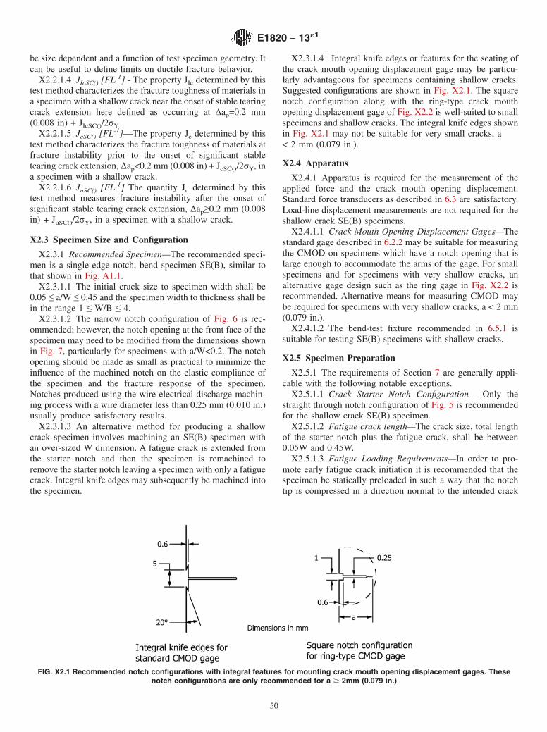
be size dependent and a function of test specimen geometry. Itcan be useful to define limits on ductile fracture behavior.

X2.2.1.4 JIcSC() [FL-1] - The property JIc determined by thistest method characterizes the fracture toughness of materials ina specimen with a shallow crack near the onset of stable tearingcrack extension here defined as occurring at ∆ap=0.2 mm(0.008 in) + JIcSC()/2σY .

X2.2.1.5 JcSC() [FL-1]—The property Jc determined by thistest method characterizes the fracture toughness of materials atfracture instability prior to the onset of significant stabletearing crack extension, ∆ap<0.2 mm (0.008 in) + JcSC()/2σY, ina specimen with a shallow crack.

X2.2.1.6 JuSC() [FL-1] The quantity Ju determined by thistest method measures fracture instability after the onset ofsignificant stable tearing crack extension, ∆ap≥0.2 mm (0.008in) + JuSC()/2σY, in a specimen with a shallow crack.

X2.3 Specimen Size and Configuration

X2.3.1 Recommended Specimen—The recommended speci-men is a single-edge notch, bend specimen SE(B), similar tothat shown in Fig. A1.1.

X2.3.1.1 The initial crack size to specimen width shall be0.05 ≤ a/W ≤ 0.45 and the specimen width to thickness shall bein the range 1 ≤ W/B ≤ 4.

X2.3.1.2 The narrow notch configuration of Fig. 6 is rec-ommended; however, the notch opening at the front face of thespecimen may need to be modified from the dimensions shownin Fig. 7, particularly for specimens with a/W<0.2. The notchopening should be made as small as practical to minimize theinfluence of the machined notch on the elastic compliance ofthe specimen and the fracture response of the specimen.Notches produced using the wire electrical discharge machin-ing process with a wire diameter less than 0.25 mm (0.010 in.)usually produce satisfactory results.

X2.3.1.3 An alternative method for producing a shallowcrack specimen involves machining an SE(B) specimen withan over-sized W dimension. A fatigue crack is extended fromthe starter notch and then the specimen is remachined toremove the starter notch leaving a specimen with only a fatiguecrack. Integral knife edges may subsequently be machined intothe specimen.

X2.3.1.4 Integral knife edges or features for the seating ofthe crack mouth opening displacement gage may be particu-larly advantageous for specimens containing shallow cracks.Suggested configurations are shown in Fig. X2.1. The squarenotch configuration along with the ring-type crack mouthopening displacement gage of Fig. X2.2 is well-suited to smallspecimens and shallow cracks. The integral knife edges shownin Fig. X2.1 may not be suitable for very small cracks, a< 2 mm (0.079 in.).

X2.4 Apparatus

X2.4.1 Apparatus is required for the measurement of theapplied force and the crack mouth opening displacement.Standard force transducers as described in 6.3 are satisfactory.Load-line displacement measurements are not required for theshallow crack SE(B) specimens.

X2.4.1.1 Crack Mouth Opening Displacement Gages—Thestandard gage described in 6.2.2 may be suitable for measuringthe CMOD on specimens which have a notch opening that islarge enough to accommodate the arms of the gage. For smallspecimens and for specimens with very shallow cracks, analternative gage design such as the ring gage in Fig. X2.2 isrecommended. Alternative means for measuring CMOD maybe required for specimens with very shallow cracks, a < 2 mm(0.079 in.).

X2.4.1.2 The bend-test fixture recommended in 6.5.1 issuitable for testing SE(B) specimens with shallow cracks.

X2.5 Specimen Preparation

X2.5.1 The requirements of Section 7 are generally appli-cable with the following notable exceptions.

X2.5.1.1 Crack Starter Notch Configuration— Only thestraight through notch configuration of Fig. 5 is recommendedfor the shallow crack SE(B) specimen.

X2.5.1.2 Fatigue crack length—The crack size, total lengthof the starter notch plus the fatigue crack, shall be between0.05W and 0.45W.

X2.5.1.3 Fatigue Loading Requirements—In order to pro-mote early fatigue crack initiation it is recommended that thespecimen be statically preloaded in such a way that the notchtip is compressed in a direction normal to the intended crack

FIG. X2.1 Recommended notch configurations with integral features for mounting crack mouth opening displacement gages. Thesenotch configurations are only recommended for a $ 2mm (0.079 in.)

E1820 − 13´1

50

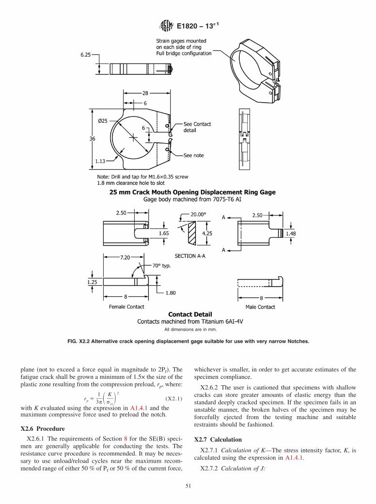
plane (not to exceed a force equal in magnitude to 2Pf). Thefatigue crack shall be grown a minimum of 1.5× the size of theplastic zone resulting from the compression preload, rp, where:

rp 51

3π S Kσys

D 2

(X2.1)

with K evaluated using the expression in A1.4.1 and themaximum compressive force used to preload the notch.

X2.6 Procedure

X2.6.1 The requirements of Section 8 for the SE(B) speci-men are generally applicable for conducting the tests. Theresistance curve procedure is recommended. It may be neces-sary to use unload/reload cycles near the maximum recom-mended range of either 50 % of Pf or 50 % of the current force,

whichever is smaller, in order to get accurate estimates of thespecimen compliance.

X2.6.2 The user is cautioned that specimens with shallowcracks can store greater amounts of elastic energy than thestandard deeply cracked specimen. If the specimen fails in anunstable manner, the broken halves of the specimen may beforcefully ejected from the testing machine and suitablerestraints should be fashioned.

X2.7 Calculation

X2.7.1 Calculation of K—The stress intensity factor, K, iscalculated using the expression in A1.4.1.

X2.7.2 Calculation of J:

All dimensions are in mm.

FIG. X2.2 Alternative crack opening displacement gage suitable for use with very narrow Notches.

E1820 − 13´1

51

X2.7.2.1 J Calculation for the Basic Method— J is calcu-lated according to A1.4.2 except that the crack growth correc-tion of Annex A16 shall not be employed because it is notapplicable to shallow cracks.

X2.7.2.2 J Calculations for the Resistance Curve Method—At a point corresponding tov

~i!, P

~i!on the force versus crack-

mouth opening displacement record, calculate J as follows:

J 5K

~i!2 ~1 2 ν2!

E1Jpl (X2.2)

where K(i) is from A1.4.1 and

Jpl~i!5 Jpl~i21!

1ηCMOD~i21! @ACMODpl~i!

2 ACMODpl~i21!#BNb

~i21!

(X2.3)

In Eq X2.3, the quantity ACMODpl(i) - ACMODpl(i-1) is theincrement of area under the force versus plastic component ofCMOD record between lines of constant displacement at i-1and i as shown in Fig. A1.3. The quantity ACMODpl(i) can beevaluated from the following equation:

ACMODpl~i!5 ACMODpl~i21!

1~Pi1Pi21!

2 ~vpl~i!2 vpl~i21!! (X2.4)

where:vpl(i) = plastic part of the CMOD = v(i)- PiCi andCi = slope (∆vm/∆P)i of the current unload/reload cycle.

In Eq X2.3, ηCMOD is a function of crack size and is givenby the following expression:

ηCMOD ~i21!5 3.667 2 2.199 S a

w D10.437 S aw D 2

(X2.5)

X2.7.2.3 For a resistance curve test method using an elasticcompliance technique with crack mouth opening displacementmeasured at the notched edge of a shallow crack specimen with0.05 ≤ a/W ≤ 0.45, the crack length is given as follows (33):

aW

5 1.01878 2 4.5367u19.0101u2 2 27.333u3174.4u4 2 71.489u5

(X2.6)

where:u = 1

F BeWECi

S/4 G 1/2

11

Ci = (∆vm/∆P) on an unloading/reloading sequence, andBe = = B - (B-BN)2/B

X2.7.3 Calculation of CTOD:

X2.7.3.1 For the shallow crack SE(B) specimen, calcula-tions of CTOD for any point on the force-displacement recordare made using A1.4.5 except that J values shall not be crackgrowth corrected when using equations Eq A1.14 or Eq A1.16.

X2.8 Analysis of Results

X2.8.1 The data shall meet the following requirements to bequalified according to this method. If the data do not pass theserequirements no fracture toughness measures can be deter-mined according to this method.

X2.8.1.1 All requirements on the test equipment in 6 or asmodified in X2.4 shall be met.

X2.8.1.2 All requirements on machining tolerance and pre-cracking in Section 7 or as modified in X2.5 shall be met.

X2.8.1.3 All requirements on fixture alignment, test rate,and temperature stability and accuracy in 8 shall be met.

X2.8.1.4 The crack size requirements in 9.1.4 and 9.1.5shall be met for shallow crack fracture toughness tests.

X2.8.2 Fracture Toughness Calculation—The reported frac-ture toughness values for shallow crack specimens shallinclude the subscript SC(a0/W) where a0/W is replaced by theoriginal crack size to specimen width ratio. When the testterminates with fracture instability, evaluate whether the frac-ture occurred before significant stable tearing or after signifi-cant stable tearing. The beginning of significant stable tearingis defined in A6.3 and A7.3. For fracture instability, proceed toAnnex A6 and Annex A7 to evaluate the toughness values interms of J or CTOD. For fracture instability occurring aftersignificant stable tearing, proceed to Annex A6 and Annex A7to evaluate toughness values and then go to Annex A8 andAnnex A10 to develop R-curves. Proceed to Annex A9 andAnnex A11 to develop initiation values of toughness.

X2.8.2.1 The maximum crack extension capacity for aspecimen in A8.3.2 and A10.3.2 is limited to ∆amax=0.1b0 fora shallow crack specimen.

E1820 − 13´1

52

REFERENCES

(1) Rice, J. R., Journal of Applied Mechanics, Vol. 35, 1968, p. 379.(2) Joyce, J. A., and Tregoning, R. L., “Development of Consistent Size

Criteria for ASTM Combined Fracture Mechanics Standards,” Fa-tigue and Fracture Mechanics, Vol 30, ASTM STP 1360, P. C. Paris,et al, eds., ASTM, West Conshohocken, PA, 1999.

(3) Joyce, J. A., “Manual on Elastic-Plastic Fracture: Laboratory TestProcedures,” ASTM Manual Series MNL 27, 1996.

(4) Dawes, M. G.,“ Elastic-Plastic Fracture Toughness Based on the CODand J-Integral Concepts,” Elastic-Plastic Fracture, ASTM STP 668, J.D. Landes, J. A. Begley, and G. A. Clarke, eds., ASTM, 1979, pp.307–333.

(5) Willoughby, A. A., and Garwood, S. J., “On the Loading ComplianceMethod of Deriving Single Specimen RCurves in Three PointBending,” Elastic-Plastic Fracture: Second Symposium, Volume II—Fracture Resistance Curves and Engineering Applications, ASTMSTP 803, C. F. Shih and J. P. Gudas, eds., ASTM, 1983, pp.II-372–II-397.

(6) Hackett, E. M., and Joyce, J. A., “Dynamic J-R Curve Testing of aHigh Strength Steel Using Key Curve and Multi-SpecimenTechniques,” Fracture Mechanics, Seventeenth Volume, ASTM STP905, ASTM, 1986, pp. 741–774.

(7) Hellman, D., Rohwerder, G., and Schwalbe, K. H.,“ Development ofa Test Setup for Measuring Deflections of Single Edge Notched Bend(SENB) Specimens,” Journal of Testing and Evaluation, Vol 12 , No.1, January 1984, pp. 62–64.

(8) KarisAllen, K. J. and Mathews, J. R., “The Determination of SingleEdge-Notched Bend Specimen Load-Line Displacement from Re-motely Located Sensors in Elastic-Plastic Fracture Testing,” Journalof Testing and Evaluation, JTEVA, Vol 22, No. 6, Nov. 1994, pp.581-583.

(9) Begley, J. A., Clarke, G. A., and Landes, J. D., “Results of an ASTMCooperative Test Program on the JIc Determination of HY-130 Steel,”Journal of Testing and Evaluation, Vol 8, No. 5, September 1980.

(10) Gudas, J. P., and Davis, D. A., “Evaluation of the Tentative JI-RCurve Testing Procedure by Round Robin Tests of HY-130 Steel,”Journal of Testing and Evaluation, Vol 10, No. 6, November 1982,pp. 252–262.

(11) Pisarski, H. G., “Measurement of Heat Affected Zone FractureToughness,” Paper TS31, Steel in Marine Structures, C. Noordhoekand J. de Back, eds., Proceedings of 3rd International ECSCConference, Delft, June 15-18, 1987, Elsevier Science PublishersB.V., Amsterdam, 1987, pp. 647–656.

(12) Srawley, J. E., “Wide Range Stress Intensity Factor Expressions forASTM E399 Standard Fracture Toughness Specimens,” Interna-tional Journal of Fracture, Vol 12, June 1976, pp. 475–476.

(13) Newman, J. C., Jr., “Stress Analysis of the Compact SpecimenIncluding the Effects of Pin Loading,” ASTM STP 560, 1974, pp.105–121.

(14) Newman, J. C., Jr., “Stress Intensity Factors and Crack OpeningDisplacements for Round Compact Specimens,” International Jour-nal of Fracture, 17(6), December 1981, pp. 567–578.

(15) Underwood, J. H., Kapp, J. A., and Baratta, F. I., “More onCompliance of the Three-Point Bend Specimen,” InternationalJournal of Fracture, Vol 28, 1985, pp. R41–R45.

(16) Saxena, A., and Hudak, S. J., “Review and Extension of ComplianceInformation for Common Crack Growth Specimens,” InternationalJournal of Fracture, Vol 14, October 1978, pp. 453–468.

(17) Yoon, K. K., Gross, L. B., Wade, C. S., and VanDerSluys, W. A.,“Evaluation of Disk-Shaped Specimen for Determining J-R Curves,”Fracture Mechanics: 26th Volume, ASTM STP 1256, W. G. Reuter, J.H. Underwood, and J. C. Newman, eds., American Society forTesting and Materials, Philadelphia, 1995.

(18) Nakamura, T., Shih, C. F., and Freund, L. B., “Analysis of aDynamically Loaded Three-Point-Bend Ductile Fracture Specimen,”

Engineering Fracture Mechanics, Vol 25, No. 3, 1986, pp. 323–339.(19) Joyce, J. A., and Hackett, E. M., “An Advanced Procedure for J-R

Curve Testing Using a Drop Tower,” Nonlinear Fracture Mechanics:Vol 1–Time Dependent Fracture, ASTM STP 995, A. Saxena, J. D.Landes, and J. L. Bassani, Eds., ASTM, Philadelphia, 1989, pp.298–317.

(20) Irwin, G. R., " Crack-Toughness Testing of Strain-Rate SensitiveMaterials", Journal of Engineering for Power, Trans. ASME, Oct1964, pp. 444-450.

(21) Shoemaker, A. K., "Factors Influencing the Plane-Strain CrackToughness Values of a Structural Steel," Transactions of the ASME,Journal of Basic Engineering, Sep 1969, pp. 506-511.

(22) Joyce, J. A., “Analysis of the E08.02 High Rate Round Robin,”Journal of Testing and Evaluation, JTEVA, Vol 29. No. 4. July 2001,pp. 329–351.

(23) Herrera, R., and Landes, J. D., “Direct J-R Curve Analysis: A Guideto the Methodology,” Fracture Mechanics: Twenty-First Symposium,ASTM STP 1074, J.P. Gudas, J.A. Joyce, and E.M. Hackett, Eds.,ASTM, Conshohocken, PA, 1990, pp 24–43.

(24) Landes, J. D., Zhou, Z., Lee, K., and Herrera, R., “NormalizationMethod for Developing J-R Curves with the LMN Function,”Journal of Testing and Evaluation, JTEVA, Vol 19, No. 4, July 1991,pp. 305–311.

(25) Lee, Kang, “Elastic-Plastic Fracture Toughness Determination Un-der Some Difficult Conditions,” Ph.D Dissertation, The University ofTennessee, Knoxville, August, 1995.

(26) Wallin, K., and Laukkanen, A., “Improved Crack Growth Correc-tions for J-R Curve Testing,” Engineering Fracture Mechanics, 71,2004 , pp. 1601–1614.

(27) Lucon, E., “On the Effectiveness of the Dynamic Force Adjustmentfor Reducing the Scatter of Instrumented Charpy Results,” Journalof ASTM International, Volume 6, Issue 1 (January 2009).

(28) Manahan, M. P., and Stonesifer, R. B., "The Difference BetweenTotal Absorbed Energy Measured Using an Instrumented Striker andthat Obtained Using an Optical Encoder," Pendulum Impact Testing:A Century of Progress, ASTM STP 1380, T. A. Siewert, ed., ASTM,2000, pp. 181-197.

(29) Ireland, D. R., " Procedures and Problems Associated with ReliableControl of the Instrumented Impact Test," Instrumented ImpactTesting, ASTM STP 563, T.S.,DeSisto, ed., ASTM, 1974, pp.3-29.

(30) Böhme, W., " Experience with Instrumented Charpy Tests obtainedby a DVM Round Robin and Further Developments," ESIS 20, E.van Walle, ed., MEP Publications, London, 1996, pp. 1-23.

(31) Lucon, E., “ The Use of the Normalization Data Reduction Tech-nique for Measuring Upper Shelf Toughness Under Impact LoadingRates”,” Journal of ASTM International, Vol. 8, No. 10, (pendingrelease) November 2011.

(32) Server, W.L., " General Yielding of Charpy V-Notch and PrecrackedCharpy Specimens," Journal of Engineering Materials andTechnology, Vol. 100, Apr 1978, pp. 183-188.

(33) Joyce, J.A., " J Resistance Curve Testing of Short Crack BendSpecimens Using Unloading Compliance," Fracture Mechanics,Twenty-Second Symposium, Vol. 1, ASTM STP 1131, AmericanSociety for Testing and Materials, West Conshohocken, PA, 1992,pp. 904-926.

(34) Shoemaker, A. K., and Seeley, R. R., “Summary Report of RoundRobin Testing By ASTM Task Group E24.01.06 on Rapid LoadingPlane Strain Fracture Toughness KIc Testing,” Journal of Testing andEvaluation, Vol 11, No. 4, July 1983.

(35) Merkle, J. G., Wallin, K., and McCabe, D. E., Technical Basis for anASTM Standard for Determining the Reference Temperature, To, forFerritic Steels in the Transition Range, U.S. Nuclear RegulatoryCommission NUREG/CR-5504 (ORNL)/TM-13631), November1998.

E1820 − 13´1

53

ASTM International takes no position respecting the validity of any patent rights asserted in connection with any item mentionedin this standard. Users of this standard are expressly advised that determination of the validity of any such patent rights, and the riskof infringement of such rights, are entirely their own responsibility.

This standard is subject to revision at any time by the responsible technical committee and must be reviewed every five years andif not revised, either reapproved or withdrawn. Your comments are invited either for revision of this standard or for additional standardsand should be addressed to ASTM International Headquarters. Your comments will receive careful consideration at a meeting of theresponsible technical committee, which you may attend. If you feel that your comments have not received a fair hearing you shouldmake your views known to the ASTM Committee on Standards, at the address shown below.

This standard is copyrighted by ASTM International, 100 Barr Harbor Drive, PO Box C700, West Conshohocken, PA 19428-2959,United States. Individual reprints (single or multiple copies) of this standard may be obtained by contacting ASTM at the aboveaddress or at 610-832-9585 (phone), 610-832-9555 (fax), or service@astm.org (e-mail); or through the ASTM website(www.astm.org). Permission rights to photocopy the standard may also be secured from the Copyright Clearance Center, 222Rosewood Drive, Danvers, MA 01923, Tel: (978) 646-2600; http://www.copyright.com/

E1820 − 13´1

54