NIST SPECIAL PUBLICATION 260-134U. S. DEPARTMENT OF COMMERCE/Technology Administration

National Institute of Standards and Technology

Standard Reference Materials

Standard Reference Material 1749:Au/Pt Thermocouple Thermometer

Dean C. Ripple and George W. Burns

NIST Special Publication 260-134Standard Reference Materials

Standard Reference Material 1749:Au/Pt Thermocouple Thermometer

Dean C. Ripple and George W. Burns

Process Measurements DivisionChemical Science and Technology LaboratoryNational Institute of Standards and TechnologyGaithersburg, MD 20899-8363

U.S. DEPARTMENT OF COMMERCE, Donald L. Evans, SecretaryTECHNOLOGY ADMINISTRATION, Phillip J. Bond, Under Secretary of Commerce for TechnologyNATIONAL INSTITUTE OF STANDARDS AND TECHNOLOGY, Arden L. Bement, Jr., Director

Issued March 2002

Certain commercial equipment, instruments, or materials are identified in this paper inorder to specify the experimental procedure adequately. Such identification is not intended

to imply recommendation or endorsement by the National Institute of Standards andTechnology, nor is it intended to imply that the materials or equipment identified are

necessarily the best available for the purpose.

National Institute of Standards and Technology Special Publication 260-134Natl. Inst. Stand. Technol. Spec. Publ. 260-134, 42 pages (March 2002)

CODEN: NSPUE2

U.S. GOVERNMENT PRINTING OFFICEWASHINGTON: 2002

For sale by the Superintendent of Documents, U.S. Government Printing OfficeInternet: bookstore.gpo.gov — Phone: (202) 512-1800 — Fax: (202) 512-2250

Mail: Stop SSOP, Washington, DC 20402-0001

iii

NIST Special Publication 260-134Standard Reference Material 1749: Au/Pt Thermocouple Thermometer

Dean C. Ripple and George W. BurnsNational Institute of Standards and Technology

Process Measurements DivisionGaithersburg, MD 20899

Abstract

Standard Reference Material (SRM ) 1749 is a lot of 18 specially-constructed gold versus platinum (Au/Pt)thermocouple thermometers, each calibrated on the International Temperature Scale of 1990 (ITS-90) and suppliedwith integral lead wires and a protective sheath. It is the most accurate thermocouple available over the range 0 °Cto 1000 °C, with an expanded uncertainty (k=2) less than 8.3 m°C from 0 °C to 962 °C, and rising to 14 m°C at1000 °C. We describe the fabrication and calibration methods used to prepare the SRM 1749 thermocouples. Thesethermocouples are exceptionally thermoelectrically homogeneous and stable over hundreds of hours of use, makingthem an excellent choice as a secondary reference thermometer. To facilitate low measurement uncertainties inapplications, practical methods for emf measurements and comparison calibrations of other thermometers with theSRM 1749 thermocouple are also given.

Disclaimer

Certain commercial equipment, instruments or materials are identified in this paper in order to adequately specifythe experimental procedure. Such identification does not imply recommendation or endorsement by NIST, nor doesit imply that the materials or equipment identified are necessarily the best available for the purpose.

Acknowledgment

The authors wish to thank the Standard Reference Materials Program for their support in the development of thisnew SRM.

iv

Table of Contents

1. Introduction.............................................................................................................................................................. 12. Properties of Au/Pt thermocouples .......................................................................................................................... 13. Fabrication of the thermocouples............................................................................................................................. 24. Calibration of the thermocouples ............................................................................................................................. 45. Uncertainty of the thermocouple calibration............................................................................................................ 6

5.1 Thermocouple reproducibility........................................................................................................................... 75.2 Emf measurement uncertainties ........................................................................................................................ 85.3 Realization of the ITS-90 ................................................................................................................................ 115.4 Thermocouple inhomogeneity.......................................................................................................................... 115.5 Uncertainty of the reference function.............................................................................................................. 125.6 Uncertainty of the ice point ............................................................................................................................. 135.7 Summary of uncertainties................................................................................................................................ 13

6. Properties of thermocouples prepared for SRM 1749............................................................................................ 137. Mathematical methods for use with SRM 1749..................................................................................................... 178. Maintenance of the thermocouple .......................................................................................................................... 199. Preparation of an ice bath for the reference junctions. ........................................................................................... 1910. Emf measurements............................................................................................................................................... 20

10.1 Digital voltmeters.......................................................................................................................................... 2010.2 Scanners ........................................................................................................................................................ 2110.3 Junction boxes and wiring............................................................................................................................. 2210.4 Methods for data acquisition ......................................................................................................................... 23

11. Preventing thermocouple contamination.............................................................................................................. 2412. Comparison measurements with the Au/Pt thermocouple ................................................................................... 2413. References............................................................................................................................................................ 25

Appendix: Certificate for SRM 1749.......................................................................................................................... 27

v

List of Tables

Table PageNumber

1. Calibration uncertainties for the SRM 1749 thermocouples.........................................................................7

2. Subcomponents of the gain uncertainty for the digital voltmeter ...............................................................10

3. Sample coefficients, ai, of a calibration function for SRM 1749 thermocouples........................................17

4. Temperature-emf data pairs evaluated from the coefficients in Table 3.....................................................18

5. Coefficients ci of an approximate inverse function for Au/Pt thermocouples.............................................18

vi

List of Figures

Figure PageNumber

1. Photographs of a SRM 1749 thermocouple ..................................................................................................3

2. Thermal expansion coil at the measuring junction of a Au/Pt thermocouple ...............................................4

3. The difference between the measured emf values for a typical SRM 1749 thermocouple and the reference function for Au/Pt thermocouples ................................................................................................5

4. Calibration uncertainties for the SRM 1749 thermocouples.........................................................................7

5. Non-linearity of a digital voltmeter at low voltage values............................................................................8

6. Non-linearity of a digital voltmeter on the range with full scale voltage of 1.2 V .......................................9

7. Fractional deviation of measured voltage from value of voltage expected by scaling, as a function oftemperature change .....................................................................................................................................10

8. Values of emf on insertion into and withdrawal from the aluminum freezing-point cell during a freeze ..11

9. Values of emf on insertion into and withdrawal from the silver freezing-point cell during a freeze..........12

10. Differences between the measured emf values for the SRM 1749 thermocouples and thereference function .......................................................................................................................................14

11. Correlation of emf values at the aluminum point, E(Al), with emf values at thesilver point, E(Ag) ......................................................................................................................................14

12. Correlation of emf values at the ice point, E(Ice), with emf values at the indium point, E(In) ..................15

13. Ratio of the standard deviation of emf values in the lot of SRM 1749 thermocouples to thestandard deviation for the reproducibility with thermal cycling .................................................................15

14. Emf value at the silver freezing point of a thermocouple fabricated at the same time andfrom the same wire lots as the SRM 1749 thermocouples, and used as a check standard...........................16

15. Inhomogeneity and change in the emf measured at the silver freezing point for anSRM 1749 thermocouple that was heated at 980 °C ...................................................................................17

16. Schematic cross section of a junction box with low thermal emfs, constructed with commercialbinding posts ...............................................................................................................................................23

1

1. Introduction

The Standard Reference Material (SRM ) 1749 thermocouple is a specially-constructed and annealed gold versusplatinum (Au/Pt) thermocouple, with integral lead wires and a protective silica glass sheath. It is the most accuratethermocouple available over the range 0 °C to 1000 °C, with an expanded uncertainty (k=2) less than 8.3 m°C from0 °C to 962 °C, and rising to 14 m°C at 1000 °C. In this range, other common thermometer types are platinum-rhodium alloy thermocouples, and platinum resistance thermometers. Relative to platinum-rhodium alloythermocouples, the SRM 1749 thermocouple is over an order of magnitude more accurate and more homogenous, atthe cost of being more expensive and somewhat more difficult to use. Relative to Standard Platinum ResistanceThermometers (SPRTs), the defining instrument of the International Temperature Scale of 1990 (ITS-90) [1] from13.6 K to 962 °C, the SRM 1749 is substantially more rugged but slightly less accurate. Relative to platinumresistance thermometers with a more rugged construction than SPRTs, the SRM 1749 thermocouple has similarcalibration uncertainties, is somewhat more resistant to loss of calibration, and has a higher upper temperature limit.

The combination of ruggedness, a calibration uncertainty significantly less than almost all industrial thermometers,and long-term stability of its calibration make the SRM 1749 thermocouple ideal for use as a secondary referencestandard.

This document serves two purposes: to provide guidance in the proper use and care of the SRM 1749 thermocouplethermometer and to document the methods used at NIST for its fabrication and calibration. Section 2 givesbackground on the general properties of Au/Pt thermocouples; Sections 3 through 5 describe the fabrication,calibration, and uncertainty of the SRM 1749 thermocouples in particular, and Sections 6 through 12 giveinstructions on the care and proper use of the SRM 1749 thermocouple.

2. Properties of Au/Pt thermocouples

Although the SRM 1749 thermocouple operates on the same physical principles as all other thermocouples,advances in the fabrication, annealing, and calibration techniques result in a thermocouple thermometer that hasvastly superior accuracy and homogeneity relative to other thermocouples over the range 0 °C to 1000 °C.

It is informative to compare the SRM 1749 with more traditional thermocouple designs. Thermocouples constructedfrom platinum-rhodium alloys and pure platinum are currently the predominant choice for use as a secondaryreference standard. Type S (Pt-10%Rh vs. Pt) and type R (Pt-13%Rh vs. Pt) thermocouples cover the temperaturerange from 0 °C to approximately 1400 °C, and type B (Pt-30%Rh vs. Pt-6%Rh) thermocouples generally are usedover the range from 800 °C to 1700 °C [2]. Compared to thermocouples manufactured from “base” metals, such asthe type K thermocouple, the platinum-rhodium alloy thermocouples have superior stability and initial calibrationaccuracy. However, the highest accuracy obtainable with any of the platinum-rhodium alloy thermocouples is0.1 °C to 0.2 °C at 1100 °C as a consequence of preferential oxidation of rhodium [3-6]. Rhodium will form astable oxide within a temperature band from approximately 550 °C to 900 °C. As the rhodium oxide forms, athermoelement formed from a platinum-rhodium alloy will become depleted in rhodium, and changes inthermoelement composition will result in changes of the emf-temperature relationship and in thermoelectricinhomogeneity of the thermoelement.

Thermocouples constructed from pure elements, the Au/Pt or Pt/Pd thermocouple for example [7,8], do not sufferfrom preferential oxidation problems. This fact has several important consequences: pure element thermocouplesare inherently more thermoelectrically homogeneous, and their thermoelectric stability is not limited by shifts inalloy composition caused by preferential oxidation. Additionally, because pure element thermocouples do notrequire adjustments of alloy composition to match a reference function, the interchangeability of thermocouplesmanufactured from sufficiently pure elements is excellent and the deviations of actual thermocouples from theappropriate reference function are small. In the case of Au/Pt thermocouples, homogeneity and initial calibrationtolerances are superior to those of a type S or type R thermocouple by over an order of magnitude, and no long-termdrift has been detected over 1000 h of use [7].

2

Pure element thermocouples do have some limitations. Special construction techniques are necessary to minimizemechanical strain caused by the different thermal expansion coefficients of the pure element thermoelements.Because the pure elements used have lower melting points than platinum-rhodium alloys, the upper limit of use ofthe thermocouples is 1000 °C for Au/Pt thermocouples and 1500 °C for Pt/Pd thermocouples. In certainapplications, the high thermal conductivity of a gold thermoelement may be a disadvantage.

3. Fabrication of the thermocouples

The SRM 1749 thermocouples were constructed from 0.5 mm diameter gold and platinum wire of the highest purityavailable, typically 99.999 % mass fraction. The high purity of the platinum wire was attested to by its closethermoelectric agreement with the NIST-maintained platinum thermoelectric standard, Standard Reference MaterialSRM-1967, commonly referred to as Pt-67 [9]. The emf of the platinum wire versus Pt-67 at 1064 °C, with thereference junction at 0 °C, was found to be +0.6 µV. The fabrication techniques followed previous practice [8,10].

The annealing of the gold and platinum wire is a critical process in producing thermoelements that arethermoelectrically stable and uniform along the length of the thermoelements. High temperature annealing servestwo purposes: First, the annealing relieves any mechanical strains in the wire. Second, annealing may reduce thequantity of impurities in the wire by either driving off volatile impurities or by oxidizing reactive impurities. Twocommon methods of annealing are either to anneal the wire electrically by suspending a loop of wire from two clipsand heating the wire by passing AC current through the wire [11], or to anneal the wire by placing the wire in auniform zone of a furnace. Gold has insufficient mechanical strength to reliably anneal it by an electrical anneal, soit was annealed only in a furnace. Platinum was annealed by both methods. Prior to furnace annealing, the platinumwires were electrically annealed in air for 10 h at 1300 °C and 1 h at 450 °C. The wires were furnace annealed bypulling segments of the wire into the bores of a high-purity (99.8 % mass fraction) alumina insulator tube. Aseparate alumina tube is dedicated for use with each metal. The alumina tube holding the wires was placed into alarger diameter alumina protecting tube mounted in a 1.1 m long horizontal tube furnace. The wire segment lengthwas short enough that during a furnace anneal the wire was located in a zone of the furnace that was uniform intemperature to within 2 °C, ensuring that the wire will be uniformly annealed over the full length. Furnace annealingschedules were 10 h at 1000 °C and overnight at 450 °C for gold, and 1 h at 1100 °C and overnight at 450 °C forplatinum.

Following annealing, pull wires were used to thread the thermoelements into the 1.6 mm bores of a twin bore, high-purity alumina tube with overall diameter of 4.7 mm and length of 76 cm. A relatively long tube length is useful forthe maintenance procedures described in Section 8 below. A relatively large bore diameter allows thethermoelements to move easily through the bores as they expand with heating. Before use, all alumina tubes werebaked for 50 h in air at 1100 °C. During assembly of the thermocouple, the thermoelement segments were rejoinedby butt-welding with a small hydrogen-oxygen torch. As shown in Fig. 1, the thermocouple wires emerging fromthe alumina tube were insulated with flexible fiber-glass tubing to within 1 cm of their ends, and the fiber-glasstubing was joined to the alumina tube with heat-shrinkable sleeving. A cylindrical sleeve of soft copper wascrimped over the fiber-glass tubing where the thermoelements emerged from the insulator. This crimp tubecompresses the fiber-glass tubing against the thermoelements to anchor them near the end of the alumina tube. Foreach thermocouple, a four or five turn coil of 1 mm diameter constructed from 0.12 mm diameter platinum wire wasused to connect thermoelements at the measuring junction, as seen in Fig. 2. A pair of insulated copper wires wassoldered to the other ends of the thermoelements to form the reference junctions. Both copper wires were cut fromone spool to minimize any thermal emf caused by slight mismatches in the copper composition. The positive lead ofthe thermocouple, connected to the gold wire, is color coded with a small piece of yellow insulation.

The portion of the alumina-sheathed section of the thermocouple is further protected by a silica glass sheath of 7 mmouter diameter, as shown in Fig. 1. Sufficient room is left at the end of the sheath to allow free expansion of thethermoelements on heating to 1000 °C. The silica glass sheath may be removed by loosening the O-ring fitting at itsopen end, but the coil of the SRM 1749 thermocouple is extremely vulnerable to damage in this state. Only highlytrained operators should use the SRM 1749 thermocouple without its outer sheath. The flexible portion of thethermocouple is further protected by an outer sheath of fiberglass sleeving both over the gold and platinumthermoelements and over the copper leads.

3

The reference junctions of the thermocouple are mounted in a single stainless steel tube, closed at one end. Therecommended method for use of this reference-junction assembly is discussed in Section 9. This reference-junctionassembly should never be disassembled, since disassembly and reassembly risks mechanically straining the wires.

Figure 1. Photographs of a SRM 1749 thermocouple, with key components identified.

Location of copper crimp Nut to secure outer sheath

Stop for insertion of reference junction probe into ice bath

Measuring junction

Reference junction probe

Copper lead wires

4

Figure 2. Schematic drawing of the thermal expansion coil at the measuring junction of a Au/Pt thermocouple.

4. Calibration of the thermocouples

After construction but prior to full calibration, each thermocouple was furnace annealed in air for 1 h at 1000 °C,cooled to 450 °C over a period of approximately three hours, and held at 450 °C for at least 10 h. Then, the effectsof inhomogeneity of the thermocouple were determined by measuring its emf on insertion into and withdrawal froma silver freezing-point cell during a freeze of the silver. For this measurement, the test thermocouple was insertedinto the cell, after a freeze was induced, to a point where the measuring junction was held 2 cm above the surface ofthe silver. After 25 min at this position, the thermocouple was inserted in steps of 2 cm every 5 min. Thethermocouple was held at full immersion (18 cm below the surface of the silver) for 25 min, and then withdrawn insteps of 2 cm every 5 min, after an initial step of 1 cm. At immersions greater than 8 cm, the thermocouplemeasuring junction was in thermal equilibrium with the freezing metal. The temperature of the freezing metal variesslightly with the depth of immersion, as a consequence of the hydrostatic head, but variations in the emf from thiseffect are less than the equivalent of 1 m°C for immersions ranging from 8 cm to 18 cm. Measurements of verysimilar freezing point cells with platinum resistance thermometers clearly indicate that for sufficient immersion intothe cell, the temperature varies only slightly as the thermometer immersion is varied, as predicted by the variation inthe hydrostatic head. The signal generated by a thermocouple, however, depends not only on the temperature of themeasuring junction, but also on the thermoelectric properties of the thermoelements. The emf is generated inregions where the thermoelements pass through thermal gradients. If, as a consequence of chemical or physicalvariations, the thermoelectric properties vary along the length of the thermoelement, the thermocouple is said to be“inhomogeneous.” The emf generated by an inhomogeneous thermocouple will vary with depth of immersion into afixed-point cell because different sections of the thermoelements will be exposed to the regions of thermal gradientsin the furnace.

Thus, in the measured immersion curves into the aluminum or silver fixed-point cell, any deviation from a constantvalue of emf was taken as an indication of inhomogeneity or drift of the thermocouple (short term drift in the emfmeasurements is negligible). The spread in emf values for all measurements at immersions of 8 cm and greater wascalculated and defined as the inhomogeneity. All of the SRM 1749 thermocouples had inhomogeneity values at thesilver freezing point (961.78 °C) less than 0.17 µV, equivalent to 7 m°C, and hysteresis values less than –0.14 µV,equivalent to 6 m°C. These values are extreme limits; the rms value for inhomogeneity for the SRM 1749thermocouples is 0.050 µV at the silver freezing point, equivalent to 2 m°C.

A reference function for Au/Pt thermocouples on the ITS-90 has been measured at NIST over the range 0 °C to1000 °C [7]. The emf versus temperature responses of the SRM 1749 thermocouples deviate from the referencefunction by no more than 16 m°C. To attain the minimum possible uncertainty with this thermometer, eachindividual SRM was calibrated, and a unique calibration function was generated.

Au/Pt thermocouples can readily be calibrated by measuring the thermocouple emf at fixed points defined on theITS-90. At NIST, the fixed points used are ice (0 °C), indium (156.5985 °C), tin (231.928 °C), zinc (419.527 °C),

5

aluminum (660.323 °C), and silver (961.78 °C). Each of the fixed-point cells used had previously been comparedagainst the corresponding reference cell maintained in the NIST Resistance Thermometer Calibration Laboratory.At the fixed points of aluminum and silver, a full immersion curve was obtained on each thermocouple to documentthe inhomogeneity of the thermocouple. The measured emf values at full immersion into each of the fixed pointcells were used to determine the calibration function for each thermocouple. Results for a typical thermocouple areshown in Fig. 3. Emf values at less than full immersions were used to determine the uncertainty component forthermocouple inhomogeneity. Between each fixed-point measurement, the SRM 1749 thermocouples wereannealed at 450 °C overnight, as described in Section 8.

Figure 3. The difference between the measured emf values for a typical SRM 1749 thermocouple and the referencefunction for Au/Pt thermocouples, defined as the emf deviation, is plotted versus temperature. Solidcircles indicate measured data, the solid line is a quadratic fit to the data, and the error bars indicate onestandard uncertainty at each fixed point. The dotted lines show the emf deviation equivalent to ±10 m°C.

The cell design and the design of the furnaces used are discussed in Ref. [11] and [12]. The well of each freezing-point cell contained a silica glass protection tube (8 mm outer diameter, 6 mm inner diameter) closed at one end,open to air at the other end, and matte finished on the outer surface to minimize heat losses by radiation piping. Atfull immersion of the thermocouple into the freezing-point cells, the measuring junction of the thermocouple was18 cm below the surface of the metal. Freezes in the gold, silver, and aluminum cells were performed in a verticalfurnace containing a 61 cm long sodium heat pipe. Freezes in the zinc, tin, and indium cells were performed in asingle zone furnace having an aluminum moderating block. For all of the freezing points, the furnace was held0.5 °C below the freezing-point temperature after the freeze was initiated, and the freeze was induced internally byinserting an alumina insulator, initially at room temperature, into the cell.

Measurements of the thermocouples at the ice point used a properly prepared ice bath (see Section 9 of thisdocument) contained in a cylindrical Dewar flask (7 cm inner diameter and 41 cm deep). The test thermocouple wascontained in a closed-end glass tube (7 mm outer diameter, 5 mm inner diameter) inserted in the tightly packedmixture of ice and water in the flask. Its measuring junction was located 35 cm below the surface of the ice-watermixture when measurements were made.

−0.3

−0.2

−0.1

0.0

0.1

0.2

0 200 400 600 800 1000Temperature / °C

Emf d

evia

tion

/ µV

−10 m°C

Ice

In

SnZn

Al Ag

+10 m°C

6

All of the emf measurements were made with a calibrated digital multimeter (Hewlett-Packard model 3458A) andscanner (Hewlett-Packard model 3495A) system. The thermocouple data were obtained automatically via acomputer-controlled IEEE-488 bus and logged to a data file for later analysis. The reference junctions of thethermocouples were maintained at 0 ΕC in an ice bath when measurements were made.

To obtain a mathematical calibration function of each thermocouple, emf values computed from the referencefunction were subtracted from the emf values measured at each fixed point. The resulting emf deviation was thenmodeled by a quadratic function of temperature. Coefficients of the quadratic function were determined by themethod of least squares, and addition of these coefficients to those of the reference function gave the calibrationfunction for the particular thermocouple under test. For the least squares fitting procedure, the calibration pointswere weighted by the inverse square of the reproducibility of the thermocouples, measured as the standard deviationof a set of measurements at each fixed point. The reproducibility values used had been obtained from a previousstudy of the reproducibility of Au/Pt thermocouples at fixed points [7]. The results of the least squares fitting of thequadratic model to the data gave values of the reduced chi-squared statistic of 0.60±0.37, which is somewhat lessthan the expected value of one. We believe that this is primarily because the reproducibilities had been evaluatedfor data including multiple thermal cycles over a period of many months, but the SRM 1749 data included thermalexcursions to only one round of fixed-point temperatures over a briefer period of time. It is also possible that ourproficiency in fabricating, annealing, and measuring Au/Pt thermocouples has improved since the originalmeasurement of reproducibilities at fixed points.

With most thermocouples whose reference junctions are maintained at 0 °C, calibration at the ice point is notcommon practice—the emf value at this point is often simply assumed to equal zero. In fact, all thermocouples willhave a non-zero emf value at the ice point as a result of small inhomogeneities in the thermoelements or copperlead-wire from which the thermocouple thermometer has been constructed. For thermocouples that have noconnections or discontinuities of the thermoelements, this effect is small, and measurement of the ice point as part ofthe calibration is generally necessary only for pure element thermocouples of the highest level of accuracy. In thecase of SRM 1749, there are three main sources of wire inhomogeneity. First, the copper lead wires from the icepoint to the emf-measuring apparatus are neither as well annealed nor as chemically pure as the gold and platinumthermoelements. Minor differences between the two leads will result in a small emf contribution when the leadwires pass from room temperature to 0 °C. Second, as a result of the annealing process for the gold and platinumwires, there may be slight differences in the thermoelectric properties of the thermoelements at the referencejunction end of the thermocouple relative to the properties at the measuring junction end of the thermocouple.Third, all of the wires at the reference junctions are subject to slight mechanical strain when the reference-junctionassembly is fabricated.

5. Uncertainty of the thermocouple calibration

For a thermocouple of ideal properties, the process of calibration requires the measurement of the thermocouple emfwhile simultaneously maintaining the reference and measuring junctions at known temperatures. The data pairs oftemperature versus emf could then be fit by a polynomial equation that would give a temperature-emf relation. Theuncertainty of this relation at the time of test would depend only on the uncertainty of the emf measurement and theuncertainties related to the determination of the thermocouple junction temperatures.

What is of more interest to the user is knowledge of the uncertainty of the temperature-emf relation when thethermocouple is used in a different apparatus at a later date. For this, it is necessary to add components forthermocouple reproducibility and inhomogeneity to the uncertainty budget. We have chosen to construct theuncertainty budget to include these components, defining the inhomogeneity component so that the combineduncertainty can be thought of as the uncertainty of the temperature-emf relation when used in a measurementenvironment similar, but not identical, to the NIST measurement system. Cases for which the user environment canno longer be considered similar to the NIST system are discussed below, in sections 5.4 and 5.6.

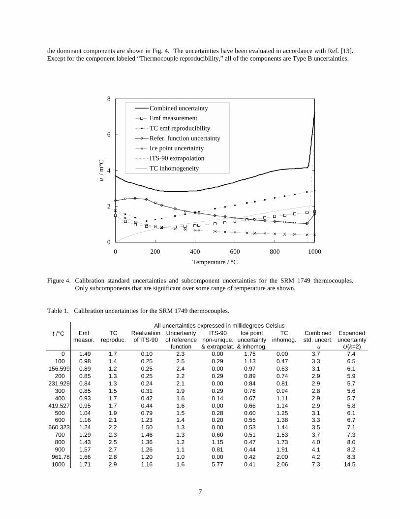
Table 1 lists the calibration uncertainty of the SRM 1749 thermocouples at fixed point temperatures and a number ofadditional temperatures. Each of the subcomponents of uncertainty mentioned in Table 1 are discussed below, and

7

the dominant components are shown in Fig. 4. The uncertainties have been evaluated in accordance with Ref. [13].Except for the component labeled “Thermocouple reproducibility,” all of the components are Type B uncertainties.

Figure 4. Calibration standard uncertainties and subcomponent uncertainties for the SRM 1749 thermocouples.Only subcomponents that are significant over some range of temperature are shown.

Table 1. Calibration uncertainties for the SRM 1749 thermocouples.

All uncertainties expressed in millidegrees Celsiust /°C Emf

measur.TC

reproduc.Realizationof ITS-90

Uncertaintyof reference

function

ITS-90non-unique.& extrapolat.

Ice pointuncertainty& inhomog.

TCinhomog.

Combinedstd. uncert.

u

Expandeduncertainty

U(k=2)0 1.49 1.7 0.10 2.3 0.00 1.75 0.00 3.7 7.4

100 0.98 1.4 0.25 2.5 0.29 1.13 0.47 3.3 6.5156.599 0.89 1.2 0.25 2.4 0.00 0.97 0.63 3.1 6.1

200 0.85 1.3 0.25 2.2 0.29 0.89 0.74 2.9 5.9231.929 0.84 1.3 0.24 2.1 0.00 0.84 0.81 2.9 5.7

300 0.85 1.5 0.31 1.9 0.29 0.76 0.94 2.8 5.6400 0.93 1.7 0.42 1.6 0.14 0.67 1.11 2.9 5.7

419.527 0.95 1.7 0.44 1.6 0.00 0.66 1.14 2.9 5.8500 1.04 1.9 0.79 1.5 0.28 0.60 1.25 3.1 6.1600 1.16 2.1 1.23 1.4 0.20 0.55 1.38 3.3 6.7

660.323 1.24 2.2 1.50 1.3 0.00 0.53 1.44 3.5 7.1700 1.29 2.3 1.46 1.3 0.60 0.51 1.53 3.7 7.3800 1.43 2.5 1.36 1.2 1.15 0.47 1.73 4.0 8.0900 1.57 2.7 1.26 1.1 0.81 0.44 1.91 4.1 8.2

961.78 1.66 2.8 1.20 1.0 0.00 0.42 2.00 4.2 8.31000 1.71 2.9 1.16 1.6 5.77 0.41 2.06 7.3 14.5

0

2

4

6

8

0 200 400 600 800 1000Temperature / °C

u /

m°C

Combined uncertaintyEmf measurementTC emf reproducibilityRefer. function uncertaintyIce point uncertaintyITS-90 extrapolationTC inhomogeneity

8

5.1 Thermocouple reproducibilityThe reproducibility of emf measurements in fixed-point cells of a set of Au/Pt thermocouples, with constructionvery similar to the SRM 1749 thermocouples, was determined in the original work on the reference function forAu/Pt thermocouples [7]. This reproducibility was taken as the Type A uncertainty for the calibration of the SRM1749 thermocouples. When expressed as an equivalent temperature uncertainty, the Type A uncertainty could berepresented by the expression uA = 0.201×10−5(t /°C) + 0.86 m°C for the fixed points indium, tin, cadmium, zinc,aluminum, and silver. The Type A uncertainty for the ice point was determined from repeat measurements onseveral thermocouples in the SRM 1749 lot. The value found was uA(ice) = 1.74 m°C. In Table 1, this uncertaintyis termed the “Reproducibility of Au/Pt TCs”, but more accurately can be considered to include also effects of thereproducibility of the emf measurements, the reproducibility of the reference junction bath, the thermoelectricinstability of the thermocouples over the course of the calibration measurements, and the reproducibility of thefixed-point realizations.

5.2 Emf measurement uncertaintiesUncertainties of the emf measurements not covered in the Type A uncertainty were determined by independentmeasurements of the variation of the thermal emfs from the scanner relays and wiring, measurement of the voltmeternon-linearity, measurements of the gain stability of the multimeter over extended periods of time, and byintercomparison of the multimeter with other multimeters of the same and different manufacturer.

Figures 5 and 6 display typical results for the voltmeter nonlinearity, as measured on a Resistance Bridge Calibrator(RBC) [14]. The RBC is similar to a Hamon network of resistors [15], but is configured in such a way as to allowup to 35 independent resistance values to be obtained from serial and parallel combinations of only four resistors.Because of this large redundancy of resistance values, the four base resistance values may be obtained from a least-squares fit of the values to the data. The four resistors need not be calibrated independently.

Figure 5. Tests of the non-linearity of a digital voltmeter at low voltage values. The four symbols represent fourseparate runs on different days.

−30

−20

−10

0

10

20

30

0 3 6 9 12 15Voltage / mV

Dev

iatio

n fr

om li

near

ity /

nV

(offset) (total non-linearity)u u

9

Figure 6. Test of the non-linearity of a digital voltmeter on the range with full scale voltage of 1.2 V.

Although the RBC is designed as an instrument for AC measurements or for DC measurements with frequentcurrent reversals, it can be used with DC measurement systems provided that the thermal emfs in the RBC and itsassociated wiring are dramatically reduced. To reduce the thermal emfs of the wiring, it is necessary to use leadwires that are very similar in thermoelectric properties to the other lead wires and to the internal wiring of the digitalvoltmeter. This is accomplished by using twisted pairs of untinned copper wire instead of coaxial cable for thewiring. Thermal emfs inside the RBC are reduced dramatically by reducing the temperature gradients in the vicinityof the RBC. This is accomplished by thermally isolating the RBC inside concentric boxes of polystyrene foam,aluminum 0.8 cm thick, and polystyrene foam. The rms thermal emfs of the RBC connections when insulated inthis fashion were less than 3.5 nV. In typical operation, the RBC is used to measure the non-linearity, offset, andgain error (these terms are defined in Section 10) of instruments that measure resistance ratios, the instrumentreading being a measurement of the ratio of a test resistance to that of a reference resistance. For the purpose ofmeasuring the non-linearity and offset of a voltmeter, a fixed current was passed through the RBC and an external,temperature-controlled reference resistor, both of which were connected in series. Resistance ratios wereconstructed by dividing the voltage measured across the RBC by the voltage measured across the reference resistor.The readings were corrected for the voltmeter zero readings either by averaging measurements with two directionsof current, or by subtracting voltmeter readings made with zero current from the readings with current. As aconsequence of using an external reference resistor that was not independently calibrated relative to the RBC baseresistors, it was not possible to determine the voltmeter gain error with the RBC. The rms deviation of the readingsfrom the simple model used to fit the RBC data is expected to equal the sum of the measurement noise and thevoltmeter non-linearity, added in quadrature. Sources of measurement noise include both short-term fluctuations inthe current source and the inherent noise of the digital voltmeter. At low voltages, the inherent voltmeter noisedominates the measurement noise, and each data point requires approximately seven minutes of signal averaging. Bysubtracting the independently-measured voltage noise from the rms deviation, we obtain an estimate of the non-linearity. The results of the RBC on the 100 mV voltmeter range indicate that the emf measuring system has acombined offset error (δ in Section 10) and non-linearity of only 0.0085 µV at the one standard deviation level,which we round to 0.01 µV. On the 1 V range, the offset is negligible, and the non-linearity is of the samemagnitude as the measurement noise. Because we did not perform multiple runs on multiple higher voltage ranges,we chose to conservatively estimate the non-linearity on the higher ranges as the rms deviation from ideal behavior,without any subtraction of measurement noise. Previous measurements of the same model of voltmeter against aJosephson junction array gave similar results [16]. As shown in Fig. 6, the non-linearity is 2×10−7 of the reading, forreadings of 16 % of nominal full scale and above.

We measured the gain error on the 10 V range directly by measuring a calibrated 10 V solid-state voltage reference.On the 100 mV range, which is the only range used for Au/Pt thermocouple measurements, it is possible todetermine the gain error of the voltmeter by two simple methods. One straightforward method is to construct a

−6.Ε−07

−4.Ε−07

−2.Ε−07

0.Ε+00

2.Ε−07

4.Ε−07

6.Ε−07

0 0.2 0.4 0.6 0.8 1 1.2 1.4Voltage / V

Frac

tiona

l non

-line

arity

Measurement noise, 1 std. dev.

10

calculable 100 mV or 10 mV voltage source, based on a 1:1000 or 1:10,000 voltage divider constructed from twoindependently-calibrated four-terminal resistors that are connected in series. Passing a suitable DC current throughthe resistors produces voltages of nominally 10 V and 100 mV or 10 mV, whose exact ratio can be calculated fromthe resistor calibrations. A second method for determining the scale error relies on the high degree of linearity of thevoltmeter, as shown in Fig. 5 and 6. If the voltmeter was perfectly linear, then the scale error of one range relativeto another range can be determined by measuring the ratio of two determinations of the same voltage, on the twoscales. For example, a 100 mV voltage can be read on both the 1 V scale and the 100 mV scale. In practice, anadditional uncertainty must be added to account for the voltmeter non-linearity. We used this second method.

The voltmeter gain error (α in Section 10) is dominated by changes in the gain sensitivity of the voltmeter as thevoltmeter temperature varies during the course of the day. Figure 7 shows variations in the ratio of the voltmeterreadout to the true voltage, for a voltage of 100 mV, and as a function of the voltmeter internal temperature.

When these effects are combined, the Type B standard uncertainty for the combined scanner and digital multimetersystem can be expressed as u/µV = 2.5×10-6(E/µV) + 0.01, where E is the thermocouple emf. A summary of thesubcomponents of this expression is listed in Table 2.

Figure 7. Fractional deviation of measured voltage at 100 mV from value of voltage expected by scaling down froma 10 V reference, as a function of the temperature change from time of autocalibration.

Table 2. Subcomponents of the gain uncertainty for the digital voltmeter, expressed as fractional standarduncertainty in E.

Subcomponent Fractional standarduncertainty in E

Temperature change in voltmeter 1.2×10−6

Voltmeter non-linearity 1.2×10−6

Voltmeter calibration drift 1.0×10−6

10 V dc voltage reference 1.5×10−6

Combined gain uncertainty 2.5×10−6

−1.5Ε−06

−1.0Ε−06

−5.0Ε−07

0.0Ε+00

5.0Ε−07

1.0Ε−06

1.5Ε−06

−0.8 −0.4 0.0 0.4 0.8[T (Measurement) − T (Calibration)] / °C

Frac

tiona

l dev

iatio

n

Run 1Run 2Run 3Run 4

Slope (−1.35E−6)/K

11

5.3 Realization of the ITS-90For measurements at each fixed point, a Type B uncertainty was included to account for deviations of our cells froman ideal fixed point of a pure material. These deviations were determined by measurements of freezing plateauswith an SPRT or a high temperature SPRT, by comparison with the reference standard cells maintained by thePlatinum Resistance Thermometry Laboratory at NIST, and by estimation of uncertainty from known impurities. Inthe data analysis, corrections were made to the fixed-point cell temperature for the hydrostatic head and for thetemperature difference between the cells used for this study and the reference standard cells maintained in thePlatinum Resistance Thermometry Laboratory.

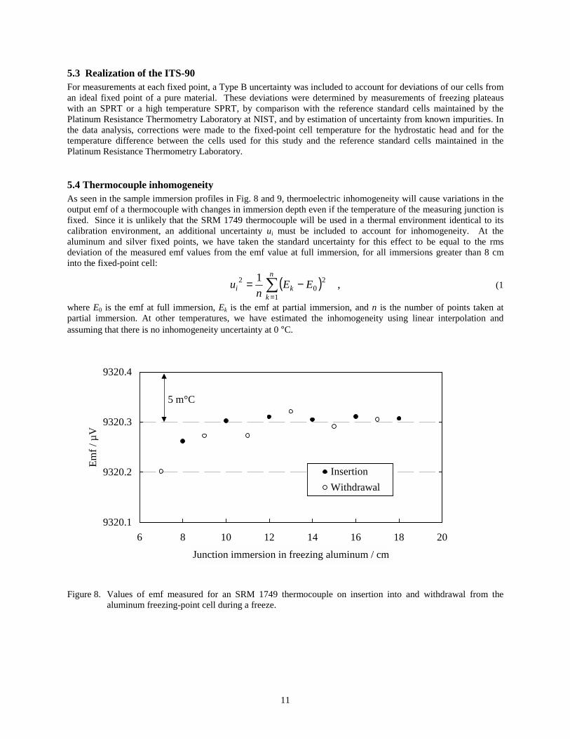
5.4 Thermocouple inhomogeneityAs seen in the sample immersion profiles in Fig. 8 and 9, thermoelectric inhomogeneity will cause variations in theoutput emf of a thermocouple with changes in immersion depth even if the temperature of the measuring junction isfixed. Since it is unlikely that the SRM 1749 thermocouple will be used in a thermal environment identical to itscalibration environment, an additional uncertainty ui must be included to account for inhomogeneity. At thealuminum and silver fixed points, we have taken the standard uncertainty for this effect to be equal to the rmsdeviation of the measured emf values from the emf value at full immersion, for all immersions greater than 8 cminto the fixed-point cell:

( ) ,1

1

20

2

=−=

n

kki EE

nu (1

where E0 is the emf at full immersion, Ek is the emf at partial immersion, and n is the number of points taken atpartial immersion. At other temperatures, we have estimated the inhomogeneity using linear interpolation andassuming that there is no inhomogeneity uncertainty at 0 °C.

Figure 8. Values of emf measured for an SRM 1749 thermocouple on insertion into and withdrawal from thealuminum freezing-point cell during a freeze.

9320.1

9320.2

9320.3

9320.4

6 8 10 12 14 16 18 20

Junction immersion in freezing aluminum / cm

Emf /

µV

InsertionWithdrawal

5 m°C

12

Figure 9. Values of emf measured for an SRM 1749 thermocouple on insertion into and withdrawal from the silverfreezing-point cell during a freeze.

The stated inhomogeneity uncertainty, ui, and combined expanded uncertainty, U, apply when the SRM 1749thermocouple is used in apparatus where the immersion distance, L, from the coil of the measuring junction to thepoint at the throat of the furnace where there is a maximal thermal gradient is in the range 36 cm to 44 cm. For thetwo NIST furnaces used for all of the fixed-point measurements, this distance ranged from 38 cm to 44 cm. If theSRM 1749 thermocouple is used at an immersion significantly shorter than 36 cm from the point of maximumthermal gradient to the measuring junction, it is recommended that the uncertainty be recalculated according to thefollowing formulas:

( ) ,cm 8cm 36ii i, L uuu L −+= (2

( ) ,2/12

,i2

i2

LL uuUU +−= (3where ui,L is the standard uncertainty subcomponent for the thermocouple inhomogeneity at an immersion depth of Land UL is the combined expanded uncertainty at the specified immersion depth.

5.5 Uncertainty of the reference functionIn the calibration procedure, the true emf-temperature relation of the thermocouple is modeled as the referencefunction for Au/Pt thermocouples plus a quadratic function. This model is an approximation, with an associateduncertainty. Attempts to fit a cubic or higher order polynomial to the emf deviation data did not result in astatistically superior fit. If there are errors in the reference function that can be modeled with a quadratic function,such errors have no net effect on the uncertainty of the combined model of reference function plus quadraticfunction. This implies that the appropriate uncertainty is the uncertainty of the reference function over temperatureranges characteristic of the difference in temperature values of adjacent fixed points, which ranges from 75 °C to301 °C. Because the number of degrees of freedom in the determination of the Au/Pt reference function was veryhigh [7], the statistical uncertainty is generally small except at 1000 °C, and a good measure of the short-rangeuncertainty of the reference function is the systematic discrepancy between data obtained by fixed-pointmeasurements and data obtained by comparison with an SPRT in the original determination of the referencefunction. This uncertainty for the Au/Pt thermocouple reference function is 0.04 µV at 1000 °C, 0.026 µV from thesilver freezing point at 962 °C to the indium point at 157 °C, and decreases to approximately 0.014 µV fortemperatures near 10 °C.

16120.1

16120.2

16120.3

16120.4

6 8 10 12 14 16 18 20

Junction immersion in freezing silver / cm

Emf /

µV

InsertionWithdrawal

4 m°C

13

5.6 Uncertainty of the ice pointAn ice point as prepared according to the methods described in Section 9 has a standard reproducibility of 1 m°C[17]. No uncertainty term has been added to account for the reproducibility of the ice point, since the Type Auncertainty for the reproducibility of the thermocouples emf at the various fixed points already incorporates anyeffects of variations in the ice points. However, we have added an uncertainty to account for any systematic errorsin the NIST ice points caused by impurities in the distilled water used for the preparation of the ice and ice baths.Measurements of ice baths prepared from the same distilled water supply as used in the SRM 1749 calibrationrevealed a –0.6 m°C depression below the nominal value of 0 °C. The data has been corrected for this 0.6 m°Coffset, and a square uncertainty distribution of ±1 m°C has been included for systematic variations in the ice pointtemperature.

Because of slight variations in the physical or chemical characteristics of the wires inside the reference-junctionprobe, the emf generated by the SRM 1749 thermocouples between room temperature and the reference junctionswill vary slightly depending on the depth of immersion of the probe into the ice, even for immersion depths deepenough to ensure that the reference junctions are maintained at 0 °C. An uncertainty for this effect of referenceprobe inhomogeneity has been included to account for a variation of up to 1 cm in ice level or thickness of thereference bath cover in the user’s laboratory compared to those at NIST. It is important to carefully adhere to theprocedures of Section 9 to minimize these inhomogeneity effects. If different procedures are used, it is the user’sresponsibility to determine the effect on the thermocouple emf of using an ice point of different preparation ordesign. Preferably, this effect is determined by actual measurement of the emf differences obtained when themeasuring junction is maintained at a fixed temperature and the bath used for the reference junction is alternatedbetween the user’s design and a bath prepared following Section 9.

5.7 Summary of uncertaintiesAs seen in Table 1 and Fig. 4, no single uncertainty component dominates the combined uncertainty over the fulltemperature range. At low temperatures, the uncertainty of the reference function is dominant. Above 962 °C, thereference function is based on an extrapolation of the ITS-90, which is not well known, and this becomes thedominant uncertainty. For intermediate temperatures, the thermocouple reproducibility, the uncertainty of the emfmeasurements, and the thermocouple inhomogeneity are all significant.

6. Properties of thermocouples prepared for SRM 1749

The emf deviation, defined as the difference between the measured emf of a particular thermocouple and thereference thermocouple, is a convenient means of comparing the emf-temperature relation of a thermocouple to thereference function. Figure 10 shows the average, maximum, and minimum emf deviation for the lot of SRM 1749thermocouples. The maximum deviation from the reference function for all 18 thermocouples in the lot is 0.22 µVat the aluminum freezing point, equivalent to 11 m°C. The maximum spread in the emf values at any of the fixedpoints is 0.21 µV at the silver freezing point, equivalent to 8.5 m°C, which is approximately a factor of 10 smallerthan we observe with platinum-rhodium alloy thermocouples fabricated from the same lots of wire. The smallspread in the emf values is an indication that the gold and platinum wires used to fabricate the thermocouples werechemically homogeneous, and that the annealing procedures used in the fabrication process were highlyreproducible and uniform.

The scatter at each fixed-point temperature shown in Fig. 10 is not random. Correlation plots of the emf deviation atone fixed-point temperature versus the emf deviation at another fixed-point temperature show a high degree ofcorrelation for the emf measurements at the lower-temperature fixed points. This can be seen in the representativeplots in Fig. 11 and 12. At the higher temperatures, there are correlations in the emf readings, but the correlation isrelatively weak compared to the thermocouple reproducibility, as seen in Fig. 13. This result confirms that there arestatistically significant differences in the emf-temperature relationships of the 18 thermocouples in the lot at lowertemperatures and that individual calibration gives a smaller combined uncertainty than using an average calibrationfor the lot.

14

Figure 10. Differences between the measured emf values for the SRM 1749 thermocouples and the referencefunction for Au/Pt thermocouples. Solid circles indicate the average values for all thermocouples, theopen circles indicate maximum and minimum values, and the error bars indicate one standard deviationvariations in the emf values.

Figure 11. Correlation of emf values at the aluminum point, E(Al), with emf values at the silver point, E(Ag). Solidcircles are for the SRM 1749 thermocouples. Open circles are from additional thermocouples fabricatedfrom the same lots of wire as the SRM 1749 thermocouples.

−0.12

−0.08

−0.04

0.00

0.04

0.08

0.12

−0.15 −0.10 −0.05 0.00 0.05 0.10 0.15

Fixed-point reproducibility,1 std. deviation

[E(Ag) − E(Ag)] / µV

[E(A

l) − E

(Al)

] / µ

V

−0.3

−0.2

−0.1

0.0

0.1

0.2

0 200 400 600 800 1000Temperature / °C

Emf d

evia

tion

/ µV

Ice

In

SnZn Al

Ag

−10 m°C

10 m°C

15

Figure 12. Correlation of emf values at the ice point, E(Ice), with emf values at the indium point, E(In). Solid circlesare for the SRM 1749 thermocouples. Open circles are from additional thermocouples fabricated fromthe same lots of wire as the SRM 1749 thermocouples.

0

1

2

3

4

0 200 400 600 800 1000Temperature / °C

Lot v

aria

tion

/ Rep

rodu

cibi

lity

TCs selected for SRM 1749Full set of 21 TCs fabricated

Ice

In SnZn

Al Ag

Figure 13. Ratio of the standard deviation of emf values in the lot of SRM 1749 thermocouples at each fixed point tothe standard deviation for the reproducibility of Au/Pt thermocouples with extended thermal cycling.

Because the Seebeck coefficient is quite small near 0 °C, over a factor of four smaller than at 1000 °C, the emfdeviations of the SRM 1749 thermocouples at the ice point are equivalent to relatively large temperature deviations.The average deviation in units of temperature is −11 m°C at 0 °C. This result confirms the necessity of includingthe ice point as a calibration point.

Figures 8 and 9 show representative immersion profiles at the aluminum and silver fixed-point cells. These resultsare very typical of high-quality Au/Pt thermocouples, showing little variation in emf values beyond an immersion of8 cm of the measuring junction below the surface of the freezing metal. At the silver freezing point, there isnoticeable hysteresis between measurements taken on insertion of the thermocouple into the cell, compared tomeasurements taken on withdrawal. This is most probably a result of reversible metallurgical changes, such as a

−0.06

−0.04

−0.02

0.00

0.02

0.04

−0.04 −0.02 0.00 0.02 0.04

Fixed-point reproducibility,1 std. deviation

[E(In) − E(In)] / µV

[E(Ic

e) −

E(I

ce)

] / µ

V

16

change in the number of lattice vacancies in the thermoelements, or possibly changes in the oxidation state of theplatinum. When annealed at 450 °C for 10 h, the metallurgical state of the thermoelements attains thermalequilibrium. On subsequent use at higher temperatures, the sections of the thermoelements exposed to significantlyhigher temperature will have an increased number of lattice vacancies. As the thermocouple is first inserted into andthen withdrawn from the furnace, the thermoelements will acquire a nonuniform distribution of lattice vacanciesalong the thermoelement length.

Measurements were also made of the sensitivity of the thermocouple emf to immersion of the reference-junctionprobe. These measurements showed that immersion of at least 20 cm into the ice/water mixture was sufficient toassure thermal equilibrium of the reference junctions with the ice/water mixture. On insertion of a reference-junction probe from room temperature into an ice bath, it is necessary to wait ten minutes for the reference junctionsinside the probe to reach a steady state temperature, within the uncertainty of the calibration.

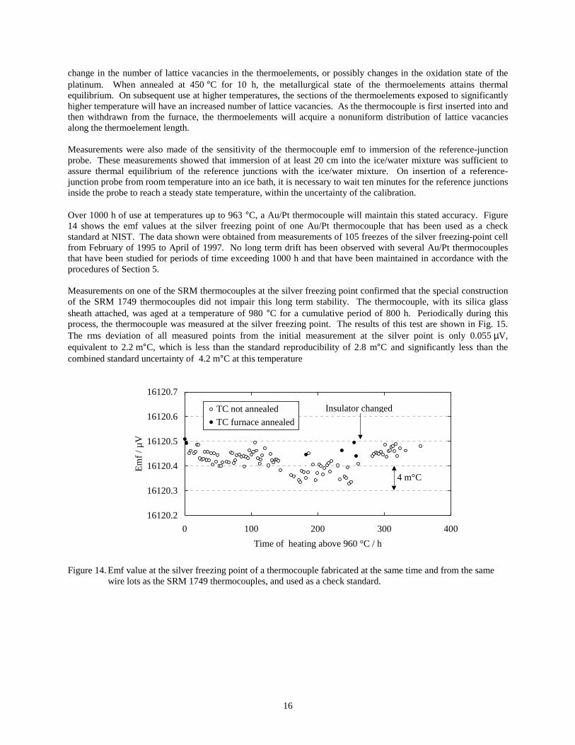
Over 1000 h of use at temperatures up to 963 °C, a Au/Pt thermocouple will maintain this stated accuracy. Figure14 shows the emf values at the silver freezing point of one Au/Pt thermocouple that has been used as a checkstandard at NIST. The data shown were obtained from measurements of 105 freezes of the silver freezing-point cellfrom February of 1995 to April of 1997. No long term drift has been observed with several Au/Pt thermocouplesthat have been studied for periods of time exceeding 1000 h and that have been maintained in accordance with theprocedures of Section 5.

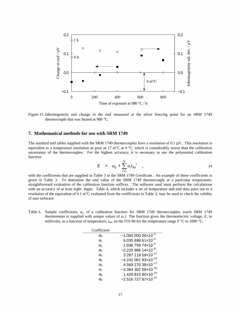
Measurements on one of the SRM thermocouples at the silver freezing point confirmed that the special constructionof the SRM 1749 thermocouples did not impair this long term stability. The thermocouple, with its silica glasssheath attached, was aged at a temperature of 980 °C for a cumulative period of 800 h. Periodically during thisprocess, the thermocouple was measured at the silver freezing point. The results of this test are shown in Fig. 15.The rms deviation of all measured points from the initial measurement at the silver point is only 0.055 µV,equivalent to 2.2 m°C, which is less than the standard reproducibility of 2.8 m°C and significantly less than thecombined standard uncertainty of 4.2 m°C at this temperature

Figure 14. Emf value at the silver freezing point of a thermocouple fabricated at the same time and from the samewire lots as the SRM 1749 thermocouples, and used as a check standard.

16120.2

16120.3

16120.4

16120.5

16120.6

16120.7

0 100 200 300 400Time of heating above 960 °C / h

Emf /

µV

TC not annealedTC furnace annealed

4 m°C

Insulator changed

17

Figure 15. Inhomogeneity and change in the emf measured at the silver freezing point for an SRM 1749thermocouple that was heated at 980 °C.

7. Mathematical methods for use with SRM 1749

The standard emf tables supplied with the SRM 1749 thermocouples have a resolution of 0.1 µV. This resolution isequivalent to a temperature resolution as poor as 17 m°C at 0 °C, which is considerably worse than the calibrationuncertainty of the thermocouples. For the highest accuracy, it is necessary to use the polynomial calibrationfunction

,1

900 =

+=N

i

iitaaE (4

with the coefficients that are supplied in Table 3 in the SRM 1749 Certificate. An example of these coefficients isgiven in Table 3. To determine the emf value of the SRM 1749 thermocouple at a particular temperature,straightforward evaluation of the calibration function suffices. The software used must perform the calculationswith an accuracy of at least eight digits. Table 4, which includes a set of temperature and emf data pairs out to aresolution of the equivalent of 0.1 m°C evaluated from the coefficients in Table 3, may be used to check the validityof user software.

Table 3. Sample coefficients, ai, of a calibration function for SRM 1749 thermocouples. (each SRM 1749thermometer is supplied with unique values of ai.) The function gives the thermoelectric voltage, E, inmillivolts, as a function of temperature, t90, on the ITS-90 for the temperature range 0 °C to 1000 °C.

Coefficienta0 −1.050 000 00×10−4

a1 6.035 698 61×10−3

a2 1.936 759 74×10−5

a3 −2.229 986 14×10−8

a4 3.287 118 59×10−11

a5 −4.242 061 93×10−14

a6 4.569 270 38×10−17

a7 −3.394 302 59×10−20

a8 1.429 815 90×10−23

a9 −2.516 727 87×10−27

1 h

0 h

−0.1

0.0

0.1

0.2

0 200 400 600 800Time of exposure at 980 °C / h

Cha

nge

in e

mf /

µV

−0.1

0.0

0.1

0.2

Inho

mog

enei

ty st

d. d

ev. /

µV

4 m°C

18

Table 4. Temperature-emf data pairs evaluated from the coefficients in Table 3, to a resolution of the equivalent of0.1 m°C. These data pairs may be used to check the validity of user software.

t90 / °C E/mV0 −0.000 105 0

100 0.777 746 3200 1.844 884300 3.141 542400 4.633 170500 6.300 671600 8.134 800700 10.131 941800 12.290 580900 14.609 001

1000 17.085 005

Table 5. Coefficients ci of an approximate inverse function for Au/Pt thermocouples. This function givestemperature, t90, in degrees Celsius as a function of the thermoelectric voltage, E, in millivolts in thespecified temperature and voltage range. The error of this inverse function is ±1 °C. See Eq. 5. Note thatthe error of this inverse function is much larger than the error of the inverse function in Ref. [18], which issomewhat more mathematically complex. The function below should be used only in conjunction withthe method of section 7.

Coefficientc0 0.000 000c1 1.545 738×102

c2 −4.219 267×101

c3 1.351 401×101

c4 −2.888 146c5 3.931 653×10−1

c6 −3.366 290×10−2

c7 1.751 092×10−3

c8 −5.047 341×10−5

c9 6.176 037×10−7

To determine the temperature value of the SRM 1749 thermocouple at a measured emf value requires a morecomplex method. Because there is no exact inversion of the polynomial calibration function, a numerical inversiontechnique must be used. The steps of this procedure are as follows:

1. Evaluate the approximate inverse temperature tapp, using the inverse function

,1

m0app =

+=N

i

ii Ecct (5

where the coefficients ci are listed in Table 5 and Em is the measured value of emf in units of millivolts. (Theapproximate inverse equation given in Ref. [18] may also be used. This alternate function gives a somewhatmore accurate initial value for tapp, but it is only the tolerance specified in step 5, and not the choice ofapproximate inverse function, that determines the accuracy of the final value of t.)

2. Define the function G(t) = Em – Ecal(t), where Ecal(t) is the SRM 1749 calibration function given in Table 3 ofthe Certificate.

3. The derivative of G(t) is given as

( ) .1

1

=

−−=′N

i

iitiatG (6

19

4. Use the iterative technique termed Newton’s method to find the value of t that will give G(t) = 0. This valueof t is the desired temperature value corresponding to the measured emf value. For each iteration ofNewton’s method, an improved temperature value, t1, is determined from a starting value of temperature, t0,using the equation:

( ) ( ) .0001 tGtGtt ′−= (7For the first iteration, t0 = tapp. For later iterations, the value of t0 is taken as the value of t1 determined in theprevious step.

5. Repeat iterations of Newton’s method until the change |t0 – t1| is less than a tolerance set by the user.

In practice, only one or two iterations will be necessary, since all of the SRM 1749 thermocouples are a very closematch to the reference function. Again, for checking user software, Tables 3 and 4 are useful.

8. Maintenance of the thermocouple

Pure element thermocouples are fairly rugged devices, capable of withstanding repeated thermal cycling and smallmechanical shocks. However, three maintenance procedures are necessary to ensure that there is no degradation inaccuracy.

First, the platinum expansion coil at the measuring junction should be inspected periodically. At room temperature,both thermoelements should extend from the alumina tube by the same amount as when the thermocouple was firstmanufactured. If the protrusion of one of the thermoelements increases by more than about 1 mm after a period ofheating to elevated temperatures and then cooling to room temperature, the thermoelement may have seized slightlyin the bore of the alumina tube and may have been mechanically strained.

Second, pure element thermocouples should be given a periodic maintenance anneal especially if they are removedquickly from high temperature environments or if they are used in different thermal environments. The procedurefor Au/Pt thermocouples is to furnace anneal the thermocouple at 450 °C overnight at the fullest possible immersionof the thermocouple into the furnace. This procedure reduces the number of lattice vacancies quenched into thethermoelements when the thermocouple is removed rapidly from a high-temperature environment. At NIST, thefurnace used for furnace annealing is a three zone, horizontal tube furnace. During a heat treatment, the temperaturealong the portion of the thermocouple extending from its measuring junction to approximately 62 cm from thejunction was uniform within 2 °C.

Third, the copper leads of the SRM 1749 thermocouple are not plated, and will become oxidized with time.Although the use of a junction box similar to the one described in Section 10 will minimize the thermal gradientsnear the terminals, it is still recommended that the copper oxide be removed occasionally by pulling the short,exposed sections of bare copper lead wire gently through a folded abrasive pad. With extensive use, these copperwires may become work-hardened and fragile. In this event, the user may cut off the short affected length of copperwire and strip off a short section of wire insulation without affecting the calibration of the thermocouple.

9. Preparation of an ice bath for the reference junctions

The low uncertainty of the SRM 1749 thermocouples requires a carefully prepared ice bath to maintain thetemperature of the reference-junction probe at 0 °C. A properly prepared ice bath will have an expanded uncertaintyof 2 m°C.

The ice for the ice bath should be finely-crushed or shaved ice that has been prepared from distilled water. The iceshould be saturated with distilled water, and then packed gently into an insulating Dewar flask, such that ice fullyfills the volume of the flask with no large voids. At NIST, a cylindrical flask (7 cm inner diameter and 30 cm deep)having a polyethylene-foam cover, 2.5 cm thick, is used. Other flask geometries are allowable, provided the flask isat least 6 cm inner diameter and 30 cm deep, and the thickness of the cover is in the range 1.5 cm to 3 cm. The levelof the ice-water mixture should be within 5 mm of the bottom surface of the cover. The cover should have a hole ofapproximate diameter 6.3 mm in the center, to allow insertion of the reference-junction probe of the SRM 1749 into

20

the ice point. The reference-junction probe should be inserted until the stop on the probe is butted against the flaskcover. Since the ice in the Dewar flask will tend to float as the ice melts, a rubber band should be used to secure thecover onto the flask.

The use of electronic ice-point compensators, extension wires, and automated ice points cooled with thermoelectricmodules is not recommended unless a careful analysis of the additional uncertainties is performed. These devices,in general, contribute additional errors to the measurement that are large relative to the calibration uncertainty of theSRM 1749.

It is possible to use a triple point of water (TPW) cell to maintain the reference junctions at a temperature of 0.01 °C.If this is done, a quantity of 0.056 µV should be added to the measured emf to compensate for the referencetemperature differing from the nominal 0 °C. The enclosure used to maintain the TPW cell should be configured sothat the thermal profile along the reference-junction probe of the SRM 1749 is similar to the profile that the probewould be exposed to in a ice bath as described above.

10. Emf measurements

The calibration uncertainty of the SRM 1749 thermocouples, when expressed in units of voltage, ranges from anexpanded uncertainty of 0.04 µV at a thermocouple signal of 0 µV (0 °C) to 0.37 µV at a thermocouple signal of17,085 µV (1000 °C). In comparison, many voltmeters have expanded uncertainties significantly greater than this.In order to achieve the inherent accuracies possible with the SRM 1749 thermocouple, it is necessary to select theequipment for the voltage measurements carefully and to take the measurements using proper procedures. Thissection describes considerations for equipment selection and describes the methods used at NIST to measurevoltage.

Although it is possible to connect the SRM 1749 thermocouple directly to a digital voltmeter, lower measurementuncertainties and greater convenience are possible by connecting the digital voltmeter to a scanner, which is aninstrument that allows sequential connection of a voltmeter (or other instrument) to any one of a number of voltagesources. A single set of terminals to be used for reading one voltage source consists of a positive-polarity terminal,a negative-polarity terminal, and possibly a guard terminal, and is commonly termed a “channel” on the scanner.Because the terminals for each channel are often not conveniently placed for attaching leads of the thermocouple, itis desirable to extend the terminal connections of the scanner to a specially-constructed junction box. Consequentlythere are three pieces of equipment needed for high accuracy voltage measurements: a digital voltmeter, a scanner,and a junction box. Each of these items will be considered below, and then the data acquisition procedures to beused for the combined system will be described.

10.1 Digital voltmetersManufacturers typically state the specifications for DC voltage measurements with a digital voltmeter as a fractionof the voltage E that is measured, plus a fraction of the range. For example, on a 100 mV range, the specificationsmay be quoted as 4Η10−6 of reading plus 3Η10−6 of range, which is mathematically expressed as a tolerance a=(4Η10−6E + 0.3 µV). If the user does no further characterization of the voltmeter, then the standard uncertaintycontributed by the voltmeter may be estimated by assuming that the manufacturer’s tolerance sets bounds ∀ a for arectangular distribution of measurement errors. The standard uncertainty of such a distribution is a/√3, or for theexample above, u(E) = (4Η10−6E + 0.3 µV)/√3.

In practice, we have found that it is possible with proper measurement techniques to greatly reduce the componentof u(E) that is independent of E. To achieve a smaller value of u(E) it is necessary to understand the various effectsthat can cause voltmeter measurement uncertainties. The sources of voltage measurement errors include thefollowing effects:

1. Gain error of the voltmeter, resulting in R = (1 + α)E, where R is the reading of the voltmeter and α =constant. Although α is independent of E, it will in general vary with the temperature of the voltmeter andmay change over periods of time from several days to several months.

21

2. Offset error of the voltmeter, resulting in R = E + δ. Typical sources of δ are differences in the thermal emfsinside the voltmeter relative to the thermal emfs that existed when the voltmeter was calibrated, and possiblyother noise contributions that vary at such a low frequency that signal averaging is ineffective. The value of δvaries over time scales ranging from several minutes to several months.

3. Nonlinearity of the voltmeter, resulting in higher order terms in the R(E) relation than can be modeled with asimple linear relation. In most modern voltmeters, the non-linearity is of the same order as the magnitude ofthe least significant digit.

Of these three components, only the offset error is amenable to reduction by the user. Non-linearity is difficult tomeasure and tends to be a small effect in any case. The gain error in general is different for each measurement rangeand may vary substantially as the internal temperature of the voltmeter varies. One could correct for gain error bymeasurements of a reference voltage every hour or so on the same range as the thermocouple measurements, but it isdifficult to build or obtain a reference voltage of sufficient accuracy at the low voltages generated by thermocouples.

Fortunately, the offset error is often a large contribution to the overall uncertainty, and demonstrated reduction in theoffset error can justify a reduction in u(E). A procedure that is effective in both reducing the offset error of thevoltmeter and in correcting for thermal emfs contributed by the scanner is described in the Sections 10.2 and 10.4. Inselecting a voltmeter for use with the SRM 1749, there is no perfect choice. So called “nanovoltmeters” have lowoffset errors but relatively large gain errors. These units are ideal when the manufacturer’s specifications for theterm in the DC voltage accuracy proportional to E is acceptably low. Other voltmeters without input stagesoptimized for low voltages, but with a high number of significant digits in the readout, typically have larger offseterrors and greater noise, but substantially smaller gain errors than nanovoltmeters. With careful measurementtechniques and with sufficient signal averaging to reduce the measurement noise, this type of meter has given themost accurate results at NIST.

10.2 ScannersAt NIST, we have had success with a variety of scanners that have been optimized for low-level DC voltagemeasurements. Some scanners have been designed with extremely low thermal emfs (less than 50 nV), and theseare highly appropriate for use with the SRM 1749 thermocouple. Surprisingly, scanners with specifications that aresignificantly less stringent will serve well provided that the scanner is appropriately selected and that the dataacquisition procedure described below is followed. As a general rule, avoid scanners that route analog signals viamultipin connectors, which can be a significant source of extraneous thermal emf. As an example of a connectortype that should be avoided for measurements of the highest accuracy, some scanners require that the signal leads beterminated at a multipin connector, which then is plugged into a mating connector on a circuit board of the scanner.The signal path from the thermocouple should pass through only screw connectors, copper wires or circuit boardtraces, and the relays. Multipin connectors that provide power or that route digital control signals are acceptable. Ifthe scanner uses electromechanical relays that are continuously energized while a particular channel is being read,the heat from the relay coil may cause significant changes in the thermal emfs. This effect can be minimized by a)energizing each relay for no more than 1 minute at a time, b) using each relay at a duty cycle of no more than 20%,and c) setting the scanner to a specially-designated “hold” channel when data is not being acquired. To achieve thelow duty cycle while still utilizing all available measurement time, it is convenient to route the thermocouple signalto several pairs of terminals by using bare copper wires between terminals on the junction box.

Even with the above precautions, we have found that most commercial scanners still have extraneous thermal emfsthat are unacceptably large for use with the SRM 1749 thermocouple. These emfs are relatively reproducible,though, and it is straightforward to correct for them. The procedure is as follows:

1. Each channel of the junction box is shorted with bare copper wire, the top of the box is covered with a layeror box of insulating foam to reduce temperature gradients, and the wiring is allowed to come to thermalequilibrium for 15 minutes.

2. One channel, or a set of channels, is designated as the “short” channel. The copper shorting wires will remainon these channels for all measurements, including measurements of the thermocouple emf. The “short”channel or channels is the reference against which other channels are compared.

3. Using the identical software used for acquisition of thermocouple emf data, each of the junction box channelsis measured several times.

22

4. The readings for each channel are averaged. The difference between the measured emf of each channel andthe average of the short channel(s) is computed. This difference is then used to correct all later readings onthat channel. For example, assume that channel 1 will be the short channel and channel 2 will be used for thethermocouple readings. If channel 2 reads an average of 0.1 µV higher than channel 1, when both areshorted, then subsequent readings of the thermocouple on channel 2 should be reduced by 0.1 µV tocompensate for this difference.

5. Note that the absolute value of voltage read on each channel is not used in the computation of this channelcorrection. Adjustment of the data for a voltage reading on the short channels not equaling zero will bediscussed below.

It is recommended that this procedure be done several times, at different times during the day, to evaluate thefluctuations in the channel corrections. A plot of the channel corrections versus time will show random fluctuationsdue to measurement noise and possibly drift over periods of several hours or days due to changes in the extraneousthermal emfs of the wiring and scanner card. The frequency of the measurement of the channel corrections can bedetermined from the observed drift rate of the corrections. At NIST, to achieve the highest possible accuracy, wedetermine the corrections as often as twice a day.

Connection of the scanner to a junction box and the construction of junction boxes are discussed in the next section.

If the scanner has mechanical relays, circuit heating by the relay coil may be minimized by closing the relay on eachchannel only long enough to make the measurement, then proceeding to a different channel. If there is an extendedperiod between measurements, the scanner may be set to a channel that is dedicated to monitoring purposes only,and that is never used in the acquisition of calibration data. When evaluating a new scanner, it is also desirable totest all scanner channels by placing copper wire shorts across each set of terminals on the isothermal block, and thenmeasuring the emf for each channel. Channels that give outlying values of emf should not be used, or used for non-critical purposes.

In regular use, one of the scanner channels should remain shorted at the isothermal box. Periodic readings of thevoltmeter on this channel will allow correction for the voltmeter “zero”. This procedure is superior to use of any“null” button on the voltmeter because the readings of the voltmeter on the shorted channel can be monitored.

10.3 Junction boxes and wiringThe isothermal junction boxes used at NIST consist of an aluminum box with a set of labeled terminals on top of thebox. The terminals are assemblies of gold-plated copper washers and nylon screws that fasten into a 6.4 mmaluminum plate. One of the washers for each screw is a specially made washer with a “pigtail” that passes throughan insulated hole in the aluminum plate. Each of the labeled terminals is connected to the corresponding screwterminal inside the scanner, using bare copper wire insulated with polyvinylchloride polymer. For the NIST boxes,the copper lead wires are fastened to the pigtails with low thermal emf solder (Cd-Sn eutectic). However, cadmiumvapors generated during soldering are quite toxic and Cd-Sn is hard to obtain. Alternatively, the connectionbetween the terminal and the wire can be made by one of three techniques: a) solder with pure indium, b) establish atight mechanical connection by clamping between two nuts, or c) establish a tight mechanical connection bycrimping a soft pure copper tube over the terminal and wire. The thermal emf of indium is quite low relative tocopper, and so the soldered joints will not generate significant thermal emf. (However, copper-indium joints maybecome weak over many years due to atomic diffusion at the interface.)

Wiring from the scanner to the junction box is fabricated from bare copper wire insulated with polyvinyl chloridepolymer. Such wire is sold as telephone wire or as specialized wiring for computer network applications. Forimmunity from electromagnetic pickup, the wires for the positive and negative lead of each channel should be atwisted pair. It is possible to wire the junction box using the multicolored twisted pairs of the as-supplied wire, butif the scanner terminals in use are at a hotter temperature than ambient, small differences in the copper compositionsof the different-colored wires will result in small extraneous thermal emfs. At NIST, all scanners with terminaltemperatures more than several degrees hotter than ambient are wired with twisted pairs fabricated from a singlelength of wire folded back on itself and then twisted. Fabrication of this twisted pair and the work of identifying thepositive and negative leads of each pair are time consuming, but the reduction in stray thermal emf is significant.

23

The terminals on the top of the box are designed to generate minimal thermal emfs. At NIST, we use home-madeterminals made of gold-plated copper, secured to the aluminum top with nylon screws and insulated from the topwith nylon washers. Commercial binding posts made of tellurium copper will also suffice. The aluminum top itselfis either painted or anodized to prevent electrical shorts by accidental contact of thermocouple wires with the top ofthe box. The aluminum top is approximately 6 mm thick, to provide effective shunting of any thermal gradients inthe vicinity of the box. A schematic diagram of a junction box is shown in Fig. 16.

Figure 16. Schematic cross section of a junction box with low thermal emfs, constructed with commercial bindingposts.

10.4 Methods for data acquisitionFor the highest accuracy results, emf measurements should be taken using an automated system. This is especiallyimportant in two cases: 1) when using voltmeters that have not been optimized for very low voltage measurements,automated signal averaging of multiple measurements is necessary to reduce the measurement uncertainty, and 2)when a scanner with electromagnetic relays is used, any relay heating is predictable and can be corrected for,provided that the data acquisition is automated to give highly repeatable timing of the data acquisition. At NIST,we have achieved excellent results by setting the internal filters or time constants of the voltmeter at an equivalenttime constant of approximately 0.5 s, and then performing additional averaging of the data after computeracquisition.

An example of a typical data acquisition cycle follows:Channel 1 Short, 10 readings spaced at 0.5 s intervalsChannel 3 Thermocouple, 10 readings spaced at 0.5 s intervalsChannel 4 Thermocouple, 10 readings spaced at 0.5 s intervalsChannel 5 Thermocouple, 10 readings spaced at 0.5 s intervalsChannel 8 Short, 10 readings spaced at 0.5 s intervals

Repeat above cycle five timesChannel 12 Test thermocouple ... no calibration data acquired on this “hold” channel

After each channel is selected, there is a short wait (less than one second) for the voltages to settle, and then 10readings are acquired at 0.5 s intervals. Note that some channels may not be used (channels 2, 6, and 7 above), afterdetermination by the procedure in Section 10.2 that some channels have larger than desired emf corrections or poorrepeatability of the emf corrections. The parallel connection of one test thermocouple to multiple channels enablesalmost continuous data acquisition while minimizing the self-heating of any one channel. Additionally, any errors

24

in the determination of the scanner emf corrections is averaged out somewhat. Once a data acquisition procedure hasbeen chosen, the same procedure should be used to measure the scanner emf corrections as is used to acquire thethermocouple emf data.

Following acquisition of the data from the cycle above, the scanner emf corrections are applied and the average ofthe “short” channels is subtracted from the readings on the “thermocouple” channels. The resulting values arecorrected both for offset errors of the voltmeter and for emf offsets of the scanner channels.

11. Preventing thermocouple contamination

At high temperatures, metal ions can readily diffuse through silica glass and metals or metal oxides can becomevolatile. If the gold or platinum thermoelements of the thermocouple are contaminated by other metals, significantdegradation of the thermocouple properties will occur.

Unlike thermometers such as platinum resistance thermometers, a thermocouple generates emf only in regionswhere the thermoelements pass through a thermal gradient. In proper usage, the measuring junction of athermocouple is placed in a relatively isothermal environment, deep inside a uniform zone of a furnace or isothermalblock, for example. As a consequence of the small thermal gradients, the portion of the thermocouple near themeasuring junction contributes only a small portion of the total emf generated by the thermocouple, andcontamination of the measuring junction region of the thermocouple will have negligible effect. In contrast, it isvery important to protect from chemical contamination the portion of the thermocouple that passes from roomtemperature to a temperature close to that of the measuring junction. Experience with type S thermocouples hasshown that sintered alumina provides an effective barrier to thermocouple contamination, provided that the aluminais not cracked. We do not recommend that the inner alumina insulator of the SRM 1749 thermocouple be directlyinserted into environments that could potentially contaminate the alumina. Instead, the supplied glass sheath or acustomer-supplied alumina or glass sheath should be used when inserting the thermocouple into high-temperaturemetal blocks or similar environments.

For Au/Pt thermocouples mounted in two-bore alumina insulators and then placed in a large diameter, high-purityalumina tube, we have seen no evidence of drift after 1000 h of heating at 962 °C. For Au/Pt thermocouplesmounted in two-bore alumina insulators and then placed in a silica glass tube that is surrounded by a copperisothermal block, we have seen no evidence of drift after approximately 100 h of heating at 1000 °C.

If the Au/Pt thermocouple is used in an Inconel equilibration block with a silica glass sheath around thethermocouple, the drift in the thermocouple should be no worse than the case above with the copper block, sincecopper is both more volatile and more mobile than the constituents of Inconel.

12. Comparison measurements with the Au/Pt thermocouple

A common application of a Au/Pt thermocouple is to calibrate a second thermometer by comparison against theAu/Pt thermocouple. The success of this measurement requires careful attention to 1) the rate of change oftemperature with time and 2) the effects of temperature non-uniformity.

If the temperature of the furnace or bath used for the calibration varies with time, there are two effects:

First, the diffusion of heat into (or out of) the measuring junction of the Au/Pt thermocouple and into the testthermometer is not instantaneous, and there will be dynamic temperature gradients in the vicinity of boththermometers, in addition to the static gradients that exist when the furnace is at a constant temperature. This effectcan be measured by performing calibrations at different temperature drift rates of the furnace or bath. Data shouldbe obtained for both rising and falling temperatures. A plot of the temperature reading of the Au/Pt thermocoupleminus the reading of the test thermometer versus temperature drift rate will indicate the sensitivity of the calibrationto the drift rate. The sensitivity to temperature drift will depend not only on details of the furnace or bathenvironment, but also on the thermal characteristics of the test thermometer.

25

Second, if the test thermometer and the Au/Pt thermocouple are read sequentially instead of simultaneously, therewill be an error equal to the furnace drift rate multiplied by the time difference of the two readings. When thetemperature is changing approximately linearly with time, this second effect can be minimized by taking readings inthe order: Au/Pt thermocouple, test thermometer, Au/Pt thermocouple at equal time intervals. Averaging the tworeadings of the Au/Pt thermocouple gives the effective thermocouple reading at the time of the reading of the testthermocouple.

If the temperature drift of the furnace or bath is zero, the temperatures of the Au/Pt thermocouple and the testthermometer will still differ, in general, because of static temperature gradients in the furnace. We have had goodresults using Au/Pt thermocouples as reference thermometers in stirred-liquid baths of a variety of types. Use ofAu/Pt thermocouples as a reference thermometer in a furnace is much more problematic, since typical spatialtemperature variations in a furnace can be much higher than the uncertainty of Au/Pt thermocouples.

To attain the highest accuracy possible in calibrating a test thermocouples against a Au/Pt thermocouple in afurnace, a measuring junction common to all of the thermocouples is formed. Unfortunately, this method is laborintensive, requires skillful manipulation of the thermocouple wires, and can only be used in the calibration of othernoble metal thermocouples. The method should only be attempted by those highly skilled in welding noble metalwires. First, any expansion coils or measuring junctions are removed. Second, each thermoelement is extended bywelding to it a 1.5 cm length of high purity, 0.12 mm diameter wire of the same nominal composition as thethermoelement. Finally, the ends of these fine wires are welded together to form a common measuring junction,leaving sufficient slack in the wires to minimize the effects of the different thermal expansions of the three metals.The common measuring junction ensures that the measuring junctions of all thermocouples are at virtually the sametemperature. This method has been used in the determination of a highly accurate reference function for Pt/Pdthermocouples, for example [8].

An alternate method of reducing temperature gradients is to place an isothermal block inside the furnace. Suchblocks are commercially available, fabricated out of Inconel, graphite, or nickel. Prior to use in regular calibrations,the performance of an isothermal block should be tested by performing calibrations at varying rates of heating andcooling, and by interchanging positions of test and reference thermocouples, and by varying the immersion depths ofthe test and reference thermocouples.

At the time of preparation of this document, there is little guidance available on the performance of variousisothermal block designs with Au/Pt thermocouples. This is an active area of research.

13. References

[1] H. Preston-Thomas, The International Temperature Scale of 1990 (ITS-90), Metrologia 27, 3-10 (1990);Erratum, ibid., 107.

[2] Manual on the Use of Thermocouples in Temperature Measurement, 4th ed., ASTM Manual Series: MNL 12,Philadelphia, ASTM (1993).

[3] T. P. Jones, The Accuracies of Calibration and Use of I.P.T.S. Thermocouples, Metrologia 4, 80-83 (1968).

[4] E. H. McLaren, E. G. Murdock, New Considerations on the Preparation, Properties, and Limitations of theStandard Thermocouple for Thermometry, in Temperature: Its Measurement and Control in Science andIndustry, Vol. 4 (Edited by H. H. Plumb), Pittsburgh, PA, Instrument Soc. America (1972) 1543-1560.

[5] E. H. McLaren and E. G. Murdock, Properties of Some Noble and Base Metal Thermocouples at Fixed Pointsin the Range 0−1000 °C, in Temperature: Its Measurement and Control in Science and Industry, Vol. 5(Edited by J. F. Schooley), New York, American Institute of Physics (1982) 953-975.

[6] R. E. Bentley and T. P. Jones, Inhomogeneities in Type S Thermocouples When Used to 1064 °C, HighTemperatures − High Pressures 12, 33-45 (1980).

26

[7] G. W. Burns, G. F. Strouse, B. M. Liu, and B. W. Mangum, Gold versus Platinum Thermocouples:Performance Data and an ITS-90 Based Reference Function, in Temperature: Its Measurement and Controlin Science and Industry, Vol. 6 (Edited by J. F. Schooley), New York, AIP, 1992, p. 531-536.

[8] G. W. Burns, D. C. Ripple, and M. Battuello, Platinum versus Palladium Thermocouples: an Emf-Temperature Reference Function for the Range 0 °C to 1500 °C, Metrologia 35, 761-780 (1998).

[9] R. L. Powell, L. L. Sparks, and J. G. Hust, Standard Reference Materials: Standard Thermocouple Material,Pt-67: SRM-1967. Natl. Bur. Stand. (U.S.) Special Publ. 260-56, Washington, D.C., U. S. Govt. PrintingOffice, 1978, 50 p.

[10] E. H. McLaren and E. G. Murdock, The Pt/Au Thermocouple, Part I: Essential Performance, Part II:Preparatory Heat Treatment, Wire Comparisons and Provisional Scale, Ottawa, National Research Council ofCanada Publication NRCC/27703, 1987.

[11] G. W. Burns and M. G. Scroger, NIST Measurement Services: The Calibration of Thermocouples andThermocouple Materials, NIST Special Publication 250-35, Washington, D.C., U. S. Government PrintingOffice, 1989, 201 p.

[12] D. Ripple, G. W. Burns, and M. G. Scroger, Assessment of Uncertainties of Thermocouple Calibrations atNIST, NISTIR 5340, Gaithersburg, MD, NIST, 1994, 34 p.

[13] Guide to the Expression of Uncertainty in Measurement, Intern. Org. for Standardization (ISO), Switzerland,1993, 101 p.

[14] D. R. White and J. M. Williams, Resistance Network for Verifying the Accuracy of Resistance Bridges, IEEETrans. Instr. Meas. 46 (2), 329-332 (1997).

[15] B. V. Hamon, A 1-100 Ω build-up resistor for the calibration of standard resistors, J. Sci. Instr. 31, 450-453(1954).

[16] M. E. Cage, D. Yu, B. M. Jeckelmann, R. L. Steiner, and R. V. Duncan, Investigating the Use of Multimetersto Measure Quantized Hall Resistance Standards, IEEE Trans. Instr. Meas. 40 (2), 262-266 (1991).

[17] B. W. Mangum, Reproducibility of the Temperature of the Ice Point in Routine Measurements, NISTTechnical Note 1411, Washington, D.C., U. S. Government Printing Office, 1995, 24 p.

[18] Standard Guide for Temperature Electromotive Force (EMF) Tables for Non-Letter DesignatedThermocouple Combinations, ASTM E 1751-95, West Conshohocken, PA, ASTM (1995).

Date of Certification: October 1, 1997 S/N 95-3

SRM 1749 Page 5 of 10

TABLE 1.Values of EMF Determined at Fixed Points for the Au/Pt Thermocouple with the Reference Junctionsat 0 °C

Temperature EMF(°C, ITS-90) (mV)

961.78 (silver point) 16.12048 660.323 (aluminum point) 9.32029 419.527 (zinc point) 4.94546

231.928 (tin point) 2.23605156.5985 (indium point) 1.35079

0.000 (ice point) –0.00008

Date of Certification: October 1, 1997 S/N 95-3

SRM 1749 Page 6 of 10

TABLE 2. Values of EMF in Millivolts versus Temperature in Degrees Celsius (ITS-90)for the Au/Pt Thermocouple with Reference Junctions at 0 °C

°C 0 1 2 3 4 5 6 7 8 9

EMF (mV)

0 –0.0001 0.0060 0.0121 0.0182 0.0244 0.0306 0.0368 0.0431 0.0494 0.0558 10 0.0622 0.0686 0.0751 0.0816 0.0882 0.0947 0.1014 0.1080 0.1147 0.1214 20 0.1282 0.1350 0.1418 0.1487 0.1556 0.1626 0.1696 0.1766 0.1836 0.1907 30 0.1978 0.2050 0.2122 0.2194 0.2267 0.2340 0.2413 0.2487 0.2561 0.2635 40 0.2710 0.2785 0.2860 0.2936 0.3012 0.3088 0.3165 0.3242 0.3320 0.3397

50 0.3475 0.3554 0.3632 0.3711 0.3791 0.3870 0.3950 0.4031 0.4111 0.4192 60 0.4274 0.4355 0.4437 0.4519 0.4602 0.4685 0.4768 0.4852 0.4935 0.5020 70 0.5104 0.5189 0.5274 0.5359 0.5445 0.5531 0.5617 0.5704 0.5791 0.5878 80 0.5965 0.6053 0.6141 0.6230 0.6318 0.6407 0.6497 0.6586 0.6676 0.6766 90 0.6857 0.6948 0.7039 0.7130 0.7222 0.7314 0.7406 0.7498 0.7591 0.7684

100 0.7778 0.7871 0.7965 0.8060 0.8154 0.8249 0.8344 0.8439 0.8535 0.8631 110 0.8727 0.8824 0.8921 0.9018 0.9115 0.9212 0.9310 0.9409 0.9507 0.9606 120 0.9705 0.9804 0.9903 1.0003 1.0103 1.0203 1.0304 1.0405 1.0506 1.0607 130 1.0709 1.0811 1.0913 1.1016 1.1118 1.1221 1.1324 1.1428 1.1532 1.1636 140 1.1740 1.1845 1.1949 1.2054 1.2160 1.2265 1.2371 1.2477 1.2583 1.2690

150 1.2797 1.2904 1.3011 1.3119 1.3227 1.3335 1.3443 1.3552 1.3661 1.3770 160 1.3879 1.3989 1.4098 1.4208 1.4319 1.4429 1.4540 1.4651 1.4762 1.4874 170 1.4986 1.5098 1.5210 1.5323 1.5435 1.5548 1.5661 1.5775 1.5889 1.6003 180 1.6117 1.6231 1.6346 1.6461 1.6576 1.6691 1.6807 1.6923 1.7039 1.7155 190 1.7271 1.7388 1.7505 1.7622 1.7740 1.7857 1.7975 1.8094 1.8212 1.8330

200 1.8449 1.8568 1.8688 1.8807 1.8927 1.9047 1.9167 1.9287 1.9408 1.9529 210 1.9650 1.9771 1.9893 2.0015 2.0136 2.0259 2.0381 2.0504 2.0627 2.0750 220 2.0873 2.0996 2.1120 2.1244 2.1368 2.1493 2.1617 2.1742 2.1867 2.1992 230 2.2118 2.2243 2.2369 2.2495 2.2622 2.2748 2.2875 2.3002 2.3129 2.3257 240 2.3384 2.3512 2.3640 2.3768 2.3897 2.4025 2.4154 2.4283 2.4413 2.4542

250 2.4672 2.4802 2.4932 2.5062 2.5193 2.5323 2.5454 2.5586 2.5717 2.5848 260 2.5980 2.6112 2.6244 2.6377 2.6509 2.6642 2.6775 2.6908 2.7042 2.7175 270 2.7309 2.7443 2.7577 2.7712 2.7846 2.7981 2.8116 2.8251 2.8387 2.8523 280 2.8658 2.8794 2.8931 2.9067 2.9204 2.9340 2.9477 2.9615 2.9752 2.9890 290 3.0027 3.0165 3.0304 3.0442 3.0581 3.0719 3.0858 3.0997 3.1137 3.1276

300 3.1416 3.1556 3.1696 3.1836 3.1977 3.2118 3.2259 3.2400 3.2541 3.2682 310 3.2824 3.2966 3.3108 3.3250 3.3393 3.3535 3.3678 3.3821 3.3964 3.4108 320 3.4251 3.4395 3.4539 3.4683 3.4827 3.4972 3.5117 3.5262 3.5407 3.5552 330 3.5697 3.5843 3.5989 3.6135 3.6281 3.6427 3.6574 3.6721 3.6868 3.7015 340 3.7162 3.7310 3.7457 3.7605 3.7753 3.7901 3.8050 3.8198 3.8347 3.8496

350 3.8645 3.8795 3.8944 3.9094 3.9244 3.9394 3.9544 3.9695 3.9845 3.9996 360 4.0147 4.0298 4.0449 4.0601 4.0753 4.0904 4.1057 4.1209 4.1361 4.1514 370 4.1667 4.1820 4.1973 4.2126 4.2279 4.2433 4.2587 4.2741 4.2895 4.3050 380 4.3204 4.3359 4.3514 4.3669 4.3824 4.3980 4.4135 4.4291 4.4447 4.4603 390 4.4760 4.4916 4.5073 4.5230 4.5387 4.5544 4.5701 4.5859 4.6017 4.6174

400 4.6333 4.6491 4.6649 4.6808 4.6967 4.7126 4.7285 4.7444 4.7604 4.7763

Date of Certification: October 1, 1997 S/N 95-3

SRM 1749 Page 7 of 10

TABLE 2 (Continued). Values of EMF in Millivolts versus Temperature in Degrees Celsius (ITS-90)for the Au/Pt Thermocouple with Reference Junctions at 0 °C

°C 0 1 2 3 4 5 6 7 8 9EMF (mV)

400 4.6333 4.6491 4.6649 4.6808 4.6967 4.7126 4.7285 4.7444 4.7604 4.7763 410 4.7923 4.8083 4.8243 4.8404 4.8564 4.8725 4.8886 4.9047 4.9208 4.9369 420 4.9531 4.9693 4.9855 5.0017 5.0179 5.0341 5.0504 5.0667 5.0830 5.0993 430 5.1156 5.1320 5.1483 5.1647 5.1811 5.1975 5.2140 5.2304 5.2469 5.2634 440 5.2799 5.2964 5.3129 5.3295 5.3460 5.3626 5.3792 5.3958 5.4125 5.4291

450 5.4458 5.4625 5.4792 5.4959 5.5126 5.5294 5.5462 5.5630 5.5798 5.5966 460 5.6134 5.6303 5.6472 5.6640 5.6810 5.6979 5.7148 5.7318 5.7488 5.7657 470 5.7828 5.7998 5.8168 5.8339 5.8510 5.8680 5.8852 5.9023 5.9194 5.9366 480 5.9538 5.9710 5.9882 6.0054 6.0226 6.0399 6.0572 6.0745 6.0918 6.1091 490 6.1264 6.1438 6.1612 6.1786 6.1960 6.2134 6.2308 6.2483 6.2658 6.2833

500 6.3008 6.3183 6.3359 6.3534 6.3710 6.3886 6.4062 6.4238 6.4415 6.4591 510 6.4768 6.4945 6.5122 6.5299 6.5477 6.5654 6.5832 6.6010 6.6188 6.6366 520 6.6545 6.6723 6.6902 6.7081 6.7260 6.7439 6.7618 6.7798 6.7978 6.8158 530 6.8338 6.8518 6.8698 6.8879 6.9060 6.9241 6.9422 6.9603 6.9784 6.9966 540 7.0147 7.0329 7.0511 7.0693 7.0876 7.1058 7.1241 7.1424 7.1607 7.1790

550 7.1973 7.2157 7.2341 7.2525 7.2709 7.2893 7.3077 7.3261 7.3446 7.3631 560 7.3816 7.4001 7.4186 7.4372 7.4558 7.4743 7.4929 7.5115 7.5302 7.5488 570 7.5675 7.5862 7.6049 7.6236 7.6423 7.6610 7.6798 7.6986 7.7174 7.7362 580 7.7550 7.7738 7.7927 7.8116 7.8305 7.8494 7.8683 7.8872 7.9062 7.9252 590 7.9442 7.9632 7.9822 8.0012 8.0203 8.0393 8.0584 8.0775 8.0967 8.1158

600 8.1349 8.1541 8.1733 8.1925 8.2117 8.2309 8.2502 8.2695 8.2887 8.3080 610 8.3274 8.3467 8.3660 8.3854 8.4048 8.4242 8.4436 8.4630 8.4825 8.5019 620 8.5214 8.5409 8.5604 8.5799 8.5995 8.6190 8.6386 8.6582 8.6778 8.6974 630 8.7171 8.7367 8.7564 8.7761 8.7958 8.8155 8.8352 8.8550 8.8748 8.8945 640 8.9144 8.9342 8.9540 8.9739 8.9937 9.0136 9.0335 9.0534 9.0734 9.0933

650 9.1133 9.1332 9.1532 9.1733 9.1933 9.2133 9.2334 9.2535 9.2736 9.2937 660 9.3138 9.3339 9.3541 9.3743 9.3945 9.4147 9.4349 9.4551 9.4754 9.4957 670 9.5159 9.5363 9.5566 9.5769 9.5973 9.6176 9.6380 9.6584 9.6788 9.6993 680 9.7197 9.7402 9.7607 9.7812 9.8017 9.8222 9.8428 9.8633 9.8839 9.9045 690 9.9251 9.9457 9.9664 9.9870 10.0077 10.0284 10.0491 10.0698 10.0906 10.1113

700 10.1321 10.1529 10.1737 10.1945 10.2154 10.2362 10.2571 10.2780 10.2989 10.3198 710 10.3407 10.3617 10.3827 10.4036 10.4246 10.4457 10.4667 10.4877 10.5088 10.5299 720 10.5510 10.5721 10.5932 10.6144 10.6355 10.6567 10.6779 10.6991 10.7203 10.7416 730 10.7628 10.7841 10.8054 10.8267 10.8480 10.8694 10.8907 10.9121 10.9335 10.9549 740 10.9763 10.9977 11.0192 11.0406 11.0621 11.0836 11.1051 11.1267 11.1482 11.1698

750 11.1914 11.2130 11.2346 11.2562 11.2778 11.2995 11.3212 11.3429 11.3646 11.3863 760 11.4080 11.4298 11.4516 11.4734 11.4952 11.5170 11.5388 11.5607 11.5825 11.6044 770 11.6263 11.6482 11.6702 11.6921 11.7141 11.7361 11.7581 11.7801 11.8021 11.8241 780 11.8462 11.8683 11.8904 11.9125 11.9346 11.9568 11.9789 12.0011 12.0233 12.0455 790 12.0677 12.0899 12.1122 12.1345 12.1567 12.1790 12.2014 12.2237 12.2460 12.2684

800 12.2908 12.3132 12.3356 12.3580 12.3805 12.4029 12.4254 12.4479 12.4704 12.4929

Date of Certification: October 1, 1997 S/N 95-3

SRM 1749 Page 8 of 10

TABLE 2 (Continued). Values of EMF in Millivolts versus Temperature in Degrees Celsius (ITS-90)for the Au/Pt Thermocouple with Reference Junctions at 0 °C

°C 0 1 2 3 4 5 6 7 8 9

EMF (mV)

800 12.2908 12.3132 12.3356 12.3580 12.3805 12.4029 12.4254 12.4479 12.4704 12.4929 810 12.5155 12.5380 12.5606 12.5832 12.6058 12.6284 12.6511 12.6737 12.6964 12.7191 820 12.7418 12.7645 12.7872 12.8100 12.8327 12.8555 12.8783 12.9011 12.9240 12.9468 830 12.9697 12.9925 13.0154 13.0383 13.0613 13.0842 13.1072 13.1301 13.1531 13.1761 840 13.1991 13.2222 13.2452 13.2683 13.2914 13.3145 13.3376 13.3607 13.3839 13.4070

850 13.4302 13.4534 13.4766 13.4998 13.5231 13.5463 13.5696 13.5929 13.6162 13.6395 860 13.6628 13.6862 13.7096 13.7329 13.7563 13.7798 13.8032 13.8266 13.8501 13.8736 870 13.8971 13.9206 13.9441 13.9677 13.9912 14.0148 14.0384 14.0620 14.0856 14.1092 880 14.1329 14.1566 14.1802 14.2039 14.2277 14.2514 14.2751 14.2989 14.3227 14.3465 890 14.3703 14.3941 14.4180 14.4418 14.4657 14.4896 14.5135 14.5374 14.5613 14.5853

900 14.6093 14.6332 14.6572 14.6813 14.7053 14.7293 14.7534 14.7775 14.8016 14.8257 910 14.8498 14.8739 14.8981 14.9223 14.9465 14.9707 14.9949 15.0191 15.0434 15.0676 920 15.0919 15.1162 15.1405 15.1649 15.1892 15.2136 15.2380 15.2623 15.2868 15.3112 930 15.3356 15.3601 15.3845 15.4090 15.4335 15.4581 15.4826 15.5071 15.5317 15.5563 940 15.5809 15.6055 15.6301 15.6548 15.6794 15.7041 15.7288 15.7535 15.7782 15.8030

950 15.8277 15.8525 15.8773 15.9021 15.9269 15.9517 15.9766 16.0014 16.0263 16.0512 960 16.0761 16.1010 16.1260 16.1509 16.1759 16.2009 16.2259 16.2509 16.2759 16.3010 970 16.3261 16.3511 16.3762 16.4013 16.4265 16.4516 16.4768 16.5020 16.5271 16.5524 980 16.5776 16.6028 16.6281 16.6533 16.6786 16.7039 16.7292 16.7546 16.7799 16.8053 990 16.8307 16.8561 16.8815 16.9069 16.9323 16.9578 16.9833 17.0088 17.0343 17.0598

1000 17.0853

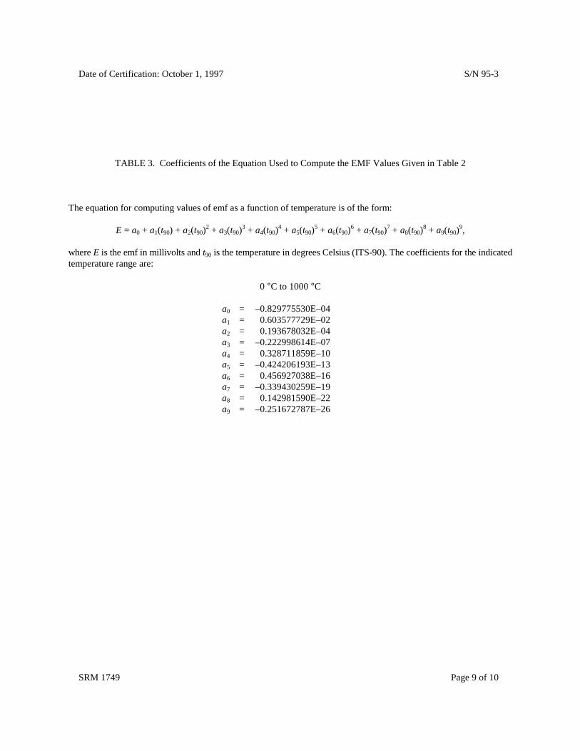
Date of Certification: October 1, 1997 S/N 95-3

SRM 1749 Page 9 of 10

TABLE 3. Coefficients of the Equation Used to Compute the EMF Values Given in Table 2

The equation for computing values of emf as a function of temperature is of the form:

E = a0 + a1(t90) + a2(t90)2 + a3(t90)3 + a4(t90)4 + a5(t90)5 + a6(t90)6 + a7(t90)7 + a8(t90)8 + a9(t90)9,

where E is the emf in millivolts and t90 is the temperature in degrees Celsius (ITS-90). The coefficients for the indicatedtemperature range are:

0 °C to 1000 °C

a0 = –0.829775530E–04a1 = 0.603577729E–02a2 = 0.193678032E–04a3 = –0.222998614E–07a4 = 0.328711859E–10a5 = –0.424206193E–13a6 = 0.456927038E–16a7 = –0.339430259E–19a8 = 0.142981590E–22a9 = –0.251672787E–26

Date of Certification: October 1, 1997 S/N 95-3

SRM 1749 Page 10 of 10

Figure 1: This figure shows the deviation of the emf of the Au/Pt thermocouple from an emf/temperature referencefunction for Au/Pt thermocouples given in Reference [3]. The deviation equals the thermocouple emf minusthe reference function emf. The dots denote measured values and the solid curve is calculated from apolynomial fitted to the data by the method of least squares. The dashed lines indicate an emf deviationequivalent to 0.05 °C

-2

-1

0

1

2

0 200 400 600 800 1000

Temperature / °C

EM

F D

evia

tion

/ µV

V

50 m°C

−50 m°C