Standard Operating Procedures for under ice ... - USGS · discharge measurements using ADCPs ....

1 qSOP-NA041-02-2015 Under ice discharge measurements using ADCPs

Standard Operating Procedures for under ice discharge measurements using ADCPs Water Survey of Canada P Campbell, Water Survey of Canada, Environment Canada, Ottawa, 2015

Version 2


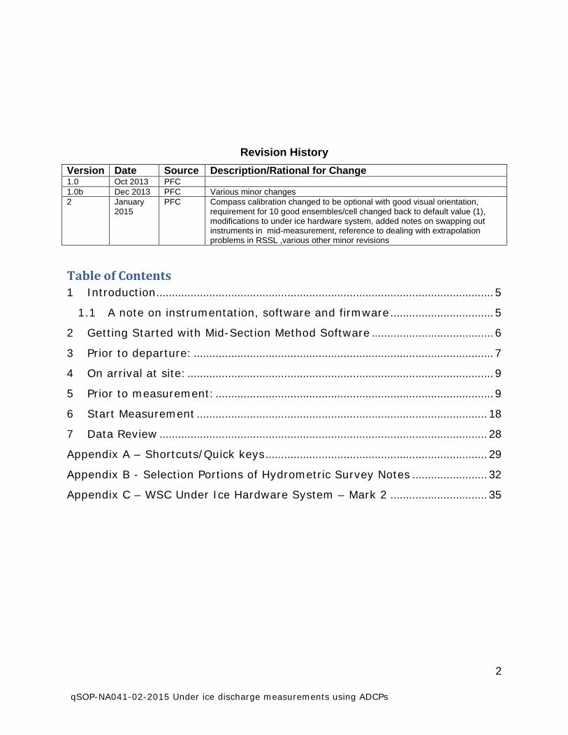
Revision History Version Date Source Description/Rational for Change 1.0 Oct 2013 PFC 1.0b Dec 2013 PFC Various minor changes 2 January

2015 PFC Compass calibration changed to be optional with good visual orientation,

requirement for 10 good ensembles/cell changed back to default value (1), modifications to under ice hardware system, added notes on swapping out instruments in mid-measurement, reference to dealing with extrapolation problems in RSSL ,various other minor revisions

Table of Contents 1 Introduction............................................................................................................ 5

1.1 A note on instrumentation, software and firmware ................................. 5

2 Getting Started with Mid-Section Method Software ....................................... 6

3 Prior to departure: ................................................................................................ 7

4 On arrival at site: .................................................................................................. 9

5 Prior to measurement: ......................................................................................... 9

6 Start Measurement ............................................................................................. 18

7 Data Review ......................................................................................................... 28

Appendix A – Shortcuts/Quick keys ....................................................................... 29

Appendix B - Selection Portions of Hydrometric Survey Notes ........................ 32

Appendix C – WSC Under Ice Hardware System – Mark 2 ............................... 35


Figure 1 – Example of a StreamPro mount. ........................................................... 8 Figure 2 – Mount for the S5/M9 and RiverRay w/ alignment tool ..................... 8 Figure 3 - Diagram of under ice deployment and ADCP depth ......................... 10 Figure 4 - RiverRay new measurement/measurement wizard form ................ 11 Figure 5 - Beam orientation for TRDI SxS Pro applications .............................. 12 Figure 6 - SxS Pro Measurement Wizard form for StreamPro .......................... 13 Figure 7 - ADCP setup for Rio Grande (left) and RiverRay (right) ................... 13 Figure 8 - Processing interface for SxS Pro .......................................................... 14 Figure 9 - RSSL Start Page ...................................................................................... 16 Figure 10 - Use slush remover to clear holes ...................................................... 18 Figure 11 - 1.5m Slush Remover with depth markings ..................................... 19 Figure 12 - Setup form for typical vertical ........................................................... 20 Figure 13 - Example of a StreamPro measurement in clear water .................. 21 Figure 14 - Station details within RSSL................................................................. 22 Figure 15 - Example of M9 display with slush. .................................................... 23 Figure 16 - An example of M9 output without slush. ......................................... 23 Figure 17 - Example low SNR profile in RSSL w/out beam obstructions ........ 24 Figure 18 - Example SNR profile in RSSL w beam obstruction ....................... 24 Figure 19 - Example SxS Pro of Intensity Profile w no beam obstructions .... 25 Figure 20 - End measurement form....................................................................... 27 Figure 21 – Two different under ice velocity profiles . ....................................... 29 Figure 22 – Example common extrapolation problem in RSSL. ....................... 29 Figure 23 - Keyed winter rod set ............................................................................ 36 Figure 24 - Base section with threaded meter mount. ...................................... 36 Figure 25 - First section single "dot" key. ............................................................ 36 Figure 26 - Second section double "dot" key....................................................... 37 Figure 27 - Third section triple "dot" key ............................................................. 37 Figure 28 - First section and orientation line connected.................................... 37 Figure 30 -Tool with upstream/downstream orientation line ............................ 38 Figure 31 - Price Current Meter threaded on winter rod ................................... 39 Figure 32 - FlowTracker ADV mount ...................................................................... 40 Figure 33 - FlowTracker mount on winter rod threaded base .......................... 40 Figure 34 - StreamPro adapter. .............................................................................. 41 Figure 35 - StreamPro mounted with orientation tool in place ........................ 41 Figure 36 - RiverRay mount showing 3/DS alignment stamp. ......................... 42


Figure 37 - RiverRay mount with orientation tool in place ................................ 42 Figure 38 - RiverRay mount with positioning hook (0.1 m1m offset) ............ 43 Figure 40 – M9 mount with positioning hook (0.1 m1m offset)....................... 44 Figure 41 - Standard transport case configuration for all adapters. ............... 45

Acknowledgements:

The creation of this document owes much to previous work done by people within the public and private sectors. Nick Stasulis of the USGS has had a significant role in promoting the standardization of procedures for using hydroacoustics under ice and in improving this document. Several people within the Water Survey of Canada have contributed to the development of these operating procedures including Scott Hill, Jeff Woodward, Murray Jones, Dustin DeWulf, Roger Pilling and Elizabeth Jamieson. Many more contributed to improving the operating procedures through hydroacoustics winter workshops. Canadian representatives for the major hydroacoustics manufacturers as well as technical representatives from the same manufacturers had played an active role in identifying improvements to hardware and software at Environment Canada- sponsored under ice hydroacoustics workshops.


1 Introduction Acoustic Doppler current profilers (ADCPs) are typically used for measuring river discharge from moving boats. However, specialized software now allow these instruments to be deployed to measure discharge using the mid-section method.

There are several reasons for using an ADCP in mid-section mode, including;

• Under- ice measurements • Poor bottom tracking performance combined with poor GPS reception or suspect compass

performance • Difficulty completing moving boat transects • Confirming edge discharges/bank overflow • Check measurements

This document presents guidance and standard operating procedures specific to deploying ADCPs for under ice measurements.

It is important to note that the mid-section method standards and procedures defined in the Hydrometric Field Manual- Measurement of Streamflow (Terzi, 1981) apply to under ice ADCP measurements unless otherwise stated in this document. Desirable characteristics of measurement cross sections for hydroacoustics under ice are similar to a good cross section for a mechanical ice meter measurement. The minimum required number of verticals for a measurement and limits for the maximum percentage of total discharge per vertical all remain unchanged for ADCP under ice measurements.

Safety protocol for under ice measurements are beyond the scope of this document. Readers are referred to the Water Survey of Canada Occupational Safety and Health Policy for Working on Ice and the Ice Surface Safety Training Manual for more complete references on ice safety. Current versions of these documents are available on the Water Survey of Canada (WSC) Intranet Library.

1.1 A note on instrumentation, software and firmware A variety of ADCP types may be used for under ice measurements, and depending on the manufacturer, the mid-section discharge measurement software will also vary. Currently (2015) the software approved for under ice ADCP measurements for WSC operations are SonTek YSI’s RiverSurveyor Stationary Live (RSSL) and Teledyne RDI’s Section by Section Pro (SxS Pro).

Be aware that the specified minimum storage temperatures are -20°C for TRDI ADCPs and -10°C for the M9/S5 so it is important to avoid exposing an uncovered ADCP to very cold air (-20°C or colder) for extended periods. Suggestions for protecting ADCPs in cold weather are included in section 4 of this document. There have been documented cases of cold-weather induced damage occurring to the


StreamPro ADCP so particular care should be taken to ensure storage temperatures for the StreamPro are not below specified temperatures.

The procedures and guidelines presented in this document are described in the context of each of the two primary software packages. Both have detailed, searchable user guides and help functions accessible within the software. Consult them regularly to learn more beyond this document. For a list of the current versions of approved software and firmware, please consult qREC-NA058-201x Recommended Hydroacoustic Software and Firmware for WSC document which can be found on the WSC Ecollab Library.

2 Getting Started with Mid-Section Method Software SonTek YSI’s RiverSurveyor Stationary Live (RSSL) and Teledyne RDI’s Section by Section Pro (SxS Pro) are two examples of software that allow mid-section methods to be applied with ADCPs.

Information specific to SonTek YSI (SonTek) and Teledyne RDI (TRDI) are identified in separate boxes. SonTek information is highlighted in grey. Information specific to TRDI is not highlighted.

Both RSSL and SxS Pro software are free, allowing review of existing measurements by anyone with a PC. However some form of registration key is required for RSSL and SxS Pro to acquire data in mid-section mode.

TRDI: All Water Survey of Canada ADCP’s acquired through the National Individual Standing Offer are delivered configured for mid-section capabilities and each has an assigned unique Section by Section Pro key to unlock the software for acquiring data. This key needs to be input into each PC operating Section-by-Section Pro Software for that ADCP. Open SxS Pro and select menu items Help/Register ADCP. It is recommended to display the Section-by-Section Pro key clearly on the exterior of any ADCP if a key exists for that instrument

Note: From 2007 to 2010 Teledyne RDI had supported section by section software bundled with WinRiver II software. WinRIver II section by section software distinct from Section by Section Pro, is unstable and no longer supported by TRDI. Therefore it is not approved and not recommended for use.

SonTek: To acquire data with River Surveyor Stationary Live software, a key is input into the ADCP firmware using utility software. Afterwards, any PC with RSSL software will function with the M9/S5 ADCP.

There are mobile and PDA versions of the mid-section method software for both SonTek and TRDI ADCPs. WSC does not recommend use of PDA/mobile/smart phone versions of the mid-section method software. Reasons for not recommending PDA based software for mid-section measurements include; difficulty in monitoring and reviewing measurements on smaller displays, limited technical support from manufacturers (no support from TRDI, little documentation from SonTek). Fewer software options will simplify the software testing process and reduce the number of problems around data quality and hardware compatibility.

http://nadm.ontario.int.ec.gc.ca/natmon/wsc/apps/wsclibrary/view_document-eng.cfm?ID=7591


3 Prior to departure: The following steps should be followed prior to data collection in the field:

1. Inspect ADCP transducer face(s), cables and connectors for damage. 2. Confirm:

• communication with ADCP works by establishing communication through the mid-section software

• the ADCP is suitable for the expected effective depths, For example the RiverRay typically requires 0.75m effective depth or more. The

M9 typically requires at least 0.4m effective depth (note that the M9 should have a screening distance that extends 16 cm beyond the transducers). Be aware that there can be attenuation of the range for both the RiverRay and M9/S5 in low backscatter conditions associated with cold clear water.

StreamPro or S5 are best for consistently shallow effective depths, but like all ADCP’s they can experience attenuation of signals in cold, clear water. Although a StreamPro may profile to 6 m depths in ideal conditions, in winter measurements the range may be limited to less than 3.0 m.

• firmware and software versions are up-to-date. Current listings for WSC can be found in WSC library (qREC-NA058-201x: Recommended Hydroacoustic Software and Firmware for WSC).

• Auger flighting will drill holes large enough for the ADCP to be used • Batteries or battery packs are fully charged

3. Run system tests 4. Check the ADCP mount:

• The mount should not allow the ADCP to spin or otherwise allow the ADCP orientation to change without the knowledge of the operator.

• The mount should have a visual alignment tool (Fig. 2) to check orientation of ADCP with respect to the measurement section. Ensure there is a way to check that the rod is held in the vertical position with pitch and roll near zero degrees (e.g. a fish eye bubble attached to the rod).

• The mount must be constructed of non-ferrous material. • Depth markings, which should be offset relative to the transducer, must be accurate and easily

readable. • Have the communicaton/power cables suitable for under ice measurements ready. For the

RiverRay and M9/S5, these are cables with 90 degree connectors, (a 3 m extension cable in the case of the RiverRay), that allow passage of the unit through the holes. If using a StreamPro be sure to have a 2.5 m extension cable .

http://nadm.ontario.int.ec.gc.ca/natmon/wsc/apps/wsclibrary/view_document-eng.cfm?ID=7591


Figure 1 – Example of a StreamPro mount. When the horizontal plate is held up against the underside of the ice, the transducers are at a known depth below the ice.

Figure 2 – Mount for the S5/M9 and RiverRay w/ alignment tool

A 90 degree connector cable, available RiverRay and M9/S5, reduces the overall diameter of the instrument for passage through the hole. A standard, straight connector can be used but requires drilling larger holes, possibly exposing the connector to damage with repeated use through the ice. To use a StreamPro under ice, you will require the 2.5 m extension cable.

SonTek: Since the orientation of the pins on the face of the unit connector varies between individual ADCPs, it is necessary to have a custom 90 degree communication cable fabricated for specific units. You will need to submit a picture showing the connector pin orientation for the ADCP when ordering.


SonTek: The rechargeable battery pack within the PCM for the M9 is likely not sufficient for winter operation. It is recommended to pack an external power supply and a cable with an external power supply connector to supplement or replace the PCM battery pack.

4 On arrival at site: • The selected measurement cross section should have characteristics similar to a good

conventional measurement section. • Check battery voltages and replace if necessary • Immerse the ADCP in water to acclimatize the transducers and temperature sensor. It

may take a half hour or longer for the ADCP to adjust to near freezing temperatures. The specified minimum storage temperatures are -20°C for the RiverRay and -10°C for the M9/S5 so it is important to avoid exposing an uncovered ADCP to very cold air (-20°C or colder) for extended periods of time (>30 minutes). Consider using an insulated container with a hand warmer to protect the ADCP during transport. In the case of the StreamPro, where the electronics are external to the transducer head, it is recommended to keep the electronics housing in an insulated pack during the measurement when air temperatures are below -5C.

5 Prior to measurement: • Connect the ADCP to the PC com port, preferably to a USB to Serial port that is FTDI chipset

controlled and not a built-in DB9 serial port (COM1) on the notebook. Test the communications. • Set the ADCP time to the PC time. • Folder and file naming conventions.

o SxS Pro file name convention: StationID_YYYYMMDD.sxs.mmt. (folder can be named Station ID_YYYYMMDD.AQ#)

o RiverSurveyor Stationary Live folder name convention (Station ID_YYYYMMDD.SQ#). File is saved as YYYYMMDDmmss.sta within StationaryDataFiles subfolder. Other subfolders are CompassCal and SystemTest.

• If a suitable mounting system is used and the operator can visually confirm proper instrument alignment within approximately +/- 5 degrees with respect to the measuring section, calibration of the ADCP compass is not necessary.

o If, however, there is a concern about either the ability to visually confirm the instrument alignment or if there are potential problems maintaining a consistent instrument orientation throughout the measurement (i.e. concerns about the instrument rotating in the mount), then it is recommended to calibrate the compass. This gives the option to use either earth or instrument orientation references at a later time. Follow compass calibration procedures as recommended for moving boat measurements. As of late 2014, ISM compass calibration cannot be done within SxS Pro and must be done within WinRiver II. Note compass calibration results in field notes and comments section in electronic file and save calibration file with measurement file.

• Avoid risks of losing an instrument through a hole by securing it to an object such as a sled. Do not rely on the communication/power cable as a tether.

• Run diagnostic tests for ADCP


• Adjust ADCP data acquisition parameters : o Duration: 40 seconds is the standard data collection duration for mechanical current

meters and the default sampling period for SxS Pro. The software will prompt users to extend the sampling period if more than 25% of ensembles are missing. Use a minimum sampling time of 40 seconds. If less than 30 valid ensembles at a vertical are obtained within that period, increase the sampling time to obtain 30 valid ensembles.

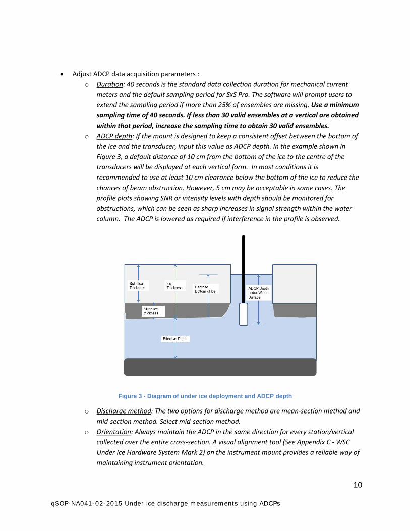
o ADCP depth: If the mount is designed to keep a consistent offset between the bottom of the ice and the transducer, input this value as ADCP depth. In the example shown in Figure 3, a default distance of 10 cm from the bottom of the ice to the centre of the transducers will be displayed at each vertical form. In most conditions it is recommended to use at least 10 cm clearance below the bottom of the ice to reduce the chances of beam obstruction. However, 5 cm may be acceptable in some cases. The profile plots showing SNR or intensity levels with depth should be monitored for obstructions, which can be seen as sharp increases in signal strength within the water column. The ADCP is lowered as required if interference in the profile is observed.

Figure 3 - Diagram of under ice deployment and ADCP depth

o Discharge method: The two options for discharge method are mean-section method and mid-section method. Select mid-section method.

o Orientation: Always maintain the ADCP in the same direction for every station/vertical collected over the entire cross-section. A visual alignment tool (See Appendix C - WSC Under Ice Hardware System Mark 2) on the instrument mount provides a reliable way of maintaining instrument orientation.


o Vertical Sample: A minimum of 2 depth cells must be obtained at every vertical. For non-auto adapting TRDI ADCPs, it may be necessary to change the configuration at shallow verticals. A note on changing configurations during a measurement is in the dialog box below.

TRDI: Measurement configuration

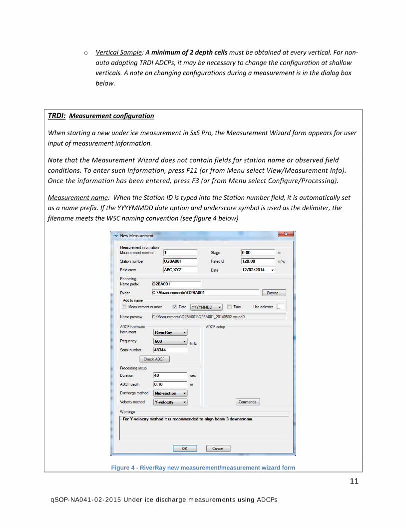
When starting a new under ice measurement in SxS Pro, the Measurement Wizard form appears for user input of measurement information.

Note that the Measurement Wizard does not contain fields for station name or observed field conditions. To enter such information, press F11 (or from Menu select View/Measurement Info). Once the information has been entered, press F3 (or from Menu select Configure/Processing).

Measurement name: When the Station ID is typed into the Station number field, it is automatically set as a name prefix. If the YYYYMMDD date option and underscore symbol is used as the delimiter, the filename meets the WSC naming convention (see figure 4 below)

Figure 4 - RiverRay new measurement/measurement wizard form


Data Acquisition Parameters setup in Measurement Wizard

Duration: If less than 75% of ensembles (i.e. < 30/40) are valid at the end of a sampling period, the operator will be asked if they wish to extend the duration of the data collection period. It is recommended to obtain a minimum of 30 valid and consistent ensembles at each station/vertical. A 40 second sampling period will be sufficient for most deployments.

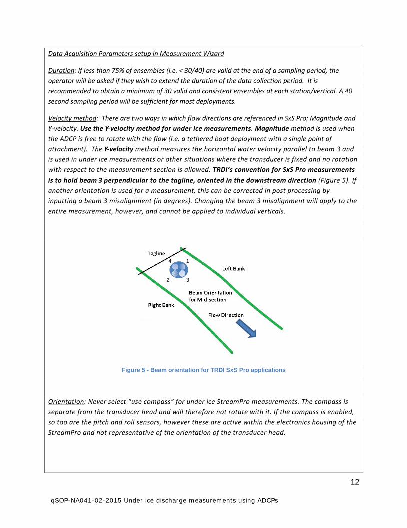
Velocity method: There are two ways in which flow directions are referenced in SxS Pro; Magnitude and Y-velocity. Use the Y-velocity method for under ice measurements. Magnitude method is used when the ADCP is free to rotate with the flow (i.e. a tethered boat deployment with a single point of attachment). The Y-velocity method measures the horizontal water velocity parallel to beam 3 and is used in under ice measurements or other situations where the transducer is fixed and no rotation with respect to the measurement section is allowed. TRDI’s convention for SxS Pro measurements is to hold beam 3 perpendicular to the tagline, oriented in the downstream direction (Figure 5). If another orientation is used for a measurement, this can be corrected in post processing by inputting a beam 3 misalignment (in degrees). Changing the beam 3 misalignment will apply to the entire measurement, however, and cannot be applied to individual verticals.

Figure 5 - Beam orientation for TRDI SxS Pro applications

Orientation: Never select “use compass” for under ice StreamPro measurements. The compass is separate from the transducer head and will therefore not rotate with it. If the compass is enabled, so too are the pitch and roll sensors, however these are active within the electronics housing of the StreamPro and not representative of the orientation of the transducer head.

4

3

1

2


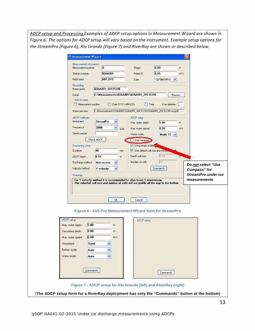
ADCP setup and Processing Examples of ADCP setup options in Measurement Wizard are shown in Figure 6. The options for ADCP setup will vary based on the instrument. Example setup options for the StreamPro (Figure 6), Rio Grande (Figure 7) and RiverRay are shown or described below.

Figure 6 - SxS Pro Measurement Wizard form for StreamPro

Figure 7 - ADCP setup for Rio Grande (left) and RiverRay (right)

(The ADCP setup form for a RiverRay deployment has only the “Commands” button at the bottom)

Do not select “Use Compass” for StreamPro under ice measurements


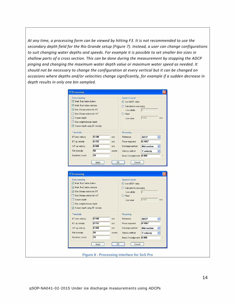
At any time, a processing form can be viewed by hitting F3. It is not recommended to use the secondary depth field for the Rio Grande setup (Figure 7). Instead, a user can change configurations to suit changing water depths and speeds. For example it is possible to set smaller bin sizes in shallow parts of a cross section. This can be done during the measurement by stopping the ADCP pinging and changing the maximum water depth value or maximum water speed as needed. It should not be necessary to change the configuration at every vertical but it can be changed on occasions where depths and/or velocities change significantly, for example if a sudden decrease in depth results in only one bin sampled.

Figure 8 - Processing interface for SxS Pro


The default setting for minimum number of good ensembles for a cell is 1. This means that if only one velocity sample over 40 seconds is available for a given cell depth, this cell will still be used in the determination of the average water velocity for the vertical.

The default setting for 3 beam solution for water tracking (WT) is “not activated”. It may be useful to activate 3 beam solution for water tracking if there is suspected interference with one of the 4 beams (for example irregular slush/ice depths or vertical walls).

Beam 3 misalignment: The convention for the Y-velocity method in SxS Pro is to hold the ADCP with beam 3 facing downstream (Figure 5). If, for example, a user inadvertently set beam 3 facing upstream, they could correct for the misalignment by setting the beam 3 misalignment to 180 degrees. Since the beam 3 misalignment factor is applied to all verticals, you can change the beam 3 misalignment value during the measurement but maintain a consistent orientation during the measurement so the orientation is corrected by the software. Note in the software comments section and survey notes why the misalignment factor is applied. Since the transducer for the RiverRay is oriented at a 45 degree offset from the direction of the impulse connector, there is a greater likelihood of holding beam three misaligned either at 45 degrees or 320 degrees from the intended orientation, especially if using a mount without beam 3 orientation displayed clearly. In these cases, changing the beam 3 misalignment factor in post-processing should resolve the problem.


SonTek: When creating a new measurement in RiverSurveyor Stationary Live, you are presented with the main page from which you select connect to RiverSurveyor system. Once connected, the Start Page appears (Figure 9). Enter the site information.

Figure 9 - RSSL Start Page


Orientation: If the M9/S5 is properly mounted and deployed using a reasonably accurate visual alignment tool, it is not required to obtain the tagline azimuth and complete a compass calibration. In this case, use the XYZ, or instrument orientation reference for all stations.

Set the ADCP time. Run the system test. Under “Change System Settings”, recommended settings are “System” for track reference and “Vertical Beam” for depth reference, Mid-Section for discharge method and Smart Pulse is enabled.

Once the transducer is set through the first hole, run the beam check feature to confirm if SNR values are consistent between the different beams and there are no obvious obstacles near the face of the transducers. Users should select the 3MHz frequency in shallow conditions for the beam check.


6 Start Measurement For under ice conditions, confirm ADCP reported water temperature reads between -2 and 2 degrees Celsius. If the ADCP displayed temperature does not fall within this range, wait until the ADCP temperature stabilizes to within this range. If there is a suspected broken thermistor, confirm water temperatures independently with a thermometer and override the ADCP temperatures with a manually input value.

Once Start Measurement is selected, you are prompted for starting edge information. Both SxS Pro and RSSL prompts for starting bank (left or right), distance from IP, edge depth and velocity correction factor. The velocity correction factor allows the user to input an estimated water velocity at an edge section as a percentage of the closest measured velocity. The default velocity correction factor is one for RSSL and zero for SxS Pro. Either value is suitable when there is a sloping bank resulting in a depth of zero at the edge. Often a measurement may start (or terminate with a vertical wall. As with moving boat measurements the nearest measured vertical (or station) would be at a distance approximately equal to the depth at the wall and in this case a typical correction factor for the velocity at the wall or pier with a smooth surface is 0.65. This correction factor would be reduced with increasing wall/pier roughness.

When edge information is complete, go to the first vertical beyond the edge of water.

TRDI: SxS Pro labels the starting edge as Vertical 1. After the starting edge information is input the unit starts pinging. Place the ADCP in the first hole (vertical 2) for a water velocity measurement and verify if the measured velocity is valid by monitoring the lower left portion of the tabular output. At this point you will have to input the velocity profile type, in this case “Ice (no-slip/no-slip)”.

SonTek: RSSL labels the starting edge as Station 1. Users will be prompted to input the water surface type (i.e. open water or under ice measurement) only after inputting the starting bank information.

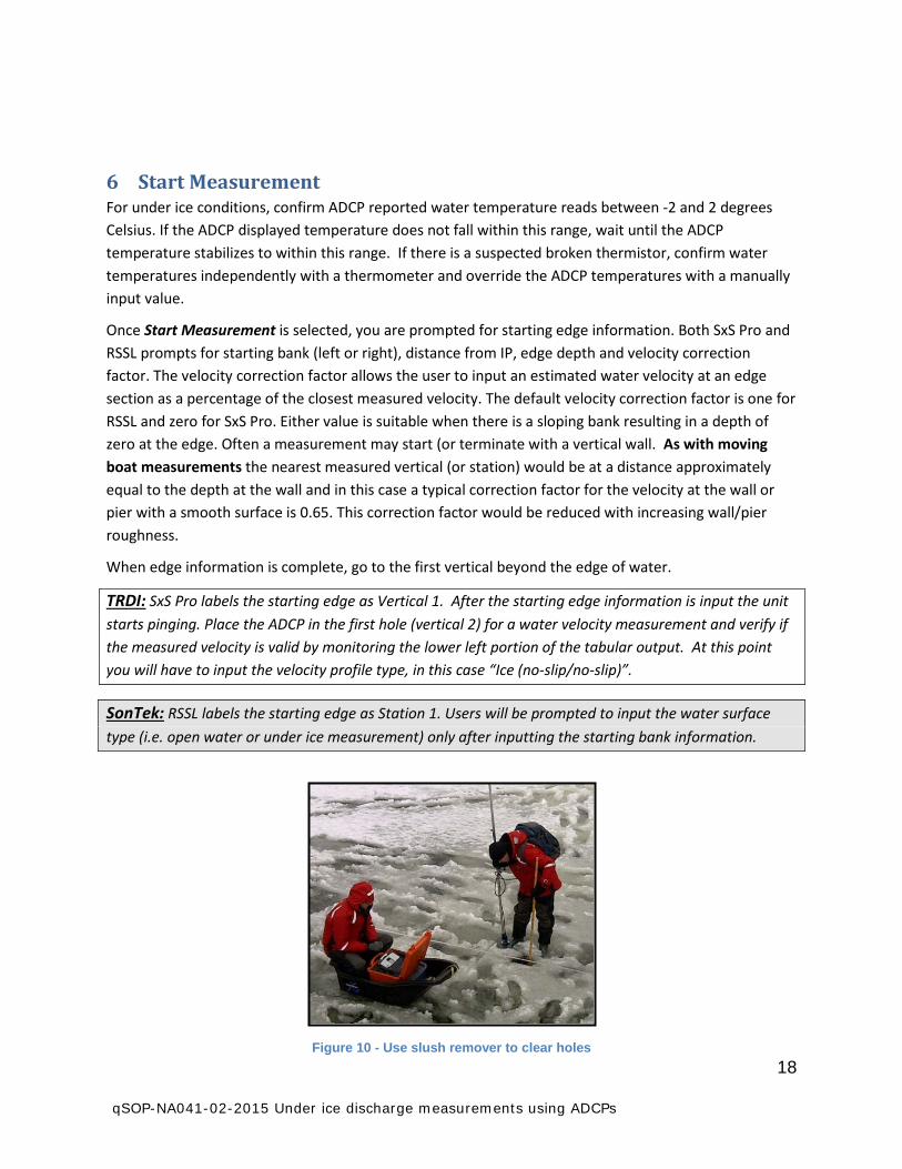
Figure 10 - Use slush remover to clear holes


At the first hole you are prompted for velocity profile type in SxS Pro (choose “Ice”) or water surface type in RSSL (choose ice or ice + slush), tagline position, ice thickness, depth to bottom of ice, depth to bottom of slush (if applicable) and distance of ADCP below ice/slush horizon. Although a final discharge requires only the distance below the ice, it is recommended to complete all applicable fields. This will ensure displayed graphics in the software interface are consistent with actual conditions.

Positioning hooks for the measurement of ice thickness (0.1 metre offset) have been developed as part River Ray and M9/S5 ADCP adapters. Use of these measurement hooks should be done with caution to avoid wear on connectors or communication cables. It is recommended that the WSC Slush Remover or a similar measurement tool be used to determine ice thickness instead the ADCP itself.

Figure 11 - 1.5m WSC Slush Remover with depth markings

If slush is present, it will be necessary to lower the ADCP into the water while pinging until valid data is generated. Try not the set the position of the instrument at exactly the level of the slush. Instead, set it below the slush to reduce potential interference with the acoustic signals. Water velocities should be sufficient to clear the slush from the ADCP transducer head. Depending on the mount, the user might feel the resistance of the slush on the horizontal part of the transducer bracket, indicating the depth of the slush below the water surface. Try not to pull the instrument back up into the slush once a clear signal is seen. Be aware that the transducer face is potentially the first surface in contact with a hard, unseen object. When probing through slush or in shallow conditions, be careful to not impact the transducer face on rock or ice surfaces.

If velocities can be measured but an accurate depth cannot be obtained due to weeds or high suspended sediment concentrations, both RSSL and SxS Pro have an option to manually input depths at a vertical/station. This depth value might be obtained by manual sounding or observing intermittent valid depths while pinging. Be careful when using manual depths in SxS Pro as the depth values from a manually input vertical can be carried forward to the next vertical as defaults.

Prior to starting data collection, set the ADCP to the upstream or downstream side of the hole, depending on the type of mount, and confirm alignment with the visual alignment tool. Check the mount is plumb. If an internal calibrated compass is also being used, check the ADCP heading at each station/vertical to ensure consistency. Select velocity profile for Ice and input the applicable thickness and depth measurements. Figure 12 provides an example for a typical vertical setup.


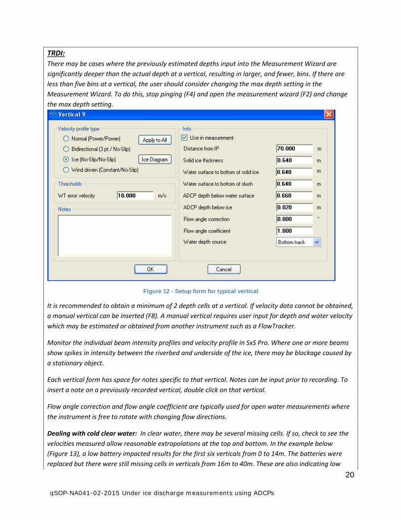
TRDI: There may be cases where the previously estimated depths input into the Measurement Wizard are significantly deeper than the actual depth at a vertical, resulting in larger, and fewer, bins. If there are less than five bins at a vertical, the user should consider changing the max depth setting in the Measurement Wizard. To do this, stop pinging (F4) and open the measurement wizard (F2) and change the max depth setting.

Figure 12 - Setup form for typical vertical

It is recommended to obtain a minimum of 2 depth cells at a vertical. If velocity data cannot be obtained, a manual vertical can be inserted (F8). A manual vertical requires user input for depth and water velocity which may be estimated or obtained from another instrument such as a FlowTracker.

Monitor the individual beam intensity profiles and velocity profile in SxS Pro. Where one or more beams show spikes in intensity between the riverbed and underside of the ice, there may be blockage caused by a stationary object.

Each vertical form has space for notes specific to that vertical. Notes can be input prior to recording. To insert a note on a previously recorded vertical, double click on that vertical.

Flow angle correction and flow angle coefficient are typically used for open water measurements where the instrument is free to rotate with changing flow directions.

Dealing with cold clear water: In clear water, there may be several missing cells. If so, check to see the velocities measured allow reasonable extrapolations at the top and bottom. In the example below (Figure 13), a low battery impacted results for the first six verticals from 0 to 14m. The batteries were replaced but there were still missing cells in verticals from 16m to 40m. These are also indicating low


correlation counts (<50 counts) in the profile view (to switch between correlation or intensity information, right click on profile view). Correlation is low when the ADCP cannot match echo patterns reflected from the backscattering particles in subsequent phase measurements. The low correlation in this case is related to the lack of backscatters in the water column and the low correlation should be mirrored by low intensities as well in this case. More energy can be input into the water by increasing the cell size or increasing the voltage to the StreamPro (it will handle up to 18v). In the measurement below (Figure 13), the sampling time was increased from 40 seconds to 80 seconds at the 40m mark and as a result, fewer cells were missing. Finally, users might consider lowering the transducer to sample the middle portion of the velocity profile instead of just the upper portion.

Figure 13 - Example of a StreamPro measurement in clear water, where default configuration settings were

changed to optimize data quality.

If low backscatter conditions (<70dB) are encountered while using the RiverRay, monitor for unexpectedly low discharge values. Although RiverRay firmware v44.13 and up is expected to have resolved a low backscatter bias, there have been occasional reports within the USGS of low bias in low backscatter conditions, possibly caused by interference from external sources. In cases where there are limited velocity samples (3 or less) in cells, there may be an impact on the quality of the extrapolation for that vertical. Check the velocity contour plot to see if any outlier velocities are present in cells near the top or bottom of the measured portion. If there are outlier velocities, the number of good ensembles in a cell can be increased from 1 to 3 or 4 or the vertical can be repeated. This will prevent unreasonable extrapolations from small numbers of velocity samples.


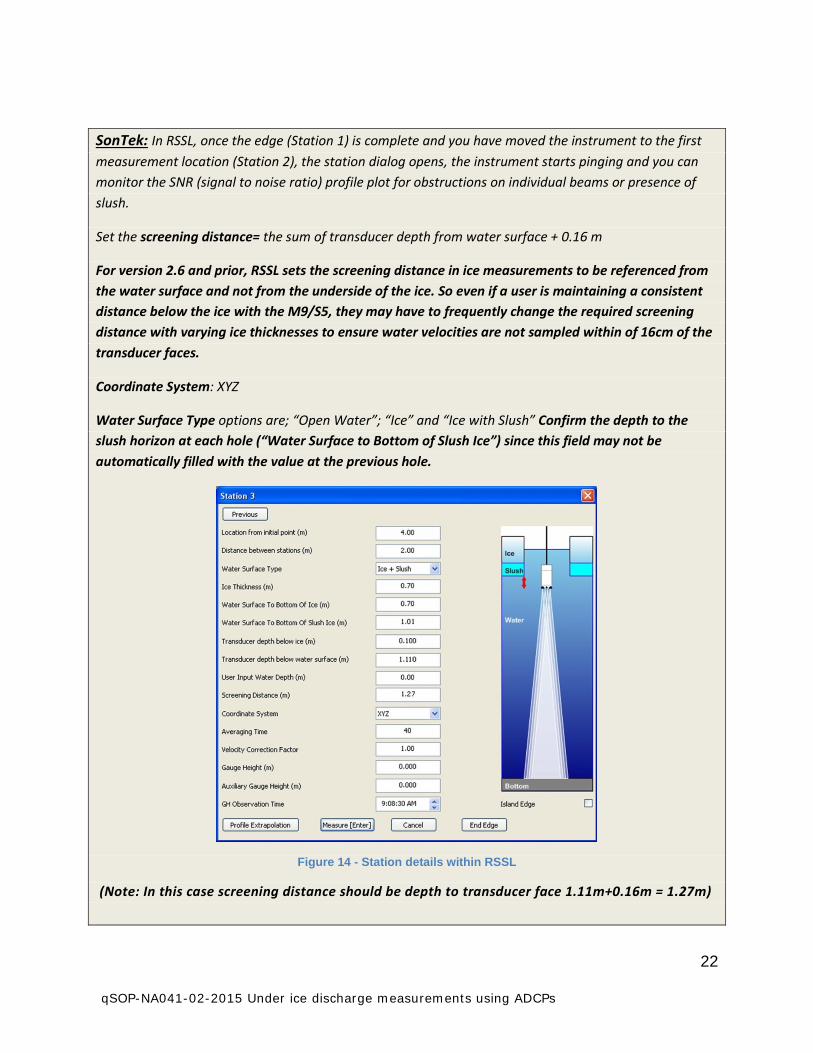
SonTek: In RSSL, once the edge (Station 1) is complete and you have moved the instrument to the first measurement location (Station 2), the station dialog opens, the instrument starts pinging and you can monitor the SNR (signal to noise ratio) profile plot for obstructions on individual beams or presence of slush.

Set the screening distance= the sum of transducer depth from water surface + 0.16 m

For version 2.6 and prior, RSSL sets the screening distance in ice measurements to be referenced from the water surface and not from the underside of the ice. So even if a user is maintaining a consistent distance below the ice with the M9/S5, they may have to frequently change the required screening distance with varying ice thicknesses to ensure water velocities are not sampled within of 16cm of the transducer faces.

Coordinate System: XYZ

Water Surface Type options are; “Open Water”; “Ice” and “Ice with Slush” Confirm the depth to the slush horizon at each hole (“Water Surface to Bottom of Slush Ice”) since this field may not be automatically filled with the value at the previous hole.

Figure 14 - Station details within RSSL

(Note: In this case screening distance should be depth to transducer face 1.11m+0.16m = 1.27m)


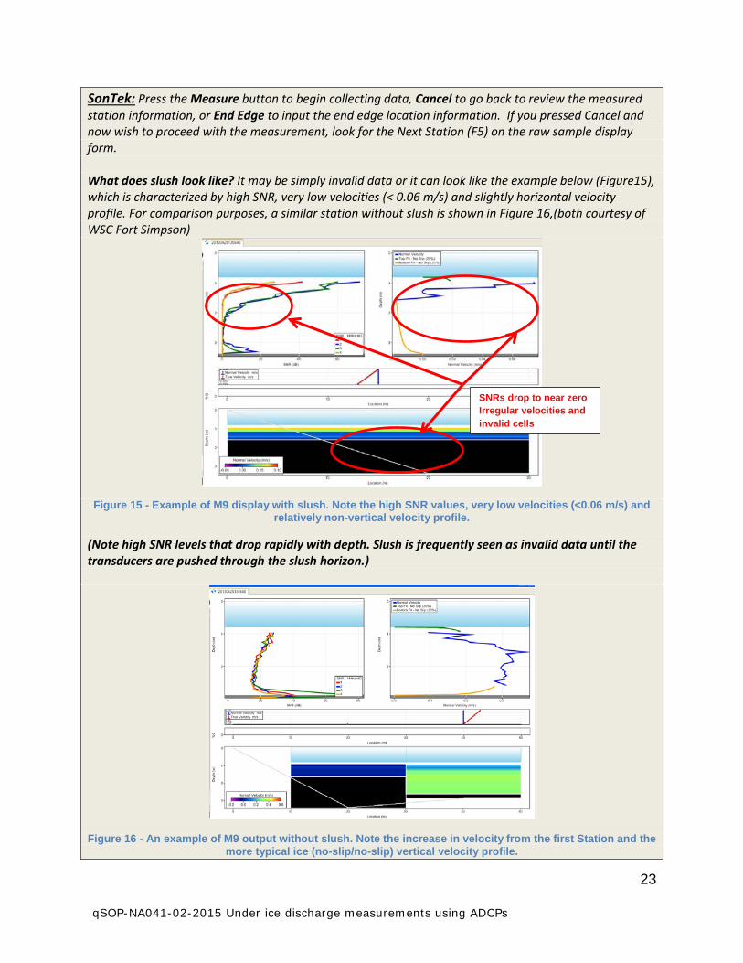
SonTek: Press the Measure button to begin collecting data, Cancel to go back to review the measured station information, or End Edge to input the end edge location information. If you pressed Cancel and now wish to proceed with the measurement, look for the Next Station (F5) on the raw sample display form. What does slush look like? It may be simply invalid data or it can look like the example below (Figure15), which is characterized by high SNR, very low velocities (< 0.06 m/s) and slightly horizontal velocity profile. For comparison purposes, a similar station without slush is shown in Figure 16,(both courtesy of WSC Fort Simpson)

Figure 15 - Example of M9 display with slush. Note the high SNR values, very low velocities (<0.06 m/s) and relatively non-vertical velocity profile.

(Note high SNR levels that drop rapidly with depth. Slush is frequently seen as invalid data until the transducers are pushed through the slush horizon.)

Figure 16 - An example of M9 output without slush. Note the increase in velocity from the first Station and the more typical ice (no-slip/no-slip) vertical velocity profile.

SNRs drop to near zero Irregular velocities and invalid cells


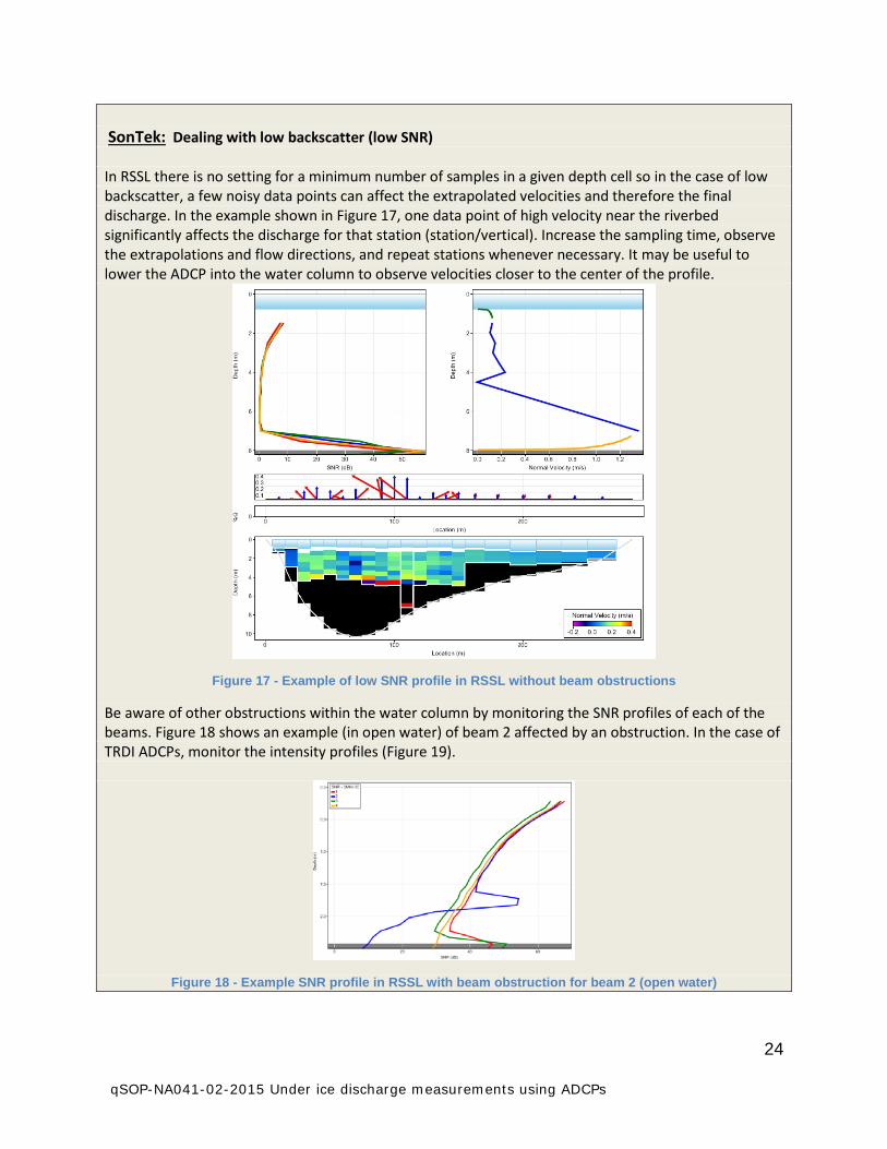
SonTek: Dealing with low backscatter (low SNR) In RSSL there is no setting for a minimum number of samples in a given depth cell so in the case of low backscatter, a few noisy data points can affect the extrapolated velocities and therefore the final discharge. In the example shown in Figure 17, one data point of high velocity near the riverbed significantly affects the discharge for that station (station/vertical). Increase the sampling time, observe the extrapolations and flow directions, and repeat stations whenever necessary. It may be useful to lower the ADCP into the water column to observe velocities closer to the center of the profile.

Figure 17 - Example of low SNR profile in RSSL without beam obstructions

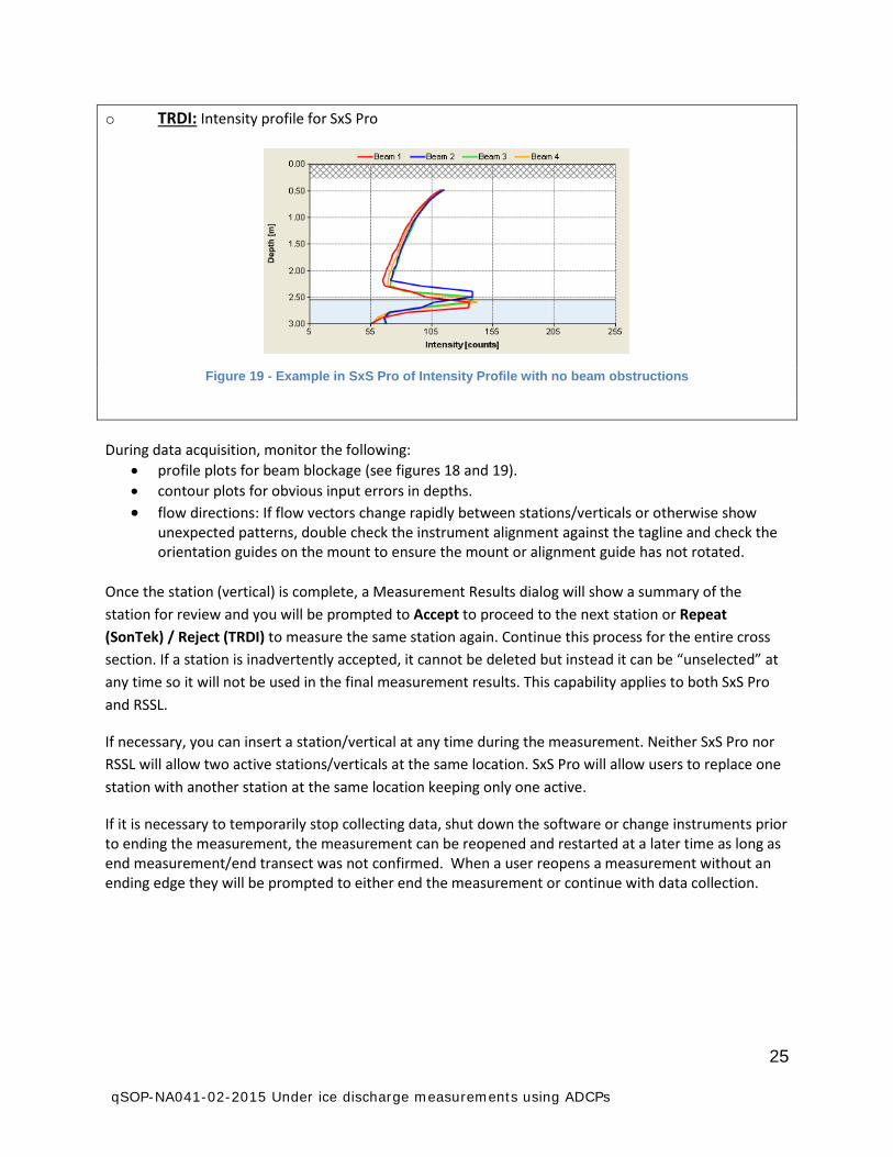
Be aware of other obstructions within the water column by monitoring the SNR profiles of each of the beams. Figure 18 shows an example (in open water) of beam 2 affected by an obstruction. In the case of TRDI ADCPs, monitor the intensity profiles (Figure 19).

Figure 18 - Example SNR profile in RSSL with beam obstruction for beam 2 (open water)


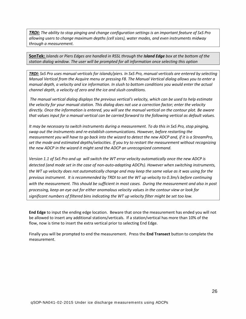
o TRDI: Intensity profile for SxS Pro

Figure 19 - Example in SxS Pro of Intensity Profile with no beam obstructions

During data acquisition, monitor the following:

• profile plots for beam blockage (see figures 18 and 19). • contour plots for obvious input errors in depths. • flow directions: If flow vectors change rapidly between stations/verticals or otherwise show

unexpected patterns, double check the instrument alignment against the tagline and check the orientation guides on the mount to ensure the mount or alignment guide has not rotated.

Once the station (vertical) is complete, a Measurement Results dialog will show a summary of the station for review and you will be prompted to Accept to proceed to the next station or Repeat (SonTek) / Reject (TRDI) to measure the same station again. Continue this process for the entire cross section. If a station is inadvertently accepted, it cannot be deleted but instead it can be “unselected” at any time so it will not be used in the final measurement results. This capability applies to both SxS Pro and RSSL.

If necessary, you can insert a station/vertical at any time during the measurement. Neither SxS Pro nor RSSL will allow two active stations/verticals at the same location. SxS Pro will allow users to replace one station with another station at the same location keeping only one active.

If it is necessary to temporarily stop collecting data, shut down the software or change instruments prior to ending the measurement, the measurement can be reopened and restarted at a later time as long as end measurement/end transect was not confirmed. When a user reopens a measurement without an ending edge they will be prompted to either end the measurement or continue with data collection.


TRDI: The ability to stop pinging and change configuration settings is an important feature of SxS Pro allowing users to change maximum depths (cell sizes), water modes, and even instruments midway through a measurement. SonTek: Islands or Piers Edges are handled in RSSL through the Island Edge box at the bottom of the station dialog window. The user will be prompted for all information once selecting this option TRDI: SxS Pro uses manual verticals for islands/piers. In SxS Pro, manual verticals are entered by selecting Manual Vertical from the Acquire menu or pressing F8. The Manual Vertical dialog allows you to enter a manual depth, a velocity and ice information. In slush to bottom conditions you would enter the actual channel depth, a velocity of zero and the ice and slush conditions.

The manual vertical dialog displays the previous vertical's velocity, which can be used to help estimate the velocity for your manual station. This dialog does not use a correction factor; enter the velocity directly. Once the information is entered, you will see the manual vertical on the contour plot. Be aware that values input for a manual vertical can be carried forward to the following vertical as default values. It may be necessary to switch instruments during a measurement. To do this in SxS Pro, stop pinging, swap out the instruments and re-establish communications. However, before restarting the measurement you will have to go back into the wizard to detect the new ADCP and, if it is a StreamPro, set the mode and estimated depths/velocities. If you try to restart the measurement without recognizing the new ADCP in the wizard it might send the ADCP an unrecognized command. Version 1.1 of SxS Pro and up will switch the WT error velocity automatically once the new ADCP is detected (and mode set in the case of non-auto-adapting ADCPs). However when switching instruments, the WT up velocity does not automatically change and may keep the same value as it was using for the previous instrument. It is recommended by TRDI to set the WT up velocity to 0.3m/s before continuing with the measurement. This should be sufficient in most cases. During the measurement and also in post processing, keep an eye out for either anomalous velocity values in the contour view or look for significant numbers of filtered bins indicating the WT up velocity filter might be set too low.

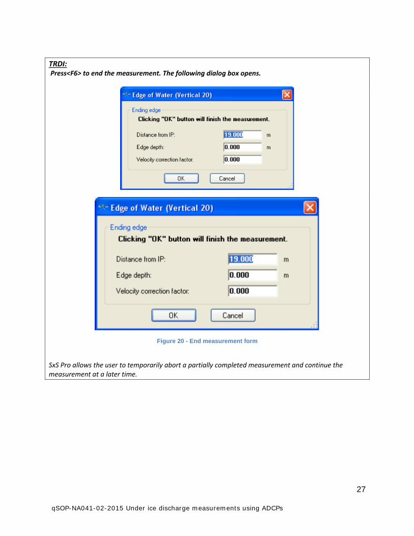
End Edge to input the ending edge location. Beware that once the measurement has ended you will not be allowed to insert any additional stations/verticals. If a station/vertical has more than 10% of the flow, now is time to insert the extra vertical prior to selecting End Edge. Finally you will be prompted to end the measurement. Press the End Transect button to complete the measurement.


TRDI: Press<F6> to end the measurement. The following dialog box opens.

Figure 20 - End measurement form

SxS Pro allows the user to temporarily abort a partially completed measurement and continue the measurement at a later time.


7 Data Review Data must be first thoroughly reviewed while still in the field to identify and correct any potential acquisition error. Use the Hydrometric survey notes to conduct a thorough field review prior to leaving the site. Among the listed items within the survey note, check:

• Diagnostic test results OK and logged. ADCP clock set. Temperature sensor valid. • Review contour plot as a visual check on input errors for ice thickness, depths, ADCP depth etc. • Look at flow vectors/flow direction to detect obvious inconsistencies or errors that may be

caused by procedural errors or problems with the ADCP mount. • Check minimum number of valid ensembles and sampling duration were achieved. • (SxS Pro only) Are there several missing cells within the station/vertical? If so, check to see if the

velocities measured allow reasonable extrapolations at the top and bottom. In clear water, there may be several missing cells. This is shown as correlation profiles dropping to noise floor level and staying at those levels (60 counts or lower for RiverRay, 85 or lower for StreamPro) It may be necessary to repeat the measurement with longer sampling times at each vertical and/or increasing the size of the bins or changing the water mode.

• SNR/intensity. Look for spikes caused by obstructions. • Click on individual stations/verticals to view extrapolated portions of profiles. Is there a

discontinuity of the measured profile? If so, you may need to adjust the exponents (to do this, see explanation below). In most cases, extrapolation settings are consistent among stations/verticals.

• Suitable number of verticals/stations and percentage of discharge per vertical/station The typical extrapolation method for under ice is no slip top /no slip bottom. The no slip method of extrapolation uses a power fit to force the upper or lower portion of the measured velocities to a zero velocity at the upper or lower boundary. The no-slip method of extrapolation is suitable for under ice velocity profiles as it allows independent extrapolations for the upper and lower portions of the profile resulting from different roughness effects from the upper and lower boundaries. SonTek: To edit extrapolation settings (or other profile information like depths/offsets or reference system) double click on any station within the contour plot. The station details form is displayed, then select the “Profile Extrapolation” within the station details form. Alternatively, select Edit Station option in the far left column in the samples tab view, then select “Profile Extrapolation”. Take time to learn about the various settings (i.e. exponents, % of measured profile to use) and their impact on extrapolations. However, always maintain the no-slip setting for under ice measurements. If applying a change to all profiles don’t forget to hit “Apply to All”.


SonTek(cont): As of version 2.6, an outstanding issue in RSSL is the extrapolated portion of the velocity profiles often do not match correctly with the measured portion (Figure 22 – Right).. Users can adjust extrapolation parameters to account for varying ice or riverbed roughness but they may still not achieve satisfactory extrapolation plots, especially on the top extrapolation. Check to see if discharge values are sensitive to changes in extrapolation parameters. Note any problems with extrapolations in the comments section of the electronic file and in the field notes. If the total discharge is sensitive to the extrapolation parameters (there is a 2% or more change in total discharge) and there is uncertainty about how to best apply the extrapolation settings, do a check measurement with another instrument. In some cases there may be little friction (or roughness) under the ice and maximum velocity may be close to the underside of the ice (Figure 21 - Left). In other cases, the underside of the ice may have a high roughness with large effects on the velocity profile (Figure 21 – Right). In these cases, parameters for the upper no-slip extrapolation can be modified to suit.

Figure 21 – Two different under ice velocity profiles indicating a smooth under ice surface (left) and a high boundary roughness (right).

Figure 22 – Example of common extrapolation problem in RSSL: good extrapolation (left) and poor extrapolation (right).


Figure 22 shows two velocity profiles from the same measurement. Both profiles use the same extrapolation settings but the top extrapolation on the right image does not match the measured portion. The top extrapolation in the right image does not change significantly with changes to extrapolation parameters. If a satisfactory extrapolation cannot be set for the questionable stations check to see if total discharge is sensitive to changes in extrapolation settings. If total discharge is impacted significantly , make a check measurement.

Operators must analyze velocity profiles and conditions to determine the velocity profile best suited for the conditions. For example, varying ice roughness will influence how fast the top profile will approach zero.

TRDI: In SxS Pro, it is important to visually review the top and bottom extrapolations. Check the contour plot for consistency between verticals in velocities, flow directions, effective depths and ice thickness. The tabular view is also very helpful for checking consistency in data such as large changes in flow directions between verticals as well as detecting input errors. Velocity profile types (e.g. no-slip top/ no-slip bottom for under ice; power for open water) can be applied to individual verticals or all if desired. To change the setting for power exponent, hit F3 to access the processing form. A power exponent is applied to all verticals and not individual verticals.

• When on site review is finished, lock measurement. • Backup the measurement file to a USB key

31

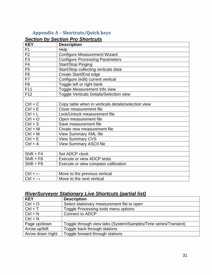
Appendix A – Shortcuts/Quick keys Section by Section Pro Shortcuts KEY Description F1 Help F2 Configure Measurement Wizard F3 Configure Processing Parameters F4 Start/Stop Pinging F5 Start/Stop collecting verticals data F6 Create Start/End edge F7 Configure (edit) current vertical F8 Toggle left or right bank F11 Toggle Measurement Info view F12 Toggle Verticals Details/Selection view Ctrl + C Copy table when in verticals details/selection view Ctrl + E Close measurement file Ctrl + L Lock/Unlock measurement file Ctrl + O Open measurement file Ctrl + S Save measurement file Ctrl + W Create new measurement file Ctrl + M View Summary XML file Ctrl + E View Summary CVS Ctrl + A View Summary ASCII file Shift + F4 Set ADCP clock Shift + F8 Execute or view ADCP tests Shift + F9 Execute or view compass calibration Ctrl + ← Move to the previous vertical Ctrl + → Move to the next vertical RiverSurveyor Stationary Live Shortcuts (partial list) KEY Description Ctrl + O Select stationary measurement file to open Ctrl + T Toggle Processing tools menu options Ctrl + N Connect to ADCP Ctrl + N Page up/down Toggle through view tabs (System/Samples/Time series/Transect) Arrow up/left Toggle back through stations Arrow down /right Toggle forward through stations

32

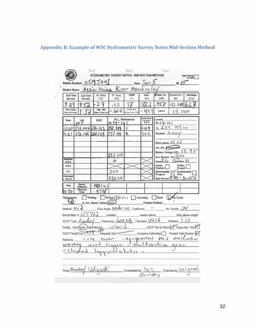
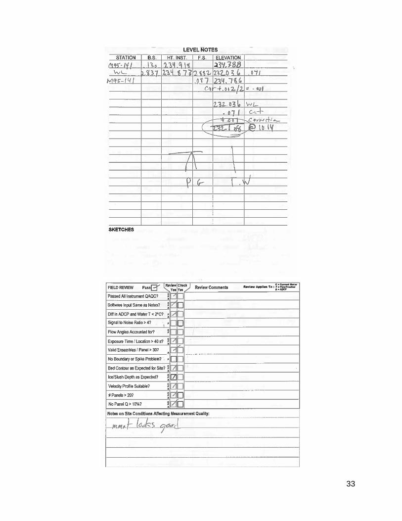
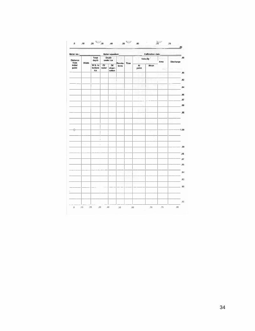
Appendix B: Example of WSC Hydrometric Survey Notes Mid-Section Method

35

Appendix C – Water Survey of Canada Under Ice Hardware System – Mark 2

The Water Survey of Canada Under Ice Hardware system was designed to provide a complete suite of deployment options for all under ice velocity measurement sensors currently available for use by Water Survey of Canada. This integrated system is designed around the WSC standard winter rod system that has been the long standing deployment base for the Price current meter.

This system continues to allow for deployment of the Price current meter but also includes mounts and adapters for use of;

1. FlowTracker ADV

2. StreamPro ADCP

3. RiverRay ADCP

4. S5/M9 ADCP

All new components and hardware are made of aluminum and stainless steel (non-ferrous/ non-magnetic material). Replacement connectors or welded repairs must also be non-ferrous.

Along with the adaptive tools for velocity measurement, the under ice hardware system incorporates improvements to ensure proper orientation of profiling sensors during the velocity measurement process. This includes:

• An orientation line is machined into the surface of the aluminum winter rod over the full length of all rod sections that ensures accurate upstream/downstream orientation/alignment of ADCP sensors. The rod sections are keyed and matched by a coloured “dot” key as part of the overall kit design to ensure correct orientation/alignment is maintained. Although the Price Current Meter and the FlowTracker can easily be deployed with this system, use of the machined surface for orientation does not necessarily apply to sensors that are threaded on to the adaptor. Extra care should be exercised to ensure proper instrument orientation when using either the FlowTracker or the Price Current Meter with this system.

• A new orientation tool that attaches to the machined surface of the winter rod provides a visual aid for ensuring correct alignment along the cross section. Also included is an integrated fish eye bubble for maintaining vertical orientation during measurement.

• As of 2014, an offset bracket has been made available for the RiverRay and M9/S5 mounting kits so they can be deployed at a consistent 10cm distance from the underside of the ice. These are intended to simplify and speed up deployment in slush-free conditions. The RiverRay and M9/S5 brackets are designed to be held up under the ice on the downstream side of the hole so the RiverRay bracket is in-line with Beam 3 and the M9/S5 bracket is opposite the connecter.

36

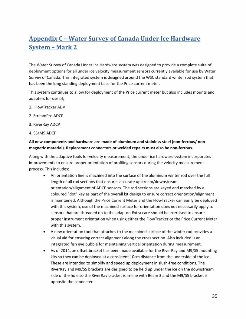
1. Rod System

• The rod system is a modification of the standard WSC winter rod set and includes three (3) one (1) meter upper sections and one (1) lower section, all with machined orientation lines (Figure 23). The orientation line is specific to each rod set. The rod sections all use coloured dots to ensure proper alignment of the orientation line during use (Figures 25-28).

Figure 23 - Keyed winter rod set

Figure 24 - Base section with threaded meter mount.

Figure 25 - First section single "dot" key.

37

Figure 26 - Second section double "dot" key.

Figure 27 - Third section triple "dot" key

Figure 28 - First section and orientation line connected

38

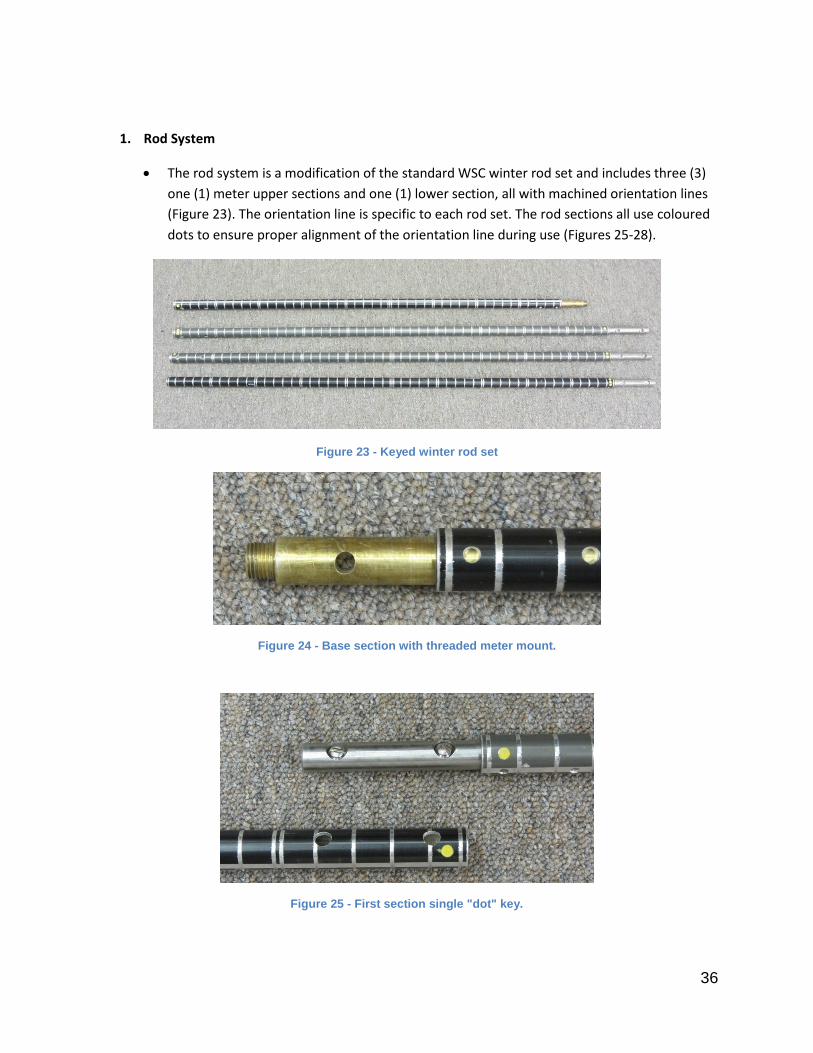
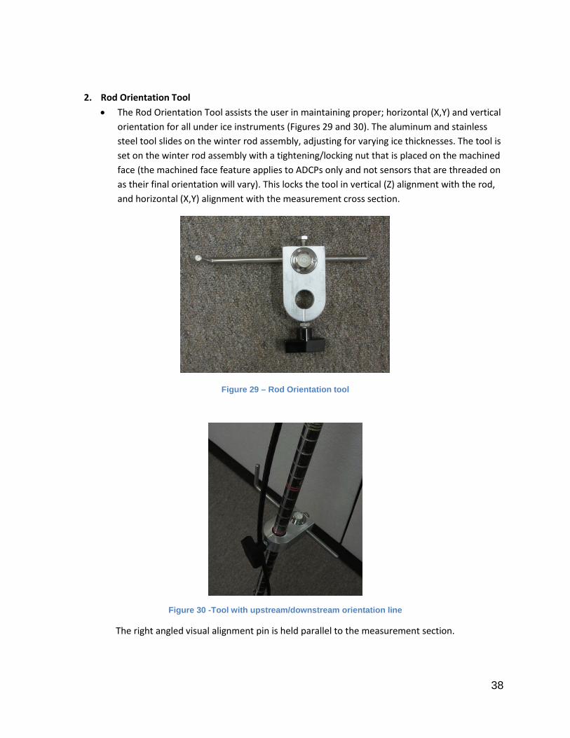
2. Rod Orientation Tool • The Rod Orientation Tool assists the user in maintaining proper; horizontal (X,Y) and vertical

orientation for all under ice instruments (Figures 29 and 30). The aluminum and stainless steel tool slides on the winter rod assembly, adjusting for varying ice thicknesses. The tool is set on the winter rod assembly with a tightening/locking nut that is placed on the machined face (the machined face feature applies to ADCPs only and not sensors that are threaded on as their final orientation will vary). This locks the tool in vertical (Z) alignment with the rod, and horizontal (X,Y) alignment with the measurement cross section.

Figure 29 – Rod Orientation tool

Figure 30 -Tool with upstream/downstream orientation line

The right angled visual alignment pin is held parallel to the measurement section.

39

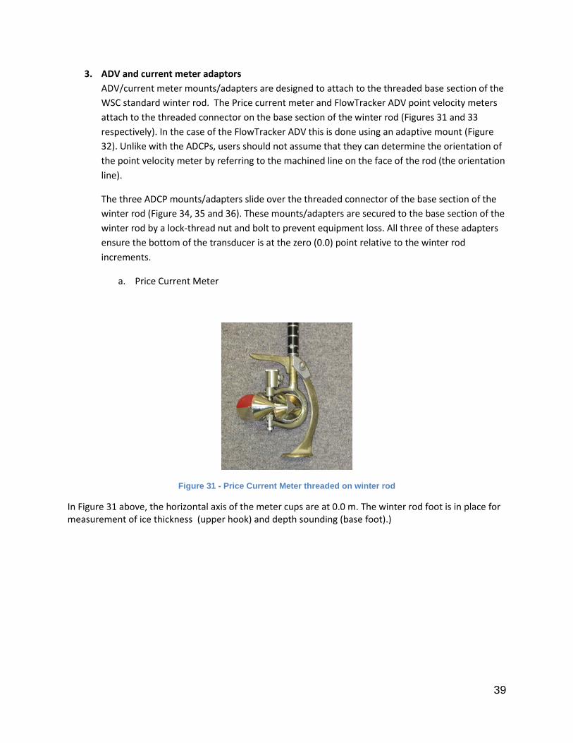
3. ADV and current meter adaptors ADV/current meter mounts/adapters are designed to attach to the threaded base section of the WSC standard winter rod. The Price current meter and FlowTracker ADV point velocity meters attach to the threaded connector on the base section of the winter rod (Figures 31 and 33 respectively). In the case of the FlowTracker ADV this is done using an adaptive mount (Figure 32). Unlike with the ADCPs, users should not assume that they can determine the orientation of the point velocity meter by referring to the machined line on the face of the rod (the orientation line).

The three ADCP mounts/adapters slide over the threaded connector of the base section of the winter rod (Figure 34, 35 and 36). These mounts/adapters are secured to the base section of the winter rod by a lock-thread nut and bolt to prevent equipment loss. All three of these adapters ensure the bottom of the transducer is at the zero (0.0) point relative to the winter rod increments.

a. Price Current Meter

Figure 31 - Price Current Meter threaded on winter rod

In Figure 31 above, the horizontal axis of the meter cups are at 0.0 m. The winter rod foot is in place for measurement of ice thickness (upper hook) and depth sounding (base foot).)

40

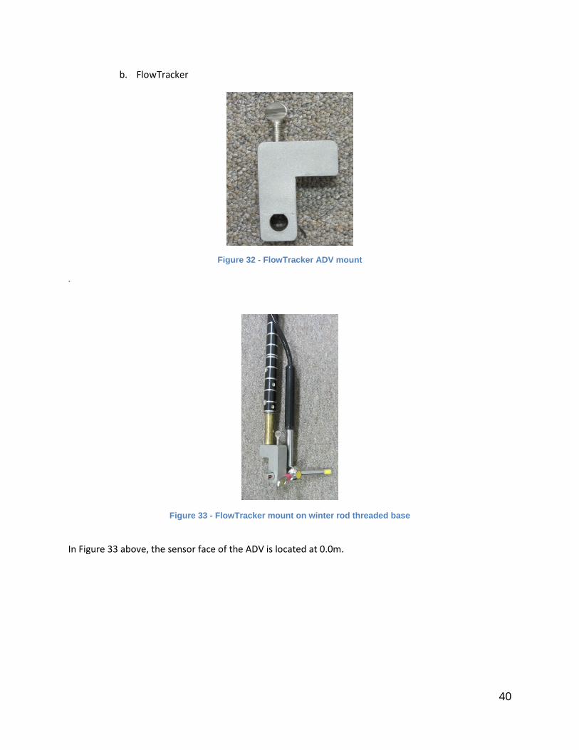
b. FlowTracker

Figure 32 - FlowTracker ADV mount

.

Figure 33 - FlowTracker mount on winter rod threaded base

In Figure 33 above, the sensor face of the ADV is located at 0.0m.

41

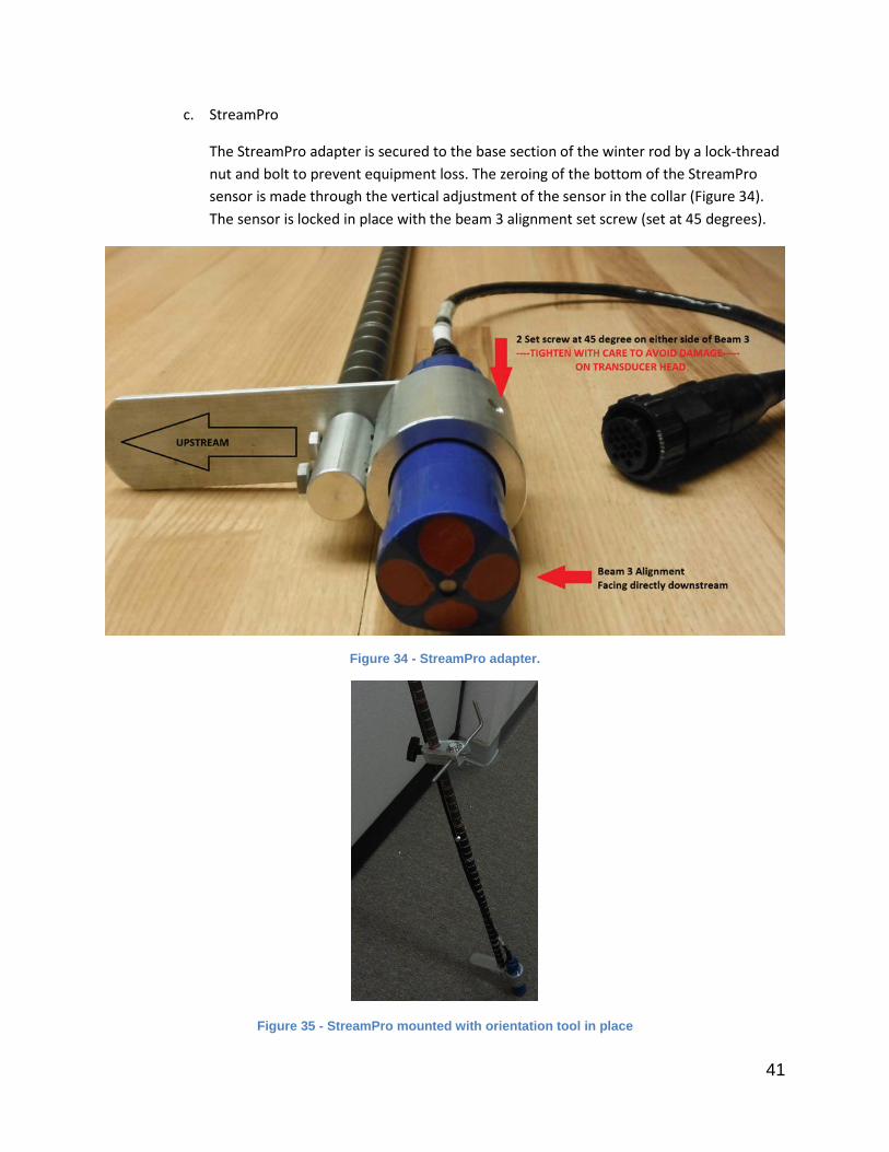
c. StreamPro

The StreamPro adapter is secured to the base section of the winter rod by a lock-thread nut and bolt to prevent equipment loss. The zeroing of the bottom of the StreamPro sensor is made through the vertical adjustment of the sensor in the collar (Figure 34). The sensor is locked in place with the beam 3 alignment set screw (set at 45 degrees).

Figure 34 - StreamPro adapter.

Figure 35 - StreamPro mounted with orientation tool in place

42

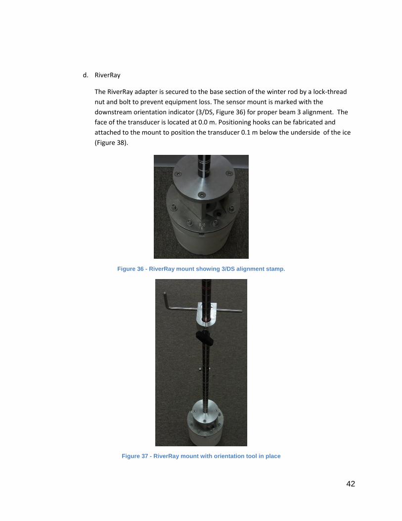
d. RiverRay

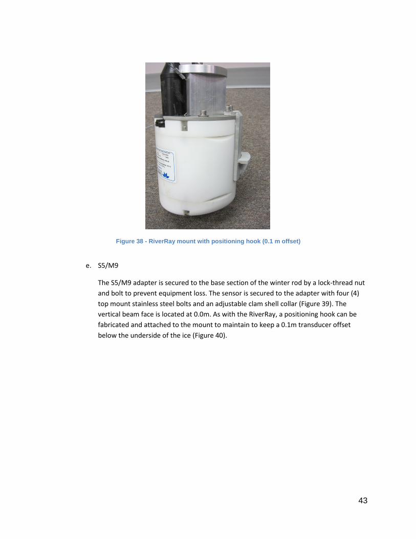
The RiverRay adapter is secured to the base section of the winter rod by a lock-thread nut and bolt to prevent equipment loss. The sensor mount is marked with the downstream orientation indicator (3/DS, Figure 36) for proper beam 3 alignment. The face of the transducer is located at 0.0 m. Positioning hooks can be fabricated and attached to the mount to position the transducer 0.1 m below the underside of the ice (Figure 38).

Figure 36 - RiverRay mount showing 3/DS alignment stamp.

Figure 37 - RiverRay mount with orientation tool in place

43

Figure 38 - RiverRay mount with positioning hook (0.1 m offset)

e. S5/M9

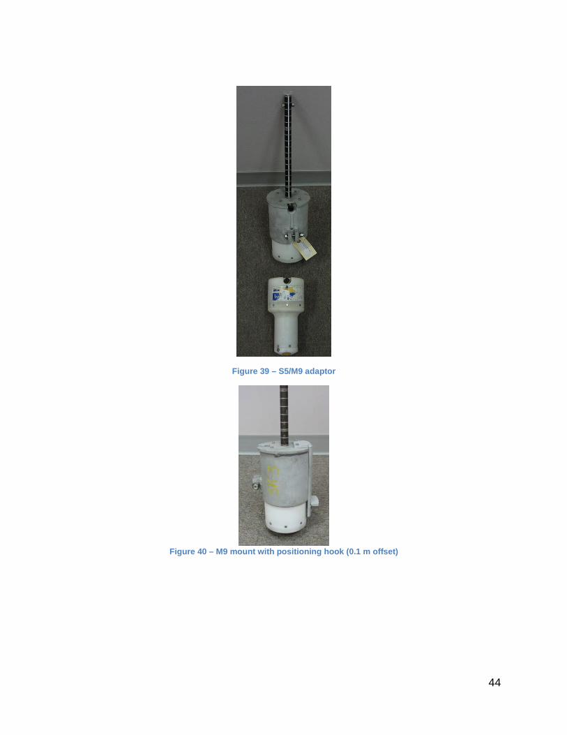
The S5/M9 adapter is secured to the base section of the winter rod by a lock-thread nut and bolt to prevent equipment loss. The sensor is secured to the adapter with four (4) top mount stainless steel bolts and an adjustable clam shell collar (Figure 39). The vertical beam face is located at 0.0m. As with the RiverRay, a positioning hook can be fabricated and attached to the mount to maintain to keep a 0.1m transducer offset below the underside of the ice (Figure 40).

44

Figure 39 – S5/M9 adaptor

Figure 40 – M9 mount with positioning hook (0.1 m offset)

45

4. Transport Case

The transport case (Figure 41) is an integrated system and as such all components must be maintained as part of each kit. A Pelican transport case is supplied to ensure the maintenance of all matched/keyed components.

Figure 41 - Standard transport case configuration for all adapters.

Standard Operating Procedures for under ice ... - USGS · discharge measurements using ADCPs ....

Documents

Transcript of Standard Operating Procedures for under ice ... - USGS · discharge measurements using ADCPs ....