STANDARD OPERATING PROCEDURES FOR FIELD SAMPLERS …denr.sd.gov/dfta/wp/Vol1SOP.pdf · standard...
175
STANDARD OPERATING PROCEDURES FOR FIELD SAMPLERS VOLUME I TRIBUTARY AND IN-LAKE SAMPLING TECHNIQUES STATE OF SOUTH DAKOTA DEPARTMENT OF ENVIRONMENT AND NATURAL RESOURCES WATER RESOURCES ASSISTANCE PROGRAM STEVEN M. PIRNER, SECRETARY FEBRUARY 2005
Transcript of STANDARD OPERATING PROCEDURES FOR FIELD SAMPLERS …denr.sd.gov/dfta/wp/Vol1SOP.pdf · standard...
STANDARD OPERATING PROCEDURES FOR FIELD SAMPLERS
VOLUME I
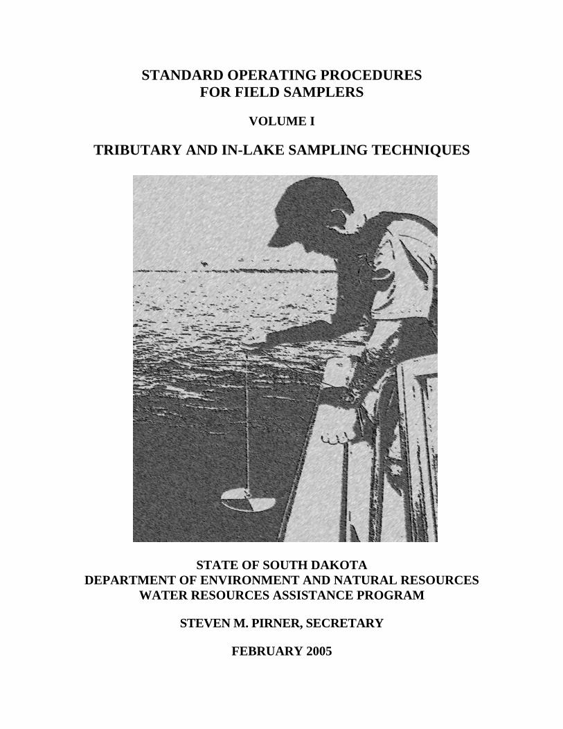
TRIBUTARY AND IN-LAKE SAMPLING TECHNIQUES
STATE OF SOUTH DAKOTA
DEPARTMENT OF ENVIRONMENT AND NATURAL RESOURCES WATER RESOURCES ASSISTANCE PROGRAM
STEVEN M. PIRNER, SECRETARY
FEBRUARY 2005


STANDARD OPERATING PROCEDURES FOR FIELD SAMPLERS
VOLUME I
TRIBUTARY AND IN-LAKE SAMPLING TECHNIQUES
Prepared by
Watershed Assessment Team
STATE OF SOUTH DAKOTA DEPARTMENT OF ENVIRONMENT AND NATURAL RESOURCES
WATER RESOURCES ASSISTANCE PROGRAM
STEVEN M. PIRNER, SECRETARY
Revision 5.2.2
February 2005

i
TABLE OF CONTENTS
1.0 INTRODUCTION AND BACKGROUND....................................................................... 1.0-1
2.0 WATERSHED RESOURCES ASSISTANCE PROGRAM DESCRIPTION.......................... 2.0-1
3.0 STUDY AREA DESCRIPTION ....................................................................................... 3.0-1 Regional Characteristics ............................................................................................... 3.0-1 Ecoregions .................................................................................................................... 3.0-3
4.0 PRE-SAMPLING PROCEDURES ................................................................................... 4.0-1
5.0 DOCUMENTATION AND REPORTING ....................................................................... 5.0-1 Documentation.............................................................................................................. 5.0-1
Logbook ............................................................................................................ 5.0-1 Reporting ...................................................................................................................... 5.0-2
6.0 INSTRUMENT CALIBRATION...................................................................................... 6.0-1 A. Dissolved Oxygen Meter - Model 51B, air calibration.......................................... 6.0-1 B. pH Meter ................................................................................................................. 6.0-5 C. Conductivity Meter ................................................................................................. 6.0-8
Solution-Calibrated Conductivity Meter. ......................................................... 6.0-8 Red Line-Calibrated Conductivity Meter. ........................................................ 6.0-8
D. Turbidity Meter ....................................................................................................... 6.0-8 HF Scientific, Model DRT-15 .......................................................................... 6.0-8
E. Flow Meter .............................................................................................................. 6.0-9 Marsh-McBirney, Model 201. .......................................................................... 6.0-9 Aquacalc 5000. ................................................................................................. 6.0-9
F. CALIBRATION PROCEDURES for YSI Multi Meters ...................................... 6.0-10 Temperature .................................................................................................... 6.0-11 Depth and Level.............................................................................................. 6.0-11 Dissolved Oxygen (DO) ................................................................................. 6.0-12 Sampling Applications.................................................................................... 6.0-14 Conductivity.................................................................................................... 6.0-15 pH 2-POINT.................................................................................................... 6.0-17 Turbidity 2-Point............................................................................................. 6.0-18 Chlorophyll a 1-Point ..................................................................................... 6.0-18 YSI Calibration Reset Procedure.................................................................... 6.0-19 YSI Data Download Procedure....................................................................... 6.0-21

ii
TABLE OF CONTENTS (Continued)
G. Stage Recorders and Data Loggers ....................................................................... 6.0-21
ISCO 4230 Flow Meter................................................................................... 6.0-22 ISCO GLS Sampler......................................................................................... 6.0-23 ISCO 6700 Auto Sampler with 730 ................................................................ 6.0-24 Downloading ISCO 4230 and 6700 Samplers ................................................ 6.0-23 Downloading Rapid Transfer Device (RTD).................................................. 6.0-24 OTT Thalimedes ............................................................................................. 6.0-25 OTT Nimbus ................................................................................................... 6.0-27 Stevens Type F Stage Recorders .................................................................... 6.0-32 R2 Data Logger Setup, Calibration, and Downloading Method..................... 6.0-33
7.0 CHAIN OF CUSTODY..................................................................................................... 7.0-1 Documentation.............................................................................................................. 7.0-1 Field Custody................................................................................................................ 7.0-1 Transfer of Custody and Shipment ............................................................................... 7.0-2
8.0 QUALITY ASSURANCE ................................................................................................. 8.0-1 General Information and Handling Procedures ............................................................ 8.0-1 QA/QC Sampling.......................................................................................................... 8.0-2
Replicates.......................................................................................................... 8.0-2 Field Blanks ...................................................................................................... 8.0-3
Precision and Accuracy ................................................................................................ 8.0-3 Precision............................................................................................................ 8.0-3 Accuracy ........................................................................................................... 8.0-4
Preventive Maintenance................................................................................................ 8.0-8
9.0 LABORATORY ANALYTICAL METHODS ................................................................. 9.0-1 Analytical Procedures ................................................................................................... 9.0-1
10.0 SAMPLE CONTAINERS, PRESERVATION AND HOLDING TIMES.................... 10.0-1 11.0 DECONTAMINATION OF SAMPLE CONTAINERS AND SAMPLING
EQUIPMENT ............................................................................................................. 11.0-1
TRIBUTARY SAMPLING TECHNIQUES (Yellow Index Section)
12.0 SAMPLING PROCEDURES FOR TRIBUTARY SAMPLING .................................. 12.0-1 Field Observations ...................................................................................................... 12.0-1

iii
TABLE OF CONTENTS (Continued)
Field Analyses............................................................................................................. 12.0-2 YSI Multi Parameter Meter (650 MDS with Sonde) Method ........................ 12.0-2 Dissolved Oxygen Meter (YSI Model 51B) ................................................... 12.0-2 pH-Electrode Method ..................................................................................... 12.0-3 Temperature .................................................................................................... 12.0-3 Total Depth ..................................................................................................... 12.0-3 Flow (Marsh-McBirney)................................................................................. 12.0-4 Flow (AquaCalc 5000) .................................................................................... 12.0-5 Stage Recording/Data Logging....................................................................... 12.0-7
Sample Collection....................................................................................................... 12.0-7 Grab Sampling ................................................................................................ 12.0-8 Composite Sampling..................................................................................... 12.0-13 Suspended Sediment Sampler....................................................................... 12.0-13 Suspended Sediment Sampling Procedure.................................................... 12.0-15
Chlorophyll a Sampling............................................................................................ 12.0-17 Procedure for Tributary Chlorophyll a Sampling......................................... 12.0-17
Shipping the Sample ................................................................................................. 12.0-20 General Samples ........................................................................................... 12.0-20 Chain-of-Custody Samples ........................................................................... 12.0-20
13.0. WATERSHED MODELING........................................................................................ 13.0-1 Agricultural Non-Point Source (AGNPS) and Annualized Agricultural Non-Point
Source (AnnAGNPS) Watershed Models....................................................... 13.0-1 Pacific Southwest Interagency Committee (PSIAC) Sediment Evaluation Method .. 13.0-1 FLUX Model............................................................................................................... 13.0-2
IN-LAKE SAMPLING TECHNIQUES
(Blue Index Section)
14.0 IN-LAKE SAMPLING PROCEDURES.................................................................... 14.0-1 Field Observations ...................................................................................................... 14.0-1 Field Analyses............................................................................................................. 14.0-2
YSI Multi Parameter Meter (650 MDS with Sonde) Method ........................ 14.0-2 Dissolved Oxygen Meter (YSI Model 51B) ................................................... 14.0-3 Temperature .................................................................................................... 14.0-4 Dissolved Oxygen/Temperature Profiles........................................................ 14.0-4 pH-Electrode Method ..................................................................................... 14.0-4 Secchi Depth ................................................................................................... 14.0-5 Total Depth ..................................................................................................... 14.0-5

iv
TABLE OF CONTENTS (Continued) In-lake Water Sampling Method (Van Dorn-type sampler) ....................................... 14.0-5
Sampler Setup Procedure................................................................................ 14.0-6 In-lake Sample Collection .......................................................................................... 14.0-7
Grab Sampling ................................................................................................ 14.0-8 Collecting a Sample (without the use of a Van Dorn-type sampler) .............. 14.0-8 Collecting a Sample (with the use of a Van Dorn-type sampler) ................. 14.0-14 Composite Sampling..................................................................................... 14.0-17 Collecting the Composite Sample................................................................. 14.0-17
Chlorophyll a Sampling............................................................................................ 14.0-18 Shipping the Sample ................................................................................................. 14.0-20
General Samples ........................................................................................... 14.0-20 Chain-of-Custody Samples ........................................................................... 14.0-20
15.0. IN-LAKE MODELING.............................................................................................. 15.0-1 BATHTUB Model ...................................................................................................... 15.0-1 PROFILE Model......................................................................................................... 15.0-1
SPECIAL SAMPLING TECHNIQUES (Green Index Section)
16.0. CAFFEINE SAMPLING............................................................................................ 16.0-1 Purpose........................................................................................................................ 16.0-1 Materials ..................................................................................................................... 16.0-1 Sample Collection....................................................................................................... 16.0-1
Grab Sampling (tributary or in-lake) .............................................................. 16.0-2 Composite Sampling (tributary and in-lake) .................................................. 16.0-3
Shipping the Sample ................................................................................................... 16.0-5 General Samples ............................................................................................. 16.0-5 Chain-of-Custody Samples ............................................................................. 16.0-5
QA/QC Samples.......................................................................................................... 16.0-6
17.0. METAL SAMPLING ................................................................................................. 17.0-1 Sample Collection....................................................................................................... 17.0-1 Sampling Procedures .................................................................................................. 17.0-1
Tributary sampling.......................................................................................... 17.0-1 Lake sampling................................................................................................. 17.0-2
Shipping the Sample ................................................................................................... 17.0-3 General Samples ............................................................................................. 17.0-3 Chain-of-Custody Samples ............................................................................. 17.0-3

v
TABLE OF CONTENTS (Continued) QA/QC Samples.......................................................................................................... 17.0-4
18.0. ELUTRIATE SAMPLING (Lake Sediment Sampling) ............................................. 18.0-1 Purpose........................................................................................................................ 18.0-1 Materials ..................................................................................................................... 18.0-1 Procedure .................................................................................................................... 18.0-2 Sampling Site Procedures ........................................................................................... 18.0-2 Grab Sampling ............................................................................................................ 18.0-2 Composite Sampling................................................................................................... 18.0-4 Shipping the Sample ................................................................................................... 18.0-6
General Samples ............................................................................................. 18.0-6 Chain-of-Custody Samples ............................................................................. 18.0-6
Quality Control (Field) ............................................................................................... 18.0-7 Quality Control (Lab) ................................................................................................. 18.0-8
19.0 DISCRETE GRAB SAMPLES FOR UPSTREAM AND DOWNSTREAM SAMPLING ................................................................................................................. 19.0-1 Site Location ............................................................................................................... 19.0-1 Sample Collection....................................................................................................... 19.0-2 Shipping the Samples.................................................................................................. 19.0-2
General Samples ............................................................................................. 19.0-2 Chain-of-Custody Samples ............................................................................. 19.0-2
20.0 PESTICIDE SAMPLING ........................................................................................... 20.0-1 Purpose........................................................................................................................ 20.0-1 Materials ..................................................................................................................... 20.0-1 Procedure .................................................................................................................... 20.0-1 Sampling Procedures .................................................................................................. 20.0-2
Tributary Procedures....................................................................................... 20.0-2 In-lake Procedures .......................................................................................... 20.0-3
Grab Sampling (without a sampling device) ...................................... 20.0-3 Grab Sampling (with a sampling device) ........................................... 20.0-4
Shipping Samples........................................................................................................ 20.0-5 General Samples ............................................................................................. 20.0-5 Chain-of-Custody Samples ............................................................................. 20.0-6
Quality Control (Field) ............................................................................................... 20.0-7 Quality Control (Lab) ................................................................................................. 20.0-7

vi
TABLE OF CONTENTS (Continued)
21.0 RIBOTYPING SAMPLING....................................................................................... 21.0-1
22.0. REFERENCES CITED............................................................................................... 22.0-1
vii
LIST OF FIGURES
Figure 3.0.1. South Dakota Level III Ecoregions .................................................................... 3.0-4 Figure 6.0.1. Dissolved oxygen probe membrane replacement procedure.............................. 6.0-3 Figure 6.0.2. Oakton pH meter. ............................................................................................... 6.0-7 Figure 12.0.1. Wading rod for the Marsh-McBirney flowmeter ........................................... 12.0-5 Figure 12.0.2. Fill diagram and presevative for typical wrap tributary sampling suite......... 12.0-9 Figure 12.0.3. Nalgene Filter Holder with Receiver and Vacuum Pump.. .......................... 12.0-12 Figure 12.0.4. General use of the suspended sediment sampler used by SD WRAP.. ........ 12.0-13 Figure 14.0.1. Van Dorn-type sampler.. ................................................................................ 14.0-5 Figure 14.0.2. Fill diagram and preservative for typical SD WRAP in-lake sampling suite.14.0-9 Figure 14.0.3. Nalgene Filter Holder with Receiver and Vacuum Pump.. .......................... 14.0-13

viii
LIST OF TABLES Table 6.0.1. YSI calibration constants................................................................................... 6.0-20 Table 8.0.1. South Dakota Department of Health precision and accuracy statement.............. 8.0-5 Table 9.0.1. Methods and references for physical and chemical parameters.. ........................ 9.0-1 Table 10.0.1. Recommended containers, preservation techniques and holding times for
inorganics... ...................................................................................................... 10.0-1 Table 10.0.2. Recommended containers, preservation techniques and holding times for
organics... ......................................................................................................... 10.0-3

ix
APPENDICES
Appendix A South Dakota Water Resources Assistance Programs datasheets

Section 1.0 Page 1 of 1 Revision 5.2.2
1.0 INTRODUCTION AND BACKGROUND
The lakes and rivers of South Dakota provide a basic natural resource, recreational in nature, of utmost importance to the economy of the state and quality of life for its 754,844 residents (Census 2000). Approximately 800 lakes, ranging in size from prairie potholes to the Missouri River mainstem reservoirs, are readily available for public use. Five hundred seventy-three state lakes have been recognized as significant waterbodies, specifically categorized by the South Dakota Department of Environment and Natural Resources as to their assigned beneficial uses.
The great majority of state lakes are relatively small and naturally shallow, often situated on sizeable watersheds comprised of nutrient-rich glacial soils. Consequently, both natural and cultural eutrophication are likely to proceed at much higher rates than in larger, deep lakes located in less-fertile surroundings in other parts of the country. Physical and biological changes, made manifest only after decades in larger bodies of water, are often visible in many South Dakota lakes within a few years.
Agricultural practices in South Dakota, as elsewhere, have intensified over past decades and are major contributors to cultural eutrophication via nutrient loss and sedimentation. Much of this process can be prevented or impeded by proper land and watershed management procedures that are incorporated into the South Dakota Water Resources Assistance Program.
One of the main objectives of the Water Resources Assistance Program is to assess the water quality of lakes and their watersheds. Assessments are accomplished by describing the current conditions in impacted watersheds, tracking trends in water quality, determining sources of lake and stream degradation, targeting these sources, and setting reachable, obtainable goals for water quality improvement. Chemical, physical, and biological characteristics of the lakes and their tributaries are assessed. The trophic status of each lake is also described. Obtaining quality data is essential to achieving these goals.
Of vital importance in the early stages of a watershed assessment project is the compilation of baseline data and the establishment of baseline conditions that can later be compared with data collected after lake and stream protection/restoration measures have been carried out. Only in this way can changes in lake or stream water quality be reliably ascribed either to natural variation or to the effects of mitigation or watershed restoration efforts.
It is imperative that proper field procedures be followed during sample collection and that samples are collected in a consistent manner. Standard Operating Procedures (SOP) activities will ensure accurate, precise, and representative lake and tributary data as well as continuity in methodology between projects. This document describes the standard operating procedures to be used by Watershed Resources Assistance Program personnel.

Section 2.0 Page 1 of 2 Revision 5.2.2
2.0 WATERSHED RESOURCES ASSISTANCE PROGRAM DESCRIPTION
The South Dakota Water Resources Assistance Program (SDWRAP) is designed as a two-phased effort to 1) identify sources of pollution and determine alternative restoration methods, and 2) control the sources of pollution and restore the quality of state lakes and streams. The program is typically a state and local endeavor, with financial and technical assistance from federal agencies used whenever possible.
The watershed assessment stage of the program encompasses a series of procedures to assess the current condition of selected water bodies. Included in this phase are water quality, water quantity and watershed data collection. Generally, the local project sponsors are responsible for collecting the data using existing local resources or in combination with Section 319(h) (supplemental grant) funding. SDWRAP provides equipment, training and technical assistance to the project sponsor. Following the collection of sufficient data, SDWRAP conducts an evaluation of the data and prepares a report. This assessment summarizes baseline information, identifies sources of pollution, describes alternative pollution control and restoration methodologies, outlines implementation costs and details SDWRAP recommendations. The state provides these services using Section 319(h) funding and local matching funds.
Prior to the implementation of specific pollution control and restoration alternatives, the local project sponsor develops a work plan for in-lake and watershed restoration based on recommendations from the assessment. Technical assistance for this process is provided by SDWRAP. This plan is then submitted to the State Water Plan administrators for consideration. If the plan is approved, the project sponsors are eligible to apply for appropriate state funding. The primary funding sources used by the sponsors are the State Consolidated Water Facilities Construction Fund, Conservation Commission Fund, USDA EQIP funds, the EPA Section 319 (h) Implementation Fund and local funding.
Nonpoint source pollution from agricultural activities is the primary pollution source affecting lakes and streams in South Dakota. The methods used to control this source are selected on a case-by-case basis. Selection is based on evaluation of individual watersheds using the Annualized Agricultural Nonpoint Source Model, AnnAGNPS (USDA-ARS, 2000). The model delineates critical areas within the watershed and is then used to predict which control methods would be most effective.

Section 2.0 Page 2 of 2 Revision 5.2.2
Following the AnnAGNPS evaluation, coordination with state and federal agricultural agencies is solicited to verify the nature of the identified critical cells and the selected control methods. For those areas targeted as critical, the owners/operators are contacted to request their voluntary participation in the control program. There are no provisions for forcing compliance to correct identified problem areas. Best Management Practices (BMPs) used in a watershed restoration plan may include, but are not limited to, mechanical and managerial, large and small sediment control structures, shoreline erosion control, and the installation of Animal Waste Management Systems (AWMS). In those few instances where point source pollution may be a problem, the best available technology is applied to correct the problem.
In conjunction with the development of watershed pollution control alternatives, the assessment data evaluation may also provide recommendations for stream and lake restoration alternatives. Again, the recommendations are made on a case-by-case basis with input from all concerned organizations. Funding for implementation is made available primarily though the State Consolidated Water Facilities Construction Fund, the EPA 319, USDA EQIP, Nonpoint Source Program and local funding.
In-lake recommendations may include, but are not limited to, natural flushing (after reducing or eliminating sources of pollution), sediment removal, in-lake phosphorus control, weed harvesting, chemical weed control and some preliminary attempts at biomanipulation. The recommendations for in-lake BMPs are implemented after or in conjunction with watershed BMPs.
A unique element of the lake restoration program in South Dakota is the availability of hydraulic dredges in the state. Because sedimentation has been identified as a major problem in South Dakota lakes, these dredges provide a viable restoration alternative for silted lakes. The process for assignment of dredges to specific lakes is based on the recommendations of individual Watershed Assessment Study reports, the availability of equipment, and funding elements.

Section 3.0 Page 1 of 4 Revision 5.2.2
3.0 STUDY AREA DESCRIPTION
A. Regional Characteristics
South Dakota is a rural, agricultural state with a surface area of 77,047 square miles. Rolling plains are the main topographic feature of this northern prairie state. The most visible geographic forms in the state are the Missouri River, which divides the state into 'East River' and 'West River' areas, and the Black Hills - an isolated area of granitic uplift in the far west. The maximum elevation of the state is 2,210 meters (7,242 feet) at Harney Peak in the Black Hills. The lowest elevation, 294 meters (965 feet) is near Big Stone City in the bed of Big Stone Lake.
The unglaciated West River mixed-and short-grass prairie of South Dakota has few natural lakes, but a number of man-made lakes and numerous small farm ponds are found in the western prairie region of the state. Three large Missouri River mainstem reservoirs form the eastern boundary of the West River prairie. The majority of lakes within the Black Hills are also impoundments.
The particular geology of an area exerts considerable influence on both the surface and ground water quality. Rothrock (1943) and Flint (1955) recognized 12 major physical regions within state boundaries. As a result of this geologic diversity, the water quality of the state is highly variable. The water quality of eastern South Dakota (Prairie Coteau) is indicative of the types of glacial drift deposited at various localities, and the Dakota Sandstone aquifer (Nickum, 1969).
South Dakota has a sub-humid to semiarid climate subject to periods of drought at roughly 20-year intervals. Due to the shallow nature of the lake basins formed by glaciers in the region, average water depth of eastern state lakes is less than eight feet. During a prolonged drought, many lakes may dry up completely, while others are reduced to very low water levels with attendant high salt concentration.
For this reason, most of the prairie lakes of eastern South Dakota can be classified as warmwater semi-permanent. These lakes respond quickly to changes in annual rainfall and the underlying water table with fluctuations in lake water levels and water quality. The majority of state lakes tend to be turbid and well-supplied with dissolved salts, nutrients, and organic matter mostly by runoff from agricultural and domestic sources. The shallowness of the lakes, together with the mixing action exerted by strong summer winds, prevents continuous thermal stratification in all but a few cases.

Section 3.0 Page 2 of 4 Revision 5.2.2
Intensive agricultural practices have contributed greatly to the cultural process of lake eutrophication via soil loss and sedimentation. Fortunately, much of the cultural process can be prevented or impeded by the planned and timely application of watershed and lake preservation and restoration measures adopted by SD WRAP.
Approximately one hundred twenty-five lakes and reservoirs are currently being monitored statewide to assess their water quality. The present goals of this sampling effort, TMDL assessments and SD WRAP are as follows:
1. Establish baseline water quality information, particularly for sediment and nutrients.
2. Enter lake and tributary water quality data into the USEPA STORET computer system and the SD WRAP Water Quality Database.
3. Assess the trophic status of the lakes. 4. Determine whether the assessed lakes are meeting assigned water quality
beneficial use criteria. 5. Document long-term trends in water quality. 6. Determine attainable goals and targets for impaired waterbodies.
South Dakota has a total of 10,298 miles of rivers and major streams. Major or significant streams in this context are waters that have been assigned aquatic life use support in addition to the beneficial uses of fish and wildlife propagation, recreation, stockwatering and irrigation. This definition includes primary tributaries and, less frequently, sub-tributaries of most state rivers and larger perennial streams. In a few cases, lower order tributaries may be included, for example in the Black Hills area, which has a relatively large number of permanent streams. If all existing and mostly waterless stream channels and gullies are to be included as state waters, the great majority of which serve only to carry snowmelt or stormwater runoff for a week or two during an average year, total stream mileage within South Dakota would exceed the above quoted figure by at least ten times. Intensive agricultural and cultural practices have contributed greatly to the stream eutrophication via nutrient runoff, soil loss and sedimentation. Many of these impairments can be attributed largely to high levels of total suspended solids (TSS) present in many of the monitored streams. Fortunately, much of the agricultural and cultural process can be prevented or impeded by the planned and timely application of watershed and lake preservation and restoration measures adopted by SD WRAP.
Section 3.0 Page 3 of 4 Revision 5.2.2
B. Ecoregions
1. Due to differences in geography, there are marked variations among the eight Level III ecoregions in South Dakota (Figure 3.0.1). The Black Hills are located in the Middle Rockies ecoregion. The Northwestern Great Plains ecoregion includes most of the South Dakota prairie west of the Missouri River. Also situated in southwestern South Dakota, along the Pine Ridge Indian reservation, is the Western High Plains ecoregion. There is a small area of the Nebraska Sandhills ecoregion, which encroaches on the southern border of South Dakota in Shannon, Bennett, and Todd counties. The Northwestern Glaciated Plain ecoregion covers the Missouri River plateau east of the Missouri River. There is a small area of this ecoregion reaching into the West River area near the Nebraska border. The Northern Glaciated Plains ecoregion covers the majority of eastern South Dakota from the James River valley to the eastern border. Only two smaller Level III ecoregion areas are found in the rest of the state. The extreme northeastern corner of the state is touched by the Lake Agassiz Plain, which extends north into the Red River Valley. Also, patches of the Western Corn Belt Plains ecoregion encroach into South Dakota from the borders of southwest Minnesota and northwest Iowa.
2. By definition, these different ecoregions support different compositions of biota. By sampling the biota we should be able to find marked differences in the biological communities. This SOP will lay out step by step instructions for the collection of algae and macroinvertebrates, including, but not limited to, site selection, habitat assessment, land use and chemical water sampling. The SOP will also describe procedures for laboratory analysis and data management.

Section 3.0 Page 4 of 4 Revision 5.2.2
30
15 0
120 km60
60 mi
SCALE 1:1,500,00030
0
44 Nebraska17 Middle 43 Northwestern Great 47 Western Corn Belt
25 Western High 42 Northwestern Glaciated 46 Northern Glaciated 48 Lake Agassiz
South Dakota Level III Ecoregions
17
25
44
43 42 46
47
48
Figure 3.0.1. South Dakota Level III Ecoregions.

Section 4.0 Page 1 of 1
Revision 5.2.2
4.0 PRE-SAMPLING PROCEDURES
Each field investigation must be evaluated and designed on an individual basis. Common procedures addressed in developing an assessment work plan include the following:
A. Determine the objectives for sampling. B. Review existing information and data on the waterbody under investigation. C. Obtain adequate maps and diagrams to define the study area. D. Conduct field reconnaissance of the proposed study area. E. Develop a list of proposed sampling sites, sampling frequency, and sample analysis. F. Review entire project and insure QA/QC sampling is adequate. G. Arrange schedules, responsibilities, funding and contracts with all agencies,
sponsors and laboratories involved with the study. Coordinate all activities. H. Develop a list of necessary equipment and supplies. I. Check the operation of all equipment prior to field use.
Section 5.0 Page 1 of 2 Revision 5.2.2
5.0 DOCUMENTATION AND REPORTING
A. Documentation A field notebook is REQUIRED to keep track of the sample date and time and the calibration of equipment. Use a write-in-the-rain notebook with bound and numbered pages. Use the same notebook for all project observations and samples. A standard format is not required; however, entries in the field logbook will be legible and include, but not be limited to, the following: 1. Logbook
a. In the front of the logbook, record the types of meters being used, the
meter serial number and the state ID number, if available. b. Record the site or location where the calibration and inspection took
place. c. Record the date and time when the calibration and inspection took
place. d. Record the elevation (mean sea level - MSL) to which the dissolved
oxygen meter was calibrated if air calibration was the method used. e. Record the pH meter reading when the instrument probe was placed
in a known buffer solution during calibration. f. Record the conductivity meter reading for a known calibration
solution (conductance is in µS/cm). g. Recheck the calibration at each site.
a. If the meter drifts between locations, report the drift in the
logbook at the site where it occurred. b. If a meter drifts, recalibrate and record the re-calibration. c. Make notes of any damage to the instrument or difficulty in
operation or calibration.
h. Record all field observations, information, tributary stage data and sample information in the logbook at each site.
i. Air and water temperature. j. Cloud cover, precipitation. k. Number and type of data sheets filled out at each site (i.e. Flow data
sheet) l. REMEMBER!! You cannot put too much information in the
logbook!
Section 5.0 Page 2 of 2 Revision 5.2.2
m. NOTE: Initial or sign and date each day’s entry in the logbook. n. Report any difficulties or malfunctions to the project officer as soon
as possible.
B. Reporting Monthly reporting is REQUIRED for all project coordinators and will encompass but is not limited to: 1. Stage and Flow Data
Monthly stage and flow measurements will be provided to the project officer for data analysis and validation in an Excel spreadsheet format.
2. Chemical Water Quality Data Monthly updates of chemical, biological and field data entered into Access® Storet program or on Excel® spreadsheet format depending on project officer.
3. AnnAGNPS Landuse Data Monthly updates AnnAGNPS data collection as per outlined schedule. Data requirements will be in either Excel® or Arcview® format, depending on project officer.
4. Updated Equipment List Initial equipment list including model and serial numbers and site location will be required at the beginning of each project (Appendix A). Any alterations, problems, maintenance and/or other deficiencies throughout the project with be noted and an updated list will be required as equipment needs and or locations change. The completed and/or modified equipment list will be sent to the equipment officer in Pierre.

Section 6.0 Page 1 of 36 Revision 5.2.2
6.0 INSTRUMENT CALIBRATION
Each field instrument must be calibrated, inspected prior to use, and operated according to manufacturer specifications. If problems with any field instrument are encountered, the user should consult the manufacturer’s manual, the project officer, and/or call the manufacturer. Calibrations and instrument observations must be recorded in a logbook (Section 5.0 - Logbook Procedures) prior to field use.
General calibration procedures and necessary instrument inspections are presented below:
A. Dissolved Oxygen Meter - Model 51B, air calibration
According to the manufacturer, there are three methods used: 1) Winkler-Azide, 2) Saturated Water, and 3) Air Calibration. SD WRAP uses the air calibration method:
1. Make sure cable from the probe is hooked to the meter. 2. If the probe is new or dry (without solution in it), perform the following steps
before continuing: a. Obtain a dissolved oxygen membrane kit. Fill the small dropper
bottle that contains the white crystals with distilled water. These potassium chloride (KCl) crystals, when dissolved in the distilled water, become the electrolyte solution used to bathe the inside of the probe. (If your kit is not new, the electrolyte solution will already be mixed).
b. Fill the probe with solution by grasping the probe as in Figure 6.0.1 (A).
c. Remove the cap covering the black diaphragm, which is located on the side of the probe. (Figure 6.0.1 (A)).
d. Drip KCl solution on the top of the probe and, at the same time, use the blunt end (eraser) of a pencil, pen or small blunt-ended object, to push in the small black diaphragm (Figure 6.0.1 (A)). This will force air from within the probe to the top and suck in the KCl (electrolyte) solution.
e. Repeat the previous step two or three times until air bubbles no longer appear at the top of the probe, go on to step 3e.

Section 6.0 Page 2 of 36 Revision 5.2.2
3. If the probe has solution in it, but bubbles are present under the membrane,
perform the following steps (see Figure 6.0.1 (B-G)).
a. Remove plastic guard over membrane. b. Remove the small black O-ring from around membrane (Figure
6.0.1). c. Remove the membrane. d. Fill the probe to the top with KCl solution until a meniscus forms
(Figure 6.0.1 (B)). e. Hold the probe in one hand and place the bottom edge of a membrane
under the thumb of that same hand (Figure 6.0.1. (B)). f. With your other hand, stretch the membrane up until it is about to
break (You may have to break one to find where this point is) (Figure 6.0.1 (C-D)).
g. Then, quickly pull the membrane over the top of the probe and place the membrane under the index finger of the hand holding the probe (Figure 6.0.1 (E)).
h. Wet the O-ring with de-ionized water to ease installation of O-ring over membrane
i. Place the wetted O-ring back over the membrane (Figure 6.0.1. (F)). j. Check for air bubbles. If air bubbles are present, repeat steps 2 b
through 2 i. k. Cut off any excess membrane, with scissors or knife, until the
membrane/probe resembles Figure 6.0.1 (G). l. Screw on the protective plastic guard.

Section 6.0 Page 3 of 36 Revision 5.2.2
Figure 6.0.1. Dissolved oxygen probe membrane replacement procedure.
KCl Solution
Section 6.0 Page 4 of 36 Revision 5.2.2
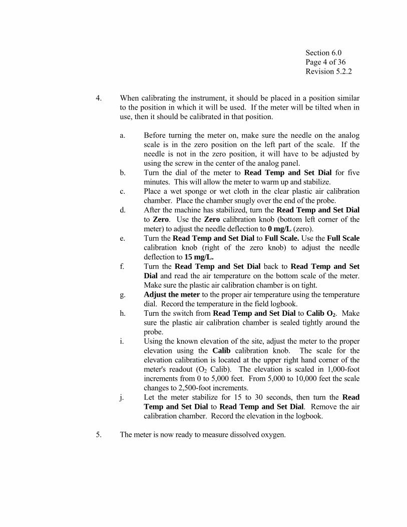
4. When calibrating the instrument, it should be placed in a position similar
to the position in which it will be used. If the meter will be tilted when in use, then it should be calibrated in that position.
a. Before turning the meter on, make sure the needle on the analog
scale is in the zero position on the left part of the scale. If the needle is not in the zero position, it will have to be adjusted by using the screw in the center of the analog panel.
b. Turn the dial of the meter to Read Temp and Set Dial for five minutes. This will allow the meter to warm up and stabilize.
c. Place a wet sponge or wet cloth in the clear plastic air calibration chamber. Place the chamber snugly over the end of the probe.
d. After the machine has stabilized, turn the Read Temp and Set Dial to Zero. Use the Zero calibration knob (bottom left corner of the meter) to adjust the needle deflection to 0 mg/L (zero).
e. Turn the Read Temp and Set Dial to Full Scale. Use the Full Scale calibration knob (right of the zero knob) to adjust the needle deflection to 15 mg/L.
f. Turn the Read Temp and Set Dial back to Read Temp and Set Dial and read the air temperature on the bottom scale of the meter. Make sure the plastic air calibration chamber is on tight.
g. Adjust the meter to the proper air temperature using the temperature dial. Record the temperature in the field logbook.
h. Turn the switch from Read Temp and Set Dial to Calib O2. Make sure the plastic air calibration chamber is sealed tightly around the probe.
i. Using the known elevation of the site, adjust the meter to the proper elevation using the Calib calibration knob. The scale for the elevation calibration is located at the upper right hand corner of the meter's readout (O2 Calib). The elevation is scaled in 1,000-foot increments from 0 to 5,000 feet. From 5,000 to 10,000 feet the scale changes to 2,500-foot increments.
j. Let the meter stabilize for 15 to 30 seconds, then turn the Read Temp and Set Dial to Read Temp and Set Dial. Remove the air calibration chamber. Record the elevation in the logbook.
5. The meter is now ready to measure dissolved oxygen.
Section 6.0 Page 5 of 36 Revision 5.2.2
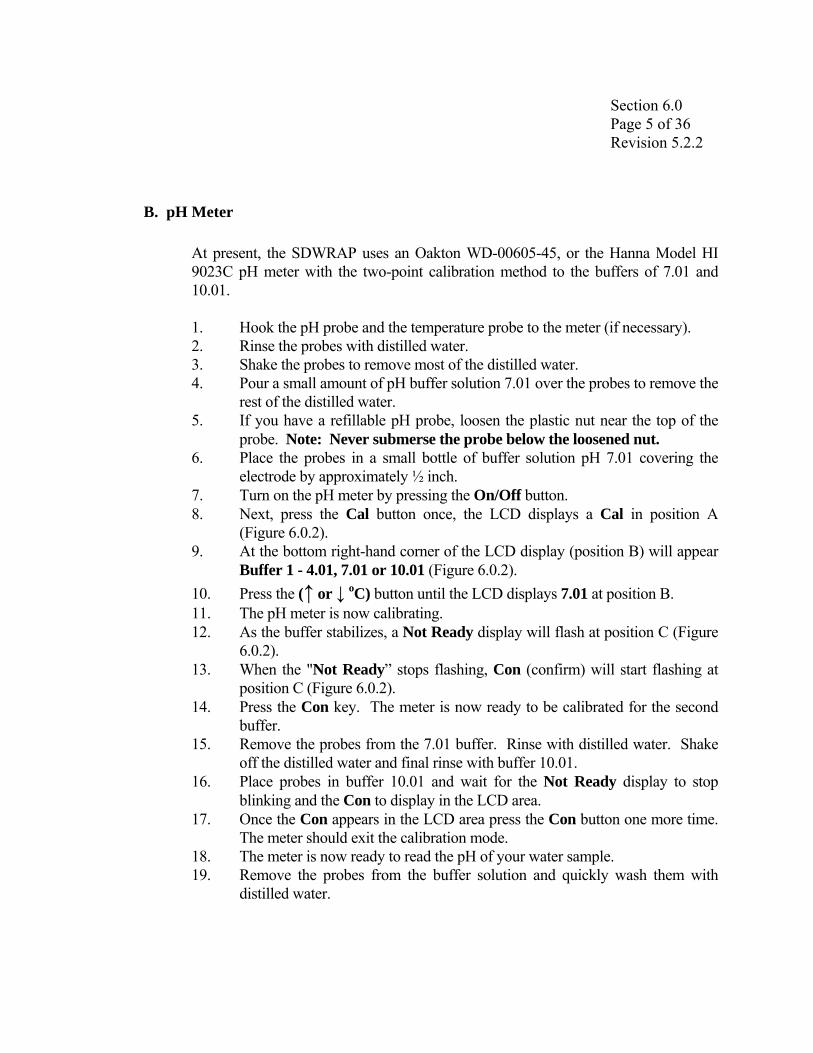
B. pH Meter
At present, the SDWRAP uses an Oakton WD-00605-45, or the Hanna Model HI 9023C pH meter with the two-point calibration method to the buffers of 7.01 and 10.01.
1. Hook the pH probe and the temperature probe to the meter (if necessary). 2. Rinse the probes with distilled water. 3. Shake the probes to remove most of the distilled water. 4. Pour a small amount of pH buffer solution 7.01 over the probes to remove the
rest of the distilled water. 5. If you have a refillable pH probe, loosen the plastic nut near the top of the
probe. Note: Never submerse the probe below the loosened nut. 6. Place the probes in a small bottle of buffer solution pH 7.01 covering the
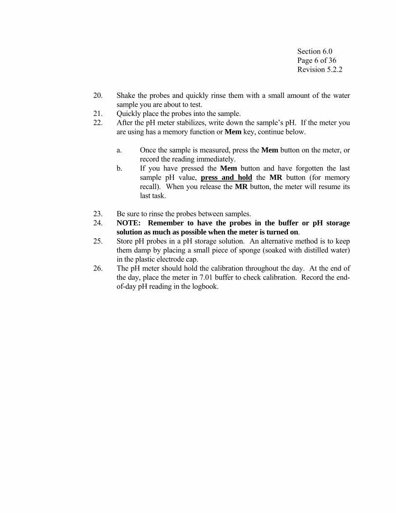
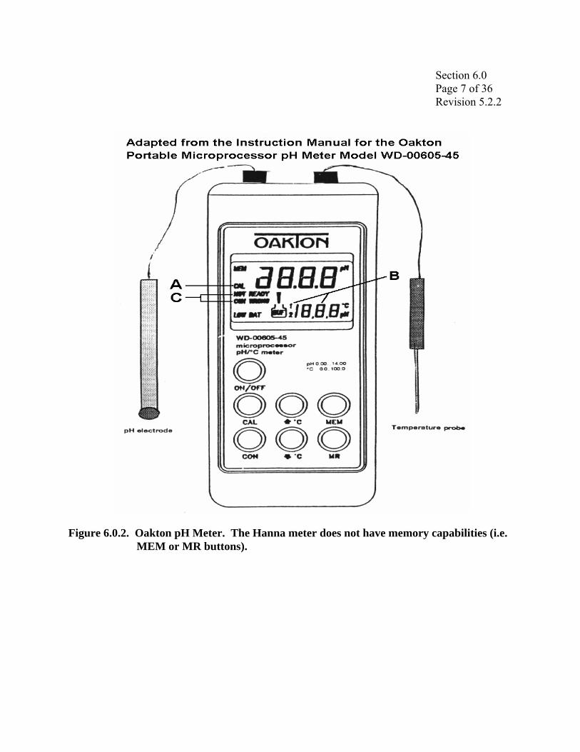
electrode by approximately ½ inch. 7. Turn on the pH meter by pressing the On/Off button. 8. Next, press the Cal button once, the LCD displays a Cal in position A
(Figure 6.0.2). 9. At the bottom right-hand corner of the LCD display (position B) will appear
Buffer 1 - 4.01, 7.01 or 10.01 (Figure 6.0.2). 10. Press the (↑ or ↓ oC) button until the LCD displays 7.01 at position B. 11. The pH meter is now calibrating. 12. As the buffer stabilizes, a Not Ready display will flash at position C (Figure
6.0.2). 13. When the "Not Ready” stops flashing, Con (confirm) will start flashing at
position C (Figure 6.0.2). 14. Press the Con key. The meter is now ready to be calibrated for the second
buffer. 15. Remove the probes from the 7.01 buffer. Rinse with distilled water. Shake
off the distilled water and final rinse with buffer 10.01. 16. Place probes in buffer 10.01 and wait for the Not Ready display to stop
blinking and the Con to display in the LCD area. 17. Once the Con appears in the LCD area press the Con button one more time.
The meter should exit the calibration mode. 18. The meter is now ready to read the pH of your water sample. 19. Remove the probes from the buffer solution and quickly wash them with
distilled water.
Section 6.0 Page 6 of 36 Revision 5.2.2
20. Shake the probes and quickly rinse them with a small amount of the water
sample you are about to test. 21. Quickly place the probes into the sample. 22. After the pH meter stabilizes, write down the sample’s pH. If the meter you
are using has a memory function or Mem key, continue below.
a. Once the sample is measured, press the Mem button on the meter, or record the reading immediately.
b. If you have pressed the Mem button and have forgotten the last sample pH value, press and hold the MR button (for memory recall). When you release the MR button, the meter will resume its last task.
23. Be sure to rinse the probes between samples. 24. NOTE: Remember to have the probes in the buffer or pH storage
solution as much as possible when the meter is turned on. 25. Store pH probes in a pH storage solution. An alternative method is to keep
them damp by placing a small piece of sponge (soaked with distilled water) in the plastic electrode cap.
26. The pH meter should hold the calibration throughout the day. At the end of the day, place the meter in 7.01 buffer to check calibration. Record the end-of-day pH reading in the logbook.
Section 6.0 Page 7 of 36 Revision 5.2.2
Figure 6.0.2. Oakton pH Meter. The Hanna meter does not have memory capabilities (i.e. MEM or MR buttons).

Section 6.0 Page 8 of 36 Revision 5.2.2
C. Conductivity Meter
1. Solution-Calibrated Conductivity Meter
a. Use a known standard solution. b. Rinse the probe with the known standard solution. c. Place the probe in the known solution. d. Adjust the reading on the dial to the proper conductivity
recommended by the manufacturer for that specific calibrating solution and for temperature at which the calibration has taken place.
2. Red Line-Calibration Method (YSI S-C-T Meter, Model 33).
a. Turn on meter. b. Turn meter to Calibration Mode. c. Let the meter warm up for approximately 5 minutes. d. Adjust the needle so it matches the red line on the analog display. e. The meter is now ready to take a reading. f. Select the proper scale, place the meter in the water and record the
conductivity. g. Periodically check the meter with a known solution. If the meter
does not calibrate properly or does not read close to the known conductivity solution, recondition the electrode according to manufacturer instructions.
D. Turbidity Meter
HF Scientific, Model DRT-15
a. Do not touch the bottom 2/3 of any glassware to be read by the turbidity meter (finger prints and smudges will affect reading accuracy). This section of the glass vial must be kept clean during use.
Section 6.0 Page 9 of 36 Revision 5.2.2
b. A calibration blank (glass vial containing de-ionized water) should be
kept with the turbidity meter. Hold this blank by the black cap and clean the glass with AccuWipe®, or any laboratory grade non-abrasive wipe, to remove spots, fingerprints, etc. Still holding the glass vial by the black cap, place the calibration blank into the optic well.
c. Turn the Range knob from the Off position to the 20 value, and let the meter warm up for 1 - 2 minutes.
d. Turn the REF ADJ dial until the display reads 0.02. e. The meter is now calibrated. Remove the calibration blank and place
the other glass vial containing the water sample, after it has been cleaned with AccuWipe®, into the optic well.
f. Record the reading.
E. Flow Meters
1. Marsh-McBirney Model 201 Flow Meter Calibrate the instruments in accordance with specific manufacturers instructions.
a. Turn the Range or Scale dial of the flow meter to Cal. b. The digital meter should read between “9.8” and “10.2” within 10
– 15 seconds. The analog meter needle should move to the darkened area marked Cal in the upper right-hand corner of the display.
c. If either meter does not calibrate properly, change batteries by removing the four screws in the back of the meter, replace the batteries and re-calibrate.
d. If the meter still does not calibrate correctly, call the project officer.
2. Aquacalc 5000
a. No calibration is needed for the Aquacalc flow meter.

Section 6.0 Page 10 of 36 Revision 5.2.2
F. CALIBRATION PROCEDURES for YSI Multi Meters
The following calibration procedures are for the most commonly used sensors. While calibrating the instrument, the operator must complete in detail the South Dakota YSI Calibration Worksheet for all applicable probes and sondes (Appendix A). For detailed information on all calibration procedures, refer to Section 2.9.2 of the Instruction Manual, Calibrate.
To ensure more accurate results, you can rinse the calibration cup with water, and then rinse the sensor that you are going to calibrate with a small amount of the calibration solution. Discard the rinse solution and add fresh calibrator solution. The correct amount of calibration solution will depend on the size of the sensor calibration cup.
1. Carefully immerse the probes into the solution and rotate the calibration
cup to engage several threads. YSI recommends supporting the sonde with a ring stand and clamp to prevent the sonde from falling over.
2. With a field cable connecting the sonde to the 650-MDS access the calibration menu.
3. The exact appearance of this menu will vary depending upon the sensors that are available and enabled on your sonde. To select any of the parameters from the Calibrate menu, highlight the parameter and press Enter. The following menu will vary depending on the parameter chosen, so refer to the following sections for details on calibrating each probe.
Note: Calibration of the Depth and Level sensor should be completed first at every site, followed by calibration of the Dissolved Oxygen sensor. The remaining sensors only need to be checked at the start of each sampling session.
4. After inputting the calibration value, or accepting the default value, press
Enter. A real-time display will appear on the screen. Carefully observe the stabilization of the readings of the parameter that is being calibrated. When the readings have been stable for approximately 30 seconds, press Enter to accept the calibration.
5. Press Enter to return to the Calibrate menu, and proceed to the next calibration.

Section 6.0 Page 11 of 36 Revision 5.2.2
6. If an Error message appears, begin the calibration procedure again. Be
certain that the value you enter for the calibration standard is correct. Also see Section 6 of the Instruction Manual, Troubleshooting for more information on error messages. If you continue to observe error messages during calibration, contact YSI Customer Service. See Section 8 of the Instruction Manual, Warranty and Service Information.
In the following sections, specific start-up calibration procedures are compiled for all sensors that commonly require calibration. If a sensor listed is not installed in your sonde, skip that section and proceed to the next sensor until the calibration protocol is complete. Before you use the sonde in the laboratory or field, read and study the detailed calibration information compiled in Section 2.9.2 of the Instruction Manual, Calibrate.
1. Temperature
Temperature does not require calibration, and is therefore not included in the Calibrate menu.
2. Depth and Level
For the Depth and Level calibration, you can leave the sonde set up the same way as for dissolved oxygen, in water-saturated air.
a. From the Calibrate menu, select number 3-Pressure-Abs (or
number 3-Pressure-Gage, if you have a vented level sensor) to access the depth calibration procedure. Input sensor offset in feet (difference between the pressure sensor and bottom of the sonde). Press Enter and monitor the stabilization of the depth readings with time. When no significant change occurs for approximately 30 seconds, press Enter to confirm the calibration. This zeroes the sensor with regard to current barometric pressure. Then press Enter again to return to the Calibrate menu.
b. For best performance of depth measurements, users should ensure that sonde orientation remains constant while taking readings. This is especially important for vented level measurements and for sondes with side-mounted pressure sensors.

Section 6.0 Page 12 of 36 Revision 5.2.2
3. Dissolved Oxygen (DO)
Probe Accuracy (DO Charge) DO charge (DOc) is an indicator of the condition of the dissolved oxygen probe and electrolyte solution. As the electrolyte in the sensor ages and depletes, the DOc will decrease from the optimal value of 50. As this happens, the DO readings will drift slightly lower. The minimum acceptable value for DOc is 25. When the DOc falls below 25 (less than 30) the electrolyte and membrane needs to be replaced. As the sensor tip ages and corrodes, the DOc will increase from the optimal value of 50. As this happens, the DO readings will drift slightly higher. The maximum acceptable value for DOc is 75. When the DOc climbs above 75 (greater than 85) the probe needs to be sanded and re-conditioned. If you do not know how to do this, please contact SD DENR. [For each probe there is a correlation between the DOc and the amount of drift seen in the DO values. However, there is no set correlation that may be used for all of the probes in general. Most of the probes tested resulted in less than 1mg/L shift in DO at the outer limits of the range (30-85), with some less than 0.1mg/L. After some use, re-conditioning and/or replacement of the electrolyte should not be expected to restore a DOc of 50]. DOc values between 40 and 60 should be expected and will produce accurate results. When DOc is out of range follow procedures below:
a. Obtain a YSI dissolved oxygen re-conditioning kit. b. Power down the YSI instrument (650 MDS). c. Carefully remove O-ring and DO membrane from the dissolved
oxygen probe. d. Rinse the DO probe with de-ionized water and carefully dry. e. Remove emery cloth (sandpaper) from the re-conditioning kit and
moisten with de-ionized water. f. Very lightly rub corroded/discolored DO electrodes with the emery
cloth until shiny (excessive sanding will damage the probe, so BE CAREFUL).
g. Rinse the probe with de-ionized water and carefully dry.
Section 6.0 Page 13 of 36 Revision 5.2.2
h. While holding the sonde inverted vertical, fill the probe sump and
electrodes with KCL solution (potassium chloride solution provided with the DO re-conditioning kit) until meniscus forms.
i. Remove new DO membrane from the re-conditioning kit. (Steps j through o are similar to Figure 6.0.1 (B through G, page 3)
j. Hold the probe in one hand and place the bottom edge of a membrane under the thumb of that same hand.
k. With your other hand, stretch the membrane up until it is about to break.
l. Then, quickly pull the membrane over the top of the probe and place the membrane under the index finger of the hand holding the probe.
m. Place the O-ring back over the membrane. n. Check for air bubbles. If air bubbles are present, repeat steps g
through m. o. Cut off any excess membrane, with scissors or knife. p. Power up the YSI instrument and observe the DOc value and
ensure that the DOc is in acceptable range. q. Continue with DO calibration procedure below. Place approximately 3 mm (1/8 inch) of water in the bottom of the calibration cup. Place the probe end of the sonde into the cup. Make certain that the DO and temperature probes are not immersed in the water. Engage only 1 or 2 threads of the calibration cup to ensure the DO probe is vented to the atmosphere. Wait approximately 10 minutes for the air in the calibration cup to become water saturated and for the temperature to equilibrate. Two calibration protocols are provided below for dissolved oxygen, one for sampling applications and one for long-term monitoring applications.

Section 6.0 Page 14 of 36 Revision 5.2.2
4. Sampling Applications
a. If the instrument will be used in sampling applications where the dissolved oxygen is pulsing continuously, Deactivate the “Autosleep” and “Wait for DO” as described in Section 2.6 of the Instruction Manual, Sonde Software Setup. Under these conditions the user retains manual control of the calibration routines, viewing the stabilization of the readings in real time and confirming the calibration with keystrokes.
i. From the Calibrate menu, select number 2-Dissolved Oxy,
then number 1-DO % to access the DO percent calibration procedure. Calibration of dissolved oxygen in the DO % procedure also results in calibration of the DO mg/L mode, and vice versa.
ii. Enter the current barometric pressure in mm of mercury (Hg). (Inches of Hg x 25.4 = mm Hg).
iii. Note: Barometer readings that appear in meteorological reports are generally corrected to sea level and are not useful for calibration procedures unless they are uncorrected.
iv. To un-correct barometric pressure readings follow procedures below.
aa. Determine local altitude from topographic map or
altimeter. bb. Obtain barometric pressure reading (BP) from
nearest location (airport or town). cc. Calculate the correction factor (CF):
CF = 760 – (Altitude x 0.026) 760
dd. The un-corrected barometric pressure = Corrected
BP x CF. ee. Convert un-corrected reading to mm/Hg (follow
step ii).

Section 6.0 Page 15 of 36 Revision 5.2.2
v. Press Enter and the current values of all enabled sensors
will appear on the screen and change with time as they stabilize. Observe the readings under DO %. When they show no significant change for approximately 30 seconds, press Enter. The screen will indicate that the calibration has been accepted (successful) and prompt you to press Enter again to return to the Calibrate menu.
vi. Rinse the probes and calibration cup in de-ionized water and carefully dry probes and cup to begin conductivity calibration.
b. If the instrument will be used in longer-term monitoring where
power is only applied to the sensors during sampling or calibration, Activate - Autosleep RS232 and Wait for DO as described in Section 4.6 of the Instruction Manual, Advanced. In this mode the 650 MDS will go to sleep after 1 minute of inactivity. The sonde will warm up the sensors for the period of time selected for the DO sensor (DO warm up time; see section 4.6 of the instruction manual). Under these conditions the user will lose manual control of the calibration routine; each parameter will automatically calibrate after the time selected for warm up of the DO sensor has expired. In this mode of calibration, the user will not observe the readings in real time, but instead will observe a countdown of the warm-up period followed by a message indicating that the calibration is complete.
5. Conductivity This procedure calibrates conductivity, specific conductance, salinity, and total dissolved solids.
a. Place the correct amount of conductivity standard into a clean, dry
or pre-rinsed calibration cup. b. For maximum accuracy, the conductivity standard you choose
should be within the same conductivity range as the water you are preparing to sample. However, we do not recommend using standards less than 1 mS/cm. For example:
Section 6.0 Page 16 of 36 Revision 5.2.2
" For fresh water, use a 1 mS/cm conductivity standard. " For brackish water use a 10 mS/cm conductivity standard. " For seawater use a 50 mS/cm conductivity standard.
The SD WRAP uses 1,413 µS/cm (1.413 mS/cm) @ 25 °C conductivity standard
c. Before proceeding, ensure that the sensor is as dry as possible.
Ideally, rinse the conductivity sensor with a small amount of standard solution that can be discarded. Be certain that you avoid cross-contamination of standard solutions with other solutions. Make certain that there are no salt deposits around the oxygen and pH probes, particularly if you are employing standards of low conductivity.
d. Carefully immerse the probe end of the sonde into the solution. Gently rotate and/or move the sonde up and down to remove any bubbles from the conductivity cell. The probe must be completely immersed in calibration solution past its vent hole. Use a volume that ensures that the vent hole (the 1 cm opening in the conductivity probe) is covered.
e. Allow at least one minute for temperature equilibration before proceeding.
f. From the Calibrate menu, select number 1-Conductivity to access the Conductivity calibration procedure and then number 1-SpCond to access the specific conductance calibration procedure. Enter the calibration value of the standard you are using (µS/cm at 25°C) and press Enter. The current values of all enabled sensors will appear on the screen and will change with time as they stabilize.
g. Observe the readings under Specific Conductance or Conductivity. When they show no significant change for approximately 30 seconds, press Enter. The screen will indicate that the calibration has been accepted (successful) and prompt you to press Enter again to return to the Calibrate menu.
h. Rinse the probe and calibration cup in de-ionized water and carefully dry afterward to begin pH calibration.

Section 6.0 Page 17 of 36 Revision 5.2.2
6. pH 2-Point
Using the correct amount of pH 7.01 buffer standard in a clean, dry or pre-rinsed calibration cup, carefully immerse the probe end of the sonde into the solution. Allow at least 1 minute for temperature equilibration before proceeding.
a. From the Calibrate menu, select number 4-ISE1 pH to access the
pH calibration choices and then press number 2-2-Point. Press Enter and input the value of the buffer (7.01 in this case) at the prompt. Press Enter and the current values of all enabled sensors will appear on the screen and change with time as they stabilize in the solution. Observe the readings under pH and, when they show no significant change for approximately 30 seconds, press Enter. The display will indicate that the calibration is accepted.
b. After the pH 7 calibration is complete, press Enter again, as instructed on the screen, to continue. Rinse the sonde in water and dry the sonde before proceeding to the next step.
c. Using the correct amount of an additional pH buffer standard (usually pH 10.01) into a clean, dry or pre-rinsed calibration cup, carefully immerse the probe end of the sonde into the solution. Allow at least 1 minute for temperature equilibration before proceeding.
d. Press Enter and input the value of the second buffer at the prompt. Press Enter and the current values of all enabled sensors will appear on the screen and will change with time as they stabilize in the solution. Observe the readings under pH and, when they show no significant change for approximately 30 seconds, press Enter. After the second calibration point is complete, press Enter again, as instructed on the screen, to return to the Calibrate menu.
e. Rinse the sonde in water and dry. Thoroughly rinse and dry the calibration containers for future use.
The next calibration instructions are only for the 6820, 6600 and 6920 sondes. If you do not have one of these sondes, disregard remaining calibration procedures.

Section 6.0 Page 18 of 36 Revision 5.2.2
7. Turbidity 2-Point
Select 8-Turbidity from the Calibrate Menu and then 2-2-Point. NOTE: One standard must be 0 NTU, and this standard must be calibrated first.
a. To begin the calibration, the correct amount of 0 NTU standard
(clear, de-ionized, distilled, or tap water) into the clear calibration cup (provided) or in a glass beaker. Input the value 0.00 NTU at the prompt, and press Enter. The screen will display real-time readings that will allow you to determine when the readings have stabilized. If you have a mechanically cleaned turbidity probe installed, activate the wiper 1-2 times by pressing number 3-Clean Optics as shown on the screen to remove any bubbles. If your probe is not mechanically cleaned, rotate the sonde back and forth in the water to facilitate removal of bubbles. After stabilization is complete, press Enter to “confirm” the first calibration and then, as instructed, press Enter to continue.
b. Dry the sonde carefully and then place in the second turbidity standard (10 NTU is suggested) using the same container as for the 0 NTU standard. Input the correct turbidity value in NTU, press Enter, and view the stabilization of the values on the screen in real-time. As above, activate the wiper with the “3” key or manually rotate the sonde to remove bubbles. After the readings have stabilized, press Enter to “confirm” the calibration and then press Enter to return to the Calibrate menu.
c. Thoroughly rinse and dry the calibration cups for future use.
8. Chlorophyll a 1-Point
Select Optic Chlorophyll from the Calibrate Menu and then select Chl µg/L. Then select 1-1 Point. NOTE: This procedure will zero your fluorescence sensor and use the default sensitivity for calculation of chlorophyll concentration in µg/L. The default sensitivity is usually within 25 % for any probe. The 1-point calibration will therefore allow quick and easy fluorescence measurements that are only semi-quantitative with regard to chlorophyll. However, the readings will reflect changes in chlorophyll from site to site, or over time at a single site.

Section 6.0 Page 19 of 36 Revision 5.2.2
To increase the accuracy of your chlorophyll measurements, follow the 2-point or 3-point calibration protocols outlined in Section 2.9 of the Instruction Manual, Sonde Menu. Before making any field readings, carefully read Sections 5.12, Chlorophyll and Appendix I of the Instruction Manual, Chlorophyll about chlorophyll that describes practical aspects of fluorescence measurements.
a. To begin the calibration, place the correct amount of clear de-
ionized or distilled water into the YSI clear calibration cup provided or in a glass beaker of an appropriate size (600 mL for 6820 and 6920 sondes; 800 mL for the 6600 sonde). With the probe guard installed, immerse the sonde in the water. Input the value 0 µg/L at the prompt, and press Enter. The screen will display real-time readings that will allow you to determine when the readings have stabilized. Activate the wiper 1-2 times by pressing number 3-Clean Optics as shown on the screen to remove any bubbles from the sensor. After stabilization is complete, press Enter to “confirm” the calibration and then, as instructed, press Enter to return to the Calibrate menu.
b. Thoroughly rinse and dry the calibration cups for future use. For additional information related to calibrating the chlorophyll sensor, refer to Sections 5.12 of the Manufacturers Instruction Manual, Chlorophyll and Appendix I of the Instruction Manual, Chlorophyll.
9. YSI Calibration Reset Procedure
The reset procedure should be used if errors are encountered during calibration (indicates that the meter is set out of the solution range).
a. Turn the YSI 650 MDS to On. b. Select the Sonde menu. c. From this menu select the Advanced. d. Next select the Cal constants (first menu selection). e. After selecting, make sure all of the values on the YSI are the same
as those found in Table 6.0.1. If they are not within the operating range listed in Table 6.0.1, make note of those incorrectly set and press the Escape key two times to return to the main menu.
f. Select Calibrate from the menu.

Section 6.0 Page 20 of 36 Revision 5.2.2
g. Select the one of the parameters that were out of adjustment and
enter through options until required to enter the calibration value. h. Hold down the Enter key and press Esc. At the “Uncal?” prompt
select Yes and press Enter. i. Repeat steps g-h for each of the values that are out of adjustment.
Table 6.0.1. YSI calibration constants

Section 6.0 Page 21 of 36 Revision 5.2.2
10. YSI Data Download Procedure
a. Install download cable to 650 MDS and connect to the serial port
(Com 1) on the computer. b. Turn on computer and open EcoWatch software. c. Select Comm, settings and Port Setup. d. Select Com Port (Com 1) used by computer under Settings for
Port. e. For “Port Parameters” select Baud - 9600, Data – 8-bits and Parity
– None. f. For “Protocol” select Kermit. g. For “Handshaking” select XonXoff. h. Select OK to accept these settings. i. Select Comm, Terminal and Com 1; a dialog box will appear and
the program is ready to accept data. j. Power up 650 MDS. k. Select Communications, Enter. l. Select Kermit 650 PC, Enter. m. Select desired file(s) to transfer or All Files, Enter. n. Each transferred file is transferred as a *.dat file in the EcoWatch
program under ECOWIN/Data. 11. Creating Site List on YSI 650 MDS
a. Turn on YSI 650 MDS. b. Select “Logging Setup”. c. Check :Use Site List” (display options will increase). d. Select “Edit Site List”. e. Enter sites as needed.
G. Stage Recorders and Data Loggers
A variety of stage recorders and data loggers are used by WRAP, each with different setup, download and calibrating methods. Specific device methods are given in the following sections. Calibrate each instrument in accordance with the manufacturer instructions. If problems occur, contact the project officer or the manufacturer.

Section 6.0 Page 22 of 36 Revision 5.2.2
ISCO GLS Auto Samplers used in Combination with 4230 Flow Meters
The following list should be used when programming the ISCO 4230 Flow Meter when it is used in combination with the ISCO GLS auto sampler.
1. ISCO 4230 Flow Meter
a. After connecting the power cable to the 4230 unit, Turn it On. b. Press the Enter Program button. c. Select Program and press Enter button. d. Measure Level Units in Feet and press Enter button. e. Flow Rate units of measure – Not Measured. f. pH units of measure – Not Measured. g. DO units of measure – Not Measured. h. Temp units of measure – Not Measured. i. YSI 600 connected – No. j. Parameter to Adjust – Level. k. Set to 0 with the bubble line connected but not submerged l. Parameter to Adjust – None. m. Sampler Pacing – Disabled. n. Sampler Enable Mode – Conditional. o. Condition – Level. p. Level greater than – Enter. q. Level greater than – (Water Depth + 0.2 ft). r. Operator Done. s. When enable conditions no longer met – Keep Enabled. t. IF enable currently latched, Reset? – Yes. u. Plotter on/off with enable – Yes. v. Plotter Speed – Off. w. Report Generator A – Off. x. Report Generator B – Off. y. Print History – No. z. Clear History – No.
The final screen should display the Depth and Date on the first line and the time followed by a letter D on the second line. If there is a letter E on the second line that persists for more than a minute, attempt to reprogram the unit, paying careful attention to steps o through r.

Section 6.0 Page 23 of 36 Revision 5.2.2
Programming the GLS unit should be done following the programming of the 4230.
2. ISCO GLS Sampler
a. After connecting the GLS unit to the 4230, turn it On. b. Select the Program Menu and press Enter button. c. Select Time-paced sampling. d. Set the pacing interval for 15 minutes. e. Set the bottle size to 9600 ml. f. Select 6 samples to be collected. g. Set the volume to be collected to 1000 ml. h. Set the time to first sample to 1 minute. i. After completing the program a timer will count down for 1 minute
at which point the sampler will display the message Sampler Inhibited.
j. If the sampler begins to take a sample, power the unit down and recheck the programming for the 4230 to ensure that no mistakes were made.
Section 6.0 Page 24 of 36 Revision 5.2.2
3. ISCO 6700 Auto Sampler with 730
NOTE: After completing each step, pressing the ENTER key moves to the next step.
a. After connecting the power cable to the 6700 unit, Turn it On. b. Make sure that Program is highlighted on the screen. c. Name the site according to the PIP. d. Measure Level Units in Ft (feet). e. Units selected should be set to Ft. f. The flow rate should be set to CFS and the flow should be set to
CF. g. The bubble module should be set to Level Only. h. With the bubble line connected, but not submerged, set the level to
0. i. Set the Data interval to 15 minutes. j. Set the suction line length to the length of tubing to be used at that
station. k. Make sure that the unit is set to Auto Suction Head. l. Make sure that the unit is set for 1 rinse and 1 retry. m. Select 1 part program. n. Set the pacing time interval to 15 minutes. o. Set for a composite of 4 samples. p. Set the volume to be collected at 1100 ml. q. Set the enable depth to 0.2 foot greater than the actual depth. r. Set the enable feature to read Once enable, stay enable. s. Set the unit for 0 purges and resumes. t. Make sure that the No delay to Start option is selected. u. When the unit requests if you would like to run the program, select
Yes.
4. Downloading ISCO 4230 and 6700 Samplers (Rapid Transfer Device)
a. Equipment used is a model 581 Rapid Transfer Device (RTD). b. Insert the male end of the RTD into the interrogator connection
port on the ISCO4230 and the 6700 sampling devices.

Section 6.0 Page 25 of 36 Revision 5.2.2
c. When connected the power light (middle amber light) will
illuminate and data will also begin to be transferred (indicated by a flashing green light).
d. When download is complete, the green indicator light will remain on.
e. If while transferring data, a problem is encountered the red light will flash.
f. If while downloading the RTD unit, the red light comes on, this indicates the memory is full.
g. Detach the RTD unit from the sampler and return to the office to download sampler data to the computer. Note many data files are able to be downloaded on the RTD device.
4.1. Downloading Rapid Transfer Device (RTD) to Computer (Flowlink
4.12 Software) a. Equipment needed for downloading the RTD device is an ISCO
RTD Power Cable. b. Attach the serial connector to the serial port on the computer (Com
1), plug the female connector into the RTD and plug the power cord into a wall outlet (the amber power light will flash).
c. Open Flowlink 4.1 software on the computer. d. A Connect interface dialog box will come up on the screen. e. Click Cancel to access the Flowlink 4.1 program. f. Either select “File:, “RTD Transfer” or click the RTD symbol
button. g. The RTD will immediately begin to download to the software. h. When the transfer is complete, the download dialog box will
disappear. i. Data is ready to be analyzed.
5. OTT Thalimedes
Configuring the OTT Thalimedes (Hydras 3 software). This procedure initializes the OTT Thalimedes and sets the unit for stage recording data collection.
Section 6.0 Page 26 of 36 Revision 5.2.2
5.1. Initial Setup
a. Start the Hydras 3 software and select New Workspace under the
File menu. b. Use the name of your project to name the workspace. c. Double click Hydras 3 to create path d. Once the workspace is created, click the (+) sign next to the
Workspace. e. Highlight All Stations. f. Select Communication and Read / Operate from the Hydras 3
menu. g. Select Thalimedes from the sensor type menu. Make sure the
Protocol type is set at OTT Protocol 2 (selective) and select IrDA LinkIt Adapter, COM1, 19200Bd, 8N1 under Communication path.
h. Select Configuration Hydrosens (Matrix) or Orphim/Thalim/Nimbus.
i. Connect the IrDA LinkIt Adapter to a serial cable and attach it to the serial port (COM1) on the computer.
j. Wake the Thalimedes by placing your hand over the infrared motion sensor (two red sensors at the lower left corner of the display) until the display is visible (approximately 2-4 seconds).
k. While pointing the reader at the IrDA interface sensor on the Thalimedes, select Start.
l. After the computer uploads the sensor data, make sure that:
(i) Input new Station Name and Number. (ii) Select Units in feet or meters. (iii) Set the sensor to sample every 5 minutes (Sample
interval) and record every 15 minutes (Storage interval). (iv) Measure the Stage and check box next to Meas. Value – set
new and enter new stage. (v) During initial setup check Erase Data Storage Box. (vi) Check Set date / time (PC time) Box. (vii) Select Set Clock to PC time (viii) Make sure that the Baud rate RS232C is set at 19,200.
m. Wake the Thalimedes unit and place IrDA LinkIt Adapter over the
IrDA interface sensor on the Thalimedes.

Section 6.0 Page 27 of 36 Revision 5.2.2
n. Select Program. o. Select Exit. p. Select Standard (selective) under Read data. q. Make sure the All sensors and the All box under dates are
checked. r. Select Start (information will show up in the bottom left corner of
the Hydras 3 Communication screen). s. When complete, click End. t. Select Communication and Raw data management from the
Hydras 3 menu. The unit (file) that was just downloaded is highlighted.
u. Click the Selected button that will transfer the data to the station and sensor.
v. A Confirm screen will come up stating that the station (for this workspace) has not been entered! Create new entry? Select Yes.
w. Another confirm screen will come up stating that the sensor (for this station) has not been entered! Create new entry? Select Yes.
x. Close Raw data management window. y. Once window closes, click the (+) sign next to the All Station and
make sure the new station shows up on the ‘all station’ list. z. Click the (+) sign next to the New Station and make sure the
sensor is listed. aa. Double click on the sensor to bring up the Evaluation screen. bb. The unit is now programmed and ready for use at that site. 5.2. Downloading Data (OTT Thalimedes)###
a. Start the Hydras 3 software. b. Select (highlight) the desired project (workspace). c. Connect the IrDA LinkIt Adapter to a serial cable and attach it to
the serial port (COM1) on the computer. d. Click the (+) sign next to the highlighted project. e. Click the (+) sign next to the All Stations. f. Highlight specific station for downloading. g. Select Communication and Read / Operate from the Hydras 3
menu. h. Select Thalimedes from the sensor type menu. Make sure the
Protocol type is set at OTT Protocol 2 (selective) and select IrDA LinkIt Adapter, COM1, 19200Bd, 8N1 under Communication path.
Section 6.0 Page 28 of 36 Revision 5.2.2
### If unable to connect or download data with the IrDA LinkIt Adapter, follow the instructions below to direct connect the OTT Thalimedes.
f. Obtain one short (female-female) RS-232 serial cable (non-
modem cable). g. Cut the serial cable approximately 9 inches from each end to
create two useable connection/download cables (one cable for each OTT Thalimedes unit that has difficulty connecting/downloading).
h. Unscrew the battery cap and remove the battery and cap. i. Grasp the clear cover over the Thalimedes unit and press firmly
down to remove the cover exposing the circuit board. j. Remove the protective cap next to the permanently wired cap at
the end of the unit. k. Break out the end of the cap and thread the cut end of the serial
cable created in step “b” through the non-threaded end of cap until one inch of the cable is through the cap.
l. Strip off ¾ of an inch of the outside protective cover to reveal the wires inside.
m. Separate the Red, Brown and Yellow wires. n. Cut the remaining wires off flush with the end of the protective
cover (¾ of an inch) serial cable. o. Strip off 3/8 of an inch of the outside protective cover of each Red,
Brown and Yellow wire. p. Using a small flat tip screwdriver, attach wires to bus connector
locations described below:
Wire Color Bus Location Red RXD Brown TXD Yellow GND
q. Grasp the clear cover over the Thalimedes unit and press firmly
upward to replace the protective cover over the circuit board. r. Replace the battery and screw on the battery cap. s. The unit is now ready to directly download.
Section 6.0 Page 29 of 36 Revision 5.2.2
i. Check the box in front of Standard (selective). j. Make sure the All sensors and All box under dates are checked. k. Wake the Thalimedes unit and place IrDA LinkIt Adapter over the
IrDA interface sensor on the Thalimedes. l. Select Start (information will show up in the bottom left corner of
the Hydras 3 Communication screen). m. When complete, click End. n. Select Communication and Raw data management from the
Hydras 3 menu. The unit (file) that was just downloaded is highlighted.
o. Click the Selected button transfer the data to the station and sensor.
p. Click the (+) sign next to the station just transferred. q. Double click on the sensor to bring up the Evaluation screen to
view and analyze data. r. Repeat above procedure at all remaining stations.
6. Configuring the OTT Nimbus (Hydras 3 software). This procedure initializes the OTT Nimbus and sets the unit for stage recording data collection. 6.1. Initial Setup
a. Start the Hydras 3 software. b. If adding a station/sensor to existing project, start at step “h.” c. If creating new Workspace (Project) start at step “d.” d. Select New Workspace under the File menu. e. Use the name of your project to name the workspace. f. Double click Hydras 3 to create path. g. Once the workspace is created, click the (+) sign next to the
Workspace. h. Highlight All Stations. i. Select Communication and Read / Operate from the Hydras 3
menu. j. Select Nimbus from the sensor type menu. Make sure the
Protocol type is set at OTT Protocol 2 (selective) and select RS232C/ V.24, COM1, 19200Bd, 8N1 under Communication path.
Section 6.0 Page 30 of 36 Revision 5.2.2
k. Select Configuration Hydrosens (Matrix) or
Orphim/Thalim/Nimbus. l. Attach 12-volt battery to power up the Nimbus unit.
Note: When initial power is applied to the Nimbus unit the pump will run for 6 minutes before a reading (measured value) is available.
m. Connect the serial cable (Cable ends need to be: female/female)
and attach it to the serial port (COM1) on the computer. n. Attach the other end of the serial cable to the serial connector on
the Nimbus unit. o. Click Start. p. After the computer uploads the sensor data, make sure that:
i. Input new Station Name and Number (unique). ii. Select Units in feet or meters. iii. Set the sensor to sample every 5 minutes (Sample interval)
and record every 15 minutes (Storage interval). Note: After connecting to the Nimbus unit the pump runs for 40 seconds before a reading (measured value) is available.
iv. Measure the stage and check box next to Meas. Value –
set newly and enter new stage. v. During initial setup check Erase Data Storage Box. vi. Check Set date / time (PC time) Box. vii. Select Set Clock to PC time viii. Make sure that the Baud rate RS232C is set at 19,200.
q. Select Program. r. Select Exit. s. Select Standard (selective) under Read data. t. Make sure the All sensors and All box under dates are checked. u. Select Start (information will show up in the bottom left corner of
the Hydras 3 Communication screen). v. When complete, click End.

Section 6.0 Page 31 of 36 Revision 5.2.2
w. Select Communication and Raw data management from the
Hydras 3 menu. The unit (file) that was just downloaded is highlighted.
x. Click the Selected button transfer the data to the station and sensor.
y. A confirm screen will come up stating that the station (for this workspace) has not been entered! Create new entry? Select Yes.
z. Another confirm screen will come up stating that the sensor (for this station) has not been entered! Create new entry? Select Yes.
aa. Close Raw data management window. bb. Once window closes, click the (+) sign next to the All Station and
make sure the new station shows up on the all station list. cc. Click the (+) sign next to the New Station and make sure the
sensor is listed. dd. Double click on the sensor to bring up the Evaluation screen. ee. The Unit is now programmed and ready for use at that site. 6.2. Downloading Data (OTT Nimbus)
a. Start the Hydras 3 software. b. Connect the serial cable (Cable ends need to be: female/female)
and attach it to the serial port (COM1) on the computer. c. Attach the other end of the serial cable to the serial connector on
the Nimbus unit. d. Select (highlight) the desired project (workspace). e. Click the (+) sign next to the highlighted project. f. Click the (+) sign next to the All Stations. g. Highlight specific station for downloading. h. Select Communication and Read / Operate from the Hydras 3
menu. i. Select Nimbus from the sensor type menu. Make sure the
Protocol type is set at OTT Protocol 2 (selective) and select RS232C/ V.24, COM1, 19200Bd, 8N1 under Communication path.
j. Check the box in front of Standard (selective). k. Make sure the All sensors and the All box under dates are
checked. l. Select Start (information will show up in the bottom left corner of
the Hydras 3 Communication screen).

Section 6.0 Page 32 of 36 Revision 5.2.2
m. When complete, click End. n. Select Communication and Raw data management from the
Hydras 3 menu. The unit (file) that was just downloaded is highlighted.
o. Click the Selected button transfer the data to the station and sensor.
p. Click the (+) sign next to the station just transferred. q. Double click on the sensor to bring up the Evaluation screen to
view and analyze data. r. Repeat above procedure at all remaining stations.
7. Stevens Type F Stage Recorders
Maintenance of Stevens recorders should be completed weekly during periods of discharge. During periods when a site has no water flow, the clock may be adjusted (Step ii of ”paper installation”) to 16 allowing inspection and maintenance to be carried on once every two weeks.
a. Paper Removal
i. Rotate the marking pen so that it no longer contacts the
current sheet. ii. Adjust the spring bands so that the graph paper may be
removed without tearing. iii. Circle the point on the graph paper where the marking pen
was last located and write the current date and time on the graph paper next to the circle.
b. Paper Installation
i. Write the date, time, and site number along the edge of a
clean sheet of graph paper. ii. Make sure that the timer dial is set to 8 on the clock. iii. Place the new sheet of graph paper on the cylinder making
sure that the notch in the paper aligns with the peg on the cylinder and that all lines on the graph align with each other.
iv. Place the spring retaining clips on each end of the paper.

Section 6.0 Page 33 of 36 Revision 5.2.2
v. Adjust the marking pen so that when facing the clock, it is
located on the left side of the cylinder to the right of the spring retainer.
vi. Manually rotate the pulley a couple of inches each direction and visually note that the marking pen is making contact.
8. R2 Data Logger Setup, Calibration, and Downloading Method The R2 data logger is a stage recorder which using a float and pulley system and records the change in stage electronically. A laptop computer is required with an RS232 cable (Cable ends need to be male : female) in order to program the logger and download information from it.
a. Setup (Installing the stilling well and the gauging house)
i. Insure that the gauging house is level so that the cable for
the float/weight and pulley system is unobstructed and is allowed to freely move up and down inside of the stilling well. Measure the depth of water inside the stilling well.
ii. The R2 unit with the pulley and potentiometer is placed in the gauging house. The cable length for the weight and pulley should be long enough so that if the stream dries out the float will not go completely up and over the pulley. In addition, there should be enough length in the cable to allow the float to completely go to the top of the pulley if the water depth in the stream should get that high.
iii. Place the beaded cable into the slot on the pulley making sure that the beads slide into holes in the pulley. Adjust the cable according to depth of water in the stilling well so that the entire length of the cable can be used if the water depth should increase or decrease substantially.
iv. Insert a fully charged 12-volt battery into the R2 unit. v. After the float and weight have been placed on the pulley
and the battery installed, the R2 needs to be hooked up to the laptop computer so that it can be calibrated and programmed.
Section 6.0 Page 34 of 36 Revision 5.2.2
vi. Hook up the RS232 cable to the R2 unit inside the square
gray box. Inside of this container there should be a serial port for the RS232 cable. The cable then needs to be attached to a COM port in the back of the laptop computer (9 pin).
vii. After attaching the computer to the R2 unit via the RS232 cable, turn the computer on and go into Windows Explorer. You will need to have the R2PC software that came with the R2 unit. Go into Windows Explorer and the R2PC subdirectory. Double click on the R2PC2000.exe file to open the program. You may have to do this several times before the program actually opens up. If the message displayed reads “Runtime error 200 at 0CAF:0091,” close the window and double click on the R2PC2000.exe file again. If the software does not open, call the Project Officer to request a updated copy of R2PC2000.
viii. The program is ready when the R2PC window says “Specify com port (1-4) for R2 Logger Communications:” Specify which COM port that the RS232 cable has been plugged into in the back of the computer, which is usually 1. Select Enter.
ix. At the next screen there will be three menus on top of the open window. With the mouse, point and click on Logger at Com #. This will present a dropdown list for 9600 or 1200 baud rate. Select 9600 baud.
x. If the computer is plugged into the R2 logger then the action described in step ix should wake up the logger. A series of commands (menu) will come up. This will depend upon whether the battery is fully charged or all the connections are working correctly. If the commands do not come up, then something is wrong. The cable, the connectors, or the battery should be changed or adjusted.
xi. If the command screen does come up, Enter command: Status. ‘Status’ will bring up information pertaining to the site name, whether or not it is currently logging, amount of remaining memory, status of the batteries, etc.

Section 6.0 Page 35 of 36 Revision 5.2.2
b. Calibration
To insure that the proper depth is going to be recorded, the logger must be adjusted to the water depth (stilling well) collected in step ‘i’ of the setup section. To calibrate the logger, the float and weight must be properly adjusted as described in steps ‘i’ through ‘iv’ in the setup section.
i. Enter Command: Scan. Then enter the time between scans,
i.e. one or two seconds where “Scan Repeat Interval” is displayed. Select Enter. A continuous depth reading should appear on the computer screen.
ii. Make sure the float and weight are on the correct side by moving the pulley back and forth while monitoring the computer screen. When the float moves up in the stilling well the computer should indicate an increase in depth. If the depth decreases then the float and weight must be switched around on the pulley so that the upward movement of the float indicates an increase in depth.
iii. Once the weight and float have been put on the pulley in the correct direction with the proper length, the R2 logger can be calibrated.
iv. On the end of the pulley there should be a nut or wingnut. Loosen the nut or wingnut but do not take it completely off.
v. While monitoring the screen and keeping the pulley stationary, carefully rotate the shaft going between the pulley and the potentiometer. Rotate the shaft until the correct depth on the computer screen appears.
vi. Once the shaft has been adjusted so that the proper depth is being recorded, re-tighten the wingnut on the shaft to keep the float and pulley on the correct depth reading.
vii. Recheck the depth measurement on the screen once the nut is tight and hands are free of the wheel and the unit. Readjust as needed.
c. Logging Program
i. After the wingnut has been retightened, select Escape on
the computer to stop the scanning procedure.

Section 6.0 Page 36 of 36 Revision 5.2.2
ii. Select Control–M to bring up the menu options again. iii. Enter Command: Status. Select Enter. iv. The computer should show how much memory is currently
available. However, before programming in the current site information, the memory should be purged.
v. Enter Command: Purge. {Deleting old records. How many of the most recent records should be retained? 1 to 900}. All records should be deleted. This will completely purge the entire memory. The Start command allows you to completely clear the data memory.
vi. Purge is not needed if using circular memory. vii. If the time was incorrect for the monitor, Enter Command:
Time. Change the time (if necessary) listed on the R2 unit. Select Enter. Note: time is in 24-hour time.
viii. Enter Command: Start. This will start the programming operation for the R2 logger. Select Enter.
ix. Type in the Station ID. x. Type in the Recording Interval: Example: Record every
15 minutes or 900 seconds. Note that recording more often will use memory capacity faster and the time between downloading information will need to be shorter (e.g. 30 days vs. 15 days).
xi. New Scan Interval (secs): Scan approximately every 5 minutes or 300 seconds or whatever the scan interval has been decided upon to determine the average for the recording interval described in step ‘x’, above.
xii. Type in a Start Time. Default is Now. xiii. Log file already exists. Erase or Append? (E,A, ESC): In
most instances you will want to erase an old log file. However, if you are downloading information on a more regular basis and there is enough memory you may want to append the existing log file.
xiv. Circular Memory (Y, N): Note that choosing ‘N’ will result in the termination of logging operations once the memory capacity has been reached. Enabling circular memory means that when the data memory is exhausted, the logger will write over the oldest data instead of halting logging.

Section 6.0 Page 37 of 36 Revision 5.2.2
xv. At this point, if the default start (now) was chosen, then the
“Logging is Active. Start current date and current time” message should appear on the screen.
xvi. Type in Status at the cursor. At some point on the screen should be an estimate as to how much time is available for logging based on the scanning and recording interval. The logger will need to be downloaded before this time expires.
xvii. Type in Bye or unplug the R2 from the computer. The R2 will automatically go to sleep within 5 minutes if there is no activity to keep it awake.
xviii. The R2 logger can than be left until downloading occurs. Close the unit case and shut the gauging house.
d. Downloading
i. Go through steps ‘iv’ through ‘ix’ in the setup section. ii. After the logger is awake and the command screen is up
Enter Command: Status. iii. Depending on the extent of the memory used, the logging
may have to be stopped and restarted again to erase the current logging file and free up memory.
iv. Assuming that available memory is close to zero bytes, logging should be deactivated. Enter Command: Stop
v. Once the logging has been deactivated, select F5 function key. This function key will initiate the data capture mode.
vi. Use R2PC Windows to specify filename for your capture file. You may append to an existing file, over-write an existing file, or create a new file. Press ESC to cancel. During a project it is best to append to the existing file for each monitoring site.
vii. Enter Command: Dump {all screen display written to the R2PC directory on the laptop computer}.
viii. Enter Command: F5 and close the data capture file. ix. At this point it may be beneficial to upload the file that was
just downloaded into a spreadsheet (EXCEL). Review the file to insure that all the data has been downloaded or appended to an existing file. If it hasn’t steps ‘i’ through ‘viii’ may have to be repeated.

Section 6.0 Page 38 of 36 Revision 5.2.2
x. Once all the data has been reviewed to insure it has
downloaded, the logging procedure can be started again. Enter command: Start {will start logging procedure}.
xi. Repeat steps viii through xviii in the Logging Program Procedure.

Section 7.0 Page 1 of 3 Revision 5.2.2
7.0 CHAIN OF CUSTODY
The majority of samples collected for assessment projects, implementation projects and general sampling surveys do not need complete custody documentation; but, under certain conditions, SD DENR must be able to prove that any analytical data offered into evidence accurately represent environmental conditions existing at the time of sample collection. Due to the evidentiary nature of such samples, possession must be traceable from the time the samples are collected until they are introduced as evidence in legal proceedings. It must be clearly demonstrated that none of the involved samples could have been tampered with during collection, transfer, storage, or analysis. SD DENR chain-of-custody protocols and procedures are described below.
A. Documentation
To maintain and document sample possession, the following chain-of-custody procedures are followed:
1. Sample Custody - A sample is under custody under one of the following
conditions:
a. It is in your direct possession (you are holding it). b. It is in your direct line-of-sight after being in your possession (you can see
it). c. It was in your possession; you locked it up or placed it in a sealed
container to prevent tampering (no one can access the sample without leaving evidence of access, e.g. seal broken, tape removed, etc.).
d. It is in a designated, secure area (typical evidence holding area).
B. Field Custody
1. The project officer will advise laboratory personnel at the time a decision is made that a sample requiring a chain-of-custody record is going to be collected. Specify the date and time that it will arrive at the laboratory. In instances where date and time are not known in advance of a field trip, the laboratory should be notified as soon as possible about the arrival of such samples.
2. In collecting samples for evidence, collect only that number which provides a good representation of the medium being sampled. To the extent possible, the quantity and type of samples as well as sample location are determined prior to the actual fieldwork. As few people as possible should handle the samples.
Section 7.0 Page 2 of 3 Revision 5.2.2
3. The samples must be collected in accordance with required and established
methods.
C. Transfer of Custody and Shipment
1. To establish the documentation necessary to trace sample possession, a Chain-of-Custody Record (Appendix A) must be filled out and accompany each set of samples. The record should accompany the water quality data form and the samples to the laboratory. This record tracks sample custody transfers between the sampler and laboratory analysts. At a minimum, the record should contain:
a. The station number or sample identification. b. The signature of the collector and witnesses when present. c. The date and time of collection; place and address of collection. d. Substances sampled. e. Signatures of persons involved in the chain of possession; and, inclusive
dates of possession.
All samples chemical collected using this (SOP, Volume I) utilize the SD DENR Water Quality Data Sheet or the SD DENR Contaminates Sample Data Sheet (Appendix A) as the laboratory data sheet and chain-of-custody document.
2. Samples will be packaged properly for shipment and dispatched to the
appropriate laboratory for analysis. The samples for each shipping container shall be placed in the large plastic bags provided by the laboratory and the plastic bag should be sealed with a paper seal (Appendix A) to indicate for possible tampering.
3. If samples are split with a source or government agency, it will be noted in the remarks section of the Chain-of-Custody Record. The note should indicate with whom the samples are being split and be signed by both the sampler and recipient.
4. Each transfer of sample custody must be documented on the Chain-of-Custody Record; however, when the sample is to be sealed for shipment, the word “sealed” should be written after the collector’s signature. When received in the laboratory, the word “sealed” should be written after the recipient’s signature if no tampering has occurred.
5. The Chain-of-Custody Record identifying its contents will accompany all shipments. The original record will accompany the shipment, and the project leader will retain a copy and place it in the project file.

Section 7.0 Page 3 of 3 Revision 5.2.2
6. The laboratory should have an assigned laboratory custodian and alternates who are responsible for overseeing the reception of all controlled custody samples. Controlled custody samples will be of the highest priority and will be analyzed before all other environmental samples.
7. In the field, as well as in the laboratory, the number of individuals having access to these samples should be kept to a minimum to lessen the number of potential witnesses. When the samples are not in the immediate possession of the individual having official custody, they must be kept in a locked enclosure.
8. After the laboratory has completed the sample analysis, the Water Quality Data form and the Chain-of-Custody record will be submitted to the Water Resources Assistance Program. These items will be kept on file for at least five years. Access to the Chain-of-Custody file is limited to Water Resources Assistance personnel.

Section 8.0 Page 1 of 8 Revision 5.2.2
8.0 QUALITY ASSURANCE
A. General Information and Handling Procedures
Quality assurance of the sample starts when the sample is initially collected. This requires some basic handling procedures. These procedures are as follows:
1. If several locations are to be sampled during one sample run, which includes
both clean and polluted sites, sampling should progress from the clean areas to the polluted areas. This lessens the chance of unintentional contamination of cleaner samples through the use of contaminated sampling equipment.
2. Sampling equipment (graduated cylinders, Van Dorn samplers, etc.) should be rinsed with stream or lake water to be sampled. Automated equipment should be properly cleaned and new intake hose used if appropriate.
3. The sample container must be appropriate to the sampled parameter. Use special cleaning procedures if necessary.
4. A regular schedule of calibration of field instrumentation must be followed as described previously. The calibration process is necessary to ensure that the instrument(s) is working properly and within the range of acceptability as determined by manufacturer specifications. All instrumentation used in field activities must be calibrated prior to field use and periodically thereafter, according to manufacturer instructions. Where required, field instrumentation must be calibrated at the beginning and end of each sampling day. All calibrations must be recorded in a log book.
5. Continuous sampling devices must be calibrated according to manufacturer specifications and checked as often as necessary. Sample lines for continuous devices must be clean or provided new prior to each installation. All maintenance and calibration will be recorded in a logbook.
6. In those instances where field equipment cannot be calibrated, the sampler will attempt a field repair of the affected equipment. The Pierre office is responsible for providing information on ordering new parts if equipment is in need of repair.
7. All instrumentation will be examined for maintenance/repair recommendations and checked for proper operation by the Project Officer prior to return to the Program office in Pierre. Any necessary maintenance will be performed immediately to assure instrumentation is in operating condition prior to the next use.
Section 8.0 Page 2 of 8 Revision 5.2.2
B. QA/QC Sampling
The following QA/QC samples will be included in field sampling programs as described:
For tributary sites, one set of QA/QC samples will be collected for every 10 tributary samples collected (10%). One set of QA/QC samples consists of a field replicate and blank. For in-lake sites, one set of QA/QC samples will be collected for every 10 in-lake samples collected (10%). One set of QA/QC samples consists of a field replicate and blank.
1. Replicates
a. Field replicate samples are independent samples collected in such a manner that they are equally representative of the parameter(s) of interest at a given point in space and time. In short, a second sample is collected in the same way with the same equipment as close in time and space to the previous sample as practicable.
b. The field replicate sample will be taken at an existing monitoring station. No marks will be used which would indicate that the sample is anything other than a regular sample from the station identified on the label. The sampler will record the location and date of the replicate sample along with the regular or routine sample.
c. Secure a sufficiently well-mixed (homogeneous) quantity of representative sample from the sample source to prepare samples and replicates.
d. Upon receipt of the laboratory results, the project officer will notify the quality assurance coordinator if the results from the replicate samples are not within plus or minus two standard deviations. The quality assurance coordinator will discuss corrective actions with the laboratory director and project officer. The project officer shall keep results on file.

Section 8.0 Page 3 of 8 Revision 5.2.2
2. Field Blanks
a. Field Blanks are defined as samples which are obtained by running analyte-free deionized water through sample collection equipment (pump, filter, etc.) after decontamination, and placing it in the appropriate sample containers for analysis. These samples will be used to determine if decontamination procedures have been sufficient. To ensure the integrity of field blanks, they should be collected, stored, and shipped with other samples.
b. Upon receipt of the laboratory results, the project officer will notify the
quality assurance coordinator if the results from the blanks are above detection limits for any parameter. The quality assurance coordinator will discuss corrective actions with the laboratory director and project officer. The project officer shall keep results on file.
C. Precision and Accuracy
1. Precision a. At least ten percent of all water quality, algae, zooplankton and
macroinvertebrate samples will be duplicated for determination of precision.
b. Data will be obtained for each water quality parameter, the number of algae, zooplankton and macroinvertebrate taxa and density.
c. The results will be compared to previously determined mean (X) and standard deviation (S) for each parameter and methodology using the formulas:
i. Since the determination of precision is affected by changes in concentration, the Industrial Statistic (I) will be used to determine precision when the concentration range is at its lower end using the formula:
I = (A-B)/(A+B)*100
Where: (A-B) is the absolute difference and (A+B) is the absolute sum.

Section 8.0 Page 4 of 8 Revision 5.2.2
Accuracy and precision statements for each measured chemical parameter of the Water Resources Assistance Program are derived from those reported by the South Dakota State Health Laboratory. Current State Health Laboratory accuracy and precision statements are displayed in Table 8.0.1.
2. Accuracy
a. Data for each water quality parameter will be tested for and reported for accuracy according to the QA/QC Manual. Current accuracy ranges for specific parameters for the SD State Health Laboratory are provided in Table 8.0.1.
b. Accuracy for the laboratory will be reported as a percent recovery from a spike.
c. Field blank samples will be reported as normal samples with a goal of “Below Detection Limits.”

Section 8.0 Page 5 of 8 Revision 5.2.2
Table 8.0.1. South Dakota Department of Health precision and accuracy statement.
Contaminant
Analytical Range
Accuracy Range
Precision Range
Minimum Detection Limit
ALKALINITY <500 mg/L (88.5-106.5%) (0.0 -6.7 mg/L) 6 mg/L ALUMINUM 0-100 µg /L 4 µg /L AMMONIA 0-1.00 mg/L (26.1-145.5%) (0.0-0.007 mg/L) 0.02 mg/L 1.0-5.0 mg/L (25.7-183.4%) (0.0-0.16 mg/L) ANTIMONY 0-20 µg /L (48.5-124.0%) (0.0-0.8 mg/L) 1.4 µg /L ANTIMONY 0-100 µg /L 0.2 µg /L ARSENIC 0-50 µg /L (89.5-119.5%) (0.0-3.5 mg/L) 0.8 µg /L ARSENIC 0-100 µg /L 1.0 µg /L BARIUM 0-1000 µg /L (86.8-120.4%) (0.0-100.0 mg/L) 100 µg /L BARIUM 0-400 µg /L 1.0 µg /L BERYLLIUM 0-10 µg /L (45.0-140.0%) (0.0-0.7 mg/L) 0.2 µg /L BERYLLIUM <50 mg/L (0.0-4.0 mg/L) BERYLLIUM 0-100 µg /L 0.2 µg /L BORON * * * CADMIUM 0-20 µg /L (64.3-128.5%) (0.0-0.2 mg/L) 0.2 µg /L CADMIUM 0-100 µg /L 0.2 µg /L CALCIUM 0-100 mg/L (88.6-112.6%) (0.0-2.4 mg/L) 0.4 mg/L 101-300 mg/L (88.6-112.6%) (0.0-4.0 mg/L) CHLORIDE 0-100 mg/L (96.4-103.6%) (0.0-2.6 mg/L 2.2 mg/L >100 mg/L (92.3-106.3%) (0.0-14.0 mg/L) CHROMIUM 0-50 µg /L (81.5-112.0%)` (0.0-1.1 mg/L) 0.4 µg /L CHROMIUM 0-100 µg /L 1.0 µg /L CONDUCTIVITY >1.0 umho/cm * (0.0-11.0 mg/L) N/A COPPER <3.00 mg/L (88.8-107.4%) (0.0-0.03 mg/L) 0.02 mg/L FLUORIDE <5.00 mg/L (89.0-105.8%) (0.0-0.08 mg/L) 0.06 mg/L GROSS ALPHA/BETA >1.0 pCi/L N/A (0.0-2.4 mg/L) 0.3 pCi/L GROSS ALPHA >1.0 pCi/L N/A (0.0-2.4 mg/L) HARDNESS >1.0 mg/L (88.8-117%) (0.0-0.3 mg/L) 8.4 mg/L IRON <3.00 mg/L (88.9-111.0%) (0.0-0.05 mg/L) 0.06 mg/L LEAD 0-50 µg /L (83.9-104.9%) (0.0-1.0 mg/L) 0.8 µg /L MAGNESIUM 0-30 mg/L (88.4-115.2%) (0.0-0.8 mg/L) 0.3 mg/L 31-100 mg/L (88.4-115.2%) (0.0-1.7 mg/L) MANGANESE <3.00 mg/L (92.5-103.7%) (0.0-0.04 mg/L) 0.02 mg/L MERCURY <7.0 µg /L (89.5-112/9%) (0.0-0.2 mg/L) 0.2 µg /L MERCURY 0.2.0 µg /L 0.1 µg /L MOLYBDENUM * * * MOLYBDENUM 0-100 µg /L 0.2 µg /L NICKEL 0-50 µg /L (75.3-119.7%) (0.0-0.4 mg/L) 0.9 µg /L NICKEL 0-100 µg /L 0.5 µg /L NITRITE 0-2.0 mg/L (57.7-121.3) (0.0-0.004 mg/L) 0.002 mg/L
* Insufficient Data # EPA Method

Section 8.0 Page 6 of 8 Revision 5.2.2
Table 8.0.1. South Dakota Department of Health precision and accuracy statement
(continued).
Contaminant Analytical
Range
Accuracy Range
Precision Range Minimum Detection
Limit NITRATE 0-4.0 mg/L (81.6-109.8%) (0.0-0.04 mg/L) 0.1 mg/L 4-1020 mg/L (54.2-143.0%) (0.0-0.26 mg/L) ORTHO PHOSPHATE 0.20 mg/L (78.4-131.9%) (0.0-0.016 mg/L) 0.005 mg/L pH 4.0-7.0 units (0.0-0.036 mg/L) N/A PHOSPHATE <1.00 mg/L (89.9-108.5%) (0.0-0.036 mg/L) 0.002 mg/L POTASSIUM <30 mg/L (84.9-113.7%) (0.0-0.4 mg/L) 0.2 mg/L RADIUM 226 (47.5-145.3%) (0.0-5.5 mg/L) 0.3 pCi/L RADIUM 228 (0.0-3.4 mg/L) SELENIUM 0-50 µg /L (79.4-117.8%) (0.0-0.8 mg/L) 0.6 µg /L SELENIUM 0-100 µg /L 0.5 µg /L SILVER 0-40 µg /L (75.0-126.6%) (0.0-6.1 mg/L) 0.3 µg /L SILVER 0-40 µg µg /L 0.2 µg /L SODIUM 0-100 mg/L (88.3-104.5%) (0.0-1.3 mg/L) 0.6 mg/L 101-400 mg/L (88.3-104.5%) (0.0-2.8 mg/L) SULFATE 0-100 mg/L (82.4-130.4%) (0.0-4.6 mg/L) 1.0 mg/L 101-300 mg/L (69.4-143.2%) (0.0-7.9 mg/L) THALLIUM 0-10 µg /L (49.7-142.5%) (0.0-0.3 mg/L) 0.4 mg/L THALLIUM 0-2.00 µg /L 0.1 µg /L TKN 0-20 mg/L (44.9-161.9%) 0.10 mg/L 0-5.0 mg/L (0.0-0.45 mg/L) 5.10-20 mg/L (0.0-0.69 mg/L) TOTAL DISSOLVED 0-500 mg/L N/A (0.0-9.6 mg/L) N/A SOLIDS >500 mg/L (0.0-25.0 mg/L) TOTAL SOLIDS 0-1000 mg/L N/A (0.0-13.0 mg/L) N/A 1001-2000
mg/L (0.0-25.0 mg/L)
TOTAL SUSPENDED <100 mg/L N/A (0.0-8.0 mg/L) N/A SOLIDS 101-500 mg/L (0.0-37 mg/L) URANIUM URANIUM 0-100 µg /L 0.2 µg /L VANADIUM * * * 1.4 µg /L VANADIUM 0-100 µg /L 0.5 µg /L ZINC 0-1000 µg /L * 50 µg /L ZINC 0-100 µg /L * 3.0 µg /L HEXACHLORO-CYCLOPENTADENE
0-10 µg /L (27.135%) 0.5 µg /L
PROPACHLOR 0-10 µg /L (68-146%) 0.5 µg /L HEXACHOROBENZENE 0-10 µg /L (55-139%) 0.5 µg /L SIMAZINE 0-10 µg /L (22-178%) 0.5 µg /L ATRAZINE 0-10 µg /L (44-146%) 0.5 µg /L
* Insufficient Data # EPA Method

Section 8.0 Page 7 of 8 Revision 5.2.2
Table 8.0.1. South Dakota Department of Health precision and accuracy statement (continued).
Contaminant Analytical
Range
Accuracy Range
Precision Range Minimum Detection
Limit LINDANE 0-10 µg/L (68.2-125.8%) 0.1 µg /L METRIBUZIN 0-10 µg /L (2-134%) 0.5 µg /L ALACHLOR 0-10 µg /L (68-128%) 0.5 µg /L HEPTACHLOR 0-10 µg /L (71.1-108.9%) 0.5 µg /L METOLACHLOR 0-10 µg /L (65-137%) 0.5 µg /L ALDRIN 0-10 µg /L (65.2-104.8%) 0.5 µg /L HEPTACHLOR EPOXIDE 0-10 µg /L (62-128%) 0.1 µg /L CHLORDANE 0-10 µg /L (59-125%) 0.5 µg /L BUTACHLOR 0-10 µg /L (63-135%) 0.5 µg /L DIELDRIN 0-10 µg /L (67.9-126.1%) 0.5 µg /L ENDRIN 0-10 µg /L (45-165%) 0.5 µg /L BIS-2-ETHYLHEXYL 0-10 µg /L (32-176%) 3.0 µg /L ADIPATE 0-10 µg /L METHOXYCHOR 0-10 µg /L (41-167%) 0.5 µg /L BIS-2-ETHYLHEXYL 0-10 µg /L (66-174%) 3.0 µg /L PHTHALATE 0-10 µg /L BENZO(A) PYRENE 0-10 µg /L (44-152%) 0.2 µg /L ALDICARB SULFOXIDE 0-10 µg /L (67.5-132.3%) 2.0 µg /L ALDICARB SULFONE 0-10 µg /L (58.1-131.3%) 1.0 µg /L OXAMYL 0-10 µg /L (55.0-128.2%) 2.0 µg /L METHOMYL 0-10 µg /L (56.9-130.7%) 2.0 µg /L 3-HYDROXY-CARBOFURAN 0-10 µg /L (52.8-144.6%) 2.0 µg /L ALDICARB 0-10 µg /L (64.6-135.4%) 1.0 µg /L CARBOFURAN 0-10 µg /L (68.9-120.8%) 2.0 µg /L CARBARYL 0.10 µg /L 958.9-133.9%) 2.0 µg /L GLYPHOSATE 0-250 µg /L (10.75-208.75%) 50 µg /L DIQUAT 0-20 µg /L (42.6-104.4%) 0.5 µg /L EDB 0-2.0 µg /L (16-178%) 0.05 µg /L DBCP 0-2.0 µg /L (15-219%) 0.2 µg /L ENDOTHALL 0-500 µg /L (44-176%) 50 µg /L DALAPON 0-50 µg /L (17-65%) 10 µg /L DICAMBA 0-10 µg /L (39-111%) 1.0 µg /L 2,4-D 0-10 µg /L (66-114%) 1.0 µg /L PENTACHLOROPHENOL 0-2.5 µg /L (42-102%) 0.5 µg /L 2,4,5-TP (SILVEX) 0-10 µg /L (44-122%) 1.0 µg /L DINOSEB 0-10 µg /L (45-111%) 1.0 µg /L PICLORAM 0-10 µg /L (13-151%) 1.0 µg /L THM 0-20 µg /L 70-130% 0.5 µg /L 20-80 µg /L 0.5 µg /L VOC 0-20 µg /L 70-130% 0.5 µg /L
* Insufficient Data # EPA Method

Section 8.0 Page 8 of 8 Revision 5.2.2
D. Preventive Maintenance
1. All equipment used in the field will be maintained according to manufacturer recommendations. Manufacturers commonly provide instructions for the care and cleaning of equipment and recommend a schedule of maintenance.
2. Each of the field instruments is to be checked and examined the day before the sampling activity is to begin to ensure that the equipment will work properly when needed.
3. Spare parts, such as batteries, probes, O-rings, standard solutions, logbooks, glassware, etc., will be kept on hand and taken into the field as space permits.
4. Preventive maintenance, activities and repairs on major field instruments or measuring devices will be recorded in the specific project logbooks kept for each project.

Section 9.0 Page 1 of 4 Revision 5.2.2
9.0 LABORATORY ANALYTICAL METHODS
DENR and EPA should approve analytical methods used by a contracted laboratory. Analytical procedures used by the State Health Lab and the references for the procedures are presented in Table 9.0.1.
Analytical Procedures
As an integral part of the laboratory’s quality assurance program, the following methodologies shall be followed, as they pertain to each parameter:
Table 9.0.1. Methods and references for physical and chemical parameters.
CONTAMINENT METHOD ANALYTICAL RANGE MDL1
ALKALINITY 2320 B@ <500 mg/L 6 mg/L ALUMINUM 200.8 0-100 µg /L 4 µg /L AMMONIA 350.1# 0-1.00 mg/L 0.02 mg/L 1.0-5.0 mg/L ANTIMONY 200.2# 0-20 µg /L 1.4 µg /L ANTIMONY 204.8# 0-100 µg /L 0.2 µg /L ARSENIC 206.2# 0-50 µg /L 0.8 µg /L ARSENIC 200.8 0-100 µg /L 1.0 µg /L BARIUM 208.1# 0-1000 µg /L 100 µg /L BARIUM 200.8 0-400 µg /L 1.0 µg /L BERYLLIUM 210.2# 0-10 µg /L 0.2 µg /L BERYLLIUM <50 mg/L BERYLLIUM 200.8 0-100 µg /L 0.2 µg /L BORON 405.1# * CADMIUM 213.2# 0-20 µg /L 0.2 µg /L CADMIUM 200.8 0-100 µg /L 0.2 µg /L CALCIUM 215.1# 0-100 mg/L 0.4 mg/L 101-300 mg/L CHLORIDE 4500-C102B@ 0-100 mg/L 2.2 mg/L >100 mg/L CHROMIUM 218.2# 0-50 µg /L 0.4 µg /L CHROMIUM 200.8 0-100 µg /L 1.0 µg /L CONDUCTIVITY 2510# >1.0 umho/cm N/A COPPER 220.1# <3.00 mg/L 0.02 mg/L FLUORIDE 4500-F C@ <5.00 mg/L 0.06 mg/L GROSS ALPHA/BETA 900.0# >1.0 pCi/L 0.3 pCi/L GROSS ALPHA 7110C@ >1.0 pCi/L
* = Insufficient Data # = EPA Method @ = Standard Methods for the Examination of Water and Wastewater
1 = Minimum Detection Level
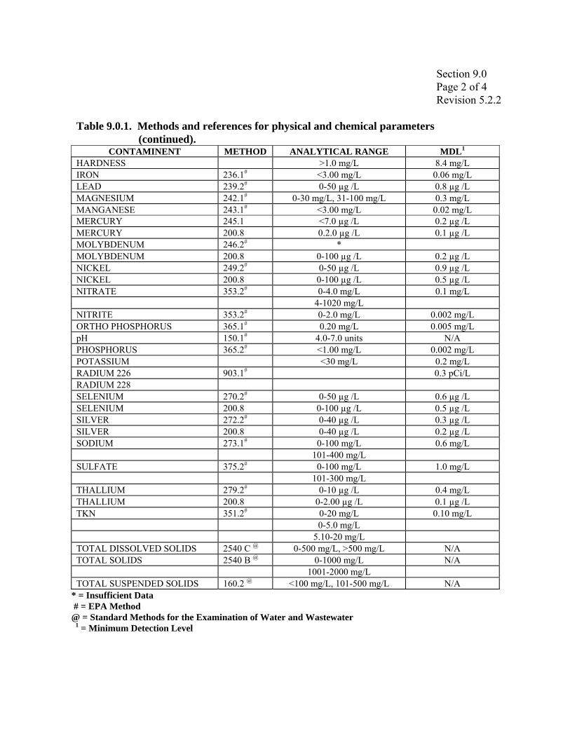
Section 9.0 Page 2 of 4 Revision 5.2.2
Table 9.0.1. Methods and references for physical and chemical parameters
(continued). CONTAMINENT METHOD ANALYTICAL RANGE MDL1
HARDNESS >1.0 mg/L 8.4 mg/L IRON 236.1# <3.00 mg/L 0.06 mg/L LEAD 239.2# 0-50 µg /L 0.8 µg /L MAGNESIUM 242.1# 0-30 mg/L, 31-100 mg/L 0.3 mg/L MANGANESE 243.1# <3.00 mg/L 0.02 mg/L MERCURY 245.1 <7.0 µg /L 0.2 µg /L MERCURY 200.8 0.2.0 µg /L 0.1 µg /L MOLYBDENUM 246.2# * MOLYBDENUM 200.8 0-100 µg /L 0.2 µg /L NICKEL 249.2# 0-50 µg /L 0.9 µg /L NICKEL 200.8 0-100 µg /L 0.5 µg /L NITRATE 353.2# 0-4.0 mg/L 0.1 mg/L 4-1020 mg/L NITRITE 353.2# 0-2.0 mg/L 0.002 mg/L ORTHO PHOSPHORUS 365.1# 0.20 mg/L 0.005 mg/L pH 150.1# 4.0-7.0 units N/A PHOSPHORUS 365.2# <1.00 mg/L 0.002 mg/L POTASSIUM <30 mg/L 0.2 mg/L RADIUM 226 903.1# 0.3 pCi/L RADIUM 228 SELENIUM 270.2# 0-50 µg /L 0.6 µg /L SELENIUM 200.8 0-100 µg /L 0.5 µg /L SILVER 272.2# 0-40 µg /L 0.3 µg /L SILVER 200.8 0-40 µg /L 0.2 µg /L SODIUM 273.1# 0-100 mg/L 0.6 mg/L 101-400 mg/L SULFATE 375.2# 0-100 mg/L 1.0 mg/L 101-300 mg/L THALLIUM 279.2# 0-10 µg /L 0.4 mg/L THALLIUM 200.8 0-2.00 µg /L 0.1 µg /L TKN 351.2# 0-20 mg/L 0.10 mg/L 0-5.0 mg/L 5.10-20 mg/L TOTAL DISSOLVED SOLIDS 2540 C @ 0-500 mg/L, >500 mg/L N/A TOTAL SOLIDS 2540 B @ 0-1000 mg/L N/A 1001-2000 mg/L TOTAL SUSPENDED SOLIDS 160.2 @ <100 mg/L, 101-500 mg/L N/A
* = Insufficient Data # = EPA Method @ = Standard Methods for the Examination of Water and Wastewater
1 = Minimum Detection Level

Section 9.0 Page 3 of 4 Revision 5.2.2
Table 9.0.1. Methods and references for physical and chemical parameters (continued).
CONTAMINENT METHOD ANALYTICAL RANGE MDL1 URANIUM URANIUM 200.8 0-100 µg /L 0.2 µg /L VANADIUM 286.2# * 1.4 µg /L VANADIUM 200.89 0-100 µg /L 0.5 µg /L ZINC 289.1# 0-1000 µg /L 50 µg /L ZINC 200.8# 0-100 µg /L 3.0 µg /L HEXACHLORO-CYCLOPENTADENE 525.2# 0-10 µg /L 0.5 µg /L PROPACHLOR 525.5# 0-10 µg /L 0.5 µg /L HEXACHLOROBENZNE 525.5# 0-10 µg /L 0.5 µg /L SIMAZINE 525.2# 0-10 µg /L 0.5 µg /L ATRAZINE 525.2# 0-10 µg /L 0.5 µg /L LINDANE 525.2# 0-10 µg /L 0.1 µg /L METRIBUZIN 525.2# 0-10 µg /L 0.5 µg /L ALACHLOR 525.2# 0-10 µg /L 0.5 µg /L HEPTACHLOR 525.2# 0-10 µg /L 0.5 µg L METOLACHLOR 525.2# 0-10 µg /L 0.5 µg /L ALDRIN 525.2# 0-10 µg /L 0.5 µg /L HEPTACHLOR EPOXIDE 525.2# 0-10 µg /L 0.1 µg /L CHLORDANE 525.2# 0-10 µg /L 0.5 µg /L BUTACHLOR 525.2# 0-10 µg /L 0.5 µg /L DIELDRIN 525.2# 0-10 µg /L 0.5 µg /L ENDRIN 525.2# 0-10 µg /L 0.5 µg /L BIS-2-ETHYLHEXYL 525.2# 0-10 µg /L 3.0 µg /L ADIPATE 0-10 µg /L METHOXYCHLOR 525.2# 0-10 µg /L 0.5 µg /L BIS-2-ETHYLHEXYL 525.2# 0-10 µg /L 3.0 µg /L PHTHALATE 0-10 µg /L BENZO(A) PYRENE 525.2# 0-10 µg /L 0.2 µg /L ALDICARB SULFOXIDE 521.1# 0-10 µg /L 2.0 µg /L ALDICARB SULFONE 531.1# 0-10 µg /L 1.0 µg /L OXAMYL 531.1# 0-10 µg /L 2.0 µg /L METHOMYL 531.1# 0-10 µg /L 2.0 µg /L 3-HYDROXY-CARBOFURAN 531.1# 0-10 µg /L 2.0 µg /L ALDICARB 531.1# 0-10 µg /L 1.0 µg /L CARBOFURAN 531.1# 0-10 µg /L 2.0 µg /L CARBARYL 531.1# 0.10 µg /L 2.0 µg /L GLYPHOSATE 547# 0-250 µg /L 50 µg /L DIQUAT 549.1# 0-20 µg /L 0.5 µg /L
* = Insufficient Data # = EPA Method @ = Standard Methods for the Examination of Water and Wastewater
1 = Minimum Detection Level

Section 9.0 Page 4 of 4 Revision 5.2.2
Table 9.0.1. Methods and references for physical and chemical parameters (continued).
CONTAMINENT METHOD ANALYTICAL RANGE MDL1 EDB 504# 0-2.0 µg /L 0.05 µg /L DBCP 504# 0-2.0 µg /L 0.2 µg /L ENDOTHALL 548# 0-500 µg /L 50 µg /L DALAPON 515.1# 0-50 µg /L 10 µg /L DICAMBA 515.1# 0-10 µg /L 1.0 µg /L 2,4-D 515.1# 0-10 µg /L 1.0 µg /L PENTA-CHLOROPHENOL 515.1# 0-2.5 µg /L 0.5 µg /L 2,4,5-TP (SILVEX) 515.1# 0-10 µg /L 1.0 µg /L DINOSEB 515.1# 0-10 µg /L 1.0 µg /L PICLORAM 515.1# 0-10 µg /L 1.0 µg /L THM 524.2# 0-20 µg /L 0.5 µg /L 20-80 µg /L 0.5 µg /L VOC 524.2# 0-20 µg /L 0.5 µg /L
* = Insufficient Data # = EPA Method @ = Standard Methods for the Examination of Water and Wastewater
1 = Minimum Detection Level The laboratory routinely analyzes these parameters (Table 9.0.1). Non-routine analyses may also be performed by the laboratory using methodology outlined in the Nineteenth Edition of Standard Methods, within the limitations of laboratory equipment, media, reagents, etc.
The methods noted above are to be used exclusively and an analyst, without prior approval of the section supervisor, may use no other methods.
A. Methods for the Chemical Analysis of Water and Wastes, EPA-600/4-79-020,
Revised March 1983. 1. Methods for the Determination of Metals in Environmental Samples, EPA/600/4-
91/010. 2. Methods for the Determination of Organic Compounds in Drinking Water,
EPA/600/4-88/039, December 1988. 3. Methods for the Determination of Organic Compounds in Drinking Water,
Supplement 1, EPA/600/4-90/020, July 1990. 4. Test Methods for Evaluating Solid Waste, EPA, SW-846, 3rd edition, November
1986. 5. Standard Methods for the Examination of Water and Wastes, 19th edition, 1995.
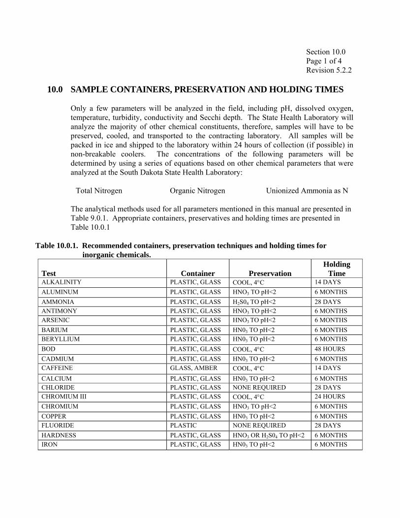
Section 10.0 Page 1 of 4 Revision 5.2.2
10.0 SAMPLE CONTAINERS, PRESERVATION AND HOLDING TIMES
Only a few parameters will be analyzed in the field, including pH, dissolved oxygen, temperature, turbidity, conductivity and Secchi depth. The State Health Laboratory will analyze the majority of other chemical constituents, therefore, samples will have to be preserved, cooled, and transported to the contracting laboratory. All samples will be packed in ice and shipped to the laboratory within 24 hours of collection (if possible) in non-breakable coolers. The concentrations of the following parameters will be determined by using a series of equations based on other chemical parameters that were analyzed at the South Dakota State Health Laboratory:
Total Nitrogen Organic Nitrogen Unionized Ammonia as N
The analytical methods used for all parameters mentioned in this manual are presented in Table 9.0.1. Appropriate containers, preservatives and holding times are presented in Table 10.0.1
Table 10.0.1. Recommended containers, preservation techniques and holding times for
inorganic chemicals.
Test
Container
Preservation Holding
Time ALKALINITY PLASTIC, GLASS COOL, 4°C 14 DAYS ALUMINUM PLASTIC, GLASS HNO3 TO pH<2 6 MONTHS AMMONIA PLASTIC, GLASS H2S04 TO pH<2 28 DAYS ANTIMONY PLASTIC, GLASS HNO3 TO pH<2 6 MONTHS ARSENIC PLASTIC, GLASS HNO3 TO pH<2 6 MONTHS BARIUM PLASTIC, GLASS HN03 TO pH<2 6 MONTHS BERYLLIUM PLASTIC, GLASS HN03 TO pH<2 6 MONTHS BOD PLASTIC, GLASS COOL, 4°C 48 HOURS CADMIUM PLASTIC, GLASS HN03 TO pH<2 6 MONTHS CAFFEINE GLASS, AMBER COOL, 4°C 14 DAYS CALCIUM PLASTIC, GLASS HN03 TO pH<2 6 MONTHS CHLORIDE PLASTIC, GLASS NONE REQUIRED 28 DAYS CHROMIUM III PLASTIC, GLASS COOL, 4°C 24 HOURS CHROMIUM PLASTIC, GLASS HNO3 TO pH<2 6 MONTHS COPPER PLASTIC, GLASS HN03 TO pH<2 6 MONTHS FLUORIDE PLASTIC NONE REQUIRED 28 DAYS HARDNESS PLASTIC, GLASS HNO3 OR H2S04 TO pH<2 6 MONTHS IRON PLASTIC, GLASS HN03 TO pH<2 6 MONTHS
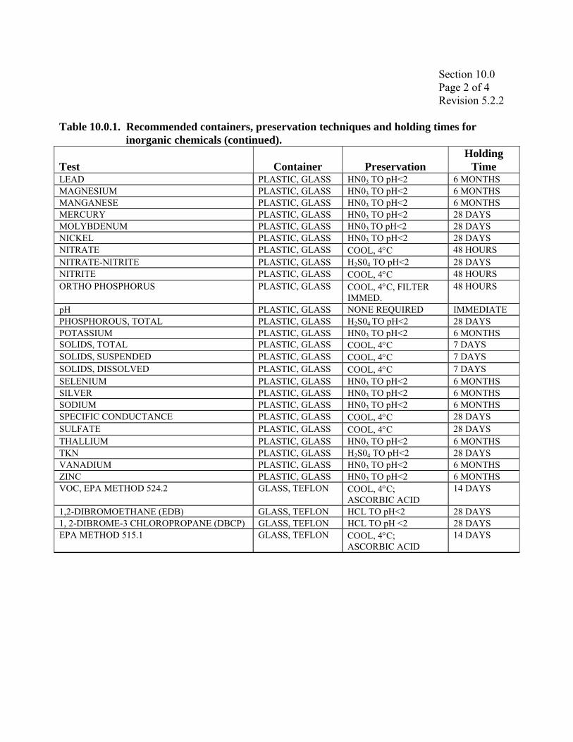
Section 10.0 Page 2 of 4 Revision 5.2.2
Table 10.0.1. Recommended containers, preservation techniques and holding times for
inorganic chemicals (continued). Test
Container
Preservation
Holding Time
LEAD PLASTIC, GLASS HN03 TO pH<2 6 MONTHS MAGNESIUM PLASTIC, GLASS HN03 TO pH<2 6 MONTHS MANGANESE PLASTIC, GLASS HN03 TO pH<2 6 MONTHS MERCURY PLASTIC, GLASS HN03 TO pH<2 28 DAYS MOLYBDENUM PLASTIC, GLASS HN03 TO pH<2 28 DAYS NICKEL PLASTIC, GLASS HN03 TO pH<2 28 DAYS NITRATE PLASTIC, GLASS COOL, 4°C 48 HOURS NITRATE-NITRITE PLASTIC, GLASS H2S04 TO pH<2 28 DAYS NITRITE PLASTIC, GLASS COOL, 4°C 48 HOURS ORTHO PHOSPHORUS PLASTIC, GLASS COOL, 4°C, FILTER
IMMED. 48 HOURS
pH PLASTIC, GLASS NONE REQUIRED IMMEDIATE PHOSPHOROUS, TOTAL PLASTIC, GLASS H2S04 TO pH<2 28 DAYS POTASSIUM PLASTIC, GLASS HN03 TO pH<2 6 MONTHS SOLIDS, TOTAL PLASTIC, GLASS COOL, 4°C 7 DAYS SOLIDS, SUSPENDED PLASTIC, GLASS COOL, 4°C 7 DAYS SOLIDS, DISSOLVED PLASTIC, GLASS COOL, 4°C 7 DAYS SELENIUM PLASTIC, GLASS HN03 TO pH<2 6 MONTHS SILVER PLASTIC, GLASS HN03 TO pH<2 6 MONTHS SODIUM PLASTIC, GLASS HN03 TO pH<2 6 MONTHS SPECIFIC CONDUCTANCE PLASTIC, GLASS COOL, 4°C 28 DAYS SULFATE PLASTIC, GLASS COOL, 4°C 28 DAYS THALLIUM PLASTIC, GLASS HN03 TO pH<2 6 MONTHS TKN PLASTIC, GLASS H2S04 TO pH<2 28 DAYS VANADIUM PLASTIC, GLASS HN03 TO pH<2 6 MONTHS ZINC PLASTIC, GLASS HN03 TO pH<2 6 MONTHS VOC, EPA METHOD 524.2 GLASS, TEFLON COOL, 4°C;
ASCORBIC ACID 14 DAYS
1,2-DIBROMOETHANE (EDB) GLASS, TEFLON HCL TO pH<2 28 DAYS 1, 2-DIBROME-3 CHLOROPROPANE (DBCP) GLASS, TEFLON HCL TO pH <2 28 DAYS EPA METHOD 515.1 GLASS, TEFLON COOL, 4°C;
ASCORBIC ACID 14 DAYS

Section 10.0 Page 3 of 4 Revision 5.2.2
Table 10.0.2. Recommended containers, preservation techniques and holding times for
organic chemicals.
Parameter/Method #
Container
Preservation Holding
Time 2, 4-D GLASS, TEFLON ADJUST pH TO 5-9 14 DAYS 2,4,5-TP GLASS, TEFLON ADJUST pH TO 5-9 14 DAYS DALAPON GLASS, TEFLON ADJUST pH TO 5-9 14 DAYS DINOSEB GLASS, TEFLON ADJUST pH TO 5-9 14 DAYS PICLORAM GLASS, TEFLON ADJUST pH TO 5-9 14 DAYS DICAMBA GLASS, TEFLON ADJUST pH TO 5-9 14 DAYS PENTACHLOROPHENOL GLASS, TEFLON ADJUST pH TO 5-9 14 DAYS EPA METHOD 547 GLASS, TEFLON COOL 4°C 14 DAYS GLYPHOSATE GLASS, TEFLON FROZEN 18 MONTHS EPA METHOD 525 GLASS, TEFLON COOL, 4°C; HCL TO pH<2 7 DAYS ALACHLOR GLASS, TEFLON COOL, 4°C; HCL TO pH<2 7 DAYS ATRAZINE GLASS, TEFLON COOL, 4°C; HCL TO pH<2 7 DAYS BENZO (A) PYRENE GLASS, TEFLON COOL, 4°C; HCL TO pH<2 7 DAYS CHLORDANE GLASS, TEFLON COOL, 4°C; HCL TO pH<2 7 DAYS DI (ETHYLHEXYL) ADIPATE
GLASS, TEFLON COOL, 4°C; HCL TO pH<2 7 DAYS
DI (ETHYLHEXYL) PHTHALATE
GLASS, TEFLON COOL, 4°C; HCL TO pH<2 7 DAYS
ENDRIN GLASS, TEFLON COOL, 4°C; HCL TO pH<2 7 DAYS HEPTACHLOR GLASS, TEFLON COOL, 4°C; HCL TO pH<2 7 DAYS HEPTACHLOR EPOXIDE GLASS, TEFLON COOL, 4°C; HCL TO pH<2 7 DAYS HEXACHLOROBENZENE GLASS, TEFLON COOL, 4°C; HCL TO pH<2 7 DAYS HEXACHLORO-CYCLOPENTADIENE
GLASS, TEFLON COOL, 4°C; HCL TO pH<2 7 DAYS
LINDANE GLASS, TEFLON COOL, 4°C; HCL TO pH<2 7 DAYS METHOXYCHLOR GLASS, TEFLON COOL, 4°C; HCL TO pH<2 7 DAYS SIMAZINE GLASS, TEFLON COOL, 4°C; HCL TO pH<2 7 DAYS TOXAPHENE GLASS, TEFLON COOL, 4°C; HCL TO pH<2 7 DAYS ALDRIN GLASS, TEFLON COOL, 4°C; HCL TO pH<2 7 DAYS BUTACHLOR GLASS, TEFLON COOL, 4°C; HCL TO pH<2 7 DAYS DIELDRIN GLASS, TEFLON COOL, 4°C; HCL TO pH<2 7 DAYS METOLACHLOR GLASS, TEFLON COOL, 4°C; HCL TO pH<2 7 DAYS METRIBUZIN GLASS, TEFLON COOL, 4°C; HCL TO pH<2 7 DAYS PROPOCHLOR GLASS, TEFLON COOL, 4°C; HCL TO pH<2 7 DAYS PCB SCREEN GLASS, TEFLON COOL, 4°C; HCL TO pH<2 7 DAYS EPA METHOD 531.1 GLASS, TEFLON CHLOROACTIC ACID TO pH<3 28 DAYS CARBOFURAN GLASS, TEFLON SODIUM THIOSULFATE 28 DAYS

Section 10.0 Page 4 of 4 Revision 5.2.2
Table 10.0.2. Recommended containers, preservation techniques, and holding times for
organic chemicals (continued).
Parameter/Method#
Container
Preservation Holding
Time OXAMYL GLASS, TEFLON -10°C 28 DAYS 3-HYDROXY CARBOFURAN GLASS, TEFLON -10°C 28 DAYS ALDICARB GLASS, TEFLON -10°C 28 DAYS ALDICARB SULFONE GLASS, TEFLON -10°C 28 DAYS ALDICARB SULFOXIDE GLASS, TEFLON -10°C 28 DAYS CARBARYL GLASS, TEFLON -10°C 28 DAYS METHOMYL GLASS, TEFLON -10°C 28 DAYS EPA METHOD 549 -10°C DIQUAT GLASS, TEFLON COOL 4°C, SODIUM
THIOSULFATE H2S04TO pH<2
A. Sample preservation should be performed immediately upon sample collection.
For composite samples, each aliquot should be preserved at the time of collection. When the use of an automatic sampler makes it impossible to preserve each aliquot, then samples are preserved by maintaining them at 4oC until compositing and sample splitting is completed.
B. Samples should be analyzed as soon as possible after collection. The times listed are the maximum times that samples may be held before analysis and still be considered valid. Samples may be held for longer periods only if the permittee, or monitoring laboratory, has data on file to show that the specific types of samples under study are stable for the longer time.
C. Some samples may not be stable for the maximum time period given in the table. A permittee, or monitoring laboratory, is obligated to hold the sample for a shorter time if knowledge exists to show this is necessary to maintain sample stability.
D. Samples should be filtered immediately on-site before adding preservative for dissolved metals.
E. Guidance applies to samples to be analyzed by GC (Gas Chromatography), LC (Liquid Chromatography) or GC/MS (Gas Chromatography/Mass Spectrometer) for specific organic compounds.

Section 11.0 Page 1 of 1 Revision 5.2.2
11.0 DECONTAMINATION OF SAMPLE CONTAINERS AND SAMPLING
EQUIPMENT
The State Health Lab will decontaminate sample containers prior to use in the field. Decontamination involves detergent washing, rinsing with dilute chromic acid and final rinsing with laboratory-grade distilled water. Decontamination of sampling equipment (probes and instruments) will be accomplished through the use of distilled water.

TRIBUTARY SAMPLING TECHNIQUES

Section 12.0 Page 1 of 21 Revision 5.2.2
12.0 SAMPLING PROCEDURES FOR TRIBUTARY SAMPLING
A. Field Observations
Prior to other activities, comments and observations regarding the weather and sampling site must be recorded. It is important to record all field observations of conditions at the sampling sites that could influence the water quality of the collected sample. These observations are recorded on field data collection sheets (Appendix A). Examples of observations recorded under COMMENTS include: “cloudy, heavy rainfall two days ago, windy, cattle grazing near sampling site, dense submergent or emergent aquatic vegetation present at sampling site.”
In addition to comments, specific observations must be recorded on the field data sheets (METRIC PREFERRED) as follows:
Stage Record in (feet or meters). Discharge Record in (Cubic Feet per Second (CFS) or Cubic Meters per
Second (CMS)). Air Temperature Record in degrees (Fahrenheit or Celsius). Color Describe the color of the water. Dead Fish Record in (Severe, Extreme, Moderate, Mild or None). Film Record in (Severe, Extreme, Moderate, Mild or None). Odor Record in (Severe, Extreme, Moderate, Mild or None). Precipitation Record in (inches or centimeters). Wind Record as (Severe (> 30 MPH), Extreme (20-30 MPH), Moderate
(10-20 MPH), Mild (5-10 MPH) or None (0-5 MPH)). Conductivity Record in (µS/cm-1). Dissolved Oxygen Record in (milligrams per Liter (mg/L). Field pH Record in (su). Water Temperature Record degrees (Fahrenheit or Celsius). Secchi Record in (feet or meters). Sample Depth Record in (feet or meters). Turbidity Record in (Nephelometric Turbidity Units (NTU)). Snow Depth Record in (feet or meters). Ice Cover Record in (Severe, Extreme, Moderate, Mild or None).

Section 12.0 Page 2 of 21 Revision 5.2.2
B. Field Analyses
Calibrate all instruments prior to field use as described in the previous section (Section 6.0). Record all field analysis data on field data collection sheets and in the project notebook.
1. YSI Multi Parameter Meter (650 MDS with Sonde) Method Most projects/studies will use YSI multi parameter meter and must be operated in accordance with manufacturer specifications (Section 6.0). a. Calibrate instrument following Section 6.0. b. Make sure weighted probe guard is attached to the sonde. c. Select Run. d. Place the probe into the stream. e. If water is static, provide stirring by gently and continuously agitating
the probe. f. Allow sufficient time for the sonde and probe to stabilize. g. Record data in logbook and on the data sheet or save in memory. h. When sampling is complete, remove weighted probe guard and
install the calibration cup to protect probes and store unit in carrying case.
2. Dissolved Oxygen Meter (YSI Model 51B Dissolved Oxygen Meter)
a. Calibrate the meter using methods found in Section 6.0 of this manual.
b. Place the probe into the stream and provide stirring. If the probe has no stirrer, gently and continuously agitate the probe.
c. Allow sufficient time for the probe to stabilize to sample temperature and dissolved oxygen.
d. Read and record the temperature. e. Set the Oxygen Solubility Factor dial to “sample temperature.”
Choose the correct position based upon the salinity. f. Read and record the dissolved oxygen. g. Leave the instrument on between sampling sites. Re-check the
calibration at each site. h. Replace batteries after 1000 hours of operation or if the full-scale
adjustment cannot be made.
Section 12.0 Page 3 of 21 Revision 5.2.2
3. pH-Electrode Method
a. Calibrate instrument following Section 6.0 and re-check calibration at each sampling site with pH buffer solution 7.01.
b. Place the electrode into the stream or into a separate, rinsed container with a water sample from the site.
c. Turn on pH meter and allow sufficient time for the readings to stabilize.
d. Read pH. e. Thoroughly rinse the electrode with de-ionized water between
samples and replace probe cover/cap. f. Replace batteries as needed.
4. Temperature
a. Air Temperature
i. Always collect air temperature readings out of direct sunlight (indicate °F or °C, °C preferred).
b. Water Temperature
i. Water temperature should be collected directly from a lake. ii. If a bottle of water needs to be collected to obtain a
temperature, measure the temperature as soon as possible. iii. Place the thermometer into the stream and provide stirring
or gentle agitation. iv. Allow sufficient time for the thermometer to stabilize to
sample temperature. v. Read the temperature (indicate °F or °C, °C preferred).
5. Total Depth a. Record total depth at the maximum cross sectional depth (indicate in
meters) at tributary sites.
Section 12.0 Page 4 of 21 Revision 5.2.2
6. Flow (Marsh-McBirney)
a. Calibrate the meter using methods found in Section 6.0 of this manual.
b. Stake a measuring tape across the stream at the selected site. c. Attach sensor to the bottom of the wading rod (Figure 12.0.1). Point
sensor into the oncoming flow when recording. d. Determine the stream width and choose an interval for measurement
that will give a good cross-sectional area of the stream. Record total water depth at equal intervals across the stream.
e. Once an interval width is chosen, the first reading should be ½ of the chosen interval width. The second and successive readings should be taken at the chosen interval.
f. Record total water depth at the following intervals across the stream.
i. Example, a stream that is 10 meters wide. It is decided that a reading every 2 meters will give a good cross-sectional area of the stream.
ii. The first reading will be one meter (1/2 of 2 meters) away from the bank.
iii. Each of the next four readings will be 2 meters away from the previous recording.
g. To collect a reading, adjust the wading rod so that the sensor is
suspended at 60% of the depth (Figure 12.0.1) at each interval and record flow in ft/sec. Rotate the sensor slightly from side to side and record the highest flow reading.
h. Record velocity in ft/sec at each interval. i. Record all flow data on a discharge measurement field data sheet
(Appendix A). j. If depth is greater than 1.5 meters (5 feet), the flow will have to be
recorded from a depth of 20% and 80% of the total depth in each interval.
k. Use an average of the readings to estimate flow at a given point.

Section 12.0 Page 5 of 21 Revision 5.2.2
Figure 12.0.1. Wading rod for Marsh-McBirney flowmeter. Adapted from the Marsh-
McBirney, Inc. Model 201 portable water flow meter instruction manual.
7. Flow (AquaCalc 5000) a. Connect the AquaCalc to a wading rod or cable reel using the
cable P/N AQ5C-82-2 provided. b. Field-test the instrument to make sure all of the connections are
secure. Select a transect for your test. Start the cups on the current meter spinning and press Measure. The timer will immediately start, and then the counter will start and the mean velocity will be displayed. If, for some reason, the AquaCalc fails to count the revolutions, abort the routine by pressing Enter two times and press Measure again. If the problem continues, refer to the Troubleshooting Section of the operating manual.

Section 12.0 Page 6 of 21 Revision 5.2.2
c. Be sure that the revolutions and counts match. If not, check your
connections for broken wires or insecure couplings. Also check the adjustment of the whisker hair. (A badly corroded or oily whisker hair will cause an audible scratchy sound in the head set, but the AquaCalc will not acknowledge this sound as a good signal).
d. You should now do a “Spin Test” of the current meter to insure its proper operation prior to measurement.
e. Go to the beginning of your transect. On the AquaCalc, select an empty transect and at Station #1 erase all data.
f. Press Set Distance. Either input a Head Stake value of zero or the Tag Line value at the Edge of Water (EOW).
g. Enter the distance read from the tag line corresponding to the starting point of the measurement cross section. Press Set Depth.
h. Enter the depth of the stream. Press Enter. The first depth should always be zero. Note: the AquaCalc will not allow a measurement to be performed at Stations #1 and #99, this ensures a starting and ending point.
i. Once in moving water and the cups are spinning and stable, activate the measurement routine.
j. Press Measure. k. The AquaCalc will immediately start timing, counting the clicks,
and displaying the mean velocity. l. Press Next Station. m. Repeat the previous steps for each station in the transect. n. After completing the measurement at the last station, press Next
Station and enter the EOW location as read on the Tag Line. As with the beginning EOW, this must be input to tell the computer where to stop when summing up the individual transects and calculations.
o. Press Calculate Discharge. p. The AquaCalc will now display “Calculating Discharge.” q. Once calculated, the AquaCalc will then display the Discharge and
Mean Velocity. r. To continue with another measurement, press Go To Transect #
followed by a number from 1 to 9 which corresponds to a new transect location.
s. The AquaCalc is now ready to perform another discharge measurement.

Section 12.0 Page 7 of 21 Revision 5.2.2
8. Stage Recording/Data Logging
a. Program stage recorders and data loggers as per Section 6.0. b. Be sure to check, adjust and download stage recorders and data
loggers every two weeks or as conditions change. c. Keep recorders in dry protected housings.
C. Sample Collection
There are basically two sample collection methods for tributary sampling:
1. Grab sampling 2. Composite sampling (tributary sampling with a suspended sediment sampler)
A typical sample set for a sampling site consists of the following:
1. Two (2) one-liter polypropylene bottles. 2. One (1) 100 ml bottle for total dissolved phosphorus samples. 3. One 250 mL poly-plastic bacteriological bottle.
Note: If sampling protocol requires caffeine analysis: One (1) 1000 ml
amber glass bottle is required. (See Special Sampling Techniques Section 16.0)
4. Collect one (1) extra one-liter sample in a brown polypropylene bottle for use
in filtering the total dissolved phosphorus sample and (if required) algae and chlorophyll-a samples.
Labeling
Waterproof write-on label tape containing the date, time, station identification number, "A" or "B" (one-liter bottles), "C" (250 ml bacteriological bottle), "D" (100 ml bottle for total dissolved phosphorus), surface or bottom and the sampler's name are filled out in waterproof ink and affixed to the appropriate bottles. See the example below.

Section 12.0 Page 8 of 21 Revision 5.2.2
1. Grab Sampling
Collecting a Sample
The "C" bottle (bacteriological sample) should be taken first. Be careful not to contaminate the inside of the lid or mouth of the bottle with your fingers or introduce other sources of contamination. a. The 250 ml bacteriological sample (“C” Bottle)
In no case should composite samples be collected for microbiological examination. i. The "C" bottle should not be rinsed with sampling site
water. ii. Position the open end of the bottle towards the current flow
and away from the hand of the collector. iii. Grasp the bottle securely at the base with one hand and
plunge the bottle down into the water to avoid introducing surface scum.
iv. The sampling depth should be 15.5 cm (6 inches) to 30.5 cm 1 foot) below the water surface if possible. Make a sweeping motion horizontally away from the sampler; if the sampling bottle has a small diameter neck no sweeping action is required.
v. Tip the bottle slightly upward to allow air to escape and the bottle to fill. On the initial plunge, the "C" sample bottle should be filled completely or at least above the 250 mL mark (Figure 12.0.2). Immediately after obtaining the sample, pour off the excess sample water from the container until the sample volume is 250 mL and cap.
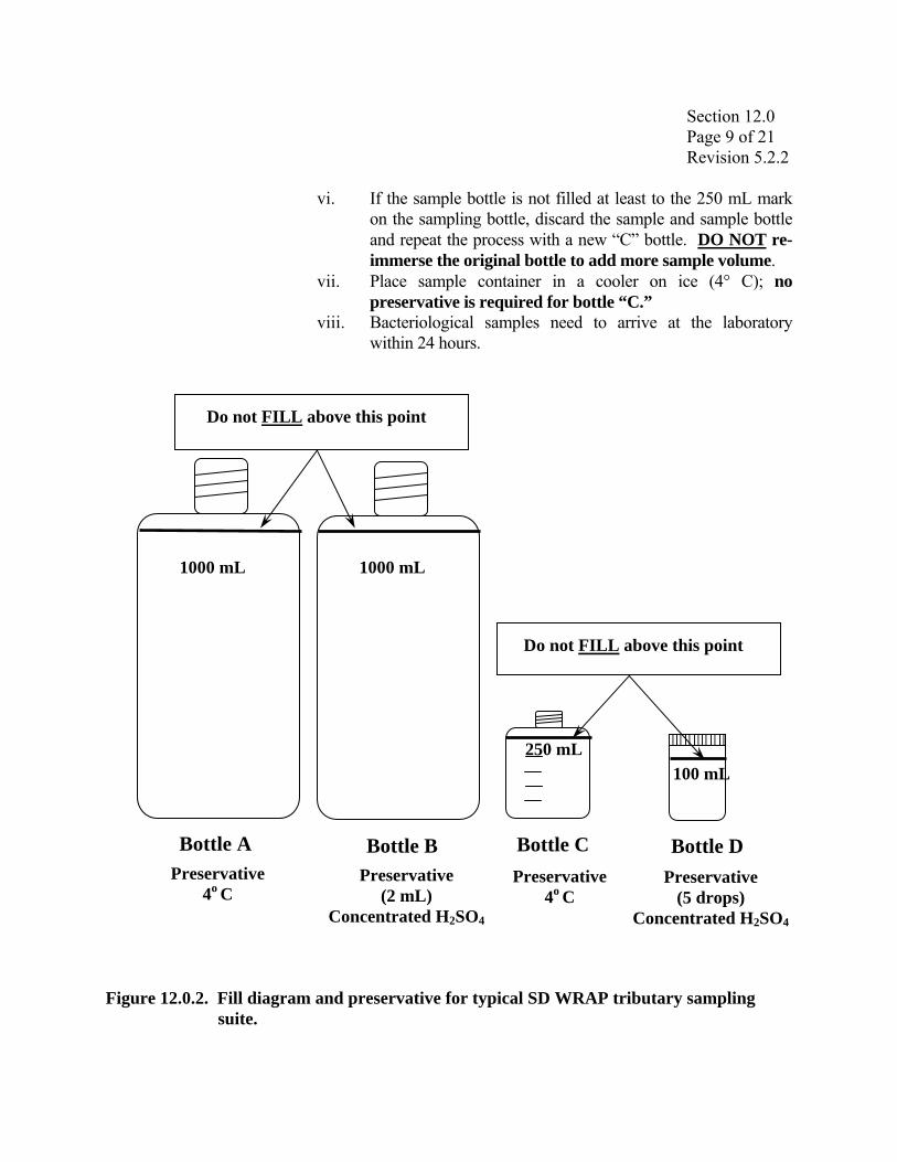
Section 12.0 Page 9 of 21 Revision 5.2.2
vi. If the sample bottle is not filled at least to the 250 mL mark
on the sampling bottle, discard the sample and sample bottle and repeat the process with a new “C” bottle. DO NOT re-immerse the original bottle to add more sample volume.
vii. Place sample container in a cooler on ice (4° C); no preservative is required for bottle “C.”
viii. Bacteriological samples need to arrive at the laboratory within 24 hours.
Figure 12.0.2. Fill diagram and preservative for typical SD WRAP tributary sampling suite.
Do not FILL above this point
Bottle A
1000 mL
Preservative 4o C
Do not FILL above this point
250 mL
Preservative 4o C
Bottle C
1000 mL
Preservative (2 mL)
Concentrated H2SO4
Bottle B
100 mL
Preservative (5 drops)
Concentrated H2SO4
Bottle D

Section 12.0 Page 10 of 21 Revision 5.2.2
b. The "A" bottle (one-liter bottle)
Because of the small diameter of the neck of the bottle, no sweeping motion is required while filling the bottle “A.” Fill the “A” bottle following the procedure below.
i. The "A" bottle and cap should be rinsed with sampling site
water prior to collection of the sample to ensure no contamination.
ii. Position the open end of the bottle towards the current flow and away from the hand of the collector.
iii. Grasp the bottle securely at the base with one hand and plunge the bottle down into the water to avoid introducing surface scum. The sampling depth should be 15.5 cm (6 inches) to 31.5 cm (1 foot) below the water surface, if possible.
iv. Tip the bottle slightly upward to allow air to escape and the bottle to fill.
v. The "A" sample bottle should be filled completely or filled at least above the volume indicated in Figure 12.0.2. Immediately after obtaining the sample, pour off the excess sample water from the container until the sample volume complies with Figure 12.0.2 and cap immediately.
vi. Place sample container in a cooler on ice (4° C), no preservative is required for bottle “A.”
c. The "B" bottle (one-liter bottle)
Follow collection procedures for filling bottle “A” to fill bottle "B." Preserve the sample using the following procedure below.
i. After the sample has been collected, preserve this sample with
2 ml of concentrated sulfuric acid (H2SO4) to lower the pH of the sample below 2 standard units.
ii. After H2SO4 has been added, the sample bottle is inverted several times to ensure mixing of the preservative throughout the sample.
iii. Place sample container in a cooler on ice (4° C) for shipment to the laboratory.

Section 12.0 Page 11 of 21 Revision 5.2.2
d. Collection of extra one liter bottle
If collecting only total dissolved phosphorus water to be filtered, the sample can be collected in a one-liter polypropylene bottle. If, however, chlorophyll a and/or algae samples are also required, collect the sample in a one-liter brown polypropylene bottle and fill following collection procedures for filling bottle “A.” If chlorophyll-a and/or algae samples are not required, discard the rest of the sample after filtering for the total dissolved phosphorus sample.
e. The "D" bottle (100 mL plastic bottle (“X” top))
Water to be filtered for this sample comes from the extra one-liter bottle collected in Section 12.0 (B.) (1.) (d.). Procedure for field filtration and preservation of the total dissolved phosphorus sample are described below.
i. Thoroughly rinse the “D” bottle and cap with de-ionized
(distilled) water. ii Thoroughly rinse the field filtration device with de-ionized
(distilled) water prior to assembly, once rinsed, assemble the field filtration device with a new filter (47 mm diameter, 0.45 micron pore size filter) and vacuum (filter/rinse) approximately 250 ml of distilled water through the filter (Figure 12.0.3).
iii. After vacuum filtration, empty the distilled water from the bottom reservoir, by removing both the cap and the hose from the bottom reservoir and pouring the water out of one of the holes. DO NOT remove the upper chamber during the rinsing operation.
iv. Pour approximately 120 mL of sample water (from the extra one-liter bottle) into the upper chamber and filter. If the filter clogs due to excessive amounts of suspended sediment, see step v. below.
v. If 100 mL cannot be filtered at one time because of excessive suspended solids, pour the portion of filtered water in the bottom reservoir into the “D” bottle and cap, then remove the clogged filter, and repeat the process above (i., ii., iii. and iv.).
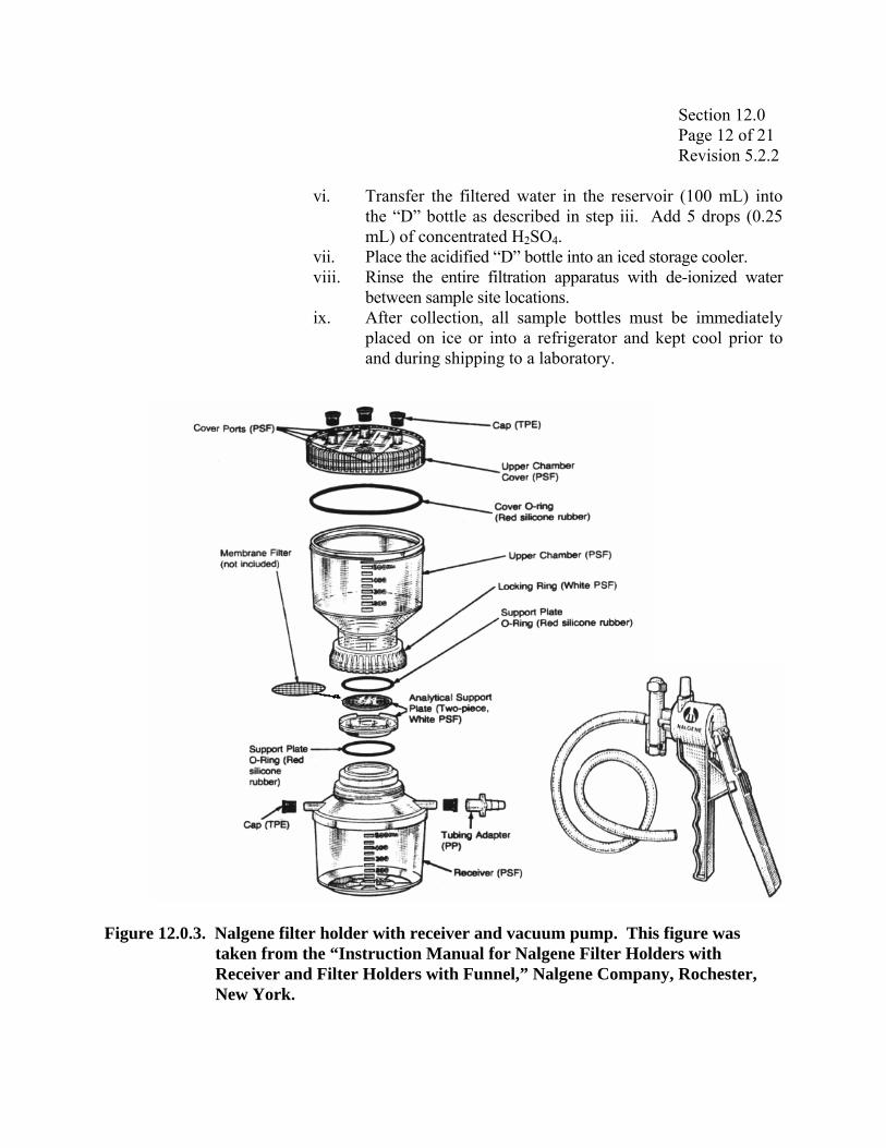
Section 12.0 Page 12 of 21 Revision 5.2.2
vi. Transfer the filtered water in the reservoir (100 mL) into
the “D” bottle as described in step iii. Add 5 drops (0.25 mL) of concentrated H2SO4.
vii. Place the acidified “D” bottle into an iced storage cooler. viii. Rinse the entire filtration apparatus with de-ionized water
between sample site locations. ix. After collection, all sample bottles must be immediately
placed on ice or into a refrigerator and kept cool prior to and during shipping to a laboratory.
Figure 12.0.3. Nalgene filter holder with receiver and vacuum pump. This figure was
taken from the “Instruction Manual for Nalgene Filter Holders with Receiver and Filter Holders with Funnel,” Nalgene Company, Rochester, New York.
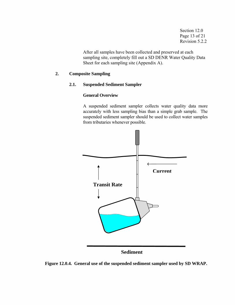
Section 12.0 Page 13 of 21 Revision 5.2.2
After all samples have been collected and preserved at each sampling site, completely fill out a SD DENR Water Quality Data Sheet for each sampling site (Appendix A).
2. Composite Sampling
2.1. Suspended Sediment Sampler
General Overview A suspended sediment sampler collects water quality data more accurately with less sampling bias than a simple grab sample. The suspended sediment sampler should be used to collect water samples from tributaries whenever possible.
Figure 12.0.4. General use of the suspended sediment sampler used by SD WRAP.
Current
Transit Rate
Sediment

Section 12.0 Page 14 of 21 Revision 5.2.2
The suspended sediment sampler is comprised of a US DH-81A adapter, US DH-77 plastic cap, US DH-77 plastic nozzle, US DH-77 three (3) liter plastic bottle and a three (3) foot wading rod with handle. The “transit rate” of the suspended sediment sampler is the rate of movement of the suspended sediment sampler from the surface of the stream to the bottom of the stream and back again to the surface (Figure 12.0.4). This rate must be constant at all sampling verticals at every sampling station, i.e. the rate of movement must be the same at each sampling interval. The transit rate also needs to be fast enough so that it does not allow the collection bottle to over-fill.
a. The sampling bottle(s) should not be filled to more than 90%
capacity. b. A separate bottle or container should be on hand to hold the
sample until a sufficient amount of water is collected to fill the needed sample bottles.
c. A 0.91-meter (3-foot) wading rod is provided with the suspended sediment sampler bottle. If the stream depth is too deep for this wading rod then it will be necessary to attach an extension pole to the wading rod.
When to use the Suspended Sediment Sampler
The sampler is best used at depths greater than 0.30 meter (1 foot). If the field technician should encounter low flow (< 0.06 cms (2.0 cfs)) or shallow depth (< 0.30 m (1 foot) situation at the tributary sampling location, then the Grab Sampling methods described previously ((B), (1) of this section) should be employed. Suspended sediment sampler

Section 12.0 Page 15 of 21 Revision 5.2.2
a. Suspended Sediment Sampling Procedure
i. The sediment sampler and a bottle for compositing the water sample should be rinsed with sample water prior to use at each site and rinsed with de-ionized water after use at each site. The pre-rinse should be with sampling water from the tributary site to be sampled. Distilled water should be used to rinse the sampler and bottle after the sample is collected at the site.
ii. Stake a tape measure across the stream at the sampling station (transect).
iii. Attach the suspended sediment sampler to the bottom of the wading rod. Facing upstream, point the nozzle into the oncoming flow when collecting the sample (Figure 12.0.4).
iv. The suspended sediment sampler should be used at the same intervals from which the flow data was collected. If flow data was collected every 0.15 meter (0.5 foot) then the sediment sampler should be used at every 0.15 meter (0.5 foot) interval.
v. The sampler nozzle should be lowered to just above the water’s surface, allowing the back end of the sampler to rest on the surface of the water. This will allow proper orientation of the sampling bottle with respect to flow.
vi. The sediment sampler is gently moved downward until the tail end of the bottle all most touches the streambed. Once the sampler touches reaches this point, the direction is immediately reversed, returning the bottle to the surface. The sampler must be moved at a constant transit rate throughout this entire sequence (see General Overview paragraph).
vii. Once the sampler has returned to the surface, move to the next interval in the stream, or empty the sample into the composite container if you cannot complete one more up-and-down cycle without exceeding the sample bottle’s 80% full mark.

Section 12.0 Page 16 of 21 Revision 5.2.2
viii. Move to the next interval and use the exact same
transit rate (upward and downward movement of the sample bottle) explained above.
ix. Note: The movement, either upward or downward, must be conducted at a constant rate at each interval. Also, the transit rate should be such that it does not allow the water bottle to overfill.
x. Once the last vertical sample has been collected, the field sampler must determine if the volume of water in the composite sample bottle is enough to fill all the sample bottles (bottles A, B, D and extra one-liter sampling bottle) including any special samples such as pesticides or any quality assurance/quality control samples. If the volume of water in the composite bottle is sufficient after the first series of verticals, the collection period ends. If there is not enough water to fill all the necessary sampling bottles, another round of vertical sampling must be completed.
xi. Note: If the volume of water collected is not enough to fill all the bottles, all vertical sampling points must be sampled again. Samples must be collected across the entire stream cross-section so that a representative (integrated/composite) sample has been collected.
xii. After a sufficient composite sample has been collected, bottles must then be filled (A, B, and D). The C bottle (fecal coliform) is filled by dipping the bottle in the stream as described in (Section 12.0 (1.) (a.), page 8).
xiii. Prior to filling each sample bottle, it is necessary to stir, invert or mix the composite bottle so that the chemistry and sediment particles are uniform throughout the composite bottle.
xiv. After stirring, fill bottle A, stir, fill bottle B, then to fill bottle D, remove the necessary amount of sample into the rinsed Nalgene Vacuum Pump container. Filter this and put it into bottle D using the bottle “D” filtration method described in Section 12.0 (1.) (e.), page 11.

Section 12.0 Page 17 of 21 Revision 5.2.2
xv. Preserve the sample with 5 drops (0.25 ml) of
concentrated H2SO4, label, fill out SD DENR Water Quality Data Sheets, package (sample cooler on ice) and ship to the contracting laboratory.
B. Chlorophyll a Sampling
Procedure for Tributary Chlorophyll a Sampling
Generally, tributary chlorophyll a sampling consists of three discrete sub-samples that are composited into one along a transect in a stream or river. Individual/discrete samples will consist of one grab sample each. Select a wadeable area upstream of the sampling site (chemical or bioassessment) and set up a transect. Composite samples will be collected in three (3) pre-rinsed 500 ml brown (opaque) sampling bottles and composited into one. The samples should be kept out of the sun and on ice. Rinse these bottles thoroughly with de-ionized water prior to use. For individual/discrete samples use a separate pre-rinsed 500 ml brown (opaque) sampling bottle for every site. 1. For composite samples, collect three 500 ml grab samples, one along the
transect near the stream bank (collect samples only from areas with noticeable flow), one from mid-transect and one along the transect near the far stream bank.
2. For individual/discrete samples collect the sample from mid-transect. Fill the sample bottle(s) using the method described below.
a. Position the open end of the bottle (500 ml brown bottle) towards the
current flow and away from the hand of the collector. b. Grasp the bottle securely at the base with one hand and plunge the
bottle down into the water to avoid introducing surface scum. c. The sampling depth should be 15 cm (0.5 foot) to 30.5 cm (1 foot)
below the water surface if possible. If the waterbody is static, make a sweeping motion horizontally away from the sampler.

Section 12.0 Page 18 of 21 Revision 5.2.2
d. Tip the bottle slightly upward to allow air to escape and the bottle to
fill. The sample bottle should be filled to within approximately one inch of the top to allow mixing of the sample before analysis.
3. Take the sample(s) back to shore to conduct sub-sample compositing and/or
filtration. All compositing and filtration will take place in a shaded area out of direct sunlight using the same filter apparatus in Figure 12.0.3.
4. For individual/discrete samples, follow filtration procedures described in “7” and following.
5. For composite samples, pour 166 ml of water from each 500 ml sub-sample bottle into a graduated cylinder and pour contents into a brown composite bottle.
6. A minimum of 400 ml of sample water will be needed to complete chlorophyll a filtering (composite sample or discrete). Note: the project officer will determine the minimum amount of sample water to be filtered, for all projects a minimum of 400 ml is needed. Gently mix, invert or shake the sample bottle before pouring the sample into the filter apparatus.
7. Thoroughly rinse the field filtration device with de-ionized (distilled) water prior to assembly, once rinsed assemble the field filtration device with a new filter (47 mm diameter, 1.0 micron glass fiber filter (Note that these filters are different than the 0.45 micron membrane filters used for total dissolved phosphorus filtration) (Figure 12.0.3).
8. Vacuum filter/rinse approximately 250 ml of distilled water through the filter.
9. Using a graduated cylinder, pour a minimum of exactly 400 ml of sample water into the upper chamber. Pump the vacuum pump gently as not to break algal cells (approximately 10 inches of Hg (259 mm Hg or 5 lbs/in2)).
10. If the upper and lower chambers of the filter apparatus have a maximum capacity of 250 ml, filter 200 ml of the sample, then pour the filtered water out on to the ground. Once the lower reservoir is empty, add the final 200 ml to the upper chamber and finish the filtering process.
11. If the sample is very turbid or contains excessive amounts of algae or solids, add the appropriate (known volume) amount of water to the upper chamber (400 ml or 200 ml) and filter as much of the sample as possible (until no water will go through the filter). Carefully pour the remaining contents of the upper chamber into a graduated cylinder and record the volume. Subtract the remaining volume from the initial volume to determine total volume filtered. Record this on the label (step 15)).

Section 12.0 Page 19 of 21 Revision 5.2.2
12. After filtering (total volume or 400 ml), gently remove the upper chamber
and, with tweezers, fold the side of the filter with the deposited algae over onto itself once. Then fold the filter one more time into a triangle shape (quartered) trapping the algae on the inside of the filter.
13. With tweezers, place the folded filter on a piece of aluminum foil. 14. Securely wrap the filter paper in aluminum foil, making sure no sunlight
can reach the filter. 15. Label the aluminum foil with the date, time, site, tributary name (project
name), sampler initials and the volume of water filtered (VERY IMPORTANT). See below: Secure the label to the aluminum foil with clear packing tape.
16. Place the aluminum foil with the chlorophyll a sample into a zip-lock freezer bag. Keep the filter as close to freezing temperature as possible during transportation. As soon as possible, freeze the filter and keep it frozen until laboratory analysis is conducted.
17. Sample holding time for chlorophyll a is 3 WEEKS, send in all frozen chlorophyll a samples as soon as possible to the address below. Call project officer immediately after sample collection to coordinate sample analysis.
18. Frozen chlorophyll a samples should be sent to the South Dakota Public Health Laboratory in the same cooler as chemical samples, at the address below:
South Dakota Public Health Laboratory 615 East Fourth Street Pierre, South Dakota 57501-1700
Site # Lake Name (Project Name) Sampler Initials
Chlorophyll-a
Date ml of sample filtered Time

Section 12.0 Page 20 of 21 Revision 5.2.2
C. Shipping the Sample
General Samples
1. Completely fill out a SD DENR Water Quality Data Sheet (Appendix A) for each site/station/sample in the cooler (including chlorophyll a samples).
2. All sample containers (bottles and chlorophyll a samples) are placed in a large plastic bag. Seal/tie the plastic bag and place the plastic bag with the samples into a shipping cooler.
3. Ice will be placed in two heavy plastic bags, which is then placed in the cooler with the samples.
4. Make sure that all SD DENR Water Quality Data Sheets (Appendix A) are filled out completely (one sample sheet for each sampling site in the cooler). These documents are placed inside the cooler between the insulation and cardboard lid.
5. Securely seal the cooler with clear packing tape. 6. Coolers are shipped or taken by the sampler to the State Health Laboratory at
the address below or other contracted laboratory where analyses are performed.
South Dakota Public Health Laboratory 615 East Fourth Street Pierre, South Dakota 57501-1700
Chain-of-Custody Samples
1. Completely fill out a SD DENR Water Quality Data Sheet (Appendix A) for each site/station/sample in the cooler. The SD DENR Water Quality Data Sheet also serves the chain-of-custody document which documents/identifies all samples in the cooler (including chlorophyll a samples).
2. All sample containers (bottles and chlorophyll a samples) are placed in a large plastic bag. Sign, date and write the word “SEALED” on a chain-of-custody seal. Seal the plastic bag with a chain-of-custody seal and place a strip of clear packing tape around seal. Place the plastic bag with the samples into a shipping cooler.

Section 12.0 Page 21 of 21 Revision 5.2.2
3. Ice will be placed in a heavy plastic bag, which is then placed in the cooler
with the samples. 4. Make sure that all SD DENR Water Quality Data Sheets (Appendix A) are
filled out completely (one sample sheet for each sampling site in the cooler). 5. Sign and fill in date and time in the Lab Comments section of the SD DENR
Water Quality Data Sheets to complete chain-of-custody. 6. Retain one copy of each of the SD DENR Water Quality Data Sheets (chain-
of-custody record), and send the original copies with the samples. Place all remaining copies of the SD DENR Water Quality Data Sheets inside the cooler between the insulation and cardboard lid.
7. Securely seal the cooler with clear packing tape. 8. Coolers are shipped or taken by the sampler to the State Health Laboratory at
the address below or other contracted laboratory where analyses are performed.
South Dakota Public Health Laboratory 615 East Fourth Street Pierre, South Dakota 57501-1700

Section 13.0 Page 1 of 2 Revision 5.2.2
13.0. WATERSHED MODELING
A. Agricultural Non-Point Source (AGNPS) and Annualized Agricultural Non-Point Source (AnnAGNPS) Watershed Models
Overview Agricultural NonPoint Source Pollution Model (AGNPS) is a computer simulation model developed to analyze the water quality of runoff from watersheds. The model predicts runoff volume and peak rate, eroded and delivered sediment, nitrogen, phosphorus and chemical oxygen demand concentrations in the runoff, and the sediment for a single storm event for all points in the watershed. Proceeding from the headwaters to the outlet, the pollutants are routed in a step-wise fashion so the flow at any one point may be examined. AGNPS is intended to be used as a tool to objectively evaluate the water quality of the runoff from agricultural watersheds and to present a means of objectively comparing different watersheds throughout the state. SD DENR also uses the Annualized NonPoint Source Pollution Model (AnnAGNPS), an updated Windows version of AGNPS. AnnAGNPS runs within ArcView 3.2® and utilizes Global Information System (GIS) layers (soils, land use, etc.) to estimate sediment and nutrient loading from a selected watershed. AnnAGNPS also incorporates feedlot information in modeling the watershed. The AnnAGNPS model has a utility (CONCEPTS) to analyze channel and streambank erosion.
B. Pacific Southwest Interagency Committee (PSIAC) Sediment Evaluation Method
Overview The PSIAC sediment evaluation model is used to determine sediment loadings in watersheds that are composed of greater than 50 percent grass/rangeland. The watershed evaluation is done using a multidisciplinary team composed of local and regional NRCS personnel, staff from Water Resource Assistance Program and local coordinators. The South Dakota State Office of NRCS produces the reports. PSIAC modeling can be used to compare subwatersheds; however, PSIAC does not give a field-by-field comparison of erosional problems.
Section 13.0 Page 2 of 2 Revision 5.2.2
C. FLUX Model
Overview Flux is an interactive program designed for use in estimating the loading of nutrients or other water quality components passing a tributary sampling site over a given period of time. These estimates can be used in formulating reservoir nutrient balances over annual or seasonal averaging periods appropriate for application of empirical eutrophication models. Data requirements include (a) grab sample nutrient concentrations, typically measured at a weekly to monthly frequency for a period of at least a year, (b) corresponding flow measurements (instantaneous or daily mean values) and (c) a complete flow record (mean daily flows) for the period of interest.
IN-LAKE SAMPLING TECHNIQUES

Section 14.0 Page 1 of 21 Revision 5.2.2
14.0 IN-LAKE SAMPLING PROCEDURES
A. Field Observations
Prior to other activities, comments and observations regarding the weather and sampling site must be recorded. It is important to record all field observations of conditions at the sampling sites that could influence the water quality of the collected sample. These observations are recorded on field data collection sheets (Appendix A). Examples of observations recorded under “Comments” include: “cloudy, heavy rainfall two days ago, windy, cattle grazing in or around the lake, dense submergent or emergent aquatic vegetation present at sampling site”, etc.
In addition to comments, specific observations must be recorded on the field data sheets (METRIC PREFERRED) as follows:
Air Temperature Record in degrees (Fahrenheit or Celsius). Color Describe the color of the water. Dead Fish Record in (Severe, Extreme, Moderate, Mild or None). Film Record in (Severe, Extreme, Moderate, Mild or None). Odor Record in (Severe, Extreme, Moderate, Mild or None). Precipitation Record in (inches or centimeters). Wind Record as (Severe (> 30 MPH), Extreme (20-30 MPH), Moderate
(10-20 MPN), Mild (5-10 MPN) or None (0-5 MPN)). Conductivity Record in (µS/cm). Dissolved Oxygen Record in (milligrams per Liter (mg/L). Field pH Record in (su). Water Temperature Record degrees (Fahrenheit or Celsius). Secchi Record in (feet or meters). Sample Depth Record in (feet or meters). Turbidity Record in (Nephelometric Turbidity Units (NTU)). Snow Depth Record in (feet or meters). Ice Cover Record in (Severe, Extreme, Moderate, Mild or None).

Section 14.0 Page 2 of 21 Revision 5.2.2
B. Field Analyses
Calibrate all instruments prior to field use as described in the Section 6.0). Record all field analysis data on field data collection sheets and in the project logbook.
1. YSI Multi Parameter Meter (650 MDS with Sonde) Method Most projects/studies will use YSI multi-parameter meter and must be operated in accordance with manufacturer specifications (Section 6.0). a. Calibrate instrument following Section 6.0 and record all calibration
values on the South Dakota YSI Calibration Worksheet (Appendix A).
b. Make sure weighted probe guard is attached to the sonde. c. Select Run. d. Place the probe into the lake. e. If water is static, provide stirring by gently and continuously agitating
the probe. f. Allow sufficient time for the sonde and probe to stabilize. g. Record data in logbook and on a data sheet or save in memory. h. A procedure for saving data in memory storage using the 650 MDS is
given below. Parameter profiles (surface, every one (1) meter and the bottom) should be collected at each in-lake sampling site location and are as follows. a. Power up the YSI 650 MDS and connect the sonde. b. Calibrate the sonde following steps in Section 6.0 (F) c. Move out to sampling site and deploy sonde (surface sample). d. Select Logging Setup. e. Make sure the Use Site List is not checked. If checked, highlight use
site list and select Enter to deactivate the selection. f. Press Esc to return to main menu. g. Select Sonde Run. h. When the parameters have stabilized, highlight the log one sample in
the box above the parameter list and press Enter. i. The user will be prompted to enter a file name and site description. j. Enter file name (i.e. Smith1). k. Enter site description (i.e. Smith Lake).

Section 14.0 Page 3 of 21 Revision 5.2.2
l. Press OK. m. Press Enter to log sample information in 650 memory (sample
logged will show in the display box). n. Lower sonde down to one meter and let the parameters stabilize,
highlight log one sample and press Enter. o. Continue this procedure until the profile is completed ((every meter
until the bottom is reached (just above the bottom e.g. 0.5 meters). p. When the profile is complete press Esc to return to main menu. q. View the file just created to ensure data was collected and logged
correctly. r. Select File. s. Select View File. t. When sampling is complete, remove weighted probe guard and
install the calibration cup to protect probes and store unit in carrying case.
2. Dissolved Oxygen Meter (YSI Model 51B Dissolved Oxygen Meter)
Parameter profiles (surface, every one (1) meter and the bottom) should be collected at each in-lake sampling site location a. Attach the 7.62 meter (25-foot) cable to YSI 51B meter. b. Calibrate the meter using methods found in Section 6.0 of this
manual. c. Place the probe into the lake just below the surface of the water and
provide stirring. If the probe has no stirrer, gently and continuously agitate the probe.
d. Allow sufficient time for the probe to stabilize to sample temperature and dissolved oxygen.
e. Read and record the temperature. f. Set the Oxygen Solubility Factor dial to “sample temperature.”
Choose the correct position based upon the salinity. g. Read and record the dissolved oxygen. h. Continue this procedure until the profile is completed (every meter
until the bottom is reached. i. Leave the instrument on between sampling sites. Re-check the
calibration at each site. j. Replace batteries after 1000 hours of operation or if the full-scale
adjustment cannot be made.

Section 14.0 Page 4 of 21 Revision 5.2.2
3. Temperature
a. Air Temperature
Always collect air temperature readings out of direct sunlight (indicate °F or °C, °C preferred).
b. Water Temperature
i. Water temperature should be collected directly from the lake. ii. If a bottle of water needs to be collected to obtain a
temperature, measure the temperature as soon as possible. iii. Place the thermometer into the lake and provide stirring or
gentle agitation. iv. Allow sufficient time for the thermometer to stabilize to
sample temperature. v. Read the temperature (indicate °F or °C, °C preferred).
4. Dissolved Oxygen/Temperature Profiles
a. At lake sites, collect profiles of temperature and dissolved oxygen for every 1 meter of depth, starting just below the surface and ending approximately 0.3 meters off the bottom.
b. Record depth, temperature, and dissolved oxygen on In-lake Field Data Collection Sheet (Appendix A) and log to YSI 650 MDS meter.
5. pH-Electrode Method
a. Calibrate instrument following Section 6.0 and re-check calibration at each sampling site with pH buffer solution 7.01.
b. Place the electrode into the lake just below the surface of the water or into a separate, rinsed container with sample water from the site.
c. Turn on pH meter and allow sufficient time for the readings to stabilize.
d. Read pH. e. Thoroughly rinse the electrode with de-ionized water between
samples and replace probe cover/cap. f. Replace batteries as needed.

Section 14.0 Page 5 of 21 Revision 5.2.2
6. Secchi Depth
a. Lower the Secchi disk with calibrated rope into the lake from the shaded side of the boat.
b. Drop the Secchi down until it is no longer visible. c. Bring the Secchi up until you can just barely make out the cross
pattern. d. Record the depth of the Secchi Disk in meters on the In-lake Field
Data Collection Sheet (Appendix A). e. Repeat the above procedure and average the two readings for the
final Secchi depth reading.
7. Total Depth a. Record total depth at all lake sites (in meters) on the In-lake Field
Data Collection Sheet (Appendix A).
C. In-lake Water Sampling Method (Van Dorn-type sampler)
Messenger
Catch
Tripping Lever
Plunger
Cable andLoop
Figure 14.0.1. Van Dorn-type sampler. (Wildlife Supply Company – Alpha Bottle)
Section 14.0 Page 6 of 21 Revision 5.2.2
Most in-lake water samples, both grab and composite, will be collected using a Van Dorn sampler (Figure 14.0.1). Both surface and bottom samples will be collected using this method.
Sampler Setup Procedure
Rinse the sampling apparatus thoroughly with water from the sampling site prior to collection of samples. Surface samples should be collected approximately 1 meter (3.3 feet) below the surface of the water. Bottom samples should be collected from 0.5 meter (1.6 feet) above the lake bottom. Care must be taken not to come in contact with the lake bottom, as this may result in suspended bottom sediment in the sampler. The SD DENR WRAP uses two styles of Van Dorn samplers. Both setup procedures are provided below. Trip Lever Style (older style, Figure 14.0.1) a. Place the sampler catch behind the tripping lever. b. Pull one of the plungers from one end of the sampler and clip the cable
loop of the plunger to the appropriate sampler catch. If placed properly, the plunger and cable will put pressure (torque) on the sampler catch and tripping lever.
c. Pull the plunger and cable from the opposite end and hook the loop appropriately to the sampler catch. The Van Dorn sampler is now ready to be used to collect a water sample.
d. Lower the sampler into the water and stop the sampler at the appropriate depth. Send the messenger (Figure 14.0 1) down the line to trip the sampler.
e. Pull the filled sampler up from the lake. When the bottom sample is collected, check for an excessive amount of bottom sediment or turbidity. If the sample appears turbid, discard the sample and repeat steps a through e.
f. Once the sample is acquired, fill the sample bottles appropriately. g. Before lengthy storage, rinse the Van Dorn sampler with distilled water.
Pin Release Style (newer style, not shown) a. Make sure the pin mechanism is in good working order. b. Press down the pin release and pull plunger from the end nearest the trip
release and hook the cable loop of the plunger into the appropriate slot in the pin release mechanism.
Section 14.0 Page 7 of 21 Revision 5.2.2
c. Release the pin release and ensure the cable loop is completely around the
pin (not pinched by the pin). d. Pull the plunger and cable from the opposite end and hook the cable loop to
the opposite pin on the pin release. The Van Dorn sampler is now ready to be used to collect a water sample.
e. Lower the sampler into the water and stop the sampler at the appropriate depth. Send the messenger down the line to trip the sampler.
f. Pull the filled sampler up from the lake. When the bottom sample is collected, check for an excessive amount of bottom sediment or turbidity. If the sample appears turbid, discard the sample and repeat steps b through f.
g. Once the sample is acquired, fill the sample bottles appropriately. h. Before lengthy storage, rinse the Van Dorn sampler with distilled water.
D. In-lake Sample Collection
There are basically two sample collection methods for in lake sampling:
1. Grab sampling (both with (1.2) and without (1.1) the use of a Van Dorn-type sampler).
2. Composite sampling (in-lake sampling with a Van Dorn-type sampler).
A typical sample set for a sampling site consists of the following:
1. Two (2) one-liter polypropylene bottles. 2. One (1) 100 ml bottle for total dissolved phosphorus samples. 3. One 250 mL poly-plastic bacteriological bottle.
Note: If sampling protocol requires caffeine analysis: One (1) 1000 ml
amber glass bottle is required. (See Special Sampling Techniques Section 16.0)
4. Collect two (2) extra one-liter samples (one for surface and one for bottom*
samples) in brown polypropylene bottle for use in filtering the total dissolved phosphorus, chlorophyll-a sample and, if required, algae samples.
* Bottom samples will not be collected if the total water depth of the site is less
than 2.74 meters (9 feet) or is outlined in the sampling plan.

Section 14.0 Page 8 of 21 Revision 5.2.2
Labeling
Waterproof write-on label tape containing the date, time, station identification number, "A" or "B" (one-liter bottles), "C" (250 ml bacteriological bottle), "D" (100 ml bottle for total dissolved phosphorus), surface or bottom and the sampler's name are filled out in waterproof ink and affixed to the appropriate bottles. See the example below.
1. Grab Sampling
1.1. Collecting a Sample (without the use of a Van Dorn-type sampler)
The following section describes the procedure for collecting an in-lake grab sample (surface) without the use of a Van Dorn-type sampler. The "C" bottle (bacteriological sample) should be taken first. Be careful not to contaminate the inside of the lid or mouth of the bottle with your fingers or introduce other sources of contamination. a. The 250 ml bacteriological sample (“C” Bottle)
Composite samples WILL NOT BE collected for microbiological examination. i. The "C" bottle should not be rinsed with sampling site
water. ii. Position the open end of the bottle away from the hand of the
collector, the shore, the sampling platform, or boat. iii. Grasp the bottle securely at the base with one hand and
plunge the bottle down into the water to avoid introducing surface scum.

Section 14.0 Page 9 of 21 Revision 5.2.2
iv. The sampling depth should be 15.5 cm (0.5 foot) to 30.5 cm 1
foot) below the water surface. Make a sweeping motion horizontally away from the sampler; if the sampling bottle has a small diameter neck no sweeping action is required.
Figure 14.0.2. Fill diagram and preservative for typical SD WRAP in-lake sampling suite.
Do not FILL above this point
Bottle A
1000 mL
Preservative 4o C
Do not FILL above this point
250 mL
Preservative 4o C
Bottle C
1000 mL
Preservative (2 mL)
Concentrated H2SO4
Bottle B
100 mL
Preservative (5 drops)
Concentrated H2SO4
Bottle D
Section 14.0 Page 10 of 21 Revision 5.2.2
v. Tip the bottle slightly upward to allow air to escape and the
bottle to fill. On the initial plunge, the "C" sample bottle should be filled completely or at least above the 250 mL mark (Figure 14.0.2). Immediately after obtaining the sample, pour off the excess sample water from the container until the sample volume is 250 mL and cap. If the sample bottle is not filled at least to the 250 mL mark on the sampling bottle, discard the sample and sample bottle and repeat the process with a new “C” bottle. DO NOT re-immerse the original bottle to add more sample volume.
vi. Place sample container in a cooler on ice (4° C), no preservative is required for bottle “C.”
vii. Bacteriological samples need to arrive at the laboratory within 24 hours.
b. The "A" bottle (one-liter bottle)
Because of the small diameter of the neck of the bottle, no sweeping motion is required while filling the bottle “A.” Fill the “A” bottle following the procedure below.
i. The "A" bottle and cap should be rinsed with sampling site
water prior to collection of the sample to ensure no contamination.
ii. Grasp the bottle securely at the base with one hand and
plunge the bottle down into the water to avoid introducing surface scum. The sampling depth should be 15.5 cm (6 inches) to 30.5 cm (1 foot) below the water surface if possible.
iii. Tip the bottle slightly upward to allow air to escape and the bottle to fill.
iv. The "A" sample bottle should be filled completely or at least above the volume indicated in Figure 14.0.2. Immediately after obtaining the sample, pour off the excess sample water from the container until the sample volume complies with Figure 14.0.2 and cap immediately.
v. Place sample container in a cooler on ice (4° C), no preservative is required for bottle “A.”

Section 14.0 Page 11 of 21 Revision 5.2.2
c. The "B" bottle (one-liter bottle)
Follow collection procedures for filling bottle “A” to fill bottle "B." Preserve the sample using the following procedure below. i. After the sample has been collected, preserve this sample
with 2 ml of concentrated sulfuric acid (H2SO4) to lower the pH of the sample below 2 standard units.
ii. After H2SO4 has been added, the capped sample bottle is inverted several times to ensure mixing of the preservative throughout the sample.
iii. Place sample container in a cooler on ice (4° C) for shipment to the laboratory.
d. Collection of extra one-liter bottle(s)
When collecting a grab sample without a Van Dorn-type sampler extra sample bottles (surface sample) need to be collected. This/these sample(s) is/are for total dissolved phosphorus filter water (100 ml), chlorophyll a (200 ml to 2,000 ml, depending on Secchi depth (see chart below)) and algae sample analysis (500 ml). Collect the sample(s) in one-liter brown polypropylene bottles and follow collection procedures for filling bottle “A,” then place the container(s) in a cooler on ice until sample processing. Remember, if collecting QA/QC samples (replicates) be sure to collect twice the volume needed. If chlorophyll a and/or algae samples are not required, filter the total dissolved phosphorus sample and discard the rest of the sample.
Chlorophyll a filter volume Secchi Depth Filter Volume
(meters) (feet) (ml) > 0 -< 0.15 > 0 -< 0.5 100
> 0.15 - < 0.30 > 0.5 - < 1.0 200 > 0.30 – < 2.0 > 1.0 – < 6.6 400 > 2.0 – < 3.0 > 6.6 – < 9.8 1,000
> 3.0 > 9.8 2,000
Section 14.0 Page 12 of 21 Revision 5.2.2
e. The "D" bottle (100 mL plastic bottle (State Health Lab “X” top))
Water to be filtered for this sample comes from the extra one-liter bottle collected in Section 14.0 (D.) (1.) (1.1) (d.). Procedure for field filtration and preservation of the total dissolved phosphorus sample is described below.
i. Thoroughly rinse the “D” bottle and cap with de-ionized
(distilled) water. ii Thoroughly rinse the field filtration device with de-ionized
(distilled) water prior to assembly, once rinsed, assemble the field filtration device with a new filter (47 mm diameter, 0.45 micron pore-size filter) and vacuum filter/rinse approximately 250 ml of distilled water through the filter (Figure 14.0.3).
iii. After vacuum filtration, empty the distilled water from the bottom reservoir, by removing both the cap and the hose from the bottom reservoir and pouring the water out of one of the holes. DO NOT remove the upper chamber during the rinsing operation.
iv. Pour approximately 120 mL of sample water (from the extra one-liter bottle) into the upper chamber and filter. If the filter clogs due to excessive amounts of suspended sediment, see step v. below.
v. If 100 mL cannot be filtered at one time because of excessive suspended solids, pour the portion of filtered water in the bottom reservoir into the “D” bottle and cap, then remove the clogged filter, and repeat the process above (ii., iii. and iv.).
vi. Transfer the filtered water in the reservoir (100 mL) into the “D” bottle as described in step iii. Preserve by adding 5 drops (0.25 mL) of concentrated H2SO4.
vii. Place the acidified “D” bottle into an iced storage cooler. viii. Rinse the entire filtration apparatus with de-ionized (distilled)
water between sample site locations. ix. After collection, all sample bottles must be immediately
placed on ice or into a refrigerator and kept cool prior to and during shipping to a laboratory.

Section 14.0 Page 13 of 21 Revision 5.2.2
Figure 14.0.3. Nalgene filter holder with receiver and vacuum pump. This figure was
taken from the “Instruction Manual for Nalgene Filter Holders with Receiver and Filter Holders with Funnel,” Nalgene Company, Rochester, New York.
After all samples have been collected and preserved at each sampling site, completely fill out a SD DENR In-lake Sampling Field Data Collection Sheet for each in-lake sampling site (Appendix A).
Section 14.0 Page 14 of 21 Revision 5.2.2
1.2. Collecting a Sample (with the use of a Van Dorn-type sampler)
The following section describes the procedure for collecting an in-lake grab sample (surface and/or bottom) with the use of a Van Dorn type sampler.
The “C” bottle (bacteriological sample) is taken directly out of the lake without the use of the Van Dorn-type sampler and should be taken first. Be careful not to contaminate the inside of the lid or mouth of the bottle with your fingers or introduce other sources of contamination. No “C” bottle is collected for bottom samples due to possible contamination using the Van Dorn sampler. a. The “C” Bottle - 250 ml bacteriological sample (surface sample
only). Composite samples WILL NOT BE collected for microbiological examination. i. The "C" bottle should not be rinsed with sampling site
water. ii. Position the open end of the bottle away from the hand of the
collector, the shore, the sampling platform, or boat. iii. Grasp the bottle securely at the base with one hand and
plunge the bottle down into the water to avoid introducing surface scum.
iv. The sampling depth should be 15.5 cm (0.5 foot) to 30.5 cm 1 foot) below the water surface. Make a sweeping motion horizontally away from the sampler; if the sampling bottle has a small diameter neck no sweeping action is required.
v. Tip the bottle slightly upward to allow air to escape and the bottle to fill. On the initial plunge, the "C" sample bottle should be filled completely or at least above the 250 mL mark (Figure 14.0.2.). Immediately after obtaining the sample, pour off the excess sample water from the container until the sample volume is 250 mL and cap.
Section 14.0 Page 15 of 21 Revision 5.2.2
vi. If the sample bottle is not filled at least to the 250 mL mark
on the sampling bottle, discard the sample and sample bottle and repeat the process with a new “C” bottle. DO NOT re-immerse the original bottle to add more sample volume.
vii. Place sample container in a cooler on ice (4° C), no preservative is required for bottle “C.”
viii. Bacteriological samples need to arrive at the laboratory within 24 hours.
b. The "A" bottle (one-liter bottle)
Fill the “A” bottle following the procedure below. The same procedure should be use whether collecting the surface or bottom samples.
i. The "A" bottle and cap should be rinsed with sampling site
water prior to collection of the sample to ensure no contamination.
ii. Collect water sample following collection procedures outlined in Section 14.0 (C) (In-lake Water Sampling Method (Van Dorn-type sampler)).
iii. The “A” bottle should be filled directly from water collected with the Van Dorn sampler by opening and closing the petcock valve on the Van Dorn-type sampler.
vi. The "A" sample bottle should be filled to the volume indicated in Figure 14.0.2. and capped immediately.
vii. Place sample container in a cooler on ice (4° C), no preservative is required for bottle “A.”
c. The "B" bottle (one-liter bottle)
Follow collection procedures for filling bottle “A” to fill bottle "B". The same procedure should be use whether collecting the surface or bottom samples. Preserve the sample using the following procedure below.
i. After the sample has been collected using the Van Dorn
sampler and the “B” bottle is filled, preserve this sample with 2 ml of concentrated sulfuric acid (H2SO4) to lower the pH of the sample below 2 standard units.

Section 14.0 Page 16 of 21 Revision 5.2.2
x. After H2SO4 has been added, the sample bottle is inverted
several times to ensure mixing of the preservative throughout the sample.
xi. Place sample container in a cooler on ice (4° C) for shipment to the laboratory.
d. Collection of extra one liter bottles
Extra one-liter bottles (minimum of one with surface sample water depending upon volume required and one with bottom sample water) should be filled directly from water collected with the Van Dorn sampler. Both surface sample water is for total dissolved phosphorus filter water, chlorophyll-a and algae sample analysis while and sample bottom water is for total dissolved phosphorus filtering only. Minimum sample volumes required for surface water analysis are as follows, total dissolved phosphorus filter water (100 ml), chlorophyll a (200 ml to 2,000 ml, depending on Secchi depth (see chart on 14.0 page 11)) and algae sample analysis (500 ml). Minimum sample volumes required for bottom water analysis are as follows, total dissolved phosphorus filter water (100 ml). Collect the sample(s) in one-liter brown polypropylene bottles and follow collection procedures for filling bottle “A,” (Section 14.0 (D) (1) (1.2) (b)) then place the container(s) in a cooler on ice until sample processing. Remember, if collecting QA/QC samples (replicates) be sure to collect twice the volume needed. If chlorophyll a and/or algae samples are not required, filter the total dissolved phosphorus sample and discard the rest of the sample.

Section 14.0 Page 17 of 21 Revision 5.2.2
e. The "D" bottle (100 mL plastic bottle (“X” top))
Water to be filtered for this sample comes from the two (2) extra one-liter bottles collected in Section 14.0 (D.) (1) (1.2) (d.). The same procedure should be used for both surface and bottom samples. The procedures for field filtration and preservation of the total dissolved phosphorus sample are described below.
i. Follow filtration procedures outlined in Section 14.0 (D) (1)
(1.1) (e) for both surface and bottom samples.
After all samples have been collected and preserved at each sampling site, completely fill out a SD DENR In-lake Sampling Field Data Collection Sheet for each in-lake sampling site (Appendix A).
2. Composite Sampling
Composite samples are samples that contain water from more than one location or site on the lake. As discussed previously, no (bacteriological) “C” bottle samples are collected while doing composite sampling. Sample collection is the only thing that differs from grab sampling using a Van Dorn type sampler. All other aspects of sample handling can be found in the Grab Sampling section (14.0 (D) (1) (1.2)).
Collecting the Composite Sample
a. The sampling plan or project officer will determine which samples are to be composite samples.
b. Pre-rinse a plastic graduated cylinder twice with sampling site water. c. Collect a sample in a rinsed Van Dorn-type sampler or other
sampling device (Section 14.0 (C)). d. Rinse the sample containers (“A”, “B” and extra one-liter bottle(s))
with a portion of the sample water collected. e. Calculate the amount of water needed from each sub-sample. Divide
the size of your container (milliliters), by the number of sampling sites to be composited.
Section 14.0 Page 18 of 21 Revision 5.2.2
Example: Compositing three sites and placing them in the
“A” bottle (1,000 ml).
1000 ml/ 3 = 333 ml
f. Pour the previously calculated amount (i.e. 333 ml) from one sub-sample into the graduated cylinder.
g. Pour the water from the graduated cylinder into each pre-rinsed sample bottle (“A”, “B” and extra one-liter bottle(s)).
h. Repeat procedures “f.” and “g.” on the remaining sub-sample sites. i. Preserve bottles following the procedures on Grab sampling
previously documented.
E. Chlorophyll a Sampling
Procedure for In-lake Chlorophyll a Sampling
Both composite and individual/discrete chlorophyll-a samples are collected following grab and composite sample collection protocols and stored in extra one-liter brown bottles on ice as outlined in Section 14.0 (D) (1) and (2).
Chlorophyll a sample processing and filtration will be done in a shaded area out of direct sunlight. 1. Take the in-lake sample(s) back to shore to conduct sample processing. All
filtration will take place in a shaded area out of direct sunlight using the same filter apparatus in Figure 14.0.3.
2. Thoroughly rinse the field filtration device with de-ionized (distilled) water prior to assembly, once rinsed, assemble the field filtration device with a new filter (47 mm diameter, 1.0 micron glass fiber filter (Note that these filters are different than the 0.45 micron membrane filters used for total dissolved phosphorus filtration) (Figure 14.0.3.).
3. Vacuum filter/rinse approximately 250 ml of distilled water through the filter and discard water.
4. Determine the amount of sample volume to be completely filtered based on Secchi depth refer to chart in Section 14.0 (D) (1) (1.2) (b) to complete the chlorophyll a filtering (composite sample or discrete).

Section 14.0 Page 19 of 21 Revision 5.2.2
5. Gently mix, invert or shake the sample bottle before pouring the sample into
a graduated cylinder and then the filter apparatus. Pump the sample gently as not to break algal cells (approximately 10 inches of Hg (259 mm Hg or 5 lbs/in2)) through the filter.
6. If the upper and lower chambers of the filter apparatus have a maximum capacity of 250 ml, filter 200 ml of the sample, then pour the filtered water out on to the ground. Once the lower reservoir is empty, add the final 200 ml to the upper chamber and finish the filtering process.
7. If the sample is very turbid or contains excessive amounts of algae or solids add the appropriate amount of water from to chart in Section 14.0 (D) (1) (1.2) (b) to the upper chamber (known volume) and filter as much of the sample as possible (until no water will go through the filter). Carefully pour the remaining contents of the upper chamber into a graduated cylinder and record the volume. Subtract the remaining volume from the initial volume to determine total volume filtered. Record volume filtered on the chlorophyll a label (step 11).
8. After filtering the total volume required, gently remove the upper chamber and, with tweezers, fold the side of the filter with the deposited algae over onto itself once. Then fold the filter one more time into a triangle shape (quartered), trapping the algae on the filter.
9. With tweezers, place the folded filter on a piece of aluminum foil. 10. Securely wrap the filter paper in aluminum foil, making sure no sunlight
can reach the filter. 11. Label the aluminum foil with the date, time, site, lake name (project
name), sampler initials and the volume of water filtered (VERY IMPORTANT). See below: Secure the label to the aluminum foil with clear packing tape.
12. Place the aluminum foil with chlorophyll a sample into a zip-lock freezer bag. Keep the filter on ice at all times during transportation.
Site # Lake Name (Project Name) Sampler Initials
Chlorophyll-a
Date ml of sample filtered Time
Section 14.0 Page 20 of 21 Revision 5.2.2
13. Keep all chlorophyll a samples on ice at all times and send in all iced
chlorophyll a samples as soon as possible to the address below; remember, sample holding time for chlorophyll a is 3 WEEKS. Call project officer immediately after sample collection to coordinate sample analysis.
14. Iced chlorophyll a samples should be sent to the South Dakota Public Health Laboratory as soon as possible in the same cooler as chemical samples, at the address below:
South Dakota Public Health Laboratory 615 East Fourth Street Pierre, South Dakota 57501-1700
F. Shipping the Sample
General Samples
1. Completely fill out a SD DENR Water Quality Data Sheet (Appendix A) for each site/station/sample in the cooler (including chlorophyll a samples).
2. All sample containers (bottles and chlorophyll a samples) are placed in a large plastic bag. Seal/tie the plastic bag and place the plastic bag with the samples into a shipping cooler.
3. Ice will be placed in two heavy plastic bags, which is then placed in the cooler with the samples.
4. Make sure that all SD DENR Water Quality Data Sheets (Appendix A) are filled out completely (one sample sheet for each sampling site in the cooler). These documents are placed inside the cooler between the insulation and cardboard lid.
5. Securely seal the cooler with clear packing tape. 6. Coolers are shipped or taken by the sampler to the State Health Laboratory at
the address below or other contracted laboratory where analyses are performed.
South Dakota Public Health Laboratory 615 East Fourth Street Pierre, South Dakota 57501-1700
Section 14.0 Page 21 of 21 Revision 5.2.2
Chain-of-Custody Samples
1. Completely fill out a SD DENR Water Quality Data Sheet (Appendix A) for each site/station/sample in the cooler. The SD DENR Water Quality Data Sheet also serves the chain-of-custody document which documents/identifies all samples in the cooler (including chlorophyll a samples).
2. All sample containers (bottles and chlorophyll a samples) are placed in a large plastic bag. Sign, date and write the word “SEALED” on a chain-of-custody seal. Seal the plastic bag with a chain-of-custody seal and place a strip of clear packing tape around seal. Place the plastic bag with the samples into a shipping cooler.
3. Ice will be placed in a heavy plastic bag, which is then placed in the cooler
with the samples. 4. Make sure that all SD DENR Water Quality Data Sheets (Appendix A) are
filled out completely (one sample sheet for each sampling site in the cooler). 5. Sign and fill in date and time in the Lab Comments section of the SD DENR
Water Quality Data Sheets to complete chain-of-custody. 6. Retain one copy of each of the SD DENR Water Quality Data Sheets (chain-
of-custody record), and send the original copies with the samples. Place all remaining copies of the SD DENR Water Quality Data Sheets inside the cooler between the insulation and cardboard lid.
7. Sign, date and write the word “SEALED” on a chain-of-custody seal. 8. Place the chain-of-custody seal across the lid and on to the box to seal the
shipping cooler and place clear packing tape over the chain-of-custody seal. 9. Securely seal the cooler with clear packing tape. 10. Coolers are shipped or taken by the sampler to the State Health Laboratory at
the address below or other contracted laboratory where analyses are performed.
South Dakota Public Health Laboratory 615 East Fourth Street Pierre, South Dakota 57501-1700

Section 15.0 Page 1 of 1 Revision 5.2.2
15.0. IN-LAKE MODELING
A. BATHTUB Model
Overview BATHTUB is designed to facilitate application of empirical eutrophication models to morphometrically complex reservoirs. The program performs water and nutrient balance calculations in a steady-state, spatially-segmented hydraulic network that accounts for advective transport, diffusion transport and nutrient sedimentation. Eutrophication-related water quality conditions (expressed in terms of total phosphorus, total nitrogen, chlorophyll a, transparency, organic nitrogen, non-orthophosphorus and hypolimnetic oxygen depletion rate) are predicted using empirical relationships previously developed and tested for reservoir applications Walker 1985). To provide regional perspectives on reservoir water quality, controlling factors and model performance, BATHTUB can also be configured for simultaneous application.
B. PROFILE Model
Overview PROFILE is an interactive program designed to assist in the analysis and reduction of pool water quality measurements. The user supplies a data file containing basic information on the morphometry of the reservoir, monitoring station locations, surface elevation record and water quality monitoring data referenced by station, date and depth. The program’s functions are in three general areas: (a) Display of concentrations as a function of elevation, location and/or date, (b) Calculation of mixed-layer summary statistics and standard error, and calculation of hypolimnetic and metalimnetic oxygen depletion rates from temperature and oxygen profiles.


SPECIAL SAMPLING TECHNIQUES


Section 16.0 Page 1 of 6 Revision 5.2.2
16.0. Caffeine Sampling
A. Purpose
This method is generally aimed to produce caffeine contaminate information which may correlate with septic leachate or human waste in the waterbody. This method is primarily based on field reconnaissance, known flow patterns through the lake, locations of tributary inputs, and any other known point sources which may effect the outcome and distribution of caffeine contamination. This sampling method will be used to collect caffeine samples from in-lake and tributary sampling sites.
B. Materials
Sampling Equipment
a. Boat or Ice Auger and Chipping Bar b. Waders c. Life Jackets d. Other Required Safety Equipment e. Logbook f. Glass Jars / 1,000 ml amber glass bottle with Teflon-lined lids g. Labels h. Shipping Coolers i. SD DENR Water Quality Data Sheets j. Chain of Custody Labels and Records
C. Sample Collection
There are basically two sample collection methods:
1. Grab sampling 2. Composite sampling
Typically, the Water Resources Assistance Program employs grab sampling.
NOTE: Sampler must abstain from ingesting caffeine for 72 hours prior to
sampling to minimize contamination due to low detection limits.
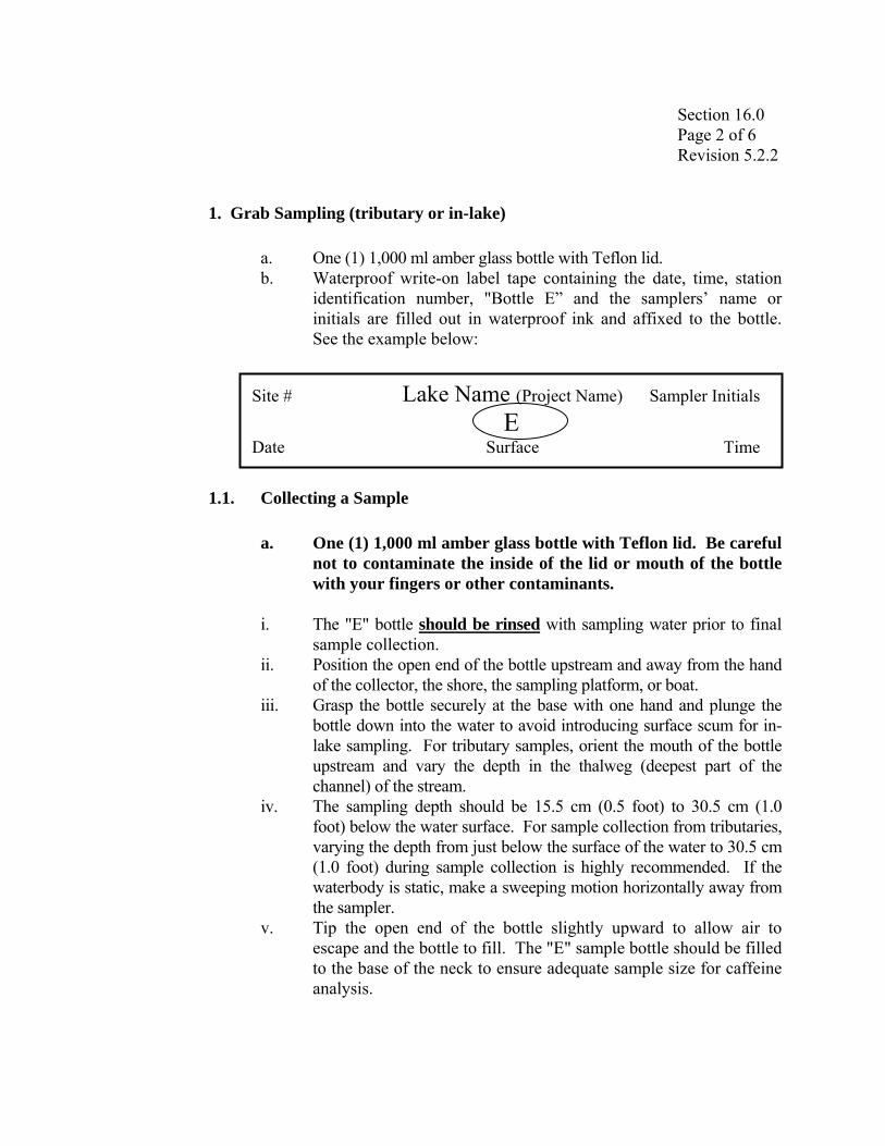
Section 16.0 Page 2 of 6 Revision 5.2.2
1. Grab Sampling (tributary or in-lake)
a. One (1) 1,000 ml amber glass bottle with Teflon lid. b. Waterproof write-on label tape containing the date, time, station
identification number, "Bottle E” and the samplers’ name or initials are filled out in waterproof ink and affixed to the bottle. See the example below:
1.1. Collecting a Sample
a. One (1) 1,000 ml amber glass bottle with Teflon lid. Be careful not to contaminate the inside of the lid or mouth of the bottle with your fingers or other contaminants.
i. The "E" bottle should be rinsed with sampling water prior to final
sample collection. ii. Position the open end of the bottle upstream and away from the hand
of the collector, the shore, the sampling platform, or boat. iii. Grasp the bottle securely at the base with one hand and plunge the
bottle down into the water to avoid introducing surface scum for in-lake sampling. For tributary samples, orient the mouth of the bottle upstream and vary the depth in the thalweg (deepest part of the channel) of the stream.
iv. The sampling depth should be 15.5 cm (0.5 foot) to 30.5 cm (1.0 foot) below the water surface. For sample collection from tributaries, varying the depth from just below the surface of the water to 30.5 cm (1.0 foot) during sample collection is highly recommended. If the waterbody is static, make a sweeping motion horizontally away from the sampler.
v. Tip the open end of the bottle slightly upward to allow air to escape and the bottle to fill. The "E" sample bottle should be filled to the base of the neck to ensure adequate sample size for caffeine analysis.
Site # Lake Name (Project Name) Sampler Initials
E Date Surface Time
Section 16.0 Page 3 of 6 Revision 5.2.2
vi. After filling, screw on the Teflon-lined cap on the sample bottle
and place sample bottle in cooler with ice. vii. No preservative is placed in this bottle. Caffeine samples only
require cooling to 4o C for preservation. All samples must be kept at 4º C prior to and during shipping samples to the laboratory.
viii. Fill out SD DENR Water Quality Data Sheets to ship with the samples (Appendix A).
2. Composite Sampling (tributary and in-lake)
Composite samples are samples that contain water from more than one location or site (in-lake composite samples) or more than one location along a transect across a tributary stream or river. The sample collection is the only thing that differs from the grab sample. All other aspects of sample handling can be found in the Grab Sample section.
2.1. Collecting the Sample
Tributary
a. Select a representative transect across a stream or river and determine the number and positions of sub-samples that will be collected across the transect (minimum of three).
b. Determine the sample volume needed from each sub-sample as per the in-lake caffeine composite sampling section.
c. In wadable streams, collect separate samples in separate amber glass bottles from predetermined locations along a transect, following the methods outlined in the grab sampling section.
d. Return filled sub-sample jars to the shore and pour the predetermined sub-sample volume from one sub-sample jar into a pre-rinsed, glass, graduated cylinder.
e. Pour the water from the graduated cylinder into a pre-rinsed composite sample bottle.
f. Repeat procedures “d.” and “e.” on the remaining sub-sample jars.

Section 16.0 Page 4 of 6 Revision 5.2.2
g. For larger (non-wadable) streams, collect sub-samples from a
boat following the grab sampling methods at each sub-sampling site.
h. After filling the composite sample bottle, screw on the Teflon-lined cap on the sample bottle and place sample bottle in cooler with ice.
In-lake
a. The sampling plan will determine which samples are to be
composite samples. b. Pre-rinse a glass, graduated cylinder twice with sample water. c. Collect a sample in a rinsed Van Dorn (Alpha Bottle)
Sampler (In-lake Sampling Section) or other sampling container.
d. Rinse the sample container with a portion of the water collected.
e. Calculate the amount water needed from each sub-sample. Divide the size of your container (milliliters), by the number of sampling sites to be composited.
Example: Compositing five sites and placing them in the “E”
bottle (1,000 ml).
1000 ml/ 5 = 200 ml
f. Pour the previously calculated amount from one sub-sample into the graduated cylinder.
g. Pour the water from the graduated cylinder into a pre-rinsed sample bottle.
h. Repeat procedures “f.” and “g.” on the remaining sub-sample sites.
i. Preserve the sample bottles following the procedures below.

Section 16.0 Page 5 of 6 Revision 5.2.2
D. Shipping the Sample
General Samples
1. Completely fill out a SD DENR Water Quality Data Sheet (Appendix A) for each site/station/sample in the cooler.
2. All sample containers (bottles) are placed in a large plastic bag. Seal/tie the plastic bag and place the plastic bag with the samples into a shipping cooler.
3. Ice will be placed in two heavy plastic bags, which is then placed in the cooler with the samples.
4. Make sure that all SD DENR Water Quality Data Sheets (Appendix A) are filled out completely (one sample sheet for each sampling site in the cooler). These documents are placed inside the cooler between the insulation and cardboard lid.
5. Address and securely seal the coolers with clear packing tape. 6. Coolers are shipped or taken by the sampler to the State Health Laboratory at
the address below or other contracted laboratory where analyses are performed.
South Dakota Public Health Laboratory 615 East Fourth Street Pierre, South Dakota 57501-1700
Chain-of-Custody Samples
1. Completely fill out a SD DENR Water Quality Data Sheet (Appendix A) for each site/station/sample in the cooler. The SD DENR Water Quality Data Sheet also serves the chain-of-custody document which documents/identifies all samples in the cooler.
2. All sample containers (bottles) are placed in a large plastic bag. Sign, date and write the word “SEALED” on a chain-of-custody seal. Seal the plastic bag with a chain-of-custody seal and place a strip of clear packing tape around seal. Place the plastic bag with the samples into a shipping cooler.
Section 16.0 Page 6 of 6 Revision 5.2.2
3. Ice will be placed in two heavy plastic bags, which is then placed in the
cooler with the samples. 4. Make sure that all SD DENR Water Quality Data Sheets (Appendix A) are
filled out completely (one sample sheet for each sampling site in the cooler). 5. Sign and fill in date and time in the Lab Comments section of the SD DENR
Water Quality Data Sheets to complete chain-of-custody. 6. Retain one copy of each of the SD DENR Water Quality Data Sheets (chain-
of-custody record), and send the original copies with the samples. Place all remaining copies of the SD DENR Water Quality Data Sheets inside the cooler between the insulation and cardboard lid.
7. Sign, date and write the word “SEALED” on a chain-of-custody seal. 8. Place the chain-of-custody seal across the lid and on to the box to seal the
shipping cooler and place clear packing tape over the chain-of-custody seal. 9. Securely seal the cooler with clear packing tape. 10. Coolers are shipped or taken by the sampler to the State Health Laboratory at
the address below or other contracted laboratory where analyses are performed.
South Dakota Public Health Laboratory 615 East Fourth Street Pierre, South Dakota 57501-1700
E. QA/QC Samples Quality assurance/quality control procedures are presented in Section 8.0.

Section 17.0 Page 1 of 4 Revision 5.2.2
17.0. METAL SAMPLING
South Dakota Water Resources Assistance Program (SD WRAP) will provide the preservative for metal sampling. Most metals are preserved with nitric acid (HNO3); however, refer to Table 10.0.1 for specific preservative requirements. For some sampling situations, samples will be collected, cooled to 4 ºC and shipped on ice to the contracting laboratory within 24 hours and preserved at the laboratory.
A. Sample Collection
1. Tributary sample collection techniques (see section 12.0). 2. In-lake sample collection techniques (see section 14.0).
B. Sampling Procedures
1. Tributary sampling Secure one (1) 1000 ml High-Density Polyethylene (HDPE) bottle.
a. Label sample bottle using waterproof pen with project name, site
number, metals, samplers’ initials, date, surface or bottom and time.
b. Pre-rinse sample bottle with sample water prior to sample collection. c. Position the open end of the sample bottle towards the current flow
and away from the hand of the collector. a. Grasp bottle securely at the base and plunge the entire bottle below
the water surface. b. Sampling depth should be 15.5 cm (0.5 foot) to 30.5 cm (1.0 foot)
below the water surface. c. Tip the sample bottle slightly upward to allow air to escape and the
bottle to fill. d. Fill metals bottle to volume similar to the “A” and “B” bottles in
Figure 14.0.2.
Site # Tributary Name (Project Name) Sampler Initials Metals
Date Surface/Bottom Time

Section 17.0 Page 2 of 4 Revision 5.2.2
e. Preserve the sample by adding 1 ml of concentrated HNO3 (Nitric
Acid) to bring the sample below a pH of 2 standard units. f. Completely fill out a SD WRAP Water Quality Data Sheet and a
Chain of Custody Sheet for each sampling site. g. If no preservative was provided, package the samples in a cooler on
ice (4 ºC) and ship to the contracting laboratory within 24 hours to be preserved.
h. Ship samples in sample cooler on ice to the contracting laboratory as described in Section 17.0 (C) below.
2. Lake sampling
Secure one (1) 1000 ml High-Density Polyethylene (HDPE) bottle. a. Label sample bottle with project name, site number, samplers’ initials,
metals, date, surface or bottom and time. See below:
b. Pre-rinse sample bottle with sample water prior to sample collection. c. Collect water sample following collection procedures outlined in Section
14.0 (C) (In-lake Water Sampling Method (Van Dorn-type sampler)). d. The metals bottle should be filled directly from water collected with the
Van Dorn sampler by opening and closing the petcock valve on the Van Dorn-type sampler.
e. Fill metals bottle to volume similar to the “A” and “B” bottles in Figure 14.0.2.
f. Preserve the sample by adding 1 ml of concentrated HNO3 (Nitric Acid) to bring the sample pH below 2 standard units (su).
g. Completely fill out a SD WRAP Water Quality Data Sheet and a Chain of Custody Sheet for each sampling site.
h. If no preservative was provided, package the samples in a cooler on ice (4 ºC) and ship to the contracting laboratory within 24 hours to be preserved.
i. Ship samples to the contracting laboratory following Section 17.0 (C).
Site # Lake Name (Project Name) Sampler Initials Metals
Date Surface/Bottom Time

Section 17.0 Page 3 of 4 Revision 5.2.2
C. Shipping the Sample
General Samples
1. Completely fill out a SD DENR Water Quality Data Sheet (Appendix A) for each site/station/sample in the cooler.
2. All sample containers (bottles) are placed in a large plastic bag. Seal/tie the plastic bag and place the plastic bag with the samples into a shipping cooler.
3. Ice will be placed in two heavy plastic bags, which is then placed in the cooler with the samples.
4. Make sure that all SD DENR Water Quality Data Sheets (Appendix A) are filled out completely (one sample sheet for each sampling site in the cooler). These documents are placed inside the cooler between the insulation and cardboard lid.
5. Securely seal the cooler with clear packing tape. 6. Coolers are shipped or taken by the sampler to the State Health Laboratory at
the address below or other contracted laboratory where analyses are performed.
South Dakota Public Health Laboratory 615 East Fourth Street Pierre, South Dakota 57501-1700
Chain-of-Custody Samples
1. Completely fill out a SD DENR Water Quality Data Sheet (Appendix A) for each site/station/sample in the cooler. The SD DENR Water Quality Data Sheet also serves the chain-of-custody document which documents/identifies all samples in the cooler.
2. All sample containers (bottles) are placed in a large plastic bag. Sign, date and write the word “SEALED” on a chain-of-custody seal. Seal the plastic bag with a chain-of-custody seal and place a strip of clear packing tape around seal. Place the plastic bag with the samples into a shipping cooler.

Section 17.0 Page 4 of 4 Revision 5.2.2
3. Ice will be placed in two heavy plastic bags, which is then placed in the cooler
with the samples. 4. Make sure that all SD DENR Water Quality Data Sheets (Appendix A) are filled
out completely (one sample sheet for each sampling site in the cooler). 5. Sign and fill in date and time in the Lab Comments section of the SD DENR
Water Quality Data Sheets to complete chain-of-custody. 6. Retain one copy of each of the SD DENR Water Quality Data Sheets (chain-of-
custody record), and send the original copies with the samples. Place all remaining copies of the SD DENR Water Quality Data Sheets inside the cooler between the insulation and cardboard lid.
7. Sign, date and write the word “SEALED” on a chain-of-custody seal. 8. Place the chain-of-custody seal across the lid and on to the box to seal the
shipping cooler and place clear packing tape over the chain-of-custody seal. 9. Securely seal the cooler with clear packing tape. 10. Coolers are shipped or taken by the sampler to the State Health Laboratory at
the address below or other contracted laboratory where analyses are performed.
South Dakota Public Health Laboratory 615 East Fourth Street Pierre, South Dakota 57501-1700
D. QA/QC Samples
Quality assurance/quality control procedures are presented in Section 8.0.

Section 18.0 Page 1 of 8 Revision 5.2.2
18.0. ELUTRIATE SAMPLING (Lake Sediment Sampling)
A. Purpose
This method is generally aimed to test sediment for contaminants for future dredge projects and eventual land application and to produce information about contaminants that may affects the benthic community. This method is used as a screening process by the field technician or may be designated in the work plan. The choice of specific sampling sites is based primarily on field reconnaissance, known flow patterns through the lake, locations of tributary inputs, and any other known point sources which may affect the outcome and distribution of the sediment contaminants. This sampling method will be used to collect sediment samples used as general screening for specific pollutants identified in the Project Implementation Plan (PIP).
B. Materials
Sampling Equipment
1. Boat or Ice Auger and Chipping Bar.
a. Life jackets (use in boat or on ice). b. Other required safety equipment.
2. Sediment Samplers
a. Corer (Benthos Gravity, Alpine Gravity, Phleger, Multiple). b. Grab (Franklin Anderson, Dietz-LaFond, Peterson, Shipek,
Ponar). c. Dredge (Birge-Ekman).
3. Five one-gallon glass jars (with Teflon-lined lids) per sampling site. 4. Shipping cooler(s). 5. One (1) clean 18.9 liter (5 gallon) bucket for each grab sampling site.
Two (2) 18.9 liter (5 gallon) buckets will be needed if composite samples are required.
6. SD DENR Contaminates Sample Data Sheet and Chain of Custody Labels and sheets (Appendix A).
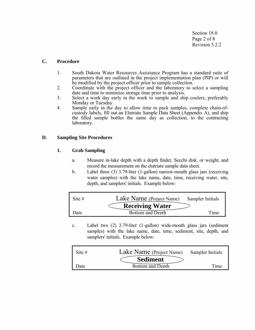
Section 18.0 Page 2 of 8 Revision 5.2.2
C. Procedure
1. South Dakota Water Resources Assistance Program has a standard suite of parameters that are outlined in the project implementation plan (PIP) or will be modified by the project officer prior to sample collection.
2. Coordinate with the project officer and the laboratory to select a sampling date and time to minimize storage time prior to analysis.
3. Select a work day early in the week to sample and ship coolers, preferably Monday or Tuesday.
4. Sample early in the day to allow time to pack samples, complete chain-of-custody labels, fill out an Elutriate Sample Data Sheet (Appendix A), and ship the filled sample bottles the same day as collection, to the contracting laboratory.
D. Sampling Site Procedures
1. Grab Sampling
a. Measure in-lake depth with a depth finder, Secchi disk, or weight, and record the measurement on the elutriate sample data sheet.
b. Label three (3) 3.79-liter (1-gallon) narrow-mouth glass jars (receiving water samples) with the lake name, date, time, receiving water, site, depth, and samplers' initials. Example below:
c. Label two (2) 3.79-liter (1-gallon) wide-mouth glass jars (sediment
samples) with the lake name, date, time, sediment, site, depth, and samplers' initials. Example below:
Site # Lake Name (Project Name) Sampler Initials Sediment
Date Bottom and Depth Time
Site # Lake Name (Project Name) Sampler Initials Receiving Water
Date Bottom and Depth Time

Section 18.0 Page 3 of 8 Revision 5.2.2
d. Being careful not to disturb the lake bottom, obtain samples of water
from near the bottom of the lake using a pre-rinsed Van Dorn, Kemmerer bottle, or other non-contaminating sampler.
e. Completely fill three (3) 3.79-liter (1-gallon) narrow-mouth glass jars with water obtained from step ‘d’ above (receiving water). Securely cap the jars with Teflon-lined lids.
f. Place receiving water sample bottles into a large heavy plastic bag and seal it with a chain-of-custody label and place sealed plastic bag into the sampling cooler.
g. After receiving water samples are completed, collect sediment samples with a Ponar or other appropriate sediment sampler. Place the sediment collected from sampler grabs into a pre-cleaned 18.9-liter (5-gallon) bucket.
h. Mix the sediment in the pre-cleaned bucket with latex gloves to homogenize the sample.
i. Completely fill two 1-gallon wide-mouth glass jars with sediment per sampling site. Make sure that container is completely filled with sediment and that air bubbles are not trapped in the container. Carefully rinse the glass jar threads and the cap with sample water to clean the threads for a better seal. Securely cap with Teflon-lined lid.
j. Place sediment sample bottles into a separate large heavy plastic bag and seal it with a chain-of-custody label and secure it with clear packing tape; place sealed plastic bag into the sampling cooler.
2. Composite Sampling
Composite sediment sampling is similar to grab sampling except separate receiving water and sediment samples are collected throughout the lake and composited.
a. Composite sampling sites will be defined in the Project Implementation
Plan (PIP) or will be chosen by the project officer. b. Two (2) pre-rinsed buckets will be needed for compositing
(homogenizing) receiving water and sediment samples. One (1) 18.9-liter (5-gallon) bucket will be used to composite (homogenize) three 11.4 liters (3-gallons) of receiving water and one (1) 18.9-liter (5-gallon) bucket to composite (homogenize) 7.6 liters (2-gallons) of sediment.
c. Determine the appropriate amount of receiving water and sediment to collect from each sub-sampling site. See procedure below:

Section 18.0 Page 4 of 8 Revision 5.2.2
i. To calculate the amount receiving water and sediment needed from each sub-sample. Divide the minimum amount of sample needed in liters, by the number of sampling sites to be composited. See below:
Receiving Water Example When compositing 3 sites for receiving water (11.4 liters (3-gallons) required).
11.4 liters (3-gallons) / 3 sites = 3.8 liters (1-gallon)
Pour the previously calculated amount of receiving water into the pre-rinsed 18.9-liter (5-gallon) bucket. Collect this volume at all remaining sub-sampling sites.
Sediment Example
When compositing 3 sites for sediment (7.6 liters (2-gallons) required).
7.6 liters (2-gallons) / 3 sites = 2.5 liters (0.67-gallon)
Pour the previously calculated amount of receiving water into the pre-rinsed 18.9-liter (5-gallon) bucket. Collect this volume at all remaining sub-sampling sites.
d. Label three (3) 3.79-liter (1-gallon) narrow-mouth glass jars (receiving water samples) with the lake name, date, time, receiving water, site, depth, composite and samplers' initials. Example below:
e. Label two (2) 3.79-liter (1-gallon) wide-mouth glass jars (sediment samples) with the lake name, date, time, sediment, site, depth, composite and samplers' initials. Example below:
Site # Lake Name (Project Name) Sampler Initials Receiving Water
Date Bottom and Depth COMPOSITE Time

Section 18.0 Page 5 of 8 Revision 5.2.2
f. At each sub-sampling site, measure in-lake depth with a depth finder, Secchi disk, or weight, and record each depth measurement on the elutriate sample data sheet under composite sample depth.
g. At the first sub-sampling site, being careful not to disturb the lake bottom, obtain the previously calculated volume of water from near the bottom of the lake using a pre-rinsed Van Dorn, Kemmerer bottle, or other non-contaminating sampler and pour it into a pre-rinsed 18.9 liter (5-gallon) bucket.
h. After collecting the receiving water sample at the sub-sampling site, collect a sediment sub-sample with a Ponar or other appropriate sediment sampler. Place the sediment collected from sampler grabs into a pre-cleaned 18.9 liter (5-gallon) bucket.
i. Repeat procedure ‘g’ and ‘h’ at the remaining sub-sampling sites. j. Stir or swirl receiving water to homogenize the sample. k. After all composite samples (receiving water and sediment) have been
collected, completely fill three (3) 3.79-liter (1-gallon) narrow-mouth glass jars with water from the receiving water composite sample (18.9 liter (5-gallon) bucket). Securely cap the jars with Teflon-lined lids.
l. Place receiving water sample bottles into a large heavy plastic bag and seal it with a chain-of-custody label and place sealed plastic bag into the sampling cooler.
m. Mix the sediment composite sample in the 18.9 liter (5-gallon) bucket with latex gloves to homogenize the sample.
n. Completely fill two (2) 1-gallon wide-mouth glass jars with sediment per sampling site. Make sure that container is completely filled with sediment and that air bubbles are not trapped in the container. Carefully rinse the glass jar threads and the cap with sample water to clean the threads for a better seal. Securely cap with Teflon-lined lid.
Site # Lake Name (Project Name) Sampler Initials Sediment
Date Bottom and Depth COMPOSITE Time
Section 18.0 Page 6 of 8 Revision 5.2.2
E. Shipping the Sample
General Samples
1. Completely fill out an SD DENR Contaminates Sample Data Sheet(s) (write in “Elutriate Sample” in the Field Comments section of the data sheet) are filled out completely (one sample sheet for each sampling site in the cooler).
2. All sample containers (sample bottles) are placed in large plastic bags. Seal/tie the plastic bags and place with the samples in the shipping cooler.
3. Ice will be placed in two heavy plastic bags, which is then placed in the cooler with the samples.
4. Place SD DENR Contaminates Sample Data Sheet(s) into a large ziploc freezer bag.
5. Place the freezer bag with the completed SD DENR Contaminates Sample Data Sheet into the cooler, address and securely seal the cooler with clear packing tape.
6. Care should be taken when handling/lifting the cooler(s) due to excess weight.
7. Coolers are shipped or taken by the sampler to the State Health Laboratory at the address below or other contracted laboratory where analyses are performed.
South Dakota Public Health Laboratory 615 East Fourth Street Pierre, South Dakota 57501-1700
8. SHIP OR TRANSPORT THE SAMPLES TO THE LAB THE SAME DAY AS COLLECTION, IF AT ALL POSSIBLE.
Chain-of-Custody Samples
1. Completely fill out a SD DENR Contaminates Sample Data Sheet(s) (Appendix A) for each site/station/sample in the cooler. The SD DENR Contaminates Sample Data Sheet also serves the chain-of-custody document which documents/identifies all samples in the cooler.
2. All sample containers (sample bottles) are placed in large plastic bags. Sign, date and write the word “SEALED” on a chain-of-custody seal(s). Seal the plastic bag with a chain-of-custody seal and place a strip of clear packing tape around seal. Place the plastic bag with the samples into a shipping cooler.

Section 18.0 Page 7 of 8 Revision 5.2.2
3. Ice will be placed in two heavy plastic bags, which is then placed in the cooler with the samples.
4. Make sure that all SD DENR Contaminates Sample Data Sheet(s) (Appendix A) are filled out completely (one sample sheet for each sampling site in the cooler) and write in “Elutriate Sample” in the Field Comments section of the data sheet.
5. Sign and fill in date and time in the Lab Comments section of the SD DENR Contaminates Sample Data Sheet(s) to complete chain-of-custody.
6. Retain one copy of the chain-of-custody record, and send the original copy with the samples. .Place all remaining copies of the SD DENR Contaminates Sample Data Sheet(s) into a large ziploc freezer bag.
7. Place the freezer bag with the completed SD DENR Contaminates Sample Data Sheet into the cooler.
8. Sign, date and write the word “SEALED” on two chain-of-custody seals 9. Place the chain-of-custody seals across the lid and on to the box to seal the
shipping cooler and place clear packing tape over chain-of-custody seal. 10. Address and securely seal the cooler with clear packing tape. 11. Care should be taken when handling/lifting the cooler(s) due to excess
weight. 12. Coolers are shipped or taken by the sampler to the State Health Laboratory at
the address below or other contracted laboratory where analyses are performed.
South Dakota Public Health Laboratory 615 East Fourth Street Pierre, South Dakota 57501-1700
13. SHIP OR TRANSPORT THE SAMPLES TO THE LAB THE SAME
DAY AS COLLECTION, IF AT ALL POSSIBLE.
F. Quality Control (Field)
1. Provide representative samples for analysis. 2. Rinse all containers properly prior to use. 3. Initiate appropriate storage procedures immediately after collection. 4. Properly label and record dates and locations of sample collections, as well as
other pertinent information, on the elutriate sample data sheet. 5. Complete the chain-of-custody record and retain one copy for the project files.

Section 18.0 Page 8 of 8 Revision 5.2.2
G. Quality Control (Lab)
The laboratory chosen for analysis of samples should provide the following quality control functions:
1. Use scientifically acceptable techniques for analysis. 2. Complete analyses within prescribed parameter-specific holding times limits. 3. Perform replicate analyses on approximately 5 to 10 percent of samples
processed. 4. Use internal laboratory standards to check performance of analytical methods.
Section 19.0 Page 1 of 3 Revision 5.2.2
19.0 DISCRETE GRAB SAMPLES FOR UPSTREAM AND DOWNSTREAM
SAMPLING
A. Site Location
Sampling site locations are specified in the Project Implementation Plan (PIP) and/or by the project officer. Downstream samples are always collected first to lessen potential contamination and impact.
1. Locate the downstream site between one hundred yards and one mile downstream from the potential pollution source.
a. Do not sample in any ponded or pooled areas because of backwater
impacts. If the closest access point is on private land, be sure to have permission before sampling. If at all possible, sample in public right-of-ways which require no permission.
b. If the source being sampled has no direct discharge, make sure you have sampled downstream of the suspected impact area.
c. Be sure there are no unknown pollution sources in the area you are trying to sample; if there are, document on the water quality data sheet.
2. Locate the upstream site between one hundred yards and one mile upstream from the potential pollution source.
a. Do not sample in any ponded or pooled areas because of backwater impacts. If the closest access point is on private land, be sure to have permission before sampling. If at all possible, sample in public right-of-ways which require no permission.
b. Ensure upstream sampling site is far enough upstream of the potential impacted area as to not influence the upstream sample.
c. If there are potential impacts (point sources or other pollution concerns) above the upstream sampling site, document this on the water quality data sheet.
3. At times the water in the tributary will travel for long distances before mixing with the contaminated water. If distinct zones of water are observed, move the sampling site further downstream to where the waters have mixed.

Section 19.0 Page 2 of 3 Revision 5.2.2
B. Sample Collection
1. Follow the equipment calibration procedures presented in Section 6.0 of this manual.
2. Follow the tributary sampling procedures presented in Section 12.0 of this manual.
C. Shipping Samples
General Samples
1. Completely fill out an SD DENR Water Quality Data Sheets are filled out completely (one sample sheet for each sampling site in the cooler).
2. All sample containers (bottles) are placed in a large plastic bag. Seal/tie the plastic bag and place the plastic bag with the samples into a shipping cooler.
3. Ice will be placed in two heavy plastic bags, which is then placed in the cooler with the samples.
4. Make sure that all SD DENR Water Quality Data Sheets (Appendix A) are filled out completely (one sample sheet for each sampling site in the cooler). These documents are placed inside the cooler between the insulation and cardboard lid.
5. Securely seal the cooler with clear packing tape. 6. Coolers are shipped or taken by the sampler to the State Health Laboratory at
the address below or other contracted laboratory where analyses are performed.
South Dakota Public Health Laboratory 615 East Fourth Street Pierre, South Dakota 57501-1700
Chain-of-Custody Samples
1. Completely fill out a SD DENR Water Quality Data Sheet(s) (Appendix A) for each site/station/sample in the cooler. The SD DENR Water Quality Data Sheets also serves the chain-of-custody document which documents/identifies all samples in the cooler.

Section 19.0 Page 3 of 3 Revision 5.2.2
2. All sample containers (sample bottles) are placed in large plastic bags. Sign, date and write the word “SEALED” on a chain-of-custody seal(s). Seal the plastic bag with a chain-of-custody seal and place a strip of clear packing tape around seal. Place the plastic bag with the samples into a shipping cooler.
3. Ice will be placed in two heavy plastic bags, which is then placed in the cooler with the samples.
4. Make sure that all SD DENR Water Quality Data Sheet(s) (Appendix A) are filled out completely (one sample sheet for each sampling site in the cooler) filled out.
5. Sign and fill in date and time in the Lab Comments section of the SD DENR Water Quality Data Sheet(s) to complete chain-of-custody.
6. Retain one copy of each of the SD DENR Water Quality Data Sheets (chain-of-custody record), and send the original copies with the samples. Place all remaining copies of the SD DENR Water Quality Data Sheets inside the cooler between the insulation and cardboard lid.
7. Sign, date and write the word “SEALED” on two chain-of-custody seals 8. Place the chain-of-custody seals across the lid and on to the box to seal the
shipping cooler and place clear packing tape over chain-of-custody seal. 9. Address and securely seal the cooler with clear packing tape. 10. Coolers are shipped or taken by the sampler to the State Health Laboratory at
the address below or other contracted laboratory where analyses are performed. South Dakota Public Health Laboratory 615 East Fourth Street Pierre, South Dakota 57501-1700

Section 20.0 Page 1 of 7 Revision 5.2.2
20.0 PESTICIDE SAMPLING
A. Purpose
This method is used to collect water samples to screen for specific pollutants identified in the Project Implementation Plan (PIP), identified in elutriate sampling and/or specified by the project officer. This method is also generally aimed to produce information on pesticide contamination that may affect the benthic community as a whole.
B. Materials
Basic Sampling Equipment 1. Boat or Ice Auger and Chipping Bar. 2. Van Dorn (Alpha Bottle), Kemmerer bottle, Integrated Sediment Sampler or
other non-contaminating sampler. 3. 1-gallon of pre-mixed 10% Acetone solution. 4. Squirt bottle. 5. Plastic tray. 6. Empty plastic 1-gallon jug (for waste Acetone solution). 7. 2-gallons of de-ionized water for rinsing sampler. 8. Amber glass jars / Teflon-lined lids. 9. Shipping coolers. 10. Logbook. 11. Chain of custody labels and records.
C. Procedure
1. Determine specific tests and analyses to be completed. Specific parameters are outlined in the Project Implementation Plan (PIP) or will be determined by the project officer. The selection of chemical parameters to be analyzed should be based on major point sources and contaminants of concern in the project area. Because of site-specific variability, no mandatory or minimum list of analyses is recommended. Specific pollutants to be analyzed for should be based on the potential of pesticides occurring in the watershed in addition to people expressing concern over other pollutants.
2. Contact the laboratory for the specific type(s) of sample containers, volume(s) and preservative needed for pesticides to be sampled or consult section 10.0 of this manual.
3. The number of pesticide samples required should be outlined in the PIP. If specific locations are not identified, the project officer will determine sampling sites.
Section 20.0 Page 2 of 7 Revision 5.2.2
4. Coordinate with the project officer and the laboratory to select the sampling
date and time to minimize storage time prior to analysis. 5. Select a work day early in the week to sample and ship coolers, preferably
Monday or Tuesday. 6. Sample early in the day to allow time to pack samples, complete chain-of-
custody labels, fill out State Health Laboratory Data Sheets (Appendix A), and ship the filled sample bottles the same day as collection, to the contracting laboratory.
7. Always enter all sampling information in the project logbook Section 5.0.
D. Sampling Procedures
1. Tributary Procedures
Secure one (1) 1000-ml amber glass bottle with a Teflon-lined lid.
a. Label sample bottle using waterproof pen with project name, site number, pesticides, samplers’ initials, date, surface or bottom and time.
b. Pre-rinse sample bottle with de-ionized water prior to sample collection.
c. Position the open end of the sample bottle towards the current flow and away from the hand of the collector.
d. Grasp bottle securely at the base and plunge the entire bottle below the water surface.
e. Sampling depth should be 15.5 cm (0.5 foot) to 30.5 cm (1.0 foot) below the water surface.
f. Tip the sample bottle slightly upward to allow air to escape and the bottle to fill.
g. Fill pesticides bottle to the bottom of the neck. h. Preserve the sample depending on parameter, please refer to Table
10.0.2. i. Completely fill out an SD DENR Contaminates Sample Data Sheet (write
in “Pesticide Sample” in the Field Comments section of the data sheet) and chain-of-custody record for each sampling site.
Site # Tributary Name (Project Name) Sampler InitialsPesticides
Date Surface/Bottom Time
Section 20.0 Page 3 of 7 Revision 5.2.2
j. Completely record all sample collection information in the project
logbook. k. If no preservative was provided package the samples in a cooler on
ice (4 ºC) and ship to the contracting laboratory within 24 hours to be preserved.
l. Ship samples in sample cooler on ice to the contracting laboratory as described in Section 20.0 (E) below.
2. In-lake Procedures
a. Grab Sampling (without a sampling device)
This sampling technique is only used for surface samples. Secure one (1) 1000-ml amber glass bottle with Teflon lined lid.
i. Label sample bottle using waterproof pen with project name, site number, pesticides, samplers’ initials, date, surface or bottom and time.
ii. Pre-rinse sample bottle with de-ionized water prior to sample collection.
iii. Position the open end of the sample bottle away from the shore, dock or boat and away from the hand of the collector.
iv. Grasp bottle securely at the base and plunge the entire bottle below the water surface.
v. Sampling depth should be 15.5 cm (0.5 foot) to 30.5 cm (1.0 foot) below the water surface.
vi. Tip the sample bottle slightly upward to allow air to escape and the bottle to fill.
vii. Fill pesticides bottle to the bottom of the neck. viii. Preserve the sample depending on parameter, please refer to
Table 10.0.2. ix. Completely fill out an SD DENR Contaminates Sample Data
Sheet (write in “Pesticide Sample” in the Field Comments section of the data sheet) and chain-of-custody record for each sampling site.
Site # Tributary Name (Project Name) Sampler InitialsPesticides
Date Surface Time

Section 20.0 Page 4 of 7 Revision 5.2.2
x. Completely record all sample collection information in the project logbook.
xi. If no preservative was provided, package the samples in a cooler on ice (4 ºC) and ship to the contracting laboratory within 24 hours to be preserved.
xii. Ship samples in a sample cooler on ice to the contracting laboratory as in Section 20.0 (E) below.
b. Grab Sampling (with a sampling device)
i. Label sample bottle with project name, site number, samplers’ initials, metals, date, surface or bottom and time. See below:
ii. Pre-rinse sample bottle with de-ionized water prior to sample collection.
iii. Collect water sample using a decontaminated Van Dorn-type sampler or other in-lake sampling. Decontaminate the in-lake sampler using the following procedure.
aa. Place sampler into an empty plastic tray and stand on
end. bb. Using a squirt bottle, completely rinse the sample
collection device both inside and out with 10% Acetone solution.
cc. Holding the outside of the container, suspend sampler above the Acetone solution in bottom of the plastic tray and rinse sampler three times (3X) with de-ionized water.
iv. The pesticides bottle(s) should be filled directly from water collected with the sampler. Drain the Van Dorn-type sampler by opening and closing the petcock valve on the Van Dorn sampler.
v. Fill pesticides bottle(s) to the bottom of the neck. vi. Preserve the sample depending on parameter, please refer to
Table 10.0.2.
Site # Lake Name (Project Name) Sampler InitialsPesticides
Date Surface/Bottom Time

Section 20.0 Page 5 of 7 Revision 5.2.2
vii. Completely fill out an SD DENR Contaminates Sample Data
Sheet (write in “Pesticide Sample” in the Field Comments section of the data sheet) and chain-of-custody record for each sampling site.
viii. Completely record all sample collection information in the project logbook.
ix. If no preservative was provided package, the samples in cooler on ice (4 ºC) and ship to the contracting laboratory within 24 hours to be preserved.
x. Ship samples to the contracting laboratory as in Section 20.0 (E) below.
3. Shipping Samples
General Samples 1. Completely fill out a SD DENR Contaminates Sample Data Sheet(s)
(Appendix A) for each site/station/sample in the cooler. 2. All sample containers (bottles) are placed in a large plastic bag. Seal/tie
the plastic bag and place the plastic bag with the samples into a shipping cooler.
3. Ice will be placed in two heavy plastic bags, which is then placed in the cooler with the samples.
4. Make sure that all SD DENR Contaminates Sample Data Sheet(s) (Appendix A) are filled out completely (one sample sheet for each sampling site in the cooler). These documents are placed inside the cooler between the insulation and cardboard lid.
5. Securely seal the cooler with clear packing tape. 6. Coolers are shipped or taken by the sampler to the State Health
Laboratory at the address below or other contracted laboratory where analyses are performed. South Dakota Public Health Laboratory 615 East Fourth Street Pierre, South Dakota 57501-1700

Section 20.0 Page 6 of 7 Revision 5.2.2
Chain-of-Custody Samples
1. Completely fill out a SD DENR Contaminates Sample Data Sheet(s) (Appendix A) for each site/station/sample in the cooler. The SD DENR Contaminates Sample Data Sheet(s) also serves the chain-of-custody document which documents/identifies all samples in the cooler.
2. All sample containers (bottles) are placed in a large plastic bag. Sign, date and write the word “SEALED” on a chain-of-custody seal. Seal the plastic bag with a chain-of-custody seal and place a strip of clear packing tape around seal. Place the plastic bag with the samples into a shipping cooler.
3. Ice will be placed in two heavy plastic bags, which is then placed in the cooler with the samples.
4. Make sure that all SD DENR Contaminates Sample Data Sheet(s) (Appendix A) are filled out completely (one sample sheet for each sampling site in the cooler).
5. Sign and fill in date and time in the Lab Comments section of the SD DENR Contaminates Sample Data Sheet(s) to complete chain-of-custody.
6. Retain one copy of each of the SD DENR Contaminates Sample Data Sheet(s) (chain-of-custody record), and send the original copies with the samples. Place all remaining copies of the SD DENR Contaminates Sample Data Sheet(s) inside the cooler between the insulation and cardboard lid.
7. Sign, date and write the word “SEALED” on a chain-of-custody seal. 8. Place the chain-of-custody seal across the lid and on to the box to seal
the shipping cooler and place clear packing tape over the chain-of-custody seal.
9. Securely seal the cooler with clear packing tape. 10. Coolers are shipped or taken by the sampler to the State Health
Laboratory at the address below or other contracted laboratory where analyses are performed.
South Dakota Public Health Laboratory 615 East Fourth Street Pierre, South Dakota 57501-1700

Section 20.0 Page 7 of 7 Revision 5.2.2
4. Quality Control (Field)
1. Provide representative samples for analysis. 2. Provide duplicate samples (approximately 10 percent) to define variation
at a single point. Duplicate samples are collected with two sets of field equipment, or duplicate grab samples are collected. This provides a check of sampling equipment and technique for precision.
3. Provide sufficient amounts of samples to allow detection of targeted pollutants.
4. Initiate appropriate storage procedures immediately after collection. 5. Properly label and record dates and locations of sample collections, as
well as other pertinent information.
5. Quality Control (Lab)
The laboratory chosen for analysis of samples should provide the following quality control functions:
1. Use scientifically acceptable techniques for analysis. 2. Complete analyses immediately (ideally) or within prescribed storage
limits that are parameter-specific. 3. Require replicate sample collection and analysis for approximately 10
percent of samples processed. 4. Analyze references, field blanks, unknown samples, and samples split
with other laboratories for approximately 10 percent of samples processed.
5. Use internal laboratory standards to check performance of analytical methods.

Section 21.0 Page 1 of 1 Revision 5.2.2
21.0 RIBOTYPING SAMPLING
South Dakota Water Resources Assistance Program (SD WRAP) includes ribotyping analysis on various projects. Ribotyping is performed on bacteriological samples cultured for E-coli and identifies the probable source (human or animal) of the E-coli bacteria. Sampling techniques are those for bacteriological (“C” bottle) tributary and in-lake samples described in Section 12.0 (Tributary Sampling Techniques) and Section 14.0 (In-lake Sampling Techniques). Samples must arrive at the contracting laboratory within 24 hours of sample collection.

Section 22.0 Page 1 of 2 Revision 5.2.2
22.0. REFERENCES CITED American Public Health Association, American Waterworks Association, and Water Pollution Control
Foundation. 1995. Standard Methods for the Examination of Water and Wastewater, 16th edition. APHA, Washington, D.C.
Ball, J. 1982. Stream Classification Guidelines for Wisconsin. Wisconsin Dept. Nat. Res. Tech.
Bull., Wisconsin Dept. Nat. Res., Madison, WI. Barbour, M.T., J. Gerritsen, B.D. Snyder, and J.B. Stribling. 1999. Rapid Bioassessment Protocols
for use in Streams and Wadeable Rivers. Office of Water (Wh-553), EPA/444/4-89-001. Washington, D.C.
Flint, R.F. 1955. Pleistocene Geology of Eastern South Dakota. U.S. Geological Survey Professional
Paper 262. 173pp. Hayslip, G.A. 1992. EPA Region 10 In-Stream Biological Monitoring Handbook (Draft). EPA
Region 10, Env. Serv. Div., Seattle, WA. Jessen, R. and R. Lound. 1962. An Evaluation of a Survey Technique for Submerged Aquatic
Plants. Minnesota Dept. of Conservation, Division of Game and Fish, Game Investigational Report No. 6.
King, K.W. 1993. A Bioassessment Method for use in Wyoming Stream and River Water Quality
Monitoring. Wyoming Department of Environmental Quality. 84pp. Minn. DNR. 1993. Manual of Instructions for Lake Survey. Special publication No. 147 pp 3-4 -
3-7. Mulvey, M., L. Caton and R. Hafele. 1992. Oregon Nonpoint Source Monitoring Protocols and
Stream Bioassessment Field Manual - for Macroinvertebrates and Habitat Assessment (Draft). Oregon Dept. Env. Qual. Lab., Biomonitoring Section, Portland, OR.
Nickum, J.G. 1969. Limnological Survey of Lake Tetonkaha and Adjacent Marsh. Unpublished
report. Department of Fish and Wildlife, SDSU, Brookings, South Dakota. Petersen, Jr., R.C. 1992. The RCE: A Riparian, Channel, and Environmental Inventory for Small
Streams in the Agricultural Landscape. Freshwater Biology 27:295-314.
Section 22.0 Page 2 of 2 Revision 5.2.2
Plafkin, J.L., M.T. Barbour, K.D. Porter, S.K. Gross, and R.M. Hughes. 1989. Rapid
Bioassessment Protocols for use in Streams and Rivers. Office of Water (Wh-553), EPA/444/4-89-001. Washington, D.C.
Platts, W.S., W.F. Megahan, and G.W. Minshall. 1983. Methods for Evaluating Stream, Riparian,
and Biotic Conditions. General Tech. Rpt. INT-138. U.S. Dept. Agric., Forest Serv., Ogden, UT.
Rosgen, D. 1996. Applied River Morphology. Wildland Hydrology. Pagosa Springs, CO. Rothrock, E.P. 1943. A Geology of South Dakota I. The Surface. State Geological Survey Bulletin
13. 88 pp. South Dakota State Health Laboratory. 1999. Quality Assurance Program, Pierre, South Dakota. State of Vermont. 1990. Indirect Discharge Rules. Agency of Natural Resources Department of
Environmental Conservation. 244 pp. U.S. Environmental Protection Agency. 1990. Guidance Document for the Development of Quality
Assurance Plans for Indian Tribes. Internal document. 20 pp. Wind River Clean Lakes Program Quality Assurance Plan. 1990. Wind River Environmental Quality
Commission, Shoshone and Northern Arapaho Tribes, Ft. Washakie, Wyoming. 19 pp. U.S. Environmental Protection Agency. 1990. Macroinvertebrate Field and Laboratory Methods
for Evaluating the Biological Integrity of Surface Waters. 600/4-90/030. Office of Research and Development, Washington, D.C. 256 pp.
US EPA. 1991. Volunteer Lake Monitoring: A Methods Manual. EPA 440/4-91-002. Office of
Water. Washington, D.C. Young, R.A., C.A. Onstad, D.D. Bosh, and W.P. Anderson. 1986. AGNPS, Agricultural Nonpoint
Source Pollution Model. USDA-ARS Conservation Research Report 35. Young, R.A., M.A. Oterby and A. Roos. 1982. An Evaluation System to Rate Feedlot Pollution
Potential. USDA-ARS Publication ARM-NC-17.
Appendix A
Water Resources Assistance Program Data Sheets
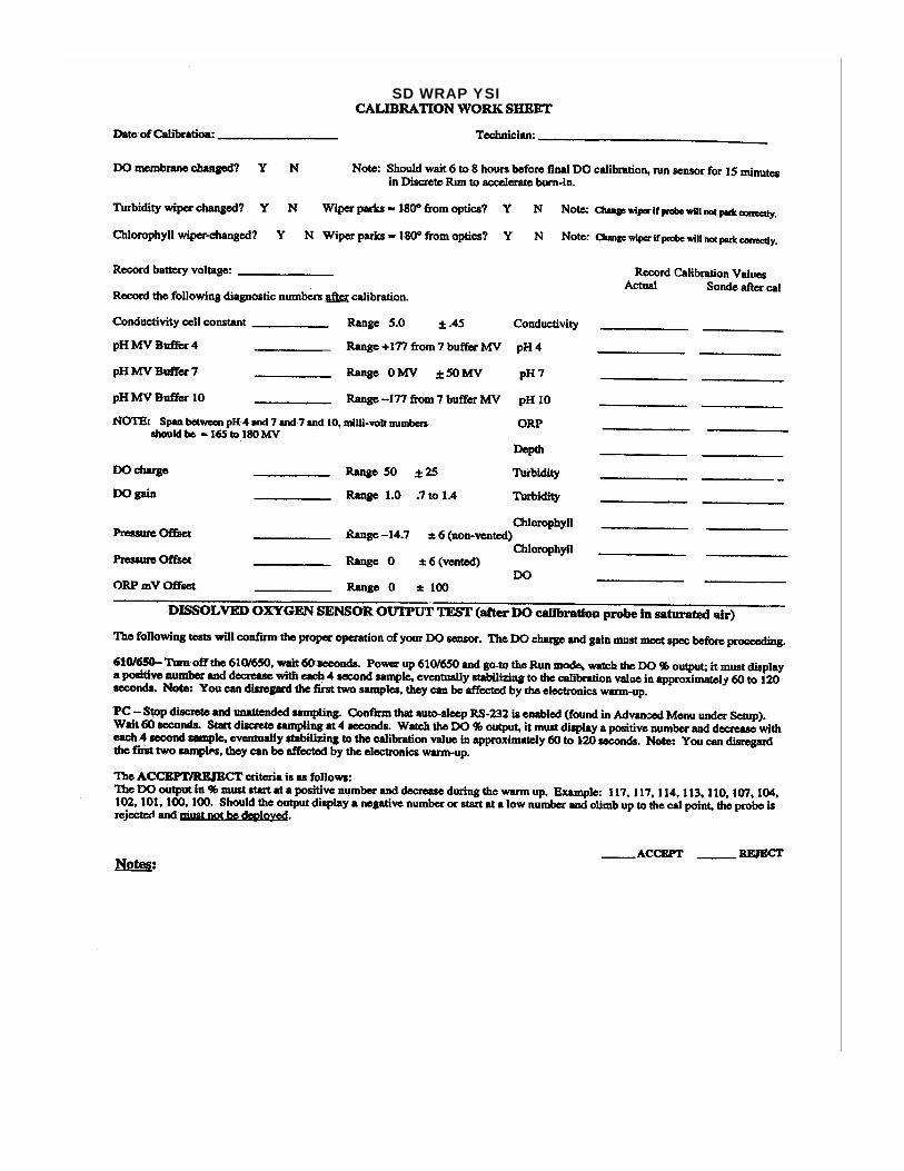
SD WRAP YSI

South Dakota Water Resources Assistance Program In-lake Sampling Field Data Collection Sheet
Lake Name ________________________ Lake ID ___________________ Sampler(s) _________________________ Air Temp. _________________°C Date __________________ Time _________________ MST CST Precip1. N Mi Mo E S Film1: N Mi Mo E S GPS Unit ID _______________________ Wind1: N Mi Mo E S Color ____________ Latitude ___________________________ Odor1: N Mi Mo E S Ice Cover ________ (m)Longitude __________________________ Dead Fish1: N Mi Mo E S 1 = N - None, Mi - Mild, Mo - Moderate, E - Extreme, S - Severe
Site _______________ Site _______________ Site _______________ Tow Length ________(m) Tow Length ________(m) Tow Length ________(m) Depth Temp. DO Depth Temp. DO Depth Temp. DO _____ _____ _____ _____ _____ _____ _____ _____ _____ _____ _____ _____ _____ _____ _____ _____ _____ _____ _____ _____ _____ _____ _____ _____ _____ _____ _____ _____ _____ _____ _____ _____ _____ _____ _____ _____ _____ _____ _____ _____ _____ _____ _____ _____ _____ _____ _____ _____ _____ _____ _____ _____ _____ _____ _____ _____ _____ _____ _____ _____ _____ _____ _____ _____ _____ _____ _____ _____ _____ _____ _____ _____ _____ _____ _____ _____ _____ _____ _____ _____ _____ _____ _____ _____ _____ _____ _____ _____ _____ _____ _____ _____ _____ _____ _____ _____ _____ _____ _____ _____ _____ _____ _____ _____ _____ _____ _____ _____ _____ _____ _____ _____ _____ _____ _____ _____ _____ _____ _____ _____ _____ _____ _____ _____ _____ _____
**** Record depth in meters and temperature in Celsius
Site ______________ Site ______________ Site ______________ Total Depth __________ (m) Total Depth __________ (m) Total Depth ____________ (m) Secchi Depth _____, _____ (m) Secchi Depth _____, _____ (m) Secchi Depth ______, ______ (m) Surface pH ___________ (su) Surface pH ___________ (su) Surface pH ____________ (su) Bottom pH ___________ (su) Bottom pH ____________ (su) Bottom pH ____________ (su) Surface Turbidity _________ (NTU) Surface Turbidity _________ (NTU) Surface Turbidity _________ (NTU) Bottom Turbidity _________ (NTU) Bottom Turbidity _________ (NTU) Bottom Turbidity _________ (NTU) Surface Conduct _________ (µS/cm-1) Surface Conduct _________ (µS/cm-1) Surface Conduct ___________ (µS/cm-1) Bottom Conduct _________ (µS/cm-1) Bottom Conduct _________ (µS/cm-1) Bottom Conduct ___________ (µS/cm-1) Mean Lake Parameters Total Tow Length (for composite zooplankton samples only) _____________ (m) Mean Depth ________________ (m) Mean Secchi Depth ____________ (m) Mean Surface Temperature _______________ °C Mean Bottom Temperature _______________ °C Mean Surface Dissolved Oxygen __________ (mg/L) Mean Bottom Dissolved Oxygen __________ (mg/L) Mean Surface pH ____________ (su) Mean Bottom pH ______________ (su) Mean Surface Turbidity _________ (NTU) Mean Bottom Turbidity ____________ (NTU) Mean Surface Conductivity _________ (µS/cm-1) Mean Bottom Conductivity _________ (µS/cm-1)

SD WRAP Discharge Measurement - Field Data Sheet
Project Site
Sampler Date
Stage Time
Column A Column B Column C Column D Column E
What Tape Reading (in)
Width of Segment (ft)
Depth of Segment (ft)
Velocity at Point (ft/sec)
Total Discharge (CFS)
How Difference of Segment (ft) Depth Gauge Readout Multiply
B x C x D
BANK Cannot be Calculated
1st
2nd
3rd
4th
5th
6th
7th
8th
9th
10th
11th
12th
13th
14th
15th
16th
Total Discharge (CFS) (Sum of Column E)


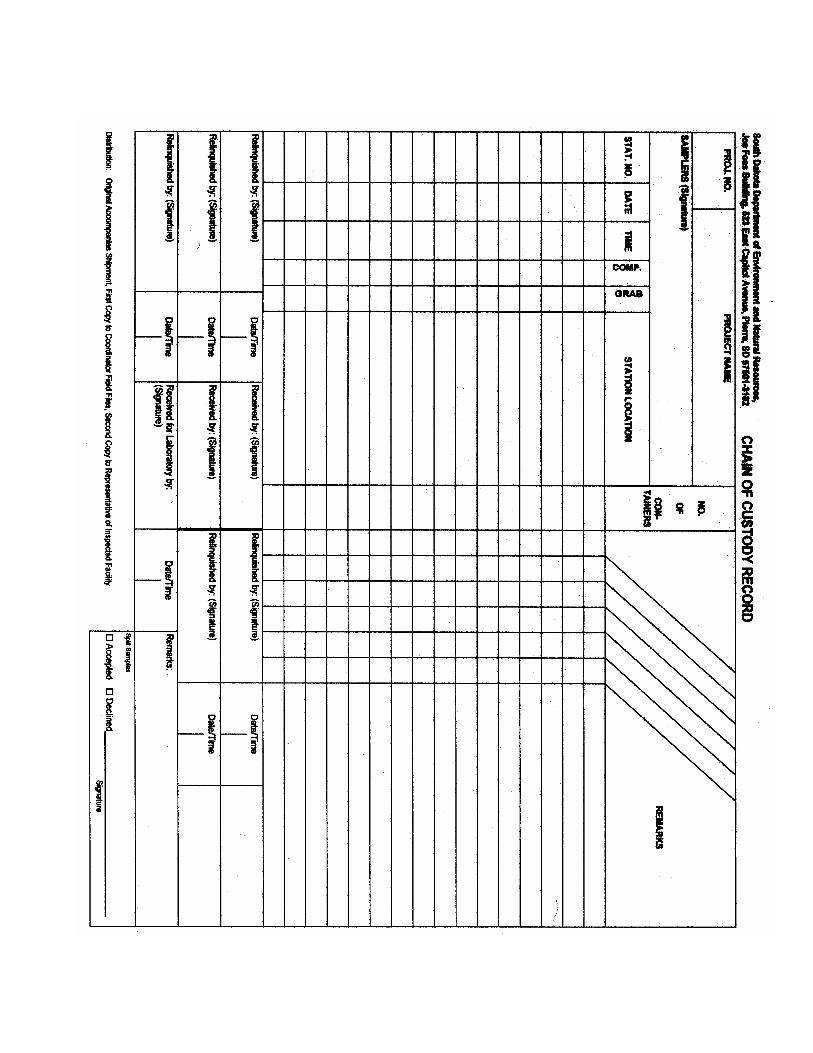


SD DENR Equipment Data Sheet
Date: ___________________________________________ Project: _________________________________________ Coordinator: _____________________________________ Project Officer: ___________________________________
EQUIPMENT SERIAL
NUMBER DATE
ACQUIRED
LOCATION MAINTENANCE
REQUIRED
Signature: __________________________________________, Date: _________________________


75 copies of this document were printed by the Department of Environment and Natural Resources at a cost of $4.20 per copy.


![Operating Procedures 1 G2 - OPERATING PROCEDURES [6 Exam Questions - 6 Groups] G2APhone operating procedures; USB/LSB utilization conventions; procedural.](https://static.fdocuments.us/doc/165x107/56649e4d5503460f94b4351a/operating-procedures-1-g2-operating-procedures-6-exam-questions-6-groups.jpg)