Stacked U-Nets with Multi-Output for Road Extraction

Tao Sun, Zehui Chen, Wenxiang Yang, Yin Wang

Tongji University, Shanghai, China

{suntao, 1652763, twofyw, yinw}@tongji.edu.cn

Abstract

With the recent advances of Convolutional Neural Net-

works (CNN) in computer vision, there have been rapid pro-

gresses in extracting roads and other features from satellite

imagery for mapping and other purposes. In this paper, we

propose a new method for road extraction using stacked U-

Nets with multiple output. A hybrid loss function is used to

address the problem of unbalanced classes of training data.

Post-processing methods, including road map vectorization

and shortest path search with hierarchical thresholds, help

improve recall. The overall improvement of mean IoU com-

pared to the vanilla VGG network is more than 20%.

1. Introduction

Recent progresses in CNNs demonstrate significant im-

provements in typical computer vision tasks such as classifi-

cation, object detection, localization, and semantic segmen-

tation [1, 2, 3, 4, 5, 6]. Many application areas have been

rapidly adapting these deep neural networks for better accu-

racy and efficiency With high-resolution satellite imagery,

CNNs can extract roads and buildings that greatly assist the

manual mapping process [7, 8, 9, 10, 11]. Because CNN

models process one image patch of limited resolution at a

time, there are two typical methods. One is the classification

approach that predict the pixel labels of the center region of

an image patch [7], using for example VGG nets [5], the

other is the segmentation approach that labels all pixels of

the entire image patch at once, including Full Convolutional

Network (FCN) [12] and U-Net [13].

However, the process still requires significant human in-

volvement due to limited prediction accuracy from the fol-

lowing reasons. First, roads and buildings are man-made

objects that are very different from natural objects com-

monly seen in training datasets of computer vision research.

Second, the mapping application has very low tolerance for

small prediction errors such as road gaps due to vegetation

or building shadow, and spurious roads due to parking lots

or other pavements. Third, common knowledges and map-

ping conventions can be difficult for CNNs to learn. Last,

image patch based models cannot capture macro features,

e.g., road networks should be connected graphs, roads tend

to follow shortest paths.

In this paper, we show that U-Nets have better mean

IoU (mIoU) than VGG nets, and then propose a new model

with stacked U-Nets that further improves mIoU. In addi-

tion, we use multiple output commonly seen in object local-

ization. Post processing helps improve recall by connecting

broken roads. Finally, a hybrid loss function can address the

imbalanced training data problem.

2. Our Model

Figure 1 shows our CNN network based on the U-Net ar-

chitecture [13]. In a nutshell, we concatenate two U-Nets to

allow multiple output. The first U-Net outputs auxiliary in-

formation such as road topology and pixel distance to roads.

The second U-Net generates road masks by classifying each

pixel as road or non-road. We also extend the depth of the

first U-Net from three to five to improve accuracy.

Aux Output

Conv1x1-Sigmoid

Input

Conv-BN-ReLU

Conv-BN-ReLU

Conv-BN-ReLU

Conv-BN-ReLU

Conv-BN-ReLU

Conv-BN-ReLU

Conv-BN-ReLU

Conv-BN-ReLU

Conv-BN-ReLU

Conv-BN-ReLU

Conv-BN-ReLU

Conv-BN-ReLU

Conv-BN-ReLU

Conv-BN-ReLU

Conv-BN-ReLU

Conv-BN-ReLU

Output

Max pooling

Upsampling

Concatenation

192x192

96x96

48x48

24x24

12x12

64-d

128-d

256-d

512-d

512-d

512-d

256-d

2-dSize 3-d

128-d

64-d64-d

128-d

256-d

128-d

64-d

32-d

n-d n feature maps

Figure 1. Stacked U-Net Overview

2.1. Stacking Units

A stacking unit is the basic component of our network.

This unit consists of encoding blocks (marked cyan-blue)

and decoding blocks (marked orange), shown in Figure 3.

1202

Conv1x1-Sigmoid

Conv-BN-ReLU

Conv-BN-ReLU

Conv-BN-ReLU

Conv-BN-ReLU

Conv-BN-ReLU

Conv-BN-ReLU

Aux Output

Max Pooling

Upsampling

Concatenation

output of last unitoutput to next unit

(shortcut)Encoding Block Decoding Block

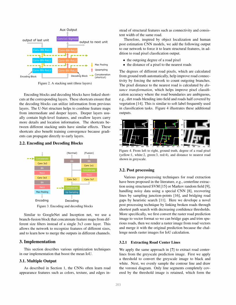
Figure 2. A stacking unit (three layers)

Encoding blocks and decoding blocks have linked short-

cuts at the corresponding layers. These shortcuts ensure that

the decoding blocks can utilize information from previous

layers. The U-Net structure helps to combine feature maps

from intermediate and deeper layers. Deeper layers usu-

ally contain high-level features, and swallow layers carry

more details and location information. The shortcuts be-

tween different stacking units have similar effects. These

shortcuts also benefit training convergence because gradi-

ents can propagate directly to early layers.

2.2. Encoding and Decoding Blocks

Conv 3x3

BN

ReLU

Conv 3x3

BN

ReLU

BN

Concatenate

Up-SamplingMax-Pooling

Concatenate

Concatenate

Conv 7x7

Conv 1x1

Conv 3x3

ReLU

BN

(Normal) (Fusion)

Encoding Decoding

Figure 3. Encoding and decoding blocks

Similar to GoogleNet and Inception net, we use a

branch-fusion block that concatenate feature maps from dif-

ferent size filters instead of a single 3x3 conv layer. This

allows the network to recognize features of different sizes,

and to learn how to merge the outputs in different channels.

3. Implementation

This section describes various optimization techniques

in our implementation that boost the mean IoU.

3.1. Multiple Output

As described in Section 1, the CNNs often learn road

appearance features such as colors, texture, and edges in-

stead of structural features such as connectivity and consis-

tent width of the same road.

Therefore, inspired by object localization and human

post estimation CNN models, we add the following output

to our network to force it to learn structural features, in ad-

dition to road pixel classfication output.

• the outgoing degree of a road pixel

• the distance of a pixel to the nearest roads

The degrees of different road pixels, which are calculated

from ground truth automatically, help improve road connec-

tivity by forcing the network to count outgoing branches.

The pixel distance to the nearest road is calculated by dis-

tance transformation, which helps improve pixel classifi-

cation accuracy where the road boundaries are ambiguous,

e.g., dirt roads blending into field and roads half covered by

vegetation [14]. This is similar to soft label frequently used

in classification tasks. Figure 4 illustrates these additional

outputs.

Figure 4. From left to right, ground truth, degree of a road pixel

(yellow:1, white:2, green:3, red:4), and distance to nearest road

shown in greyscale.

3.2. Post processing

Various post-processing techniques for road extraction

have been proposed in the literature, e.g., centerline extrac-

tion using structured SVM [15] or Markov random field [9],

handling noisy data using a special CNN [8], recovering

lines by sampling junction-points [16], and bridging road

gaps by heuristic search [11]. Here we develope a novel

post processing technique by linking broken roads through

shortest path search with decreasing confidence thresholds.

More specifically, we first convert the raster road prediction

image to vector format so we can bridge gaps and trim spu-

rious roads, then we render a raster image from road vectors

and merge it with the original prediction because the chal-

lenge needs raster images for IoU calculation.

3.2.1 Extracting Road Center Lines

We apply the same approach in [?] to extract road center-

lines from the greyscale prediction image. First we apply

a threshold to convert the greyscale image to black and

white. Next, we evenly sample the contour line and draw

the voronoi diagram. Only line segments completely cov-

ered by the threshold image is retained, which form the

203

road centerlines. We employ several optimization tweaks

for cleaner road networks, including trimming road stubs

and merging close intersections; see Fig. 5.

When rendering a raster image from road vectors, we

need to know the road width, calculated from the average

width along the road centerline using a dropoff threshold of

75% gray from the center.

Figure 5. Centerline extraction using voronoi diagram

3.2.2 Connecting Broken Roads

Connecting broken roads helps improve recall significantly.

Starting from a deadend in the vector road network ex-

tracted, we search possible connections to another existing

road using the shortest path algorithm. We assign the cost of

each pixel i as ci = −log[(pi + ε)/(1 + ε)], where pi is the

road classification probability of the pixel. This forces the

shortest path to prefer pixels with high probabilities of be-

ing roads, although not exceeding the threshold set in cen-

terline extraction step above. It also prefers road centerlines

instead of shortcuts along curved roads because centerlines

typically have higher prediction probabilities. To further

improve accuracy and speed, we apply shortest path search

in multiple iterations with decreasing thresholds. We also

set a maximum cost in each iteration so we only search a

certain range for connection; see Algorithm 1. Here U(s, δ)denotes the neighborhood of s with radius δ. The list of

decreasing threshold tk we use is {0.5, 0.2, 0.1, 0.05, 0.01}and δ is 100 pixels.

Fig.6 shows an example of the procedure. Areas in dif-

ferent colors represent the search ranges under different

thresholds. Each iteration decreases the threshold and there-

fore increases the search range. The iterative search result

in (F) is bbetter than a one-pass search in (B). It is also faster

because each iteration only searches a small range of pixels.

3.3. Hybrid loss function

The cross-entropy loss with our unbalanced training data

leads to slow convergence and low accuracy. We add the

Jaccard loss into our loss function L = Lce−λ logLjaccard,

where

Lce = −1

N

N∑

i=0

(y log y′ + (1− y) log (1− y′)) (1)

Ljaccard =1

N

N∑

i=0

yiy′

i

yi + y′i − yiy′i(2)

Algorithm 1 Threshold decreasing

Require: The topological graph of road map, Tn,m; The

predicted labels map, Pn,m; The thresholds list, tk;

Ensure: The gap-connected road map Q;

1: Q← T ;

2: for each t in tk do

3: for all 1-degree point s with another 1-degree point

exists in U(s, δ) do

4: P ′ ← threshold by range [tk, tk−1]5: ∆Q← PathSearch(P ′, s, t);6: Q← Q ∪∆Q;

7: end for

8: end for

9: return Q;

Figure 6. Connecting broken roads. A: original prediction; B: one-

pass search, C - E: different iterations with decreasing threshold;

F: final results.

Figure 7. Cross Entropy Surface Figure 8. Jaccard Surface

Here y and y′ mean the target and prediction vectors, re-

spectively, and λ is the weight of the Jaccard loss[18].

For cross entropy loss, the imbalance of sample points

(97%neg. vs 3%pos.) makes direction of gradient decreas-

ing toward the back conner (Fig.7), which leads to a local

optimum, especially in the early stage. The Jaccard loss ef-

fectively “lifts up” the back conner, and helps to avoid the

local optimum; see Fig. 8.

4. Experiments

Our experiments are performed on DeepGlobe dataset

[19]. Our network is trained using Keras with the Tensor-

204

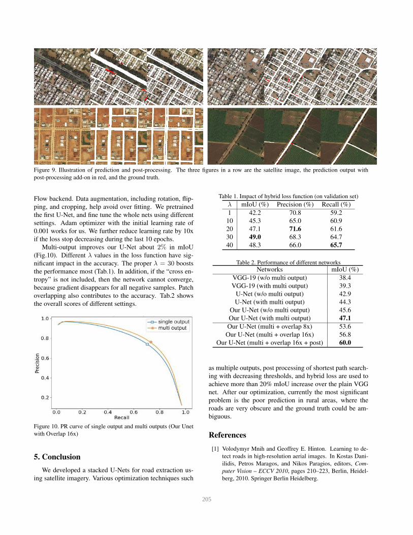
Figure 9. Illustration of prediction and post-processing. The three figures in a row are the satellite image, the prediction output with

post-processing add-on in red, and the ground truth.

Flow backend. Data augmentation, including rotation, flip-

ping, and cropping, help avoid over fitting. We pretrained

the first U-Net, and fine tune the whole nets using different

settings. Adam optimizer with the initial learning rate of

0.001 works for us. We further reduce learning rate by 10x

if the loss stop decreasing during the last 10 epochs.

Multi-output improves our U-Net about 2% in mIoU

(Fig.10). Different λ values in the loss function have sig-

nificant impact in the accuracy. The proper λ = 30 boosts

the performance most (Tab.1). In addition, if the “cross en-

tropy” is not included, then the network cannot converge,

because gradient disappears for all negative samples. Patch

overlapping also contributes to the accuracy. Tab.2 shows

the overall scores of different settings.

Figure 10. PR curve of single output and multi outputs (Our Unet

with Overlap 16x)

5. Conclusion

We developed a stacked U-Nets for road extraction us-

ing satellite imagery. Various optimization techniques such

Table 1. Impact of hybrid loss function (on validation set)

λ mIoU (%) Precision (%) Recall (%)

1 42.2 70.8 59.2

10 45.3 65.0 60.9

20 47.1 71.6 61.6

30 49.0 68.3 64.7

40 48.3 66.0 65.7

Table 2. Performance of different networks

Networks mIoU (%)

VGG-19 (w/o multi output) 38.4

VGG-19 (with multi output) 39.3

U-Net (w/o multi output) 42.9

U-Net (with multi output) 44.3

Our U-Net (w/o multi output) 45.6

Our U-Net (with multi output) 47.1

Our U-Net (multi + overlap 8x) 53.6

Our U-Net (multi + overlap 16x) 56.8

Our U-Net (multi + overlap 16x + post) 60.0

as multiple outputs, post processing of shortest path search-

ing with decreasing thresholds, and hybrid loss are used to

achieve more than 20% mIoU increase over the plain VGG

net. After our optimization, currently the most significant

problem is the poor prediction in rural areas, where the

roads are very obscure and the ground truth could be am-

biguous.

References

[1] Volodymyr Mnih and Geoffrey E. Hinton. Learning to de-

tect roads in high-resolution aerial images. In Kostas Dani-

ilidis, Petros Maragos, and Nikos Paragios, editors, Com-

puter Vision – ECCV 2010, pages 210–223, Berlin, Heidel-

berg, 2010. Springer Berlin Heidelberg.

205

[2] Alex Krizhevsky, Ilya Sutskever, and Geoffrey E Hinton. Im-

ageNet Classification with Deep Convolutional Neural Net-

works. NIPS, 2012.

[3] Pierre Sermanet, David Eigen, Xiang Zhang, Michael Math-

ieu, Rob Fergus, and Yann LeCun. OverFeat: Integrated

Recognition, Localization and Detection using Convolu-

tional Networks. arXiv.org, December 2013.

[4] Matthew D Zeiler and Rob Fergus. Visualizing and Un-

derstanding Convolutional Networks. In ECCV. Springer,

Cham, Cham, September 2014.

[5] Karen Simonyan and Andrew Zisserman. Very Deep Con-

volutional Networks for Large-Scale Image Recognition.

CoRR, 2014.

[6] Kaiming He, Xiangyu Zhang, Shaoqing Ren, and Jian Sun.

Deep Residual Learning for Image Recognition. In CVPR,

2016.

[7] Volodymyr Mnih and Geoffrey E. Hinton. Learning to detect

roads in high-resolution aerial images. In Computer Vision

- ECCV 2010 - European Conference on Computer Vision,

Heraklion, Crete, Greece, September 5-11, 2010, Proceed-

ings, pages 210–223, 2010.

[8] Volodymyr Mnih and Geoffrey E Hinton. Learning to Label

Aerial Images from Noisy Data. ICML, 2012.

[9] Gellert Mattyus, Shenlong Wang, Sanja Fidler, and Raquel

Urtasun. Enhancing Road Maps by Parsing Aerial Images

Around the World. ICCV, pages 1689–1697, 2015.

[10] Yin Wang. Scaling Maps at Facebook. In SIGSPATIAL,

2016. keynote.

[11] Gellert Mattyus, Wenjie Luo, and Raquel Urtasun. Deep-

RoadMapper - Extracting Road Topology from Aerial Im-

ages. ICCV, pages 3458–3466, 2017.

[12] E. Shelhamer, J. Long, and T. Darrell. Fully convolutional

networks for semantic segmentation. IEEE Trans. on PAMI,

39(4):640–651, April 2017.

[13] Olaf Ronneberger, Philipp Fischer, and Thomas Brox. U-

Net: Convolutional Networks for Biomedical Image Seg-

mentation. In Medical Image Computing and Computer-

Assisted Intervention – MICCAI 2015, pages 234–241.

Springer International Publishing, Cham, November 2015.

[14] Benjamin Bischke, Patrick Helber, Joachim Folz, Damian

Borth, and Andreas Dengel. Multi-Task Learning for Seg-

mentation of Building Footprints with Deep Neural Net-

works. CoRR, 2017.

[15] Elisa Ricci and Renzo Perfetti. Large Margin Methods for

Structured Output Prediction.

[16] Dengfeng Chai, Wolfgang Forstner, and Florent Lafarge. Re-

covering Line-Networks in Images by Junction-Point Pro-

cesses. CVPR, 2013.

[17] Xuemei Liu, James Biagioni, Jakob Eriksson, Yin Wang,

George Forman, and Yanmin Zhu. Mining large-scale, sparse

gps traces for map inference: Comparison of approaches. In

Proceedings of the 18th ACM SIGKDD International Con-

ference on Knowledge Discovery and Data Mining, KDD

’12, pages 669–677, New York, NY, USA, 2012. ACM.

[18] Maxim Berman, Amal Rannen Triki, and Matthew B

Blaschko. The Lovasz-Softmax loss: A tractable surrogate

for the optimization of the intersection-over-union measure

in neural networks. arXiv.org, May 2017.

[19] David Lindenbaum Guan Pang Jing Huang Saikat Basu

Forest Hughes Devis Tuia Ramesh Raskar Ilke Demir,

Krzysztof Koperski. DeepGlobe 2018: A Challenge to Parse

the Earth through Satellite Images. arXiv.org, 2018.

206