Stable long-term simulation of dynamically loaded elastomers
2
PAMM · Proc. Appl. Math. Mech. 8, 10501 – 10502 (2008) / DOI 10.1002/pamm.200810501 Stable long-term simulation of dynamically loaded elastomers Michael Groß and Peter Betsch ∗ Chair of Computational Mechanics, Department of Mechanical Engineering, University of Siegen, Paul-Bonatz-Str. 9-11, D-57068 Siegen, Germany A well-known problem in long-term simulations of flexible solid bodies is the restriction to small time steps of standard time integrators in order to obtain a stable simulation. One approach is to achieve exact energy conservation while simulating a nonlinear elastic body (see Reference [1] and the references therein). Additionally, total linear and total angular momentum is conserved for a free motion. This approach leads to a qualitatively improved solution, because the approximated time evolution exactly fulfills the same physical laws as the exact time evolution. Incorporating energy dissipation, the energy conserving time integration is extended to an energy consistent time integration. It turned out that such an energy consistent time integration is also of great advantage when computing finite motions of flexible solid bodies with material dissipation (see References [2, 3]). This paper points out that an energy consistent time discretisation is also advantageous for dynamic finite deformation thermoviscoelasticity under dynamic loads. c 2008 WILEY-VCH Verlag GmbH & Co. KGaA, Weinheim 1 The motivation One range of application of elastomers in dynamical systems are elastomer disks and pins in flexible couplings. In order to perform a long-term analysis of flexible elements in couplings, time integration algorithms are necessary, which are convenient for long-term simulations of dynamically loaded elastomeric materials. Recall that an elastomer has the ability to save non- linear strain energy during a cyclic loading (elastic behaviour), however, owing to internal friction internal energy dissipates in each cycle, and leads to a self-heating of the flexible element (thermoviscous behaviour). Since self-heating of elastomeric materials leads to an accelerated ageing, numerical simulations of flexible couplings ought to calculate the exact dissipation. Additionally, time integration algorithms have to be numerically stable in order to be convenient for long-term simulations. 2 The inherently energy-consistent method From the balance of kinetic energy rate, stress power and external mechanical power, we derive the local form of the equations of motion. The postulate of a non-negative total production of entropy, expressed by the balance of total entropy and entropy input, leads to the local form of the entropy balance. As viscoelastic potential, we assume an isotropic free energy with a symmetric second-order tensor as internal variable. The non-negative thermal dissipation in the entropy balance arise from an isotropic heat flux, linear in the temperature gradient (Fourier’s law). The non-negative internal dissipation follows from a Mandel stress tensor, which is linear in the corresponding viscous deformation rate tensor. We obtain an independent nonlinear differential equation representing a viscous evolution equation. The equations of motion relate conservation laws to a free moving and mechanically unloaded body. The total linear momentum function is conserved for a free translational motion, and the total angular momentum function is conserved for a free rotational motion. For the sum of kinetic and relative internal energy, which we call the relative total energy, there also exists a decay estimate without loads. This estimate can be interpreted as a stability estimate of the differential equations. Further, this estimate yields appropriate weak forms of the differential equations in the following manner: Considering the change of kinetic energy along a continuous time curve, in a first step, we obtain the weak form of the first equation of motion, and in a second step, we obtain the weak form of the second equation of motion. In this way, we arrive at continuous Galerkin forms in time, because the time derivatives of the independent variables are admissible test functions. On the other hand, the change of relative internal energy along a continuous time curve -15 -10 -5 0 5 10 15 20 25 30 35 40 45 -15 -10 -5 0 5 10 15 295 300 305 310 x y Current temperature 0 5 10 15 0 20 40 60 80 100 120 140 160 180 200 Time Stability estimate 0 5 10 15 20 -1000 0 1000 2000 3000 4000 5000 6000 P1 P2 P3 Time Linear momentum 0 5 10 15 20 -2 -1.8 -1.6 -1.4 -1.2 -1 -0.8 -0.6 -0.4 -0.2 0 x 10 5 L1 L2 L3 Time Angular momentum 0 5 10 15 6 6.1 6.2 6.3 6.4 6.5 6.6 6.7 x 10 4 Time Relative total energy Fig. 1 Simulation with (bi)linear finite elements, using the inherently energy-consistent method. Before t =5, the time step size is h n =0.01, and behind the dotted line, we have h n =0.1. The ring is stiff and has a heat leak in a small range of the outside diameter. ∗ Corresponding author: e-mail: [email protected], Phone: +49 271 740 2224, Fax: +49 271 740 2436 c 2008 WILEY-VCH Verlag GmbH & Co. KGaA, Weinheim
-
Upload
michael-gross -
Category
Documents
-
view
212 -
download
0
Transcript of Stable long-term simulation of dynamically loaded elastomers
PAMM · Proc. Appl. Math. Mech. 8, 10501 – 10502 (2008) / DOI 10.1002/pamm.200810501
Stable long-term simulation of dynamically loaded elastomers
Michael Groß and Peter Betsch ∗
Chair of Computational Mechanics, Department of Mechanical Engineering, University of Siegen, Paul-Bonatz-Str. 9-11,D-57068 Siegen, Germany
A well-known problem in long-term simulations of flexible solid bodies is the restriction to small time steps of standard timeintegrators in order to obtain a stable simulation. One approach is to achieve exact energy conservation while simulating anonlinear elastic body (see Reference [1] and the references therein). Additionally, total linear and total angular momentumis conserved for a free motion. This approach leads to a qualitatively improved solution, because the approximated timeevolution exactly fulfills the same physical laws as the exact time evolution. Incorporating energy dissipation, the energyconserving time integration is extended to an energy consistent time integration. It turned out that such an energy consistenttime integration is also of great advantage when computing finite motions of flexible solid bodies with material dissipation(see References [2, 3]). This paper points out that an energy consistent time discretisation is also advantageous for dynamicfinite deformation thermoviscoelasticity under dynamic loads.
c© 2008 WILEY-VCH Verlag GmbH & Co. KGaA, Weinheim
1 The motivation
One range of application of elastomers in dynamical systems are elastomer disks and pins in flexible couplings. In order toperform a long-term analysis of flexible elements in couplings, time integration algorithms are necessary, which are convenientfor long-term simulations of dynamically loaded elastomeric materials. Recall that an elastomer has the ability to save non-linear strain energy during a cyclic loading (elastic behaviour), however, owing to internal friction internal energy dissipatesin each cycle, and leads to a self-heating of the flexible element (thermoviscous behaviour). Since self-heating of elastomericmaterials leads to an accelerated ageing, numerical simulations of flexible couplings ought to calculate the exact dissipation.Additionally, time integration algorithms have to be numerically stable in order to be convenient for long-term simulations.
2 The inherently energy-consistent method
From the balance of kinetic energy rate, stress power and external mechanical power, we derive the local form of the equationsof motion. The postulate of a non-negative total production of entropy, expressed by the balance of total entropy and entropyinput, leads to the local form of the entropy balance. As viscoelastic potential, we assume an isotropic free energy with asymmetric second-order tensor as internal variable. The non-negative thermal dissipation in the entropy balance arise froman isotropic heat flux, linear in the temperature gradient (Fourier’s law). The non-negative internal dissipation follows froma Mandel stress tensor, which is linear in the corresponding viscous deformation rate tensor. We obtain an independentnonlinear differential equation representing a viscous evolution equation. The equations of motion relate conservation lawsto a free moving and mechanically unloaded body. The total linear momentum function is conserved for a free translationalmotion, and the total angular momentum function is conserved for a free rotational motion. For the sum of kinetic and relativeinternal energy, which we call the relative total energy, there also exists a decay estimate without loads. This estimate canbe interpreted as a stability estimate of the differential equations. Further, this estimate yields appropriate weak forms of thedifferential equations in the following manner: Considering the change of kinetic energy along a continuous time curve, in afirst step, we obtain the weak form of the first equation of motion, and in a second step, we obtain the weak form of the secondequation of motion. In this way, we arrive at continuous Galerkin forms in time, because the time derivatives of the independentvariables are admissible test functions. On the other hand, the change of relative internal energy along a continuous time curve
−15 −10 −5 0 5 10 15 20 25 30 35 40 45−15
−10
−5
0
5
10
15
295
300
305
310
x
y
Current temperature
0 5 10 150
20
40
60
80
100
120
140
160
180
200
Time
Stab
ility
estim
ate
0 5 10 15 20−1000
0
1000
2000
3000
4000
5000
6000
P1P2P3
Time
Lin
ear
mom
entu
m
0 5 10 15 20−2
−1.8
−1.6
−1.4
−1.2
−1
−0.8
−0.6
−0.4
−0.2
0x 10
5
L1L2L3
Time
Ang
ular
mom
entu
m
0 5 10 156
6.1
6.2
6.3
6.4
6.5
6.6
6.7x 10
4
Time
Rel
ativ
eto
tale
nerg
y
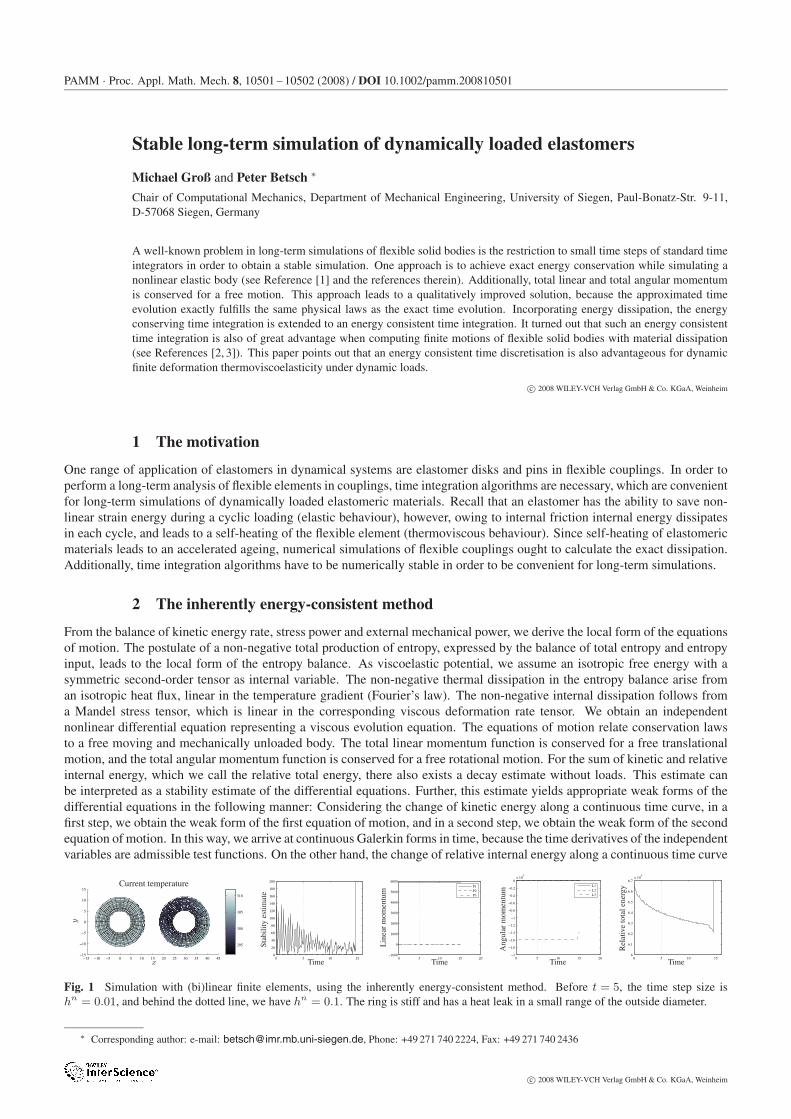
Fig. 1 Simulation with (bi)linear finite elements, using the inherently energy-consistent method. Before t = 5, the time step size ishn = 0.01, and behind the dotted line, we have hn = 0.1. The ring is stiff and has a heat leak in a small range of the outside diameter.
∗ Corresponding author: e-mail: [email protected], Phone: +49 271 740 2224, Fax: +49 271 740 2436
c© 2008 WILEY-VCH Verlag GmbH & Co. KGaA, Weinheim
10502 Sessions of Short Communications 07: Coupled problems
yields the weak form of the local entropy balance. We obtain a discontinuous Galerkin form in time with an energy-basedjump term, because the relative temperature is the admissible test function. The definition of the internal dissipation leadsto a spatially local continuous Galerkin form in time for the internal variable. Therefore, multiplying the viscous evolutionequation with the viscous deformation rate tensor, the internal dissipation coincides with a positive-definite quadratic form. Aphysically meaningful stopping criterion of the local iterative solution procedure is to check this identity after each iteration.The convergence of the global iterative solution procedure is stopped if the Frobenius norm of the global residual is less than asmall tolerance (absolute criterion). However, this thermo-mechanically uncoupled global criterion is affected by bad scaling,which prevents to choose a large time step where the dissipation is high (see at the beginning of the simulation in Fig. 1).Now, we consider a free flying and stiff elastomeric ring, calculated by this inherently energy-consistent method. However,the stability estimate is not exactly fulfilled, and the relative total energy is not steady decreasing. Further, a greater timestep size leads to a divergence of the algorithm, which is induced by an artificial increasing dissipation. Nevertheless, themomentum maps are conserved till the algorithm diverged.
3 The exactly energy-consistent method
The origin of this behaviour lies in the fact that the inherently energy-consistent method is exactly energy-consistent onlywith exact integration. In order to retain the energy consistency with numerical integration, we adjust the energy transferto the numerical integration as follows: The total linear momentum is already conserved, and the total angular momentumconservation only requires a certain number of Gauss points as well as a symmetrically approximated Kirchhoff stress tensor.Note that the change of kinetic energy by mechanical work is calculated exactly by this numerical integration rule. However,the change of relative internal energy by work and total dissipation generally cannot be calculated exactly by using numericalintegration. First, we correct the energy transfer with a coupling stress power by introducing an additional term in the weakform of the second equation of motion. Second, the distinct number of Gauss points in the weak forms is balanced by acoupling dissipation in the weak form of the entropy evolution equation. These enhanced weak forms allows to use the balance
0 50 100 150 2000
0.1
0.2
0.3
0.4
0.5
0.6
0.7
0.8
0.9
1x 10
−8
Time
Apr
iori
stab
ility
estim
ate
0 50 100 150 2006
6.1
6.2
6.3
6.4
6.5
6.6
6.7x 10
4
Time
Rel
ativ
eto
tale
nerg
y
0 50 100 150 200−1000
0
1000
2000
3000
4000
5000
6000
P1P2P3
Time
Tota
llin
ear
mom
entu
m
0 50 100 150 200−2
−1.8
−1.6
−1.4
−1.2
−1
−0.8
−0.6
−0.4
−0.2
0x 10
5
L1L2L3
Time
Tota
lang
ular
mom
entu
m
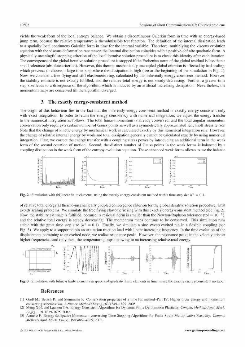
Fig. 2 Simulation with (bi)linear finite elements, using the exactly energy-consistent method with a time step size hn = 0.1.
of relative total energy as thermo-mechanically coupled convergence criterion for the global iterative solution procedure, whatavoids scaling problems. We simulate the free flying elastomeric ring with this exactly energy-consistent method (see Fig. 2).Now, the stability estimate is fulfilled, because its residual norm is smaller than the Newton-Raphson tolerance (tol = 10−8),and the relative total energy is steady decreasing. The momentum maps continue to be conserved. This simulation runsstable with the great time step size (hn = 0.1). Finally, we simulate a sine sweep excited pin in a flexible coupling (seeFig. 3). We apply to a supported pin an excitation traction load with linear increasing frequency. In the time evolution of thedisplacement pertaining to an excited node, we realise resonance peaks. However, the resonance peaks in the velocity arise athigher frequencies, and only then, the temperature jumps up owing to an increasing relative total energy.
tttt
Θ∞
Θ∞0 1 2 3 4 5
−1500
−1000
−500
0
500
1000
1500
Time
Exc
itatio
ntr
actio
nlo
ad
0 20 40 60 80
−0.4
−0.3
−0.2
−0.1
0
0.1
0.2
0.3
0.4
Time
Dis
plac
emen
t
0 20 40 60 80−25
−20
−15
−10
−5
0
5
10
15
20
25
Time
Vel
ocity
0 20 40 60 80
10
12
14
16
18
20
22
Time
Rel
ativ
ete
mpe
ratu
re
Fig. 3 Simulation with bilinear finite elements in space and quadratic finite elements in time, using the exactly energy-consistent method.
References
[1] Groß M., Betsch P., and Steinmann P. Conservation properties of a time FE method–Part IV: Higher order energy and momentumconserving schemes. Int. J. Numer. Methods Engng., 63:1849–1897, 2005.
[2] Meng X.N. and Laursen T.A. Energy Consistent Algorithms for Dynamic Finite Deformation Plasticity. Comput. Methods Appl. Mech.Engrg., 191:1639-1675, 2002.
[3] Armero F. Energy-dissipative Momentum-conserving Time-Stepping Algorithms for Finite Strain Multiplicative Plasticity. Comput.Methods Appl. Mech. Engrg., 195:4862-4889, 2006.
c© 2008 WILEY-VCH Verlag GmbH & Co. KGaA, Weinheim www.gamm-proceedings.com