Stability of Rock Mass* by

T. Ramamurthy**

INTRODUCTION My involvement in soil mechanics has been for quite some years, right from the beginning of my career.

I was fascinated by soil mechanics activity when I made a casual visit to the Andhra Pradesh Engineering Research Laboratories. I joined their Soil Mechanics Laboratory to make a career for myself.

I was contemplating to deliver this lecture on one of the following aspects ...

(i) Strength and deformation response of cohesionless soils in general stress system including plane strain,

(ii) crushing phenomena and response of cohesionless soils under high stresses including modelling of rockfills, or

(iii) stability of soil s_lopes and some important considerations in the design of high earth and rockfill dams.

During the last few years, at liT Delhi, a base has been laid in the area of rock mechanics. In view of this I have accepted the advice of my colleagues to deliver this IGS Lecture on rock mechanics. Some results are beginning to come out of our research; I therefore choose "stability of rock mass" as the topic of this Lecture. I will confine myself to the strength aspect of intact- isotropic and anisotropic rocks, rock masses, to the stability of rock slopes and underground openings in squeezing grounds. Characterization of rocks and rock masses is essential for any realistic analysis of rock slopes, foundations of dams, or rock mass around tunnels. Numerous problems are being faced during open excavations in rock mass. On many occasions work in underground excavations had to be stopped for months in highly squeezing grounds in the Himalayas and therefore the relevance of the topic is being emphasized in this lecture.

Probably this is the first, in the series of lectures, on rock mechanics to be delivered in the country and I do hope many more will soon follow and generate considerable research activity. For the numerous proolems we are facing both in hard and soft rock formations in this country, we alone have to find solutions to them by our active involvement.

Rock mechanics activity in terms of teaching, research and practice has been a recent phenomenon in India. Teaching at the post-graduate level was first started through an elective course at the Indian Institute of Science in 1964. During 1972, the subject was being taught as an elective only at four Institutes. To the undergraduates it was first introduced at the Indian Institute of Technology, Delhi, during 1971 and to the post­graduates, a set of courses in Rock Mechanics was offered for minor specialization during 1976. In 1977 at this Institute, a fullfledged master's programme in rock mechanics was started for civil engineers for the first time in this country. This programme has been opened to mining engineers in July, 1985 and is the only programme currently being offered.

Research in rock mechanics has been considerably slow. Reasonably good facilities now exist at some of the educational institutions like Banaras Hindu University, Indian School of Mines, Regional Engineering College, Kurukshetra, and to some extent at the University of Roorkee and the Indian Institutes of Technology located at Bombay and Kanpur. Some of the national research institutes, like Central Soil and Materials Research Station, Central Mining Research Institute, National Geophysical Research Institute and Central Water and Power Research Station have acquired good facilities for testing and research over the years. State research laboratories have also built up some testing facilities and started some research activities through the funds provided by the Central Board of Irrigation and Power. Of late, research publications from this country have been increasing in number both at the national and international levels.

At liT Delhi we have been steadily building research facilities in rock mechanics in terms of laboratory testing and computer programmes. Apart form various laboratory testing equipment some of the important

*Eigth IGS Annual Lecture delivered on the occasion if its 27th Annual General Session held at Roorkee, India.

**Professor and Head. Civil Engineering Department, Indian Institute of Technology, New Oelhi-110016, India.

221

facilities that are available are :

(i) High pressure triaxial equipment to test rock specimens under confining pressures upto 1400 kg/ cm2

- it includes volume measuring system as well;

(ii) A biaxial loading frame for testing rock specimens upto 70x70x70 em size with maximum loading upto 500 t vertical and 100 t horizontal with electrical and manual loading and unloading and rate control facility;

(iii) Geomechanics modelling facility to test scaled models (3 m long and 1 m high) for the study of deformation pattern and failure modes for underground and open excavations and also stability of fundations of dams;

(iv) Data logging system connected to LVDTs and load cells and pressure transducers; and

(v) Field testing facilities to load .upto 500 t.

ROCK AND ROCK MASS

An intact rock is considered to be an aggregate of minerals without any structural defects. Such rocks are treated as isotropic, homogeneous and continuous. A rock mass includes structural features induced in it by the force field of its physical environment. These features viz., bedding planes, shear planes, fault planes, joint planes and fracture planes, render rock mass anisotropic, nonhomogeneous and discontinuous. Heavily fractured rock and intact rock are often treated as continum. Because of the size and persistence or otherwise of the structural defects, testing of specimens of rock mass in the laboratory has become restrictive in practice. To a large extent, more than in the case of soils, greater relevance is placed on insitu evaluation of the response of rock mass in the anticipated stress range and stress field. Estimation of relevant parameters for the design of civil and mining engineering works is of paramount importance. Sometimes comprehensive data collection both from field and laboratory is carried out primarily to perform a realistic analysis of the rock mass, that is, to predict its deformational response and stability.

Strength of intact rock is influenced mainly by (i) geological, (ii) lithological, (iii) physical,(iv) mechanical and (v) environmental factors, as presented in Table 1.

Geological

Geological Age

Weathering and other alterations

TABLE.1

FACTORS AFFECTING INTACT ROCK STRENGTH

INTACT ROCK STRENGTH

Lithological

Mineral Composition

Cementing Material

Texture and Fabric Anisotropy

Physical

Density/ specific gravity

Void Index

Porosity

Mechanical

Specimen preparation

Specimen geometry

End contact/ end restraint ·Type of testing machine Rate of loading

STRENGTH CRITERIA FOR INTACT ROCKS

Environmental

Moisture content

Nature of pore fluids

Temperature

Confining Pressure

Under a given situation, geological, lithological, physical, environmental and most of the mechanical aspects remain constant and the influence of confining pressure is predominant. The effect of confining pressure on the strength of intact rock has been investigated extensively starting with von Karman (1911) who· conducted pioneering experiments on Carrara marble in copper jackets and observed a nonlinear variation of strength with confining pressure. All the subsequent investigations conducted to study the influence of confining pressure

222

confirm this nonlinear response. An important aspect of rock behaviour under triaxial condition is the change in behaviour from brittle to ductile nature at high confining pressures (Grigg 1936, Donath 1970, Magi 1972, Hoshi no eta/. 1972, Ramamurthy and Goel1973).

For argillaceous sandstone and siltstone, brittle to ductile transition occurs under confining pressure range of 1000-3000 kg/cm2 (Handin and Hager 1957, Hoshino ~t a/., 1972). For rock salt and gypsum this pressure is as low as 200-400 kg/cm2 • This transition was usually observed when o,fo

3 is in the range of 3 to 5

(Schwarz 1954, Magi 1965). A rare exception to this nonlinearity is in the case of highly crystalline rocks like quartzite and granite which tend to exhibit linear response. The well known Navier-Coulomb theory based on maximum shear stress criterion predicts a linear behaviour. The classical Griffith's criterion based on failure of rocks in tension predicts to some extent a nonlinear response. However, these classical theories, though simple in concept and also in use, fail to predict rock behaviour universally. Hence a need has beenfeltto develop a failure criterion applicable to most rock types.

To overcome this inadequacy, an empirical power law was suggested by Murrell (1968) as

o 1 = oc + B(oJA

or

-r=-r +bo 8

0 n

In the non-dimensional form these equations may be written as

( ~) = 1 + B (~( and

T - To = K(~f o;,

where A, B, K, a and b are material constants,

-r = shear strength at failure,

-r0

=shear strength at zero normal stress o",

oc = uniaxial compressive strength, and

o1

& o3

=major and minor principal stresses.

... (1)

... (2)

... (3)

... (4)

An alternate form of this power law was suggested by Hoek (1968) in terms of maximum shear stress and associated normal stress as

"[m - To D ( :: f =

where Oc

... (5)

01 - 03 "[m = om =

2

and C and Dare material constants.

For sandstones D = 0.76 and C = 0.85; similar values for other rock types are not available.

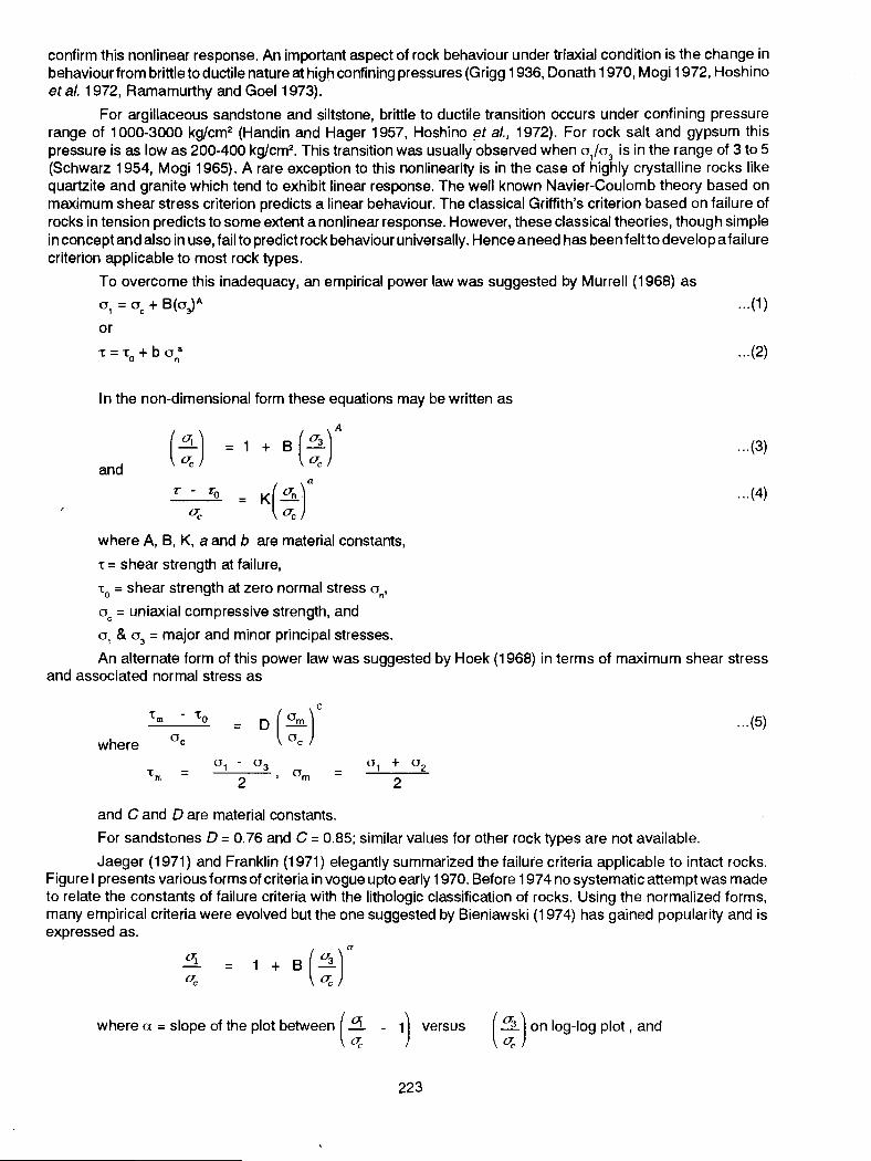
Jaeger (1971) and Franklin (1971) elegantly summarized the failure criteria applicable to intact rocks. Figure I presents various forms of criteria in vogue upto early 1970. Before 197 4 no systematic attempt was made to relate the constants of failure criteria with the lithologic classification of rocks. Using the normalized forms, many empirical criteria were evolved but the one suggested by Bieniawski (1974) has gained popularity and is expressed as.

where a = slope of the plot between ( ~ - 1) versus q.

223

( ~ ) on log-log plot , and

(a) (b) (c) (d)

FIGURE 1 Failure Criteria : (a) Coulomb, (b) Poncelet, (c) Griffith, (d) Power law ~Jaeger 1971)

8 = a material constant.

From a study of a range of South African rocks, Bieniawski had the distinction of linking up the contants of the failure criterion with the lithology of some rocks. He suggested that

of

a= 0.75 for all rock types

and 8 = 3.9 for siltstone and sandstone,

4.0 for sandstone,

4.5 for quartzite, and

5.0 for norite

Based on test results of four rock types, Brook (1979) modified Hoek's expression (1968) to take the form

11

.!ill_ = A ( {Tm )

o;. ({, ... (7}

Conforming to non-linear response of strength with confining pressure through trial and error process, Hoek and Brown (1980) suggested the following equation,

range.

1

o 1 = o3 + (moco3 + so~F ... (8)

where m and s are material parameters; s = 1 for intact rocks and m depends on rock type and has a wide

Yudbir eta/., {1983} gave a general form to Bieniawski's expression as

!1. = A+ B(03)a o;: oc

where a= slope of plot between ( ~ _ Aland ( ~) on log-log scale,

8 =material constant, and

A= dimensional pa;ameter which depends on rock quality; for intact rocks its value is unity.

Based on very limited data they proposed in the lines of Bieniawski a value of

8 = 2 for tuff, shale and limestone,

3 for siltstone and mudstone,

4 for sandstone, quartzite, and

224

... (9)

5 for norite and granite.

When the analysis of test data was carried out by adopting the criteria referred to in the foregoing sometimes significant deviations were observed suggesting the need for developing a more realistic criterion to be applicable at least in the first instance to intact rock, with a possibility of extending it to estimate rock mass strength. .,

PROPOSED STRENGTH CRITERION

In order to develop a simple mathematical expression which would enable prediction of strength sufficiently accurate not only for intact, but also of anisotropic rocks and fractured rock masses covering the entire brittle and ductile regions, an attempt has been made through Mohr-Coulomb failure criterion (Rao, 1984, Ramamurthy, Rao and Rao 1985 and Rao, Rao and Ramamurthy, 1985) as detailed hereunder:

As per Mohr-Coulomb criterion,

(u1 ~ o) = 2 c cos¢+ {o, + o) sin¢

where c =cohesion intercept, and

¢ = friction angle.

By normalising and rearranging, Eq. 10 be written as

2 c cos¢ 2 sin¢ +

lT3 (1 - sin¢) 1- sin¢

2 c cos¢ The term 1 _ sin¢ is equal tot\ (unconfined compressive strength when o 3=0.

therefore, 0 i - 03 Oj

= q + 03

2 sin¢ 1- sin¢

o;, (1 + .5._ . 2 si~¢ ] Oj q 1- Sin¢·

... (1 O)

... (11)

To take care of the variations inc and <I> with increase of confining pressure o3

and also to account for the non-linear behaviour, Eq. 12, is modified as a

( 0 ~ 03 ) = B ( ~ ) ... (13}

where 8 = rock material constant; function of rock type and quality; and

u = slope of plot between oc

and ~· on log-log plot.

The above expression is applicable for all values of o3>0.

To establish the applicability of this expression, initially four sandstones selected from different geological formations ranging from the Vindhyans to recent Siwalik, were tested (Rao, 1984) using simple triaxial cell (Ramamurthy, 1975). These sandstones were

(i) Kota sandstone, belonging to Bhander series of Upper Vindhyans (600 m.y.),

(ii) Singrauli sandstone, belonging to Purewa bottom series of Raniganj group of the Gondwana system (150 m.y.).

(iii) Jhingurda sandstone, Singrauli coal fields, belonging to Purewa top series of Raniganj group of the Gondwana system (150 m.y.). and

225

20.0·

10.0

5.0

6 --C")

0 I ...... 0 - 1.0

0.5 1.0 5.0

Oc/03

Data From 1. Hardshale (Hoshino et. al. , 1972) 2. Joban claystone ( ,,

) 3. Akitashale ( , ) 4. Repetto c. st. (Handin & Hager 1957) 5. tuff c. st. (Hoshino et. al. 1972 ) 6. Grey stone ( ,, ) 7. Silt stone ( II ) 8. Shale ( II ) 9. Black shale ( II ) 10. Tuff c. st. ( ,, ) 11. Tuff ( " ) 12. Loess. (Matalucci et. al. ' 1970)

c. st = Clay stone

10.0 50.0

FI<;URE. 2 Plot of Proposed Criterion for Argillaceous Rocks

(iv} Jam rani sandstone from a hydel project, U .P. belonging to the lower Siwalik of eastern Himalayas (25 m.y.).

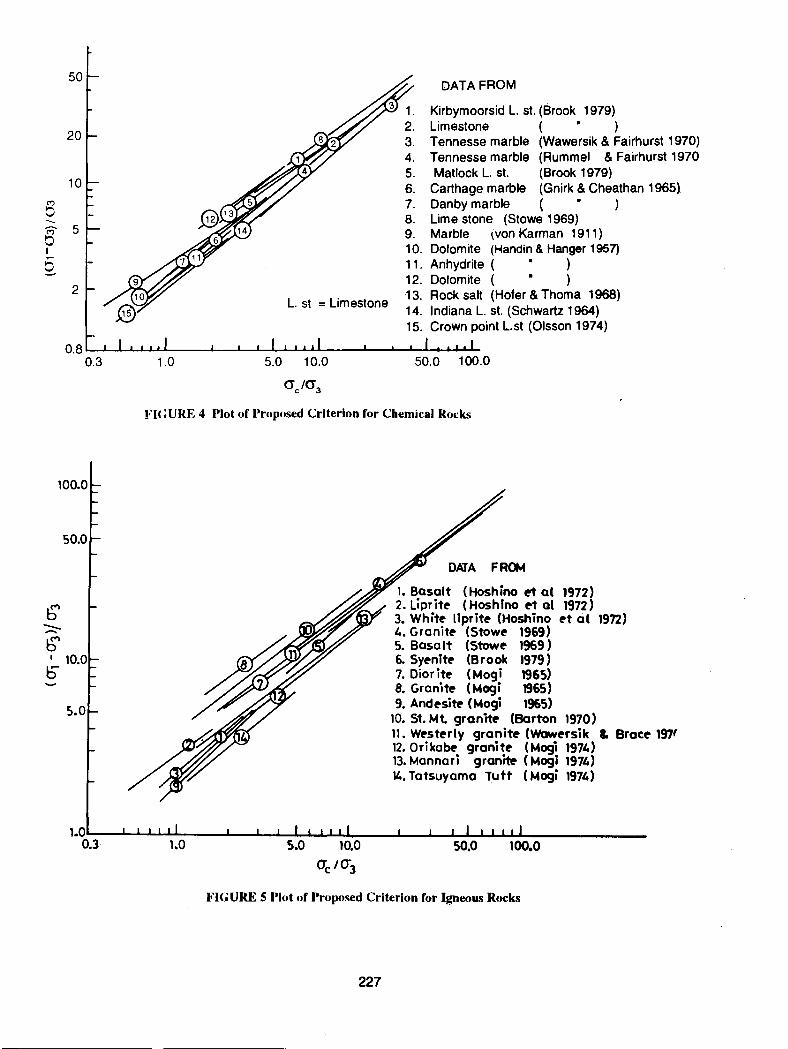
In addition to the data of these four sandstones, similar data of 80 different rock types published in the literature were analysed. These include sedimentary (argillaceous, arenaceous, and chemical), metamorphic and igneous rocks. Plot of the data in terms of (o, - oJ/o

3 versus ojo

3 for argillaceous rocks (shales 1.nd slates),

arenaceous (sandstone and quartzite), chemical (limestone, dolomite, anhydrite, rock salt and marble) and

30

Data From 10 1. Berea s. st. (Gnirk & Cheathan 1965 )

2. Grey s. st. (Hoshino et al. 1972) 3. Pottsvilles s. st. (Schwartz 1964) 4. Sandstone (Hoshino et al. 1972) 6 5. Grey s. st ( ) 6. Bandera s. st (Wilhelmi & Sometion 1967) 6 5

7. Boise s. st ( q )

8. Grey s. st ( Hoshino et al. 1972) 9. Oshima s. st. ( " )

I

.§. 10. Pniowek s. st. (Kwasniewski 1983) 11. Pniowek s. st. ( " ) 12. Quartzite ( Hoshino et al, 1972) 13. Berea s. st . ( Aldrich 1969 )

s. st = Sandstone

0.5 L---L--...J....-L..J-L..U.--...I..---'---'--:L:-.L..J...~=----L---J.--J.~~'""'7,~ 0.2 0.5 1.0 5.0 10

Oc/03

FIGURE 3 Plot of Proposed Criterion for Arenaceous Rocks

226

6 'M b I

§_

50

20

10

5

2 L. st = Limestone

DATA FROM

Kirbymoorsid L. st. (Brook 1979) Limestone ( ) Tennesse marble (Wawersik & Fairhurst 1970) Tennesse marble (Rummel & Fairhurst 1970 Matlock L. st. (Brook 1979)

Carthage marble (Gnirk & Cheathan 1965) Danby marble ( ) Lime stone (Stowe 1969) Marble tvon Karman 1911) Dolomite (l-olandin & Hanger 1957) Anhydrite ( ) Dolomite ( ) Rock salt (Hofer & Thoma 1968) Indiana L. st. (Schwartz 1964) Crown point L.st (Olsson 1974)

o.a~~~~LL----~~~~-LLL~----~~~~~~u-

0.3 1.0 5.0 10.0 50.0 100.0

FI<;URE 4 l,lot of Proposed Criterion for Chemical Rocks

DATA FROM

1. Basalt (Hoshino eot at 1972) 2. Liprit~ ( Hoshlno eot at 1972) 3. Whit~ llprit~ (Hoshino ~t at 1972) 4. Granit~ (Stow~ 1969) 5. Basalt (Stow~ 1969) 6. Sy~nit~ (Brook 1979) 7. Diorit~ (Mogi 1965) B. Grani~ (Mogi 1965) 9. And~sit~ (Mogi 1965)

10. St. Mt. granite- (Barton 1970) 11. W~st~rly granite- (WOw~rsik & Brae~ 197' 12. Orika~ granit~ (Mogi 1974) 13. Mannari gran~ ( Mogi 1974) 14. Tatsuyama Tuft ( Mogi 1974)

1-0~___. ........... ....Io....L~:---~----1'--L..::JL.:-L-..L.J...U.-:---....L...----IL...-.L....I-L.'-L..LL------0.3 1.0 5.0 10.0 50.0 100.0

O'c 10'3

FIGURE 5 Plot of Proposed Criterion for Igneous Rocks

227

50

20

(¥)

0 10 -

2

e Kota sandstone ( B = Oo) tJ. Jamra11i sandstone a Singrauli sandstone o Jhingurda sandstone

0.5 1.0 5.0 10.0

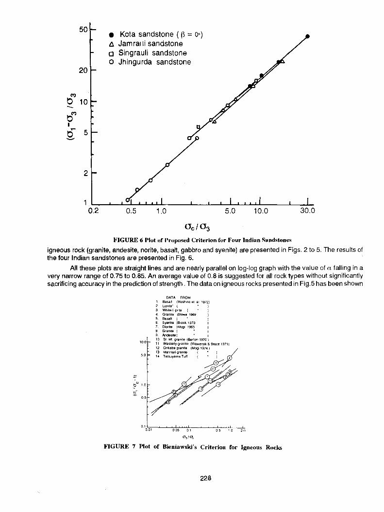
FIGURE 6 Plot of Proposed Criterion for Four Indian Sandstones

30.0

igneous rock (granite, andesite, norite, basalt, gabbro and syenite) are presented in Figs. 2 to 5. The results of the four Indian sandstones are presented in Fig. 6.

All these plots are straight lines and are nearly parallel on log-log graph with the value of a falling in a very narrow range of 0.75 to 0.85. An average value of 0.8 is suggested for all rock types without significantly sacrificing accuracy in the prediction of strength. The data on igneous rocks presented in Fig.5 has been shown

DATA FROM 1. Basalt (Hosh•no et al 1 972) 2 L1pnte" ( ) 3 White Liprite ( ) 4. Gran1te (Stowe 1969 )

5. Basall I I 6 Syenite (Brook 1979 ) 7. D1orite ( Mog• 1965 ) 8. Gramte ( • ) 9. Andesrte I I

10.0 10 St MI. gran1te (Ban on 1970 ) 11. Westerly gran•te (Wawers•k & Brace 1971) 12. Onkabe gramte (Mog1 1974)

5.0 1 !3. Mannari granite ( 14 Tatsuyama Tuff (

0, ~~~-'::-':-:'--'~--~~__.__j~_._.__L-...L. 0.01 0 05 0 1 0 5 1 0 2 o

FIGURE 7 Plot of Bieniawski's Criterion for Igneous Rocks

228

'E 0 -0> ~

0 .c ..... 0>

a5 800 ..... ..... (/)

~ ::J

"(ij u.

200

Experimental observation

0 Kota sandstone ( B = Qo) D. Jarilrani sandstone 0 Singrauli sandstone X Jhingurda sandstone

Proposed criterion Hoek- Brown

Magi transition _ --(01=3.403) --------- )( ~~~~-~-~~---

80 100 120

Confining pressure, () 3

kg/cm2

140

FI<;URE 8 Comparison Between Predicted and Measured Strength of Sandstones

in Fig. 7, as per Bieniawski's criterion to emphasise that definite values cannot be assigned to constants in Eq. 6. The values of a obtained from Bieniawski's expression vary over a wide range, i.e. from 0.4 to 1 .2. These values vary from one rock group to another and also even within the same rock group. Therefore, the assumption of a constant value of a from such wide variation is difficult to justify.

Using a constant value of a= 0.8 and the values of strength (uc) and o, for various value of o 3 , the values of Bwere calculated from Eq. 13. These values of Bforthefoursand~tones fall in a close range from 2.13to 2.69. Adopting s= 1 in Hoek-Brown criterion (Eq. 8), the values of m were estimated. The values of m vary widely from 1.42to 13.26 (Table2), whereas the suggested values of mforsuch rocks by Hoek and Brown (1980) is 15. Table 2 also presents the values of coefficient of determination ( r2

). These values of the coefficient are better for the proposed criterion than that for Hoek-Brown criterion suggesting definite advantage of the proposed criterion. A good agreement between the experimental results and proposed criterion is also reflected in Fig. 8.

A wide scatter in the values of m for different groups of rocks was observed and is indicated in Table3, along with the values suggested by Hoek and Brown (1980).

Table 4 has been prepared from test results (as an illustration) on Indiana limestone (Schwartz, 1964). The values of Band mare listed for different confining pressures. The values of 8 are nearly same but the values of m vary considerably over the range of confining pressures of 7.03 to 562.40 kg/cm2 The values of m decrease

229

TABLE 2

PARAMETERS EVALUATED FOR SANDSTONES

Rock Type Proposed Criterion Hoek-Brown Criterion

B (a= 0.8)

Kota sandstone 13= 0°

Jamrani sandstone

Singrauli sandstone

Jhingurda sgndstone

*Calculated from the triaxial test data

2.6900

2.5299

2.6286

2.1373

0.999 903.31

0.972

0.998

0.955

TABLE 3

516.36

305.01

82.65

m (s=1)

13.2500

7.3379

6.4555

1.4163

ESTIMATED RANGE AND SUGGESTED VALUES OF m FOR DIFFERENT ROCKS

Values of m

0.953

0.896

0.935

0.841

Rock Types

Estimated range

Values Suggested by Hoek

& Brown (1980)

1. Argillaceous ...10. 091 to 10.20 10.0 (average 3.84)

2. Arenaceous -3.17 to 21.0 (average 4.85) 15.0

3. Chemical 1.32 to 14.42 (average 5.75) 7.0

4. Igneous 0.95 to 32.84 25.0 (average 11.41)

with increasing confining pressure suggesting that it will be difficult to assume a constant value of m for any rock type. On the contrary, the value of Bfor particular rock type could be very reliably obtained from tests carried out at least at any one convenient confining pressure.

Further, to verify the applicability of the proposed criterion in the range of brittle to ductile region, Magi's transition line has been plotted in Fig. 9, for Indiana limestone and Talsuyma tuff. For both the rocks, coefficient of determination for the proposed criterion was higher than that for the Hoek - Brown criterion. The proposed criterion has the potential of predicting the strength in the compression range spreading over brittle and ductile

TABLE 4

VALUES OF BAND m FOR INDIANA LIMESTONE (SCHWARTZ, 1994) AT

DIFFERENT CONFINING PRESSURES .._~\ = 445.20 kg/cm2

03 01 B m

kg/cm2 kg/cm2 (u=0.8) (s=1)

v'm

70.3 679.6 1.94 5.54 2.35

140.6 855.3 1.99 4.89 2.21

210.9 1007.6 2.06 4.65 2.16

281.2 1089.7 1.98 3.64 1.90

351.5 1230.3 2.06 3.59 1.89

421.8 1288.8 1.97 2.88 1.69

492.1 1347.4 1.88 2.38 1.54

562.4 1429.4 2.02 2.16 1.46

Average 1.98 3.72 1.89

230

500

5000

2000

Mogi's transition

(C>1=3.4C>3) '7 I

Ductile

Brittle

200

I I

I I / _.,/ o Experimental data

Proposed

a = 0.8, 8=1.96, r2 = 0.88 ------ Hoek & Brown

m = 1.32, s = 1, r2 = 0.76 (Data from Schwartz 1964)

400 600 800

cr3,kg/cm 2

(a)

Mogi's transition

(C>1=3.4C>3) I I

I

I

I ./ I /

/

;,./ o Experimental data ;1 Proposed

/ a = 0.82, 8=1.79, r2 = 0.70 1 ----- Hoek & Brown

I m = 0.95, s = 1, r2 = 0.64 / (Data from Magi 1965)

I I

500 1000 1500 2000 2500

FIGURE 9 Validity of the Proposed Criterion in the Brittle ductile Region for,

(a) Indiana Limestione <tnd (h) Talsuyama Tuff.

regions more accurately. On the other hand the predicted strength from Hoek-Brown criterion is higher at lower o

3 and lower at higher o

3• At still higher o

3, this criterion overpredicts the strength.

Based on the detailed study of over 80 rocks and the four sandstones, Table 5 has been developed to enable a choice of the value of B based on lithologic classification. This table covers different rock types, namely, igneous, sedimentary and metamorphic. The mean and standard deviation in the values of Band mfor rock types classified in Table 5 are given in Table 6.

It is observed that the value of B is low for soft rocks and high for hard ones within the group. Rocks of similar composition which become stronger due to further changes (say siltstone to shale) or due to metamor­phosis (from limestone to marble), clearly indicate an increase in the values of B. Such a sensitivity of lithology of rocks is somewhat similar to what one finds in Deere and Miller's classifications as well.

231

In the absence of any facilities of triaxial testing of rock speciemens, this table serves as a good guide in the preliminary evaluation of strength envelope. One needs to know from laboratory tests only the uniaxial compressive strength of rock. When facilities exist it would be sufficient to conduct careful tests atleast at any one convenient confining pressure to evaluate a realistic value of B tor generating the strength envelope. The proposed theory is thus simple and realistic to represent the strength criterion of intact rocks.

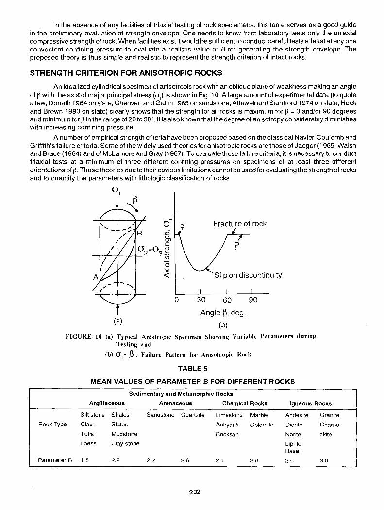
STRENGTH CRITERION FOR ANISOTROPIC ROCKS

An idealized cylindrical specimen of anisotropic rock with an oblique plane of weakhess making an angle of J-$ with the axis: of major principal stress (o,) is shown in Fig. 10. A large amount of experimental data (to quote a few, Donath 1964 on slate, Chenvert and Gatlin 1965 on sandstone, Attewell and Sandford 1974 on slate, Hoek and Brown 1980 on slate) clearly shows that the strength for all rocks is maximum for p = 0 and/or 90 degrees and minimum for~) in the range of 20 to 30°. It is also known that the degree of anisotropy considerably diminishes with increasing confining pressure.

A number of empirical strength criteria have been proposed based on the classical Navier -Coulomb and Griffith's failure criteria. Some of the widely used theories for anisotropic rocks are those of Jaeger (1969, Walsh and Brace (1964) and of Mclamore and Gray (1967). To evaluate these failure criteria, it is necessary to conduct triaxial tests at a minimum of three different confining pressures on specimens of at least three different orientations of ~i. These theories due to their obvious limitations cannot be used for evaluating the strength of rocks and to quantify the parameters with lithologic classification of rocks

o. ~

0

(a)

Fracture of rock

Slip on discontinuity

30 60

Angle~. deg.

(b)

90

FIGURE 10 (a) Typical Anistmpic Specimen Showing Variahle Parameters during Testing and

(b) 01

- ~, Failure Pattern for Anisotropic Rock

TABLE 5

MEAN VALUES OF PARAMETER B FOR DIFFERENT ROCKS

Sedimentary and Metamorphic Rocks

Argillaceous Arenaceous Chemical Rocks Igneous Rocks

Silt stone Shales Sandstone Quartzite Limestone Marble Andesite Granite

Rock Type Clays Slates Anhydrite Dolomite Diorite Charno-

Tuffs Mudstone Rocksalt No rite ckite

Loess Clay-stone Liprite Basalt

Parameter 8 1.8 2.2 2.2 2.6 2.4 2.8 2.6 3.0

232

Mean

Stal'ldard Deviation

TABLE 6

MEAN AND STANDARD DEVIATION OF BAND m PARAMETERS

FOR DIFFERENT INTACT ROCKS

Argillaceous , Arenaceous Chemical

8 m 8 m 8 m 8

2.10 4.04 2.15 5.18 2.51 5.74 2.73

0.29 3.27 0.34 4.99 0.34 4.27 0.43

Igneous

m

11.12

9:5a

Using the non-linear failure envelope predicted by Griffith's theory for plane compression and through a process of trial and error, Hoek and Brown (1980) presented an empirical failure criterion applicable for both isotropic and anisotropic rocks,

wherein

s = 1 for intact rock, and

= 0 for crushed rock,

o 1 = a3 + (mac a3 + sa~)

m =.varies widely - a function of type and quality of rock.

'h

... (8)

In order to predict the strength of anisotropic or jointed rock from the proposed criterion, Eq. 13 can be written as:

where aci = uniaxial compressive strength of rock with a weak plane or a joint oriented at~ greater than zero degrees, and

B. = material constant for the joint orientation. I

The strength predicted from Walsh and Brace, Jaeger, Hoek and Brown and also from the proposed theory at o

3=25 and 125 Kg/cm2 for Kota sandstone are presented in Fig. 11 along with the experimental results.

Both Walsh and Brace and Jaeger criteria yield poor prediction. Using the proposed criterion, the value of B. at 13=0° is 2.69 whereas at 13=30° this value is 2.51. The values of Bi for other orientations (13 = 65° and 13 = 90°) fall in between these two values indicating that the variation of B. with 13 is small, Thus one can consider B. to be a constant for a particular rock, and the prediction of strength v-!-ill be sufficiently accurate for general use~ On the other hand, for Kota sandstone using Hoek-Brown criterion, the variation in m is from 13.25 to 7. 77 and that in s is from 1 to 0.63 for different values of 13. Also for the proposed criterion, the coefficient of determination (r2

) at different orientation is above 0.999 whereas in the case of Hoek-Brown criterion, it is around 0.94 indicating an excellent matching of experimental results with the proposed criterion.

The applicability of this proposed criterion was verified (Rao, 1984) for the results of other anisotropic rocks like Green river shale, Arkansas sandstone and Per mean shale (Chenevert and Gatlin, 1965) I Martinsburg shale (Donath 1964), Texas slate, Green river shale-1 and 2 (Mclamore and Gray 1967) I Barnsly hard coal (Pomeray et a/., 1971 ), fractured sandstone (Horino and Ellickson, 1970) and Penrhyn slate (Attewell and Sandford 1974). The analysis of the data of these rocks indicates that except for Texas slate and P~nrhyn slate, the values of a for all other rocks is around 0.80. The variation between B and B. for these rocks is small, while

. . I the variation in m and m, and sands .. is large. The variation of B. with 13 is also very small when compared with the variation in m and s

1for these rocks. The predictions using these values are presented only for two rocks in

Figs. 12 and 13. Experi~ental results superimposed for comparison in these figures suggest better prediction of strength from the proposed criterion. Higher values of coefficient of determination also confirmed the versatility of the approach. Further the vcilidity of B values suggested for isotropic rocks has been confirmed for adoption even for anisotropic rocks, and thus the values of B suggested for various rock types in Table 5, for intact isotropic rocks are applicable for anisotropic rocks as well.

233

1800

1600

(\1

Exeprimental data

o cr3 = 25 kg/cm 2

• 0'3 = 12.5 kg/cm 2

Walsh & Brace criterion Jaeger single plane of weakness criterion Hoek- Brown Proposed

_5 1400 ...... , .. ~····-········-···--·· Ol

..::£ ... <J3 = kg/cm 2

~ 1200 • 25

A 50 - Proposed criterion

..c 0> c ~ 1000 1800 ·- 0 75 ---·Hoek & Brown criterion (/) X 100 Cl> .... :::J

·n; 800 u.

N

E ~

1600

600

20 60 80 ~.degrees

Cl ~

..c "5 c Cl> .... -(/)

Cl> .... :::J

FIGURE 11 Comparison hetween predicted and Measured ·n; Strengths for Kota Sandstone u.

1400

800

~.degrees

ROCK MASS STRENGTH FIGURE 12 Comparison hetween predicted and Measured

Strengths for Kota Sandstone

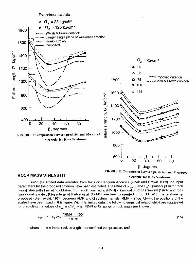
Using the limited data available from tests on Panguna Andesite (Hoek and Brown 1983) the input parameters for the proposed criterion have been estimated. The ratios of o crrfoc and BJB (subscript m for rock mass) alongwith the rating obtained from rockmass tating (RMR) classification of Bieniawski (1974) and rock mass quality index (Q-system) of Barton eta/. (1974) have been presented in Fig. 14. With the relationship proposed (Bieniawski, 1974) between RMR and Q system, namely, RMR = 9 loge 0+44, the positions of the scales have been fixed in this figure. With this limited data, the following empirical relationships are suggested for predicting the values of ocm and Bm when RMR or Q ratings of rock mass are known :

where

[RMR - 100] = a exp ----

c 18.75

ac= intact rock strength in unconfined compression, and

234

... (15)

Experimental results ---- Proposed criterion

9000 - Hoek & Brown cr 3

, kg/cm2

2812

8000 ,. 2109

7000 t(/

// "' E ~

XI

_o_ /1 ~ 1406 6000

b _/' .c -0> 5000 c

Q) X .... -(/)

Q) 703 .... ::J 4000 "(U u.

3000

2000 • (Data Mclamore & Gray 1967)

0 20 40 60 80

Ji, degrees

FIGURE 13 Comparison between Predicted and Measured Strengths for Texas Slate

0.001 0.01 0 1 10 10 100

1 ... v I• v 1.0

v r ~

/ v

0.1 ~

B or 0.01 Oan Oc

0.001 I= e Bm/B

... crcm/Cfc

0.000 1

0 10 20 30 40 50 60 70 80 90 100 I Very Poor I Poor J FU I Qood ] Very good f

CSIR GEOMECHANICS CLASSIFICATION, RMR

FIGURE 14 Plot of 0 m I Oc and B,. I B for Panguna Andesite against Rock

Mass Classification

235

um =rock mass strength in unconfined compression,

and 8 [RMR- 100] = exp• -----

75.5 ... (16)

where 8 = material constant for intact rock, and

8 = material constant for rock mass. m

By assessing the rating values of rock mass from the field, estimation of am and ucm could be conveniently made either from Eqs. 15 and 16 or from the values given in Table 7.

With these values of Bm and ocm' the strength of rock mass can be estimated by modifying Eq. 13 to the form

TABLE 7

VALUES OF B,jB FOR PANGUNA ANDESITE (oc = 2655 kg/cm2)

Ratio RMR

100 90 80 70 60 50 40 30 20 10

u ,ju c c 1.0 0.58 0.34 0.20 0.12 0.07 0.04 0.02 0.01 0.008

Bm/8 1.0 0.87 0.77 0.67 0.59 0.52 0.45 0.39 0.35 0.304

( 0'1 - 0 J)m { Ocm l a ... (17) = Bm ~~) 03

It should be noted that the relationships proposed above (Eqs. 15 and 16) for evaluation of ocm and am are based on very limited but reliable field experimental data. More field data is essential to refine these relations. However, these relations could be very well adopted for the analysis of most preliminary qesigns.

The great advantage and most significant aspect of the proposed criterion is that, based on lithologic classification, only one parameter has to be appropriately chosen from the Table 5. When no laboratory facilities exist to test intact rock specimens under a range of high confining pressures, this Table 5 and Eq 17 provide a means to arrive at the most appropriate parameters for design. When once the failure envelope is arrived at, the shear strength parameters c and <1> could be easily estimated for the appropriate stress range anticipated.

If some minimum laboratory facilities exist, at least one intact rock specimen could be tested at a convenient confinirfg pressure. Using the values of o

1 and o

3 from the test, choosing a = 0.8 and knowing nc of

the intact rock, a could be estimated and checked with the values given in Table 5, and adopted to generate the entire failure envelope. With this value of a, using Eqs. 15 and 16, o · and 8 for the rock mass could be estimated

em m

anct the strength envelope for the rock mass could be predicted. The proposed failure criterion has therefore wide application.

INFLUENCE OF A SINGLE PLANE OF WEAKNESS In a laboratory test, orientation of the plane of weakness with respectto principal stress directions remains

unaltered. Variation of the orientation of this plane can only be achieved by obtaining cores in different directions. In a field situation either in the foundations of dams, around underground or open excavations, the orientation of joint system remains stationary but the directions of principal stresses rotate resulting in a change in the strength of rock mass.

Jaeger and Cook (1979) developed a theory to predict the strength of rock containing a single plane of weakness. It assumes that the failure will take place as a consequence of sttding along the plane of weakness or a joint plane and is expressed as

2c + 2o3 tan <jJ

( 1 - tan <1> tan p ) sin 2() ... (18)

where <1> = friction angle.

Failure by sliding will occur for all values of 11 falling between <jJ and goo The minimum strength is obtained

236

when tan 2~ =-cot ljl i.e.

(o1

- oJ min = 2(c + o3

tan «j>) [(tan2 q> + 1 )"''+ tan !j>) ... (19)

This suggests that one has to first estimate the values of c and !jl along the joint plane. It is not clear whether the values of c and «j> are constant or vary with the orientation of joint plane. The test results reported by various investigators on anisotropic strength of rocks indicate only the variation of (o

1 - o

3) and not the variation of cor

!jl with~·

An experimental programme was executed (Yaji, 1984) on cylindrical specimens of plaster of Paris, red sandstone from Kota region of Rajasthan and on pink granite of Guledgudda quarries in Karnataka with different orientations of cut planes. These three materials cover a wide range of compressive strength commonly observed for weak to extremely hard intact rocks. Table 8 provides their physical and engineering properties. This study was conducted with an objective to obtain answers to the following aspects :

1. Does failure always take place by sliding along the plane of weakness ? Could it be that fracture

TABLE 8

PHYSICAL AND ENGINEERING PROPERTIES OF ROCKS USED FOR JOINT STUDIES

Material

Property/Parameter Plaster of Paris Sandstone Granite

1. Mass density (KN/m3) 12.25 22.5 26.5

2. Specific Gravity 2.61 2.63 2.69

3. Porosity (per cent) 60 12 <1

4. Uniaxial Compressive Strength o0(MN/m2) 9.5 70 123

5. Tensile Strength (MN/m2) 2.6 7.8 14.7

6. Tangent Modulus E1 (GPa) 1.0 5.1 10.8

7. Cohesion Intercept (MN/m2) 2.17 14.0 25.5

8. Angle of Friction (cW 40.5 44.0 46.5

9. Deere and Miller (1966)

Classification EL CL BL

takes place across the weak plane for some orientations?

2. How should one account for the variation of 00

, c and !jl with the orientation of weak plane?

3. How does the roughness along the joints alter the value of o0

, c and !j>?

Studies on the three materials mentioned above revealed some interesting findings which are covered under various subheads in the following;

STUDY ON PLANAR jQINTS

This study is significantly different from the previous studies conducted on joints by Patton {1966), Ladanyi and Archambault (1971), Barton {1973), Barton and Chou bey {1976) and Schneider {1976) wherein direct shear tests were carried out on joint planes and failure was by·sliding over the joint plane or by shearing of the asperities. Also the mode of failurewas influenced by the material strength and stress level.

In the present investigation specimens of Plaster of Paris were cast to have the joint plane at desired orientation using matching metal castings to obtain joint planes within the permissible limits of tolerance. For sandstone and granite, the specimens were cut along the desired inclinations and lapped to the specifications of ISRM to match the joint. Unconfined compression and triaxial tests conducted on these three materials revealed the following:

1. The modes of failure of specimens with planar joint under different confining pressures are summarised in Table 9. It is very clearly brought out that failure occurs predominetly by sliding for values of 11 ranging from about 30°- 60°. For other rang~rs of~ the failure pattern changes from vertical splitting to shearing across the joint plane, ignoring the presence of joint to propagate sliding. Splitting and slabbing are observed at lower confining pressure ranges which changed to shear failure across the .joint plane at higher o

3. Therefore, it is

237

120

100

80

6J' E ........ z 60 ~ -·c::r

b 40

20

0

Granite

crc = 0.07772P2- 6.093p + 113.6

Sandstone

crc = 0.04012P2- 3.018f +56.6

Plaster of Paris

crc = 0.005158P2- 0.3416P

0 15 30 45 60 75 90

P (degree)

+ 6.654

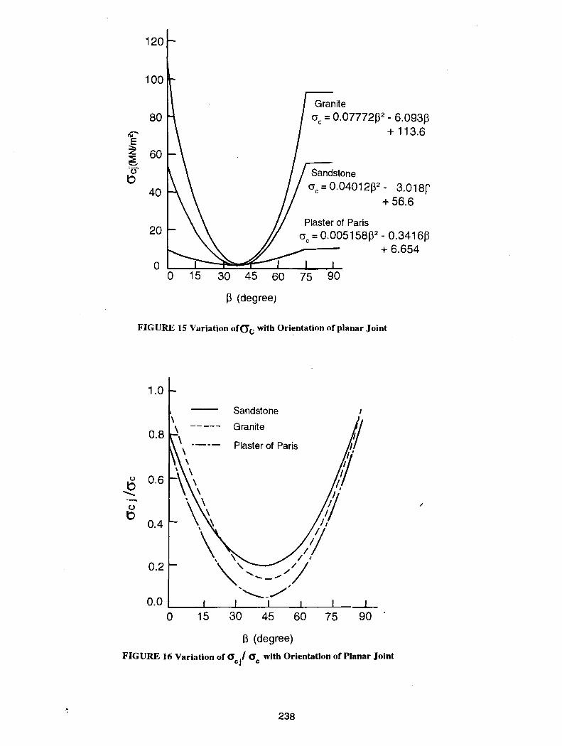
FIGURE 15 Variation ofO"c with Orientation of planar Joint

1.0

Sandstone

----- Granite 0.8

Plaster of Paris

() 0.6 b ........ 0 b

0.4

0.2

0.0 .___-~---'----L---1.---.JL....-___L_ 0 15 30 45 60 75 90 .

B (degree)

FIGURE 16 Variation ofCJc/ CJc with Orientation of Planar Joint

238

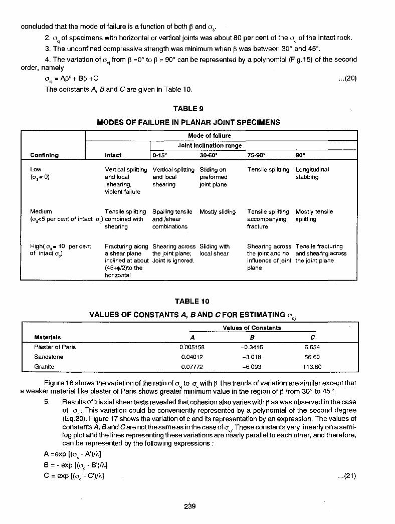
concluded that the mode of failure is a function of both p and a3

•

2. ac; of specimens with horizontal or vertical joints was about 80 per cent of the l\ of the intact rock.

3. The unconfined compressive strength was minimum when p was between 30° and 45°.

4. The variation of ac; from ~ =0° to~ = goo can be represented by a polynomial (Fig.15) of the second order, namely

ac;=A~2 +B~+C ... (20)

The constants A, Band Care given in Table 10.

TABLE9

MODES OF FAILURE IN PLANAR JOINT SPECIMENS

Mode of failure

I Joint Inclination range

Confining Intact I o-15· 30-60° 75-90° go•

Low Vertical splitting Vertical splitting Sliding on Tensile splitting Longitudinal (o3 • 0) and local and local preformed slabbing

shearing, shearing joint plane violent failure

Medium Tensile splitting Spalling tensile Mostly sliding. Tensile splitting Mostly tensile (o

3<5 per cent of intact oc) combined with and /shear accompanying splitting

shearing combinations fracture

High( o 3 • 10 per cent Fracturing along Shearing across Sliding with Shearing across Tensile fracturing of intact oc) a shear plane the joint plane; local shear the joint and no and shearing across

inclined at about Joint is ignored. influence of joint the joint plane (45+cp/2)to the plane horizontal

TABLE10

VALUES OF CONSTANTS A, BAND C FOR ESTIMATING ac1

Values of Constants

Materials A 8 c Plaster of Paris 0.'005158 -0.3416 6.654

Sandstone 0.04012 -3.018 56.60

Granite 0.07772 -6.093 113.60

Figure 16 shows the variation of the ratio of a . to a with ~ The trends of variation are similar except that CJ C

a weaker material like plaster of Paris shows greater minimum value in the region of p from 30° to 45 °.

5. Results of triaxial shear tests revealed that cohesion also varies with~ as was observed in the case of uci' This variation could be conveniently represented by a polynomial of the second degree (Eq.20). Figure 17 shows the variation of c and its representation by an expression. The values of constants A, Band Care not the same as in the case of uc. These constants vary linearly on a semi­log plot and the lines representing these variations are nkarly parallel to each other, and therefore, can be represented by the following expressions :

A =exp [(u - A')/1..] .c

B = - exp [(ac - B')/1..]

C = exp [(uc- C')/1..] ... (21)

28.0

24.0

20.0 """' "' E --z 16.0 ~

c 0 ·u;

12.0 .... Q) ..c 0 ()

8.0

4.0

0.0 0

Granite

c = 0.01751 J3 2- 1.394J3 +25.48

Sandstone

c = 0.006593J32 - 0.5198J3 +12.69

Plaster of Paris

c = 0.001 035J32 - 0.07958J3

15 30 45 60 75 90

f3 (degree)

+1.692

FIGURE 17 Variation of Cohesion with Orientation of Planar Joint

A'= 272 8' = 103

-8.0 C' = -20 A. = 37.32

-6.0

(.) -4.0 "0 c

"' CD -2.0 <i.

c: 0> 0

...J 0.0

2.0

4.0

0.0 0 20 40 60 80 100 120

O"c (MN/m2)

FIGURE 18 Variation of Cohesion Coefficlerus A.B and C will\ O'c

240

1.0

0.8

0.6

·-(.) 0.4

0.2

0

Sandstone

---- Gran~e

---- Plaster of Paris

15 30 45 60

P (degree)

75 90

FIGURE 19 Variation of cjc with Orientation of Planar Joints

The values of A', B', C' and A. are included in Fig. 18. For known values of oc of intact rock, as it appears, one could estimate the constants and evaluate the values of c afong planar joint. This study has clearly brought out that the variation of cohesion, c, along planar joints cannot be ignored. Therefore, the cohesion in Jaeger- Cook equation (Eq. 1.8) cannot be assumed to be constant. It also implies that with the rotation of principal stress directions, the cohesion along the jQint plan~ must also be considered accordingly. The variation of the ratio of cohesion of planar joint to that of the intact specimen with ~ is shown in Fig. 19. Here again the weak rock-like material suggests greater reduction in cohesion compared to stronger rocks.

6. The variation of friction angle cp with ~ for all the three materials is small. For plaster of Paris, the variation is between 39.6° to 42.4° for values of ~ =0° to goo and also for the range of confining pressures adopted. In the case of sandstone, these values of cp fall between 42.4° and 45.5°, and for granite between 40.5 o and 46.5 o. As such, the variation in the values of cp for the three materials having distinct unconfined compressive strengths is indeed small. Therefore, the values of cp to be adopted with rotation of principal stress directions could be considered to be constant over the range of~·

STUDY ON ROUGH JOINTS

More than 30 different types of step-shaped and berm-shaped joints were produced in cylindrical specimens of plaster of Paris, with varying number of steps or berms along the length of different inclinations of ~· These specimens were tested in unconfined compression and triaxial states. Some of the interesting findings are summarized below :

1 . Roughness produces interlocking effect along the joint planes. Greater the roughness greater is the interlocking effect. Consequently, longitudinal spilitting at lower confining pressures and clear well defined shear failure across the joint plane were observed.

2. Increase of roughness results in higher oci approaching the strength of intact specimen.

3. Figure 20 for different roughflesses produced along the joint planes inclined at p = 45° or 60° suggests thatthe ratio of cohesion of joint specimen (c~ to that of intact specimen (c) increases with roughness. The roughness is defined as the ratio of amplitude of the protrusion on the joint surface to the joint length. When the roughness is almost equal to zero, this ratio of cohesion values also

241

(.) -(.)

1.0

0.8

0.6

0.4

0.2

0.0 0.20

~

0.25 0.30 0.35

Jd/L

0.40

1.8

1.6

1.4

1.2

1.0

0.8 0.45 0.50

6" E z ~ -(.)

FIGURE 20 Variation of Coht:sion with Amplitude of Protrusion for Stepped Shaped Joint ( ~ = 600)

becomes nearly zero as suggested by tests on planar joints in plaster of Paris for similar values of p.

4. The value of friction angle did not change irrespective of the type of rough joints and its inclination and was close to that of an intact and a planar joint specimen.

5. Contrary to what has been observed in the case of planar joints rough joints indicate increase of c1c up to a maximum value of 0.72 when 13 = 45°, due to the high degree of interlocking. A similar trend of higher values of o c· at 13 = 45° was also observed. From Mohr -Coulomb criterion, the uniaxial compressive strength oc ~f intact rock can be expressed as

2 c coscp de =

1 - sincp

. oc = 2 coscp I. e.

c 1 - sincp

... (22)

Most rocks which are coarse grained, massiv~, crystalline or arenaceous and having similar values of friction angle will have similar ojc ratios. For all the three materials, cp varies from 40.5° to 46.5°, the ratio ojc varies from 4.4 to 5.0. For most rocks when <1> varies from 25 to 45°, this ratio may range from 3 to 5. One very interesting observation from the study of various joints of these three materials is that the values of ratio ojc or oc/c

1 essentially lie between 4 and 5. Planar join!s exhibited lower ratios.

From the above findings it is obvious that whenever rotation of principal stress directions takes place, the following may be expected :

(i) The corresponding changes in oc and c may have to be appropriately considered;

(ii) Further, whenever first order protrusions· on the joint planes do not interfere i.e. the gouge material is thick enough, one would expect considerable reduction in c with the rotation of principal stresses as was observed in the case of planar joints;

(iii) If the protrusions on the joint plane interfere and produce inter-locking as is the case often with

242

1.0

0.8

crcR 0.6 or

ER

0.4

0.2

0.() 0

ere= 11.32 MN/m2

cr1 = 1.95 MN/m2

CTCR=CTCj/CTc EA = Ej I E

20 40 60

No. of Joints I m, i. 80 100

3.0

2.4

E I

-E- 1.8

or

cr~;i crr 1.2

0.0

Ej

~1 .ttiJoi dj = DVB

Dj = Depth of joint from loading face

B = Width of loaded area

intact-

O"c j la-c= 0.42 dj + 0.5

0.4 0.8 1.2 1.6 2.0

dj

l'll;tJRE 21 Variation or Strength and Modulus and Joint Frequency ror Plaster or Paris FIGURE 22 V•rialion or Sire .... IIDII Modulus with Loc:alloa

or Slnxle Joint (Jl • 0) ror Plaster or Paris

closed joints, the variation in c with the rotation of principai stresses may not be significant for con­sideration;

(iv) Even the values of Modulus number, K, and modulus exponent n, of Janbu's (1965) expression relating initial tangent modulus (E;) with confining pressure cr

3 also undergo considerable change

with the rotation of principal stresses;

(v) The value of K attains a minimum and the value of n attains a maximum in planar joints for f3 = 45° The variation in K is similar to that of c in planar joints.

(vi) The variation of friction angle with the rotation of principal stresses may not be significant, more so, with rough joints.

INFLUENCE OF NUMBER AND LOCATION OF JOINTS

For plaster of Paris representing weak rock, the variation of number of horizontal joints per meter length (Jn jointfrequency) with the ratio of uniaxial strengths of joint and intact specimens under unconfined compression has been presented in Fig. 21 . The ratio of moduli of jointed specimen to that of the intact specimen is also included in this figure. The reduction of strength is observed to be lower than the modulus values with jointfrequency. When there are 10 joints/m, the reduction in strength is only 10 per cent. whereas for 100 joints/m, the corresponding reduction is 50 percent. On the other hand, the reduction in modulus is about 70 per cent for 100 joints/m.

The location of a single joint with respect to the loading surface defined by d1 = D/B (ratio of depth of joint

Di, to the width or diameter, 8, of the loaded area) greatly influences the strength of rock, Fig. 22. When the joint is located very close to the loading face, the strength of jointed rock is about 50 per cent of the intact value. Its effect is as important as the presence of 1 00 joints/m uniformly spaced. With the location of the joint away from the loading face, the strength of joint rock increases and attains a value, same as that of the intact rock when the joint is located at about 1 .2 B or beyond below the loading face. The ratio of moduli of joint to intact specimens with the variation of the location of joint is also shown in the Fig. 22. The modulus of the joint rock is higher than that of the intact rock so long as the joint is within the depth equal to the width of the loaded areas. In fact, the stiffness of the rock is highest when the joint is close to the loading face contrary to what has been observed for strength. Influence ofthe location of a joint on the stiffness continues to decrease even upto a depth twice the width of the loaded area.

243

0 0

.><

~ D

t:)

0

~ c: -~ u

::::> "0 \!) ..... .c ~ c: ~

r:;>

80

70

60

50

4G

30

20

10

0 5 10 15 20 25

Cfc/cr3 30 35

FIGURE 23 Variation of Anisotropy with the Ratio O'c; / (j 3

• Martinsburg slate (Donath 1972)

• Fractured S. St. (Horino and Eilickson 1970)

0 Texas slate (McLamore and Gray 1967)

+ Barnsly Hard coal (Pomeroy et al. 1970)

)( Green River shale (Chenevert and Gatlin 1965)

• Green River shale - I ( Mclamore and Gray 1967 )

D. Green River shale - II ( Mclamore and Gray 1967 )

D Arkansas s. st. (Chenevert and Gatlin 1965)

s. st. = Sandstone

40 45

Investigations are in progress to know how far this behaviour is also observed in different rocks. The influence of orientation, number of joints and the effect of confinement on the response of different rocks are being studied.

From Fig. 23, one also notes thatthe influence of anisotropy fast deteriorates for values of uju3

1ess than 5. When aja

3 = 1, in most weak rocks, it appears that only about 10 per cent of strength anisotropy may be

observed. For practical purposes one may assume that the effect of-anisotropy may not be significant when the insitu hydrostatic stress Is the same as the unconfined compressive strength of intact rock in the case of well defined joint rock mass.

MODULUS OF ROCK MASS

Bieniawski (1978), based on the data collected from field tests, suggested an empirical relation for the estimation of modulus of elasticity (£,j of the rock ma!Ss (in GPa) as

Em = 2 RMR - 1 00 ... (23)

This equation suggests that when RMR value is 50, the modulus of rock mass is almost negligible. Even loose soils exhibit values of modulus greater than zero. Test results of Yaji (1984) on smooth and rough joint planes and the data provided in Fig. 21 on the reduction of modulus with number of joints one would expect Em/ E to be greater than zero, (where Em= modulus of rock mass and E =modulus of intact rock, both the values are in unconfined state). If the joint inclinations are essentially falling between 30° to 45° (with the vertical or major principal stress) Ej£ may be close to zero. But when the joint inclinations are nearly horizontal, ErniE could as well be equal to about 0.2. This is suggested by some field results reported by Bieniawski. Therefore, one may suggest-the following relationships for practical use :

(i) For predominantly horizontal joints

Ej E = exp (0.0217 RMR - 2.17) ... (24)

244

(ii) For predominantly inclined joints, inclined at 30° to 45° to vertical

EjE = exp (0.0564 RMR- 5.64)

STABILITY OF ROCK SLOPES

... (25)

Stability of sloping ground has attracted considerable attention of geotechnical engineers during the past few decades due to the importance of controlling and preventing landslides, design and construction of road and railway embankments and cuttings, earth and rockfill dams, open excavations for foundations of dams and open pit mines. Cuts made for roads and railways are sometimes difficult and perpetually problematic. The cost of solving the slo~ problem connected with mining can be of great economic consideration. A few million tons of extra waste would have to be mined as a result of an average slope being reduced by 3 to 5 degrees in an open pit of about 400 x 400 x 150m deep. Unlike soil slopes, rock slope stability is essentially governed by the joint sets, their relative orientation, the gouge material present in the joints and on the extent of excavation with respect to joint spacing. The mode of failure is primarily controlled by them.

MODES OF FAILURE

The modes of failure of rock mass are either circular, planar, wedge or toppling types, (Hoek and Bray 1977).

(i) Circular mode: When the sterographic representation of the joints by pi diagram does not indicate any well defined planes of orientation one would expect rotational· failure of rock mass along a curved surface; more often along a circular surface and mass movement takes place into the excavation. Such failures are expected in heavily fractured rock mass, more so when the joint material is clayey or when the joint faces are decomposed and also in coal tips and rockfills.

(ii) Planar mode :When a joint set is highly ordered, represented by a single pole concentration, the mode of failure is planar with the mass moving into the excavation, when the face of excavation is same or inclined to the strike direction of the joint plane. If the face of excavations is in the dip direction, failure by sliding along the joint plane will not result.

(iii) Wedge mode :When two or more pole concentrations are exhibited representing intersecting planes, wedge failure is likely to take place with the translatory movement of the rock mass in the form of a tetrahedron when the line of intersection of the planes of sliding daylights into the excavation.

(iv) Toppling mode :When the pole concentration lies on the opposite side of the pole of the face of excavation, failure by toppling of blocks of rock may take place particularly in steeply dipping column and sheet like rock mass structures.

Some of the rock slopes could remain almost at 45°for heights upto 200m (Hoek, 1970), essentially due to high degree of interlocking and roughness along the joint planes. More often, rock slopes have been found to be flatter than 45° when the degree of interlocking is low and the material along the joints has weathered.

Analysis of rotational type of failure of soil and rock slopes along circular or curved surface has drawn considerable attention over the years.

ROTATIONAL APPROACH

Even though the earliest work on stability analysis was carried out by Coulomb (1773) and Collin (1846), significant contributions were largely due to the classical methods developed by Swedish engineers during the period 1915 to 1925. Swedish slip-circle method of slices for rotational slides developed by Fellenius (1927, 1936) has been the most widely used conventional technique for numerous practical problems. Among other significant contributions in this area are the works of Taylor (1948), Sokolovsky (1960), Janbu (1954), Bishop (1955), Morgenstern ~nd Price (1965), Chugaev (1966) and Spencer (1967, 1968, 1969).

Bisho 's (1955) slip circle analysis formed the basis for further research in the stability analysis of slopes. This method is igorous in its content satisfying both force and moment equilibrium conditions and also considered the presence or inter-slice forces. To circumvent the rather lengthy and involved tedious numerical computations Bishop simplifird the original expression by assuming the direction of the interslice forces to be horizontal. The minimum factor of safety obtained by this method is a close approximation to the final value obtained by using the rigorous method. This implied that the factor of safety is insensitive to the distribution of internal forces. This analysis did not justify why an expression to obtain factor of safety not satisfying one of the basic conditions of

245

equilibrium should yield a solution close to the critical equilibrium state.

Morgenstern and Price (1965) suggested a method of analysing a slope using a general slip surface satisfying both force and moment equilibrium conditions and could consider slope sections with varying shear strength parameters and pore pressures. The analysis is based on the principles of limit equilibrium and need a priori assumption of the shape of the potential sliding mass as well as the distribution of internal forces. This method and the slip-circle method of Bishop gave similar values of factor suggesting insensitiveness of the factor to the varying distributions of internal forces within the potential sliding mass.

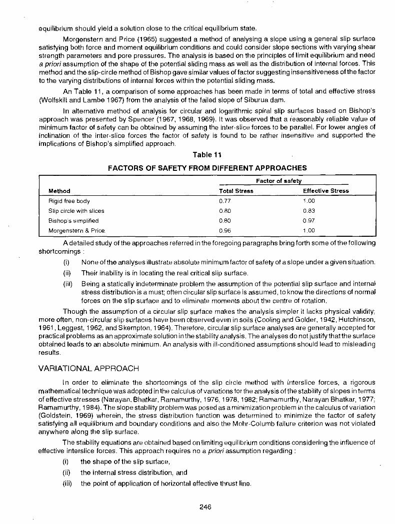
An Table 11, a comparison of some approaches has been made in terms of total and effective stress (Wolfskill and Lambe 1967) from the analysis of the failed slope of Siburua dam.

In alternative method of analysis for circular and logarithmic spiral slip surfaces based on Bishop's approach was presented by Spencer (1967, 1968, 1969). It was observed that a reasonably reliable value of minimum factor of safety can be obtained by assuming the inter-slice forces to be parallel. For lower angles of inclination of the inter-slice forces the factor of safety is found to be rather insensitive and supported the implications of Bishop's simplified approach.

Table 11

FACTORS OF SAFETY FROM DIFFERENT APPROACHES

Method

Rigid free body

Slip circle with slices

Bishop's simplified

Morgenstern & Price.

Total Stress

0.77

0.80

0.80

0.96

Factor of safety

Effective Stress

1.00

0.83

0.97

1.00

A detailed study of the approaches referred in the foregoing paragraphs bring forth some of the following shortcomings :

(i) None of the analyses illustrate absolute minimum factor of safety of a slope under a given situation.

(ii) Their inability is in locating the real critical slip surface.

(iii) Being a statically indeterminate problem the assumption of the potential slip surface and internal stress distribution is a must; often circular slip surface is assumed, to know the directions of normal forces on the slip surface and to eliminate moments about the centre of rotation.

Though the assumption of a circular slip surface makes the analysis simpler it lacks physical validity; more often, non-circular slip surfaces have been observed even in soils (Cooling and Golder, 1942, Hutchinson, 1961, Leggest, 1962, and Skempton, 1964). Therefore, circular slip surface analyses are generally accepted for practical problems as an approximate solution in the stability analysis. The analyses do notjustifythatthe surface obtained leads to an absolute minimum. An analysis with ill-conditioned assumptions should lead to misleading results.

VARIATIONAL APPROACH

In order to eliminate the shortcomings of the slip circle method with inters lice forces, a rigorous mathematical technique was adopted in the calculus of variations for the analysis of the stability of slopes in terms of effective stresses (Narayan, Bhatkar, Ramamurthy, 1976, 1978, 1982; Ramamurthy, Narayan Bhatkar, 1977; Ramamurthy, 1984). The slope stability problem was posed as a minimization problem in the calculus of variation (Goldstein, 1969) wherein, the stress distribution function was determined to minimize the factor of safety satisfying all equilibrium and boundary conditions and also the Mohr-Columb failure criterion was not violated anywhere along the slip surface.

The stability equations are obtained based on limiting equilibrium conditions considering the influence of effective interslice forces. This approach requires no a priori assumption regarding:

(i) the shape of the slip surface,

(ii) the internal stress distribution, and

(iii) the point of application of horizontal effective thrust line.

246

Two methods have been developed for obtaining the solution by this approach, namely,

(i) Indirect method (non-local variation)

(ii) Direct method (Raleigh-Ritz technique).

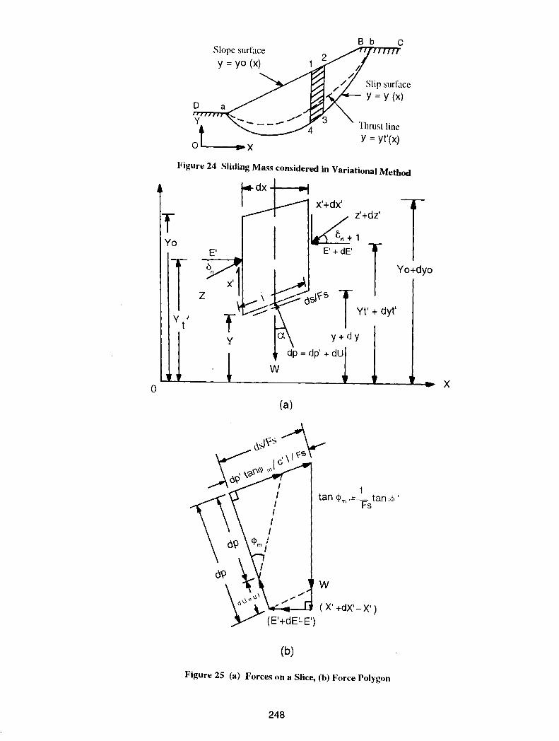
By adopting the limit equilibrium method of analysis, the stability equations of any slope in general are obtained by considering the critical state of equilibrium of the various forces acting over an infinitesimal slice situated within the potential sliding mass. Figure 24 shows a section through a slope with a general slip surface and a and b as the boundaries defined by a (X

8, y) and b (xb, y J on the slope section. The given slope is

represented by any known function y = Yo (x), i.e. DaBC in the figure and the potenti a1 sliding surface by y = y (x) with a and bas its boundary points on the slope. Functions y = Y, (x) andy= y,' (x) define the line of action of total and effective horizontal thrust lines respectively. The elemental sliding surface is represented by 1234. Figure 25 shows the various forces acting on the elemental slice and the force polygon of these forces.

The sitability equations framed under the limit equilibrium conditions (Ramamurthy, Narayan and Bhatkar, 1977) reduce to minimization problem in the calculus of variations. The problem is to find a critical slip surface yJJ(x) and shear mobilizing factor function f 0 (x) which minimizes an appropriately defined factor of safety.

The overall factor of safety (Fs) along the slip surface and average factor of safety (Fv) along the inters lice boundary were written as :

F = s

x,

J[ a1 (1 + y'~) + aJ ( a2 (Yo- Y1) (1 - h) - Y1' [y2 {Yo' - Y1' -x.

{ h' (Yo - Y1 )2 + 2h(yo - Y1 )

2 + 2h (Yo - Y1) (Yo' - Y1 1

) }

+ y 2 , { a2 ( yo - y 1 ) - i a2 aJ h ( yo - y 1 ) 2 _} ] ) ] dx

xb

[ [ a2 (Yo - Y 1 ) Y 1 ' ( 1 - h) + ;v [ ( 1 + aJ Y 2 ) { a1 (Yo ' - Y 1 ' ) -. (h' (Yo- Y1)

2 + 2h(Yo- Y1) (Yo'-- Y1'))}

+ Y2' { a1 (Yo- Y1)- ~ a2aJh (Yo- Y1)2

} aJ J Y1' ]dx

[ [ (a, (.y 0 - y,) - ~ a, a, h (y 0 - y, )' ) ( 1 + a, y, ) ) ] d>

xb

[ [ ( a1 ( yo - y 1 ) - ~ a2 aJ h ( yo - y 1 ) 2 ) ( y 1 ' - y 2 ) ] dx

Where

a, = c', a2 = y, ~=tan <j>', h(x) = ru, h'(x) = r'u•

Y,(x) = y(x), y',(x) = y'(x), Y/X) = f(x) and

y'2(x) = f'(x)

247

... {26)

... (27)

0

Slope surface

y =yo (x)

Thrust line y = yt'(x)

Figure 24 Sliding Mass considered in Variational Method

T Yo

T y J

t

E'

z

y

w

x'+dx' z'+dz'

~~ E' +dE'

~ Yo+dyo

T Yt' + dyt'

y+dy

dp = dp' + dU

(a)

1 tan <1> ,.:::_tan ,G>'

"' Fs

(b)

Figure 25 (a) Forces on a Slice, (b) Force Polygon

248

X

4:1 0.12

3: 1 2: 1 1.5: 1

ru = 0.0

0.10 q>m

0.08

c 0.06 F s y H

0.04

0.02

0.00 0 4 8 20 24 28 32 36

Slope angle (degrees), i. Figure 26 Slope Stahility Chart for Y. = 0

0.12 4:1 3: 1 2.' 1.5: 1

ru = 0.20

0.10 12 °

0.08 16° 18°

c 0.06 24 °

F • yH 0.04 28 °

30°

340

0.02 360 380 40°

0.00 0 4 8 12 16 20 24 28 32 36

Slope angle (degrees), i.

FIGURE 27 Slope Stability Chart for Y. == 0.2

c F • yH

0.00 L.._--L_.4.......1~~::....C..~l::::.oo::::.d~Q::::::~:I:....L.__J 0 4 8 12 16 20 24 28 32 36

Slope angle (degrees), i FIGURE 28 Slope Stability Chart for Y.· : 0.3

249

The minimization of the functional of the form J (y) given by Eq. 26 can be obtained by using either indirect method or direct method in the calculus of variation. The indirect method was described in detail by Narayan, Bhatkar and Ramamurthy (1976) The direct method (Ramamurthy, Narayan and Bhatakar, 1977) is very briefly presented herein for completeness and used to develop slope stability charts.

DIRECT METHOD OF MINIMIZATION

Using the well known Raleigh-Ritz technique (Gelfand and Fomin, 1963), the overall factor of safety has been minimized. The method of local variations (Chernovs'ko 1965) could also be adopted. In Ritz method the functional J [y, y

2] defining F. (Eq. 26) was not considered along arbitrary admissible functions y, (x) and Y2 (x)

but along all possible linear combinations. m

y1 (x) = ~a; l/' i (x) 1=1 ... (28) . n

y2 (x) = ~ bi l/j (x) ... (29)

where ~ and bi are unknown functions and lJ!; and ljJ are the prescribed functions of the independent variable x. The functions 'Ji; and 'Jii are referred to as basis or ihterpolation functions. The interpolation functions chosen so as to satisfy the given boundary conditions.

. .. (30)

and

... (31)

identically,

Substituting Eqs. 28 and 29 in Eq. 26, the functional J [y,, y2

] becomes a fu~ction F (~. b) of (n+m) unknown constants. The problem of minimizing F (a, b) with respect to a and b is essentially a mathematical programming problem. The coefficients (aa;• bai) are'd~termined from the'followi

1ng equation:

elf = 0 and elf = 0 t( alo el b ol. . .. (32)

Equation 32 results in (n+m) simultaneous algebric equations, solutions of which yield aa and ba The minimizing functions yo, and ya

2 are obtained from the·following expressions :

m

y~ (x) = ~ a~ ljJi (x) 1=1 ... (33)

n

y~ (x) = ~ bj lj!i (x) ... (34) j=1

Considering a homogeneous slope section and representing the surface of slope and slip surface by fourth degree polynomials and using the above referred equation, numerical results were used to develop stability charts one each for ru = 0, 0.2, 0.3 and 0.4 and presented fn Figs. 26 to 29. From the rigorous indirect method it was observed that the slip surface could be represented by a fourth degree polynomial without sacrificing overall absolute minimum factor of safety. These charts are convenient to ascertain the stability of slopes when the material and slope geometry parameters are known.

The results obtained by the variational method showed variation from those obtained by Spencer (1967). Table 12 shows comparison of factors of safety for a typical case both from direct and indirect methods with that obtained by the procedure suggested by Spencer with the following properties:

250

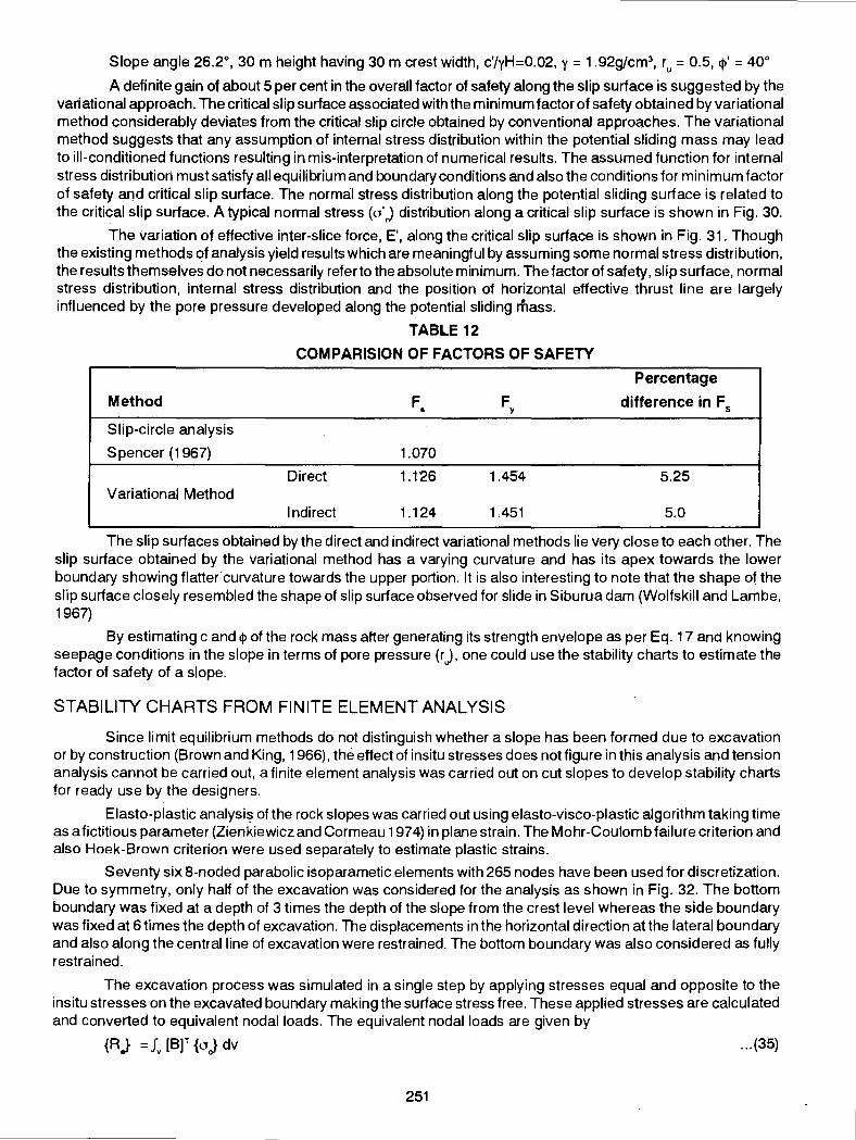
Slope angle 26.2°, 30m height having 30m crest width, c'/yH=0.02, y = 1.92g/cm3, ru = 0.5, <j>' = 40°

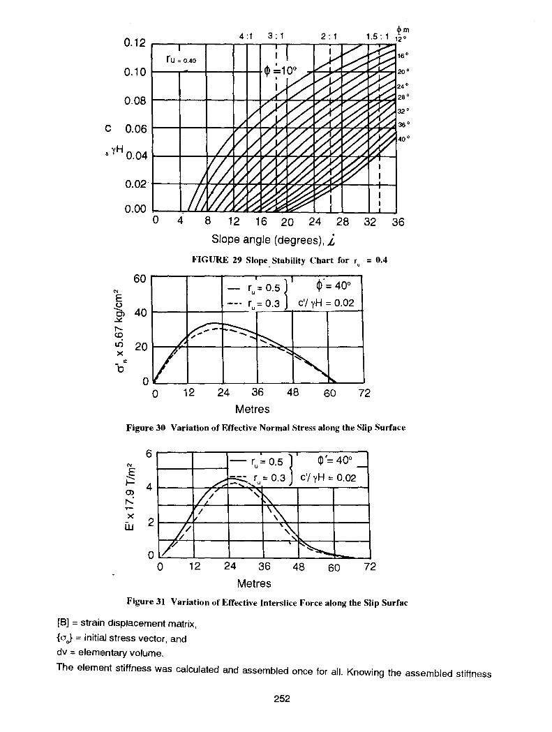
A definite gain of about 5 per cent in the overall factor of safety along the slip surface is suggested by the variational approach. The critical slip surface associated with the minimum factor of safety obtained by variational method considerably deviates from the critical slip circle obtained by conventional approaches. The variational method suggests that any assumption of internal stress distribution within the potential sliding mass may lead to ill-conditioned functions resulting in mis-interpretation of numerical results. The assumed function for internal stress distribution must satisfy all equilibrium and boundary conditions and also the conditions for minimum factor of safety and critical slip surface. The norma] stress distribution along the potential sliding surface is related to the critical slip surface. A typical normal stress (u',) distribution along a critical slip surface is shown in Fig. 30.

The Variation of effective inter-slice force, E', along the critical slip surface is shown in Fig. 31. Though the existing methods of analysis yield results which are meaningful by assuming some normal stress distribution, the results thems-elves do not necessarily refer to the absolute minimum. The factor of safety, slip surface, normal stress distribution, internal stress distribution and the position of horizontal effective thrust line are largely influenced by the pore pressure developed along the potential sliding mass.

TABLE 12

COMPARISION OF FACTORS OF SAFETY

Percentage

Method F F difference in F 5 • y

Slip-circle analysis

Spencer (1967) 1.070

Direct 1.126 1.454 5.25 Variational Method

Indirect 1.124 1 ;451 5.0

The slip surfaces obtained by the direct and indirect variational methods lie very close to each other. The slip surface obtained by the variational method has a varying curvature and has its apex towards the lower boundary showing flatter" curvature towards the upper portion. It is also interesting to note that the shape ot the slip surface closely resembled the shape of slip surface observed for slide in Siburua dam (Wolfskill and Lambe, 1967)

By estimating c and <1> of the rock mass after generating its strength envelope as per Eq. 17 and knowing seepage conditions in the slope in terms of pore pressure (r.), one could use the stability charts to estimate the factor of safety of a slope.

STABILITY CHARTS FROM FINITE ELEMENT ANALYSIS

Since limit equilibrium methods do not distinguish whether a slope has been formed due to excavation or by construction (Brown and King, 1966), the effect of in situ stresses does not figure in this analysis and tension analysis cannot be carried out, a finite element analysis was carried out on cut slopes to develop stability charts for ready use by the designers.

Elasto-plastic analysis of the rock slopes was carried out using elasto-visco-plastic algorithm taking time as a fictitious parameter (Zienkiewicz and Cormeau 1974) in plane strain. The Mohr-Coulomb failure criterion and also Hoek-Brown criterion were used separately to estimate plastic strains.

Seventy six 8-noded parabolic isoparametic elements with 265 nodes have been used for discretization. Due to symmetry, only half of the excavation was considered for the analysis as shown in Fig. 32. The bottom boundary was fixed at a depth of 3 times the depth of the slope from the crest level whereas the side boundary was fixed at 6 times the depth of excavation. The displacements in the horizontal direction at the lateral boundary and also along the central line of excavation were restrained. The bottom boundary was also considered as fully restrained.

The excavation process was simulated in a single step by applying stresses equal and opposite to the insitu stresses on the excavated boundary making the surface stress free. These applied stresses are calculated and converted to equivalent nodal loads. The equivalent nodal loads are given by

{Rj = fv (B]T {oJ dv ... (35)

251

0.12 4 :1 3: 1 2: 1

ru = 0.40

0. 1 0 1---......... .....__-+---+-+--t

c 0. 06 l---+--+---b£1174"7'47'f-::.~V:~~~7"7":1

s yH 0.04 1-~-+H~~l,L:,~~Nm¥7?1~---1

0 4 8 12 16 20 24 28 32 36

Slope angle (degrees), i FIGURE 29 Slope_ Stability Chart for ru = 0.4

60 - r = 0.51 $'= 40o

E --- r: = 0.3 c'/ yH = 0.02 ~ 40 1------lf-----t-- '~-~r---.:.-.-----t ..Y!

1'-­<.0

1.() 201--~~----~-----+-~~---+------1 X

OL--~-~--L-~--~~ 0 12 24 36 48 60 72

Metres

Figure 30 Variation of Effective Normal Stress along the Slip Surface

6 - r,~ 0.5 r ~·= 40'-

~ ~,.! = 0.3 c'/ yH = 0.02 u

"' E ;:::: 0> 4 ,...... L!' '~

~ X

[u 2 I I \~

lt

J/ '~

...-

0 1// ~~ 0 12 24 36 48 60 72

Metres

Figure 31 Variation of Effective Interslice Force along the Slip Surfac

[8] =strain displacement matrix,

{oJ = initial stress vector, and

dv = elementary volume.

The element stiffness was calculated and assembled once for all. Knowing the assembled stiffness

252

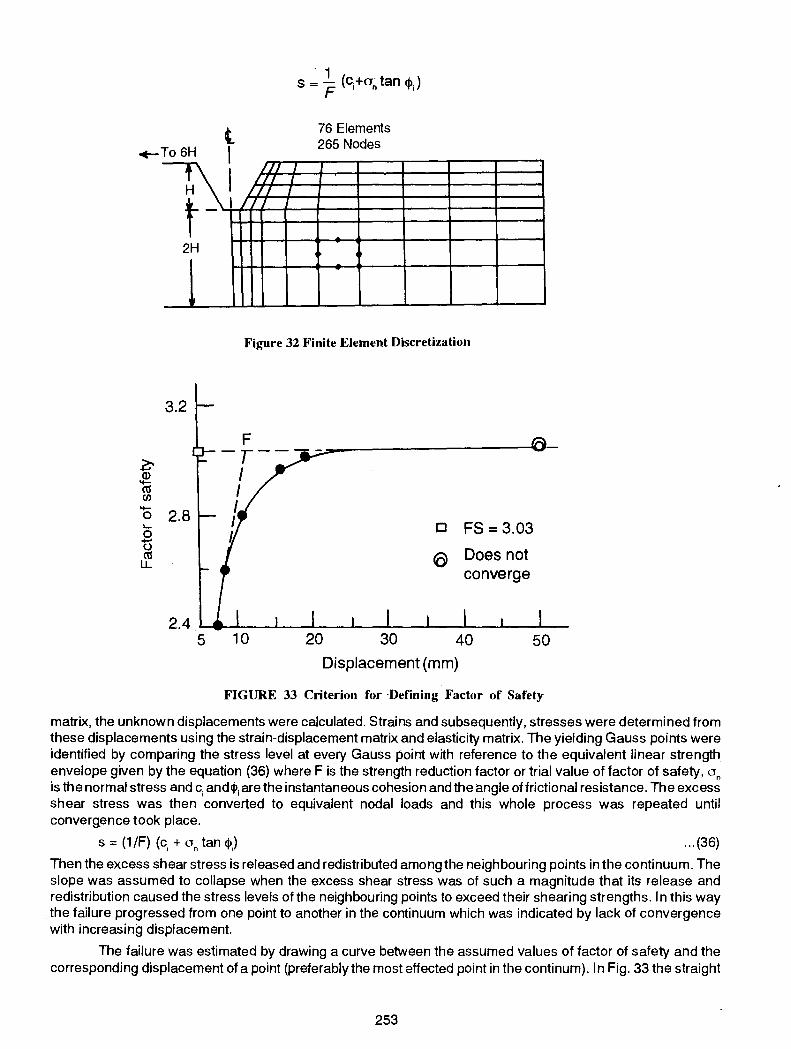
+-To 6H

H

t-2H

>--Q) -cu (/) - 2.8 0 ,_ 0 -() cu LL

t I I I

I_Lf 1 /II I

I I I I I

76 Elements 265 Nodes

Figure 32 Finite Element Discretization

[J FS = 3.03

6 Does not converge

Displacement (mm)

FIGURE 33 Criterion for ·Defining Factor of Safety

matrix, the unknown displacements were calculated. Strains and subsequently, stresses were determined from these displacements using the strain-displacement matrix and elasticity matrix. The yielding Gauss points were identified by comparing the stress level at every Gauss point with reference to the equivalent linear strength envelope given by the equation (36) where F is the strength reduction factor or trial value of factor of safety, un is the normal stress and ci andcjli are the instantaneous cohesion and the angle of frictional resistance. The excess shear stress was then converted to equivalent nodal loads and this whole process was repeated until convergence took place.

s = (1/F) (c, +on tan cj>) ... (36)

Then the excess shear stress is released and redistributed among the neighbouring points in the continuum. The slope was assumed to collapse when the excess shear stress was of such a magnitude that its release and redistribution caused the stress levels of the neighbouring points to exceed their shearing strengths. In this way the failure progressed from one point to another in the continuum which was indicated by lack of convergence with increasing displacement.

The failure was estimated by drawing a curve between the assumed values of factor of safety and the corresponding displacement of a point (preferably the most effected point in the continum). In Fig. 33 the straight

253

a = 7oo H = 40m

'A.'cq, = 0.06

Trial factors of safety

----- 1.00

1.10

1.15

1.20

Figure 34 Development of Yielding Zone with Factor of Safety

line portions of the curve are extended to give point F which decided the factor of safety. A typical development of yielding zones with increase of trial factor of safety is shown in Fig. 34.

For developing stability charts for ready use by the designer, a parametric study was carried out. It was observed that :

(i) the Young's modulus (E) affects only the magnitude of the displacements and not the factor of safety;

(ii) the Poisson's ratio (u) within the range of 0.15 to 0.35 did not influence the factor of safety; and

(iii) the effect of stress ratio (K) was insignificant on factor of safety.

The combined effect of c, y, Hand cp was considered by introducing a non-dimensional factor A.cq> = yH tan cp/c (Janbu, 1954). It was observed that nearly same values of A.ccp were obtained for the same factor of safety and same slope angle. Similarly stability number (Taylor, 1948) Sn=(c/FyH), was determined. Figure 35 shows the relationship between S" and 1 /A.ccp (using finite element method) for different values of slope angle, i, (Sharma, Ramamurthy and Ailawadi, 1984). In this figure the stability number as per Hoek-Bray charts (1977) are also included. The stability numbers as per limit equilibrium method (LEM) obtained by Hoek-Bray charts are higher than from the finite element method (FEM) suggesting underestimation of factor of safety by the former method. For a 90° rock slope, Hoek-Bray charts underestimate factor of safety by about 38 per cent. As the slope angle of cut slopes in rock decreases, the difference in factors of safety from both the approaches decreases. A better appreciation of the comparison of factors of safety obtained by Hoek-Bary charts and finite element approacch can be made from Fig. 36.

Using m and s parameters of Hoek-Brown criterion on a similar basis as shown on the foregoing for finite element analysis, stability e;hart for a dry/drained cut rock slope has been developed (Ramamurthy, Sharma and Ailawadi 1985, Ailawadi 1985). Non-dimensional parameters ·

A,ns as = _.s.__

'YHm and stability number, S'" =

254

0.28

0.24

/ 0 /

c§l 9f

\ol I

LEM --FEM

II 60 o

cE 0.16 t--+--t---:-:~T-7-:::::=t-~:;j:::::::::=t===1==--..... Q) .0

§ 0.12 1--14-#~~:::::....----=lr--::::~-+--==F==~= z ~ :0 ro 8~~~~~--~~~~~----~====;===---t---10° U5 0.0

8

-- 6 :::2: LU u. >. -Q) -(\1 ({) -0 ..... 0 -() (\1 u.

4

2

0 0

------10° ----

0.2 0.4 0.6 0.8 1.0 1.2

Non- dimensional factor(C/yH tan~)

FIGURE 35 Combined Stability Chart by LEM and FEM

. ·~ - goo

6.(, 70°

.{, 45°

2 4 6 8

Factor of safety (Hoek & Bray)

1.4

FIGURE 36 Comparison of factors of Safety from FEM and Hoek-Bray Method (1977)

255

0.8

i. = goo

~

;, ~ 0.4 t--:-::~--t--t-t-r-~~Y..--t::::=~:t:-r-1/ lL

_ c I (J) ' ~

0.001 0.01 0.1

0 s Ams + -­

rHm

1.0

FIGURE 37 Slope Stahility Chart by LEM and FEM using m and s Values

LEM I= EM

10.0

have been developed to form the stability chart linked through slope angle, i, Fig 37. For limit equilibrium approach adopting Bishop's simplified method (1955) similar stabiiity chart was developed and superimposed on that obtained from the finite element method in Fig.37. This figure provides a ready comparison of limit equilibrium and finite element methods. The limit equilibrium method may either underestimate or overestimate depending upon the slope angle and A.ms value. For a 90° slope with A.ms = 0.001, the limit equilibrium method underestimates the factor of safety by as much as 50 per ent. For a slope of 45° and A.ms = 0.001, this method overestimates the factor of safety by 41 per cent when compared to that given by finite element method. For cases with the combination of i and A.ms' both the methods suggest similar factors of safety.

A designer will find it quite convenient to use these charts to try various alternatives by choosing any of the methods of analyses i.e. finite element or limit equilibrium method adopting any failure criterion developed either from Mohr-Coulomb (Eq.17) or Griffith (Eq 8) approaches i.e. either using c and q> or m and s parameters of rock mass.

The primary objective of preparing Figs. 26 to 29, and 35 and 37 was to bring the rigorous and extensively computer oriented analyses within the reach of the designer.

STABILITY OF SQUEEZING GROUND

For the design of support system for tunnels in rock mass, estimation of rock pressures on the supports for any allowed deformation of both the rock mass and the supports is an important consideration for the stability of the tunnel. More often, the magnitude of rock load is estimated based on the qualitative description of the rock mass (Terzaghi, 1946). In suh cases deformations produced on the tunnel walls do not figure. Such an analysis to predict rock loads is empirical, soiely based on experience gained from the study of designs and some of their failures under specific conditions. This approach in course of time lead to the development of rock mass classification to aid estimation of rock loads.

ROCK MASS CLASSIFICATIONS

The most popular rock mass classifications for the estimation of rock loads are :

(i) Terzaghi's approach (1946), extensively used in India and the USA with steel support system,

(ii) Lauffer's (1958) cencept of stand up time, emerging from Stini's work (1950),

256

(iii) Deere's (1964) classification introducing rock quality index (RQD) to borelog data and incorporat­ing as such in the classifications developed later on,

(iv) Bieniawski's (1973) rock mass rating (RMR) varying from 0 to 1 00 and taking into consideration of Deere's ROD, strength of intact rock, extent of weathering, joint spacing, their separation and continuity, ground water flow conditions and orientation of attitudes of jcints-an approach attracting considerable attention,

(v) Barton, Lien and Lunde (1974) defining the quality of rock mass (Q) in terms of ROD, joint number, joint roughness, joint alteration, joint water condition and stress reduction factor with the range of rating varying from 0.001 to 1 000.

New Austrian Tunnelling Method (Rabecewicz 1965, 1969) is essentially a design-construct-modify approach falling into the category of observational approach. Instrumentation, observation and monitoring of tunnel behaviour during construction and modifying suitably the support system is adopted to achieve the desired performance of the tunnel boundaries.

Analytical approaches have been extensively used and verified with the empirical approaches for the estimation of rock pressures and deformations predicted. No theoretical apporach is able to consider compre­hensively the influence of method of excavation, rigidity of supports in relation to the surrounding mass, time of installation of supports, progress of broken zone around the tunnel, the mechanism of contraction and expansion within this zone, the nature of variation of modulus and strength, in addition to the factors effecting the rock mass performane as indicated by RMR or a-systems. Because of the complexities involved in characterising the rock mass it is often simplilfied to arrive at a workable solution. The assumption of a conti11uum so as to characterise rock mass with average properties has been made for massive unfractured or very heavily fractured rock mass. This assumption of continuum is.notvalidwhenwell defined joint sets are present. But recently, use ofRMR or Q-system of classifying discontinuous rock mass is also being treated as a continuum (Hoek and Brown, 1980 as per Eq 8).

Squeezing ground condition results when the rock mass rating is low and the insitu or overburden pressure is high. Upon excavation, the tunnel walls advance slowly without perceptible volume changes due to overstressing of rock mass around the tunnel. Squeezing ground will also be noticed on the advancing face and heaving of invert.

For squeezing ground around circular tunnels, realistic solutions are available from

(i) elasto-plastic analysis, and

(ii) elasto-strain-softening-plastic analysis.

ELASTO - PLASTIC ANALYSIS Assuming rock mass to be isotropic, homogenous and semi-infinite, an approximate analysis of the

stress around a circular opening loca1.ed above water table and subjected to an anisotropic stress field was given by Daemen (1975). The support pressures required at the crown and. spring levels can be estimated from the extent of circular broken zone developed around the circular tunnel. Though the broken zone is supposed to develop instantaneously, and no variation of shear strength parameters is supposed to take place, the corresponding displacements cannot be predicted. The rock in the broken zone is supposed to have reached residual stage while the zone beyond broken mass is to respond as per Mohr-Coulomb criterion. For hydrostatic insitu rock stress, the support pressure P; is given by

P, = [p0 (1- sin cp)- c cos cp + c, cot cpJ Mcp- c, cot cl>, ... (37)

where Po = hydrostatic insitu stress equal to the over burden pressure, cp =friction angle or rock mass in the elastic zone, (outside the broken one) c = cohesion of rock mass in the elastic zone, cl>, = residual friction angle in the broken zone, c, =residual cohesion in the broken zone, Mcp = (a/b) a1,

a= radius of tunnel, b = radius of broken tone, and a; = 2 sin 14

1 - sin 14

257

Assuming c, = 0 for the broken rock mass, Eq. 37 reduces to

P; = [p0

(1 - sin cjl) - c co& cjl] Mcjl .. (38)

The above expression provides only the support pressure without referring to the closure occuring in the tunnel due to squeezing ground condition. In order to generate a ground reaction cur.ie with Eq. 38, Labasse's (1949) expression for estimating radial rock deformation accounting for volume expansion during fracturing is often adopted (Singh 1978, Dube 1979, Jethwa, Dube and Singh, 1985). The radial·deformation u; is given as per Labasse (1949).

ui = a -· ~a2 - (b

2 - a

2 ) '.k

where

k = coefficient of volumetric expansion of broken rock mass.

.. (39)

For different ratio of b/a, corresponding values of u; are obtained for the estimation of ground reaction curve. Though Labasse suggested k"= 0.12 - 0.15 for soft rocks, but Jethwa, Dube and Singh (1985) suggested much lower values as given in Table 13. Why a soft plastic clay is supposed to have higher volume of expansion than the fractured rock is not understandable ?

The values of c and cjl for the rock mass are obtained from the known values of RMR as suggested by Bieniawski (1974). These values cal)not be considered to be constant irrespective of the confining stress (hydrostatic stress). A better way to estimate c and cjl would be by using Eq. 17. The residual friction angle may be obtained either from laboratory tests or from published literature. From back analysis, Jethwa, Dube and Singh (1985) provide guidelines for choosing cjl,, as per Table 14 based on the extent of broken zone, b.

TABLE 13

SUGGESTED VALUES OF k FOR DIFFERENT MATERIALS (JETHWA, DUBE AND SINGH, 1985)

Rock k

Highly jointed·phyllites 0.003

Soft Sandstones

Crushed and sheared shales

Soft plastic clays

TABLE 14

0.004

0.005

0.01

SUGGESTED VALUES OF «P, (JETHWA, DUBE AND SINGH,1985)

Radius of broken zone, b

Radius of tunnel, a

2-4

4-8

8-12

(cp-50)

{cjl -80)

(cp-10°)

Published literature suggests much lower values of cjl, than those given in Table 1 4. Arenaceous, chemical and other fine grained rocks often show values of cjl, less than 15°.

The very fact that the value of cjl, decreases with increasing extent of broken zone suggest that residual stage is not reached in the broken mass. The value of friction angle in the broken zone could as well be estimated depending upon the extent of change that has taken place in RMR. The change in RMR in the broken zone should enable estimation of the change in the friction angle as perEq. 17. The rating of the rock mass has to be estimated

258

only after the excavation is carried out. No data is available to guide the estimation of the change in the rating of rock mass with change in stress field.

The extent of broken zone can be estimated by either

(i) assuming b/a = 3, (ii) measuring radial closure in the tunnel and using Eq. 39, or (iii) instrumenting the broken zone around the tunnel and measuring the radial displacements at various

locations along the radial directions.

ULTIMATE ROCK PRESSURE

The ultimate rock load which is likely to act on the support system was suggested (Jethwa, Singh and Singh 1984) on the basis of Daeman's (1975) solution and also considering circular tunnel as a thick cylinder. The ultimate rock load Pu~· is given as

= D M91

(1 - sin ¢) (1 - l7cm ) 2po

acm = uniaxial compressive strength of rock mass which can be estimated from Eq. 15.

Po= hydrostatic stress around the tunnel,

D = (rclat,- (a/rc)2

1 - (a I rc )2

rc = .radius ot compaCting Lone (assumed equal to Q.4b), and

b = radius of the broken zone.

Other symbols are as defined for Eq. 37.

... (40)

... (41)

Equation 40 implies that when the hydrostatic stress field has a value of about half that of the unconfined compressive strength of the rock mass, the ultimate rock load is insignificant. On the contrary, in the case of weak rocks this pressure was found to be about 30 per cent of the over-burden while in strong rocks it is about 15 per cent.

This approach is also not adoptable directly to develop ground reaction curve to arrive at the design of suitable support system to absorb radial convergence.

ELASTO - STRAIN - SOFTENING PLASTIC ANALYSIS

When a rock mass is excavated for creating a circular tunnel, institu stress release results in redistribution of stresses on the tunnel walls and in the surrounding mass. Under squeezing ground conditions, radial movements set in resulting in reduction of stresses in the surrounding rock mass. If a support system is introduced, it is supposed to counter the rock load and arrest or permit only desired magnitude of closure. The load transferred to the support is a function of the closure of tunnel allowed and the deformability or adoptability of the support system. Figure 38 explains this ground support interaction. Ground reaction curves for short term and long term basis are represented by AE and AF respectively. Long term load on supports is higher due to creep or deterioration in the surrounding rock mass. If a support has to be placed immediately after the excavation (i.e. without any closure), the lining has to be rigid to withstand the load corresponding to OA or corresponding to 8 or Dwith increasing flexibility of support on a short term basis. On long term basis this flexible support when placed would have to counter ground reaction corresponding to 8' instead of B.

To optimize the support system it is always essential to allow closure of tunnel and erect the support system either rigid as GC or flexible as GD. The support system is best when it is installed either atHwith a rigid system or earlier to Hwith a flexible system, alternatively with a rigid system leaving cushioning behind the lining. If shotcreting or any ground improvement is adopted, the support system will have to withstand lower rock load, may be as given by Gl or HJ. The support reaction curve need not necessarily be straight as 08, it could as well follow along OKB in the case of a-collapsing support or OLB for a stiffening support.

This convergence confinement approach appears to be the only method of evolving an optimal design for circular tunnels. Brown e/ a/. (1983) suggested a method for determining the ground convergence utilizing the finite difference technique to work out the stresses, strains and displacements. Hoek-Brown nonlinear criterion

25'9

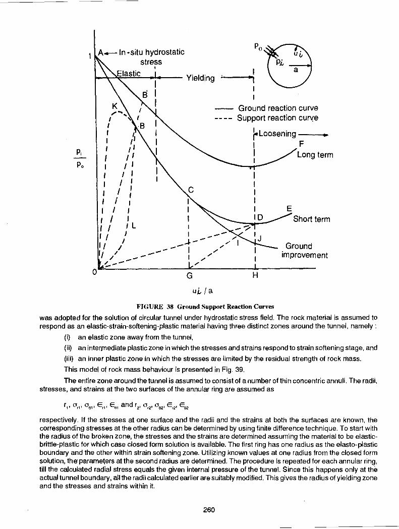
P,

Po

0

~ ...... I "" I

II ,'1 I 1 I I I 1

I I I 1 I I I I 1

I I I I I : I I I I I I I I I L I I 1

II I .J.--

1 --I - / / II I -- I

/ --­~ .............

G

/ /

uL I a

/

Ground reaction curve Support reaction cur~e

/

"' I

r Loosening --• I F I Longterm I

H

Ground improvement

FIGURE 38 Ground Support Reaction Curves

was adopted for the solution of circular tunnel under hydrostatic stress field. The rock material is assumed to respond as an elastic-strain-softening-plastic material having three distinct zones around the tunnel, namely:

{i) an elastic zone away from the tunnel,

{ii) an intermediate plastic zone in which the stresses and strains respond to strain softening stage, and

{iii) an inner plastic zone in which the stresses are limited by the residual strength of rock mass.

This model of rock mass behaviour is presented in Fig. 39.

The entire zone around the tunnel is assumed to consist of a number of thin concentric annuli. The radii, stresses, and strains at the two surfaces of the annular ring are assumed as

respectively. If the stresses at one surface and the radii and the strains at both the surfaces are known, the corresponding stresses at the other radius can be determined by using finite difference technique. To start with the radius of the broken zone, the stresses and the strains are determined assum·1ng the material to be elastic­brittle-plastic for which case closed form solution is available. The first ring has one radius as the elasto-plastic boundary and the other within strain softening zone. Utilizing known values at one radius from the closed form solution, the' parameters at the second radius are determined. The procedure is repeated for each annular ring, till the calculated radial stress equals the given internal pressure of the tunnel. Since this happens only at the actual tunnel boundary, all the radii calculated earlier are suitably modified. This gives the radius of yielding zone and the stresses and strains within it.

260

M

b (j 3 = Constant ....

b

+

v

+

FIGURE 39 Material Ilehaviour Model used by Brownet al (1983)

Brown eta/'s (1983) method of calculating ground convergence, based on finite difference techniques, has been modified to incorporate integration within the thin annular rings. Comparing the results for particular cases for which closed form solutions are available, it is seen that the modified procedure is more efficient as the iteration cycle converges faster and the results are closer to those obtained from closed form solutions.

The finite difference approximation gives

r2 = r, [ ~ EOl Er1 Er2 l Eo:z Er1 Er2 ... (42)

The exact integration gives

r2 = r1 r, .. , [(h

+ 1) E02 (h - 1) 2 E01 2

... (43)

Experimental evidence from tests conducted using a stiff testing machine shows that the relationship

261

between axial and radial strains in a failing rock is non-linear. The following·reilationship has been used for calculating tunnel convergences;

E3

=-h.E1

where h = h1 - h2 ( 1 - : 1; )

E3

= minor principal strain in yielding zone,

E1

= corresponding major principal strain,

h, = constant, equal to initial tangent of E1

vs E3

curve,

h2

=constant by which amount, the tangent to E1

vs E3

reduces as E1

goes to infinity, and

E18

=major principal strain corresponding to peak yield strength.

... (44}

With the modified approach of Brown eta/ (1983) as suggested by Sharma (1985), a parametric study of various factors affecting ground convergence, radius of broken zone and stress distribution was carried out in order to establish the relative importance of these factors in the design of tunnel. The influence of the following parameters was studied for a range of values of

0.3 other assumed data m = o. 7 s = o. 004

Oc= 27.5 MPa Em= 1380.0 MPa

~ = 0.25 Po = 3.3 MPa m, = 0.025 s = 0.0

r

h,=2.5 h2=1.5

0.2

0.1

0.0 ...__ ______ ......__ _____ ~ 2.0 3.0 4.0

u -'X 10·3

r,

FIGURE 40 Influence of Extent of Ground Softening on Tunnel Closure

262

{i) peak strength,

{ii) residual strength,

{iii) modulus of elasticity,

{iv) rate of strain softening; defined by a' as the ratio of principal strain to reach residual strength to the strain required to reach peak strength, and

{v) dilation characteristics of rock mass.

The following are some of the salient observations :

{i) The convergence curve and the radius of broken zone are marginally influenced by changes in the dilation characteristics of rock mass and ratio of peak strength to residual strength for varying values of residual strength with constant peak strength.

{ii) The rate of strain softening as defined by a' has significant influence on ground reaction curve· and the radius of broken zone for values of a' less than 3.5. But, for values of a'= 3.5 to infinity, the influence is negligible. Most fractured rock masses, particularly in the Himalayan region, exhibit a value, of a' greater than 3.5. Therefore, the influence of rate of strain softening from peak to residual stage may not be important, as shown in Fig. 40.

{iii) The peak strength and modulus of elasticity have pronounced effect on the ground reaction curve and radius of broken zone around the circular tunnel. Figure 41 shows typical strength envelopes in terms of Mohr-Coulomb criterion for uniaxial compressive strength of intact rock of 27.5 MPa. The corresponding values of m and s as per Hoek-Brown criterion are also

~ 11.. ~ CJ) C/) Q) ..... ..... C/)

..... ~ Q) ..c (f)

8

7

6

5

4

3

2

0 1

o Very high strength o' High strength l:l Average strength • Poor strength • Very poor strength

2 3 4 5

Normal stress, MPa

6 7

FIGURE 41 El)uivalent Mohr-Coulomb Envelopes for Different Rock Masse~

263

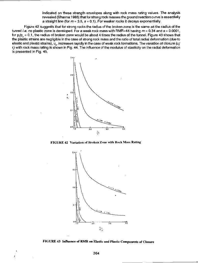
indicated on these strength envelopes along with rock mass rating values. The analysis revealed (Sharma 1985) that for strong rock masses the ground reaction curve is essentially a straight line (form= 3.5, s = 0.1 ). For weaker rocks it decays exponentially.

Figure 42 suggests that for strong rocks the radius of the broken zone is the same as the radius of the tunnel i.e. no plastic zone is developed. For a weak rock mass with RMR=44 having m = 0.34 and s = 0.0001, for P/Po = 0.1, the radius of broken zone would be about 4 times the radius of the tunnel. Figure 43 shows that the plastic strains are negligible in the case of strong rock mass and the ratio of total radial deformation (due to elastic and plastic strains), u;,• increases rapidly in the case of weak rock formations. The variation of closure (u/ r;) with rock mass rating is shown in Fig. 44. The influence of the modulus of elasticity on the radial deformation is presented in Fig. 45.

!

P,

P.

04

'· r.

FIGURE 42 Variation of Broken Zone with Rock Mass Rating

0.4

20 30 4.0

FIGURE 43 Innuence of RMR on Elastic and Plastic Components of Closure

264

0.4 Oth•r assum•d data Em : 1380 MPa J.!: 0.25 m, : 0.025 s,: 0.0 01 = 3.5 h1 :2.5 h2 : 1. 5 CJC :27.5 MPa p

0 : 3.3MPa rl : S,JJm

FIGURE 44 Innuence of RMR on Tunnel Closure

u. -'X 10·3 r. ,

I

FIGURE 45 Innuence of Modulus of Rock on Closure

265

0.3

Rock cover = 280 m

Dia. of Tunnel = 3.0 m

Em, = . 1 x 1 0 4 kg/cm2

RMR = 34

0.1

4.0 kg/ cm2

(I)

(II)

(iiQ

Measured

P, = 2.3 - 4.0 kg/cm2

U.= 94 mm I

Predicted (Eqn. 45)

P; = 3. 75 ; 4. 0 kg/cm2

u. = 86.3; 97.5 mm I

Terzaghi

P, = 3.3 to 7.4 kg/cm2

0.05 ------------"--------~-r---------------------- I 3.75kg/ cm2

0 10 20 30

86.3 em

40 50

u -'X 10·3

r,

97.5cm

60 70 80 90 100

FIGURE 46 Ground Convergence Curve - Yamuna Hydel Project • Stage 2, Part II

APPROXIMATE RELATION FOR GROUND REACTION CURVE

In order to avoid rigorous calculations as suggested in the foregoing, a simple approximate expression is suggested linking U/r

1 with P/Po through oc of intact rock, (o, · u)m of rock mass and Jn EIKn, where Jn =number

of joints per meter length, E =modulus of elasticity of intact rock, and Kn =joint stiffness.

From theoretical analysis (Singh, 1973), · E 1 K = ( EEm _ ~) ln n I

This reJ..ationship is given as

where

=

J = Jn E I ~n'

1 + 0. 0525 J R 1

(P; I Po )R 2

[ l 0.5

( o; - a 3 1 I In Po

and

'[ ( l~ _ Oj ]0.15 R2 = 1 I In

Po

... (45)

The values of (u, -o) of rock mass can be obtained from Eq. 17 whereas EjE may be obtained from Eq. 24 or Eq. 25 or from the tests conducted in the laboratory and field to evaluate Jn, E and Kn.

A comparison of radial deformation obtained from this simple empirical Eq. 45 with the rigorous approach presented in Table 15 suggest its relability.

A comparsion of ground reaction response predicted for Giri and Yamuna tunnels with the observed values of support pressures and actually measured radial deformations is shown in Fig. 46 and 47. The comparison is definitely encouraging. Even in the Clise of the Kielder exprimental tunnel, a reasonably good agreement has been observed as shown in Fig.48.

266

P;

Po

0.2

0.1

0

Rock cover = 380 m

Ex. Dia. = 2.1 m

E = 10 5 kg/em' RMR = 34

(I) Measured

Pi= 2.24 kg/cm2

U. =55 em I

(II) Predicted (Eqn. 45)

Pi= 1.9 ; 4.75 kg/cm2

ui = 21 ; 57.1 em (iiO Terzaghi

Pi = 2.3 - 4.4 kg/cm2

1~ !_g~m2 ____ !- ______ =-:-::-=:-:_:-:::-:_=--....----

40 21cm

FIGURE 47 Ground

0.4

\ I

0.3

0.2

p

0.1

60 120 57.1 em

u -'X 1Q-3

r. I

Con vergence Curve- Girl Hydel Projet

By experiments at site

By rigorous calculations neglecting gravity By rigorous calculations incorporating gravity effect

By correlation

160

FIGURE 48 Comparison Between Experimental and Calculated Ground Reaction Curves-- Kielder Experimental Tunnel, U.K.

267

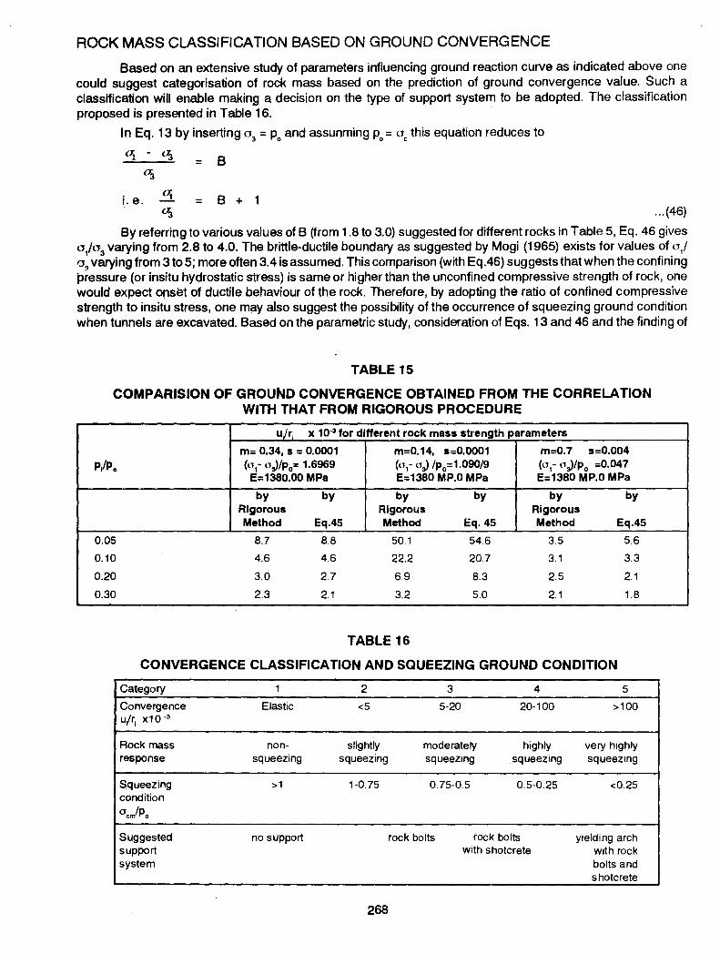
ROCK MASS CLASSIFICATION BASED ON GROUND CONVERGENCE

Based on an extensive study of parameters influencing ground reaction curve as indicated above one could suggest categorisation of rock mass based on the prediction of ground convergence value. Such a classification will enable making a decision on the type of support system to be adopted. The classification proposed is presented in Table 16.

In Eq. 13 by inserting o3

= Po and assunming Po= oc this equation reduces to

l}j_ - Oj = B

OJ

i. e. o; = B + 1

OJ ... (46)

By referring to various values of B (from 1.8 to 3.0) suggested for different rocks in Table 5, Eq. 46 gives o,to3 varying from 2.8 to 4.0. The brittle-ductile boundary as suggested by Magi (1965) exists for values of u,l a~ varying from 3 to 5; more often 3.4 is assumed. This comparison (with Eq.46) suggests that when the confining pressure (or insitu hydrostatic stress) is same or higher than the unconfined compressive strength of rock, one would expect onset of ductile behaviour of the rock. Therefore, by adopting the ratio of confined compressive strength to insitu stress, one m<3,y also suggest the possibility of the occurrence of squeezing ground condition when tunnels are excavated. Based on the parametric study, consideration of Eqs. 13 and 46 and the finding of

TABLE15

COMPARISION OF GROUND CONVERGENCE OBTAINED FROM THE CORRELATION WITH THAT FROM RIGOROUS PROCEDURE

u/r x 10·3 for different rock mass strength parameters

m= 0.34, s = 0.0001 m=0.14, s:0.0001 m:0.7 s:0.004

P/Po (o1- oJ/p0= 1.6969 (u1- oJ /p0:1.090/9 (u1- uJ/p0 :0.047 E=1380.00 MPa E=1380 MP.O MPa E:1380 MP.O MPa

by by by by by by Rigorous Rigorous Rigorous Method Eq.45 Method Eq.45 Method Eq.45

0.05 8.7 8.8 50.1 54.6 3.5 5.6

0.10 4.6 4.6 22.2 20.7 3.1 3.3

0.20 3.0 2.7 6.9 8.3 2.5 2.1

0.30 2.3 2.1 3.2 5.0 2.1 1.8

TABLE 16

CONVERGENCE CLASSIFICATION AND SQUEEZING GROUND CONDITION

Category 1 2 3 4 5

Convergence Elastic <5 5-20 20-100 >100 u(r1 x10 ·3

Rock mass non- slightly moderately highly very highly response squeezing squeezing squeezing squeezing squeezing

Squeezing >1 1-0.75 0.75-0.5 0.5-0.25 <0.25 condition 0 crriPo

Suggested no support rock bolts rock bolts yielding arch support with shotcrete with rock system bolts and

shotcrete

268

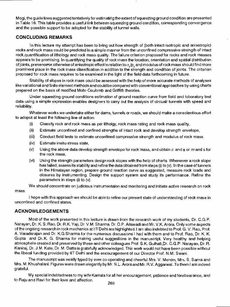
Mogi, the guide lines suggested tentatively for estimating the extent of squeezing ground condition are presented in Table 16. This table provides a useful link between squeezing ground condition, corresponding convergence and the possible support to be adopted for the stability of tunnel walls.

CONCLUDING REMARKS

In this lecture my attempt has been to bring out how strength of (both intact-isotropic and anisotropic) rocks and rock mass could be predicted in a simple manner from the unconfined compressive strength of intact rock,quantification of lithology and rock mass quality. The failure criterion proposed for rocks and rock masses appears to be promising. In quantifying the quality of rock mass the location, orientation and spatial distribution of joints, presenceror otherwise of anisotropic effect in relation to ajpo and modulus of rock mass should find more prominent place in the rock mass classification in addition to the strength and condition of joints. The criterion proposed for rock mass requires to be examined in the light of the field data forthcoming in future.

Stability of slopes in rock mass could be assessed with the help of more accurate methods of analyses like variational and finite element methods and could be compared with conventional approaches by using charts prepared on the basis of modified Mohr-Coulomb and Griffith theories.

Under squeezing ground conditions estimation of ground reaction curve from field and laboratory test data using a simple expression enables designers to carry out the analysis of circualr tunnels with speed and reliability.

Whatever works we undertake either for dams, tunnels or roads, we should make a conscientious effort to adopot at least the following line of action:

mass.

(i) Classify rock and rock mass as per litholgy, rock mass rating and rock mass quality,

(ii) Estimate unconfined and confined strengths of intact rock and develop strength envelope,

(iii) Conduct field tests to estimate unconfined compressive strength and modulus of rock mass.

(iv) Estimate insitu stress state,

(v) Using the above data develop strength envelope for rock mass, and obtain c and cp or m and s for the rock mass,

(vi) Using the strength parameters design rock slopes with the help of charts. Whenever a rock slope has failed, assess its stability and refine the data obtained from steps (i) to (v).lnthe case of tunnels in the Himalayan region, prepare ground reaction curve as suggested, measure rock loads and closures by instrumenting. Design the support system and study its performance. Refine the parameters in steps (i) to (v).

We should concentrate on judicious instrumentaion and monitoring and initiate active research on rock

I hope with this approach we should be able to refine our present state of understanding of rock mass in unconfined and confined states.

ACKNOWLEDGEMENTS

Most of the work presented in this lecture is drawn tram the research work of my students, Dr. C.G.P. Narayan, Dr. K. S. Rao, Dr. R.K. Yaji, Dr. V.M. Sharma. Dr. O.P. Ailawadi and Mr. V.K. Arora. Only some aspects of the ongoing research in rock mechanics at liT Delhi are highlighted.! am also indebted to Prof. G. V. Rao, Prof. A. Varadarajan and Dr. K.G.Sharma for the numerous discussions I had with them and to Prof. Rao, Dr. K. K. Gupta and Dr. K. G. Sharma for making useful suggestions in the manuscript. Very healthy and helping atmosphere created and preserved by these and other colleagues Prof. S.K. Gulhati,Dr. C.G.P. Narayan, Dr. R. Kaniraj, Dr. J.M. Kate, Dr. M. Datta is gratefully acknowledged. Thi~ work would not have been possible without the liberal funding provided by liT Delhi and the encouragement of our Director Prof. N.M. Swani.

The manuscript was neatly typed by ever co-operating and cheerful Mrs. V. Menon, Mrs. S. Sarna and Mrs. M. Khushalani. Figures were drawn elegantly by Mr. N.L. Arora and Mr. R.V. Aggarwal. To them I am indeed grateful.

My special indebtedness to my wife Kamala for all her encouragement, patience and forebearance, and to Raju and Ravi for their love and affection.

269

REFERENCES AILAWADI, O.P. (1985) : ''Eiasto-plastic Finite Element Analysis of Rock Slopes". Ph.D. Thesis, Indian Institute of Technology, Delhi, India.

ALDRICH, M.J. (1969) :"Pore Pressure Effects on Berea Sandstone subjected to Experimental Deformation" Bull. Geol. Soc. Am., 80; 1577-1586.

ATTEWELL, P.B. and SANDFORD, M.R. (1974): "Intrinsic Shear Strength of a Brittle, Anisotropic Rock. I. Experiemen­tal and Mechanical Interpretation". lnt Jnl. Rock Mech. Min. Sci. 11; 423-430.

BARTON, N. R. (1970) :"A Low Strength Material for Simulation of the Mechanical Properties of Intact Rock in Rock Mechanics in Models." Proc. 2nd Congr. Rock Mech., Belgrade, 3-15: 90-110.

BARTON, N.R. (1973) : "Review of Shear Strength Criterion for Rock Joints". Eng g. Geol.. 7 : 287-332.

BARTON, N.R. and CHOUBEY, V.D (1977): "The Shear Strength of Rock Joints in Theory and Practice." Rock Mech., 10:1:1-54.

BARTON, N.R., LIEN, R. and LUNDE, J (1974) : "Engineering Classification of Rock Masses for the Design ofTunnel Support." Rock Mech., 6:4:189-236.

BELL, F.G. (1978) :"Petrological Factors Relating to Porosity and Permeability in the Fell Sandstones "Ort. Jnl. Engg. Geol., 11: 113-126.

BIENIAWASKI, Z. T. (1973) : "Engineering Classification of Jointed Rock Masses" Trans. South Afircan lnstn. C1v. Engr., 15:12:335-344.

BIENIAWSKI, Z.T. (1974) : "Geomechanics Classification of Rock Masses and its Application in Tunneling". Proc. 3rd Int. Congr Rock Mech, Denver, Part A, pp. 27-32.

BIENIAWSKI, Z.T. (1978) : "Determining Rock Mass Deformability: Experience from Case Histories." Int. Jnl. Rock Mech. Min. Sci., 15 :237-248.

BISHOP, A.W. (19t>S) : "The Use of the Slip Circle in the Stability Analysis of Slopes." Geotechnique, 5:1 7-17.

BOOZER, G. D., HILLER, K. and SERDENGECTI, S. (1962): "Effects of Pore Fluids on the Deformation Behaviour of Rocks Subjected to Triaxial Compression." Proc. Symp. Rock Mech., 5th, Pergamon, p. 578.

BRACE, W.F. (1964) :"Brittle Fracture of Rocks, State of Stress in the Earth's Crust." Judd, WR .. ed., Elsev1er, New York, pp. 111-174.

BROCH, E. (1974) :'The Influence of Water on Some Rock Properties". Advances in Rock Mech., National Academy of Science, pp. 33-38.

BROCH, E. and FRANKLIN, JA (1972): "The Point Load Strength Test." Int. J. Rock Mech. Min. Sci. 9:669-697

BROOK, N. (1979) :"Estimating the Triaxial Strength of Rocks." Int. J. Rock Mech. Min. Sci. Geomech. Abstr., 16261-264.

BROWN, C.B. and KING, I.P. (1966) : "Automatic Embankment Analysis; Equilibrium and Instability Conditions." Geotechnique, 16:3:209-219.

BROWN. ET., BRAY, J.W., LADANYI, B. and HOEK. E. (1983) :"Ground Response Curves for Rock Tunnels." Jnl. Geotech. Eng g. ASCE, 109 :1:15-39.

CHENVERT, M.E. and GATLIN, C. (1965): "Mechanical Anisotropic of a Laminated Sedimentary Rocks" Soc. Pet. Engrs. J., pp. 67-77.

CHERNOVS'KO, F.L. (1965) : "A Local Variational Method for the Numencal Solutions of Variational Problems." U.S.S.R. Computational Mathematics and Mathematical Physics, 5:4:234-241.

CHUGAEV. R.R. (1964): "Stability Analysis of Earth Slopes, Jerusalem". Trans. from Russian, Israel Programme of Scientific Translations, 1966.

COLLIN, A. (1846) : "Giissement Spontanes des Terrains Argileux," Paris, Charilian Goeury and Dulmont (English Translation Pub I. 1956 by Uni-Toronto Press).

COOL! NG, I. F. and GOLDER, H. Q. (1942) : "The Analysis of the Failure of an Earth Dam during Construction." Jnl I nstn. Civ. Engrs., 19:38-55.

COULOMB, C. A. (1773) : "Application des Ragles de Maximis at Minims a Quelques Problems de Statique Relatifs a I' Architecture", Memoires de Savants Etrangers de I' Academic des Science de Paris, 7:343-382.

DAEMEN, J.J.K. (1975): "Tunnel Support Loading Caused by Rock Failure". Ph.D. Thesis, University of Minnesota, Minnesota, USA.

DEERE, D.U. (1964) : "Technical Description of Rock Cores for EnginP.oring Purposes." Rock Mech. and Engg. Geology, 1:1:17-22.

DEERE, D.U. and MILLER, R.P. (1966): "Engineering Classification and Index Properties for Intact Rock." Tech. Rept.

270

No. AFWL-TR-65-116, Air Force Weapons Lab, New Mexico.

DONATH, F.A. (1964) : "Strength Variation and Deoformational Behaviour of Anisotrophic Rocks." State of Stress in the Earth's Crust, W.R. Judd, ed., Am. Elsevier Publ. Comp., New York, pp. 281-298.

DONATI-1, FA (1970) :"Some Information Squeezed Out of Rock", Am. Scientist, 58:54-72.

DONATH, F.A. (1972): "Faulting Across Discontinuities in Anisotropic Rock, Stability of Rock Slopes", Proc 13th Symp. Rock Mech., Urbana, New York, Am. Soc. Civ. Eng., pp. 753-772.

DONATH, F.A. and FRUTH; L.S. (1971) : "Dependence of Stress rate Effects on Deformation Mechanism and Rock Type." J. Geol., 79:347.

DUBE, A K. (1979) : "Geomechanical Evaluation of Tunnel Stability under Failing Rock Conditions in a Himalayan Tunnel". Ph.D. Thesis, University of Roorkee, India.

FELLENIUS, W. (1936) : "Calculation of the Stability of Earth Dams", Trans. 2nd Cong. on Large Dams, Vol. 4, Washington.

FRANKLIN, J.A. (1971): "Triaxial Strength of Rock Materials". Rock Mech., 3:86-98.

GELFAND, I.M. and FOMIN, S.V. (1963): "Calculus of Variations," Prentice-Hall, Inc., Englewood Cliffs. New Jersey, pp. 54-63.

GNIRK, PF. and CHEATHAN, J.B. (1965) : "An Experimental Study of Single Bit-Tooth Penetration into Dry Rock at Confining Pressures of 0 to 5000 psi," Soc. Pet. Engrs. J., 5:2:117-130.

GOLDS TEl N, I. M. (1969) : "Application of Calculus of Variations to Investigations of Bases and Slopes." Soil Mech. and Foundation Eng g., 1:3-9.

GRIGGS, D.T. (1936) : "Deformation of Rock Under High Confining Pressure". J. Geol, 44:541-577.

GRIGGS, D.T., TURNER, F.J. and HEARD, H.C. (1960) :"Deformation of Rocks at 5oo• to 8oo·c., in Rock Deformation". Geol Soc. Am. Mem., 79: 39-104.

HANOI N, J. and HAGER, R. V. (1957) : "Experimental Deformation of Sedimentary Rocks under Confining Pressure: Tests at Room Temperature on Dry Samples." Bull. Am. Assoc. Petrol,. Geol., 41:1-50.

HANDIN, J. and HAGER, R.V. (1958) : "Experimental Deformation of Sedimentary Rocks under High Confining Pressure: Tests at High Temperature." Bull. Am. Soc. Petrol Geol., 42:2894-2934.

HAN DIN, J., HAGER, R.V., FRIENDMAN, M. and FEATHER, J.N. (1963): "Experimental Deformation of Sedimentary Rocks under Confining Pressure: Pore Pressure Effects." Bull. Am. Assoc. Petrol. Geol., 47:717-755.

HOEK, E. (1968) : "Brittle Failure of Rock". Rock Mechanics in Engineering Practice, Stagg and Zienkiewicz, eds., Wiley, London, pp. 99-124.

HOEK, E. (1970): "Estimating the Stability of Excavated Slopes inOpencast Mines". Trans. lnst. Mining and Metallurgy, London, 79 : A 1 09-A 131.

HOEK, E. (1983) :"Strength of Jointed Rock Masses." Geotechnique, 33:3:187-223.

HOEK, E. and BRAY, J. (1977) : "Rock Slope Engineering." lnst. Mining and Metallurgy, London, (2nd Edn.).

HOEK, E. and BROWN, E. T. (1980): "Underground Excavations in Rock". Institution of Mining and Metallurgy, London.

HOEK, E. and BROWN, E.T. (1983): "Empirical Strength Criterion for Rock Masses", Jnl. Geotch. Engg. Div., ASCE, 1 06: GT9: 1 01 3-1 035.

HOFER, K.H. and THOMA, K. (1968): "Triaxial Tension Salt Rocks." Int. Jnl. Rock Mech. Min. Sci., Geotech. Abstr., 5:195-203.

HORINO, F.G. and ELLIKSON, M.L. (1970) : "A Method of Estimating the Strength of Rock Containing Planes of Weakness," U.S. Bureau Mines Report Investigation 7449.

HOSHINO, K., KOIDE, H., INAMI, K., IWAMURA, S. and MITSUI, S. (1972) :"Mechanical Properties of Japanese Tertiary Sedimentary Rocks under High Confining Pressure." Geol. Surv .. Jpn., Rep. No. 244, pp. 1-200.

HOUPERT, R. (1970) :"La Resistance a low Rupture des Roches on Compression Simple". Proc. 2nd Congr. Int. Rock Mech., Belgrade, 2:49-55.

HUTCHINSON, J.N. (1961) :"A Landslide on a Thin Layer of Quick Clay at Furre, Central Norway". Geotechnique, 11 :2:69-94.

JAEGER, J.C. (1960): "Shear Failure of Anisotropic Rocks," Geol. Mag., 97:65-72.

JAEGER, J.C. (1971) : "Friction of Rocks and Stability of Rock Slopes". Geotechnique, 21:2:97-134.

JAEGER, J.C. and COOK, N.G.W. (1979): "Fundamentals of Rock Mechanics," Chapman and Hall, London, p. 593.

JANBU, N. (1954) : "Application of Composite Slip Surfaces for Stability Analysis". Proc. European Cont., Stability of Earth Slopes, Stockholm, 3:43-49.

271

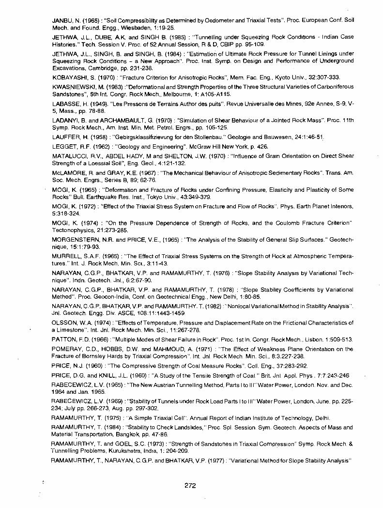
JANBU, N. (1965) : "Soil Compressibility as Determined by Oedometer and Triaxial Tests". Proc. European Conf. Soil Mech. and Found. Engg., Wiesbaden, 1:19-25.

JETHWA, J.L., DUBE, AK. and SINGH B. (1985) : "Tunnelling under Squeezing Rock Conditions - Indian Case Histories." Tech. Session V. Proc. of 52 Annual Session, R & D, CBIP pp. 95-109.

JETHWA, J.L., SINGH, B. and SINGH, B. (1984) :"Estimation of Ultimate Rock Pressure for Tunnel Linings under Squeezing Rock Conditions - a New Approach". Proc. lnst. Symp. on Design and Performance of Underground Excavations, Cambridge, pp. 231-238.

KOBAYASHI, S. (1970) : "Fracture Criterion for Anisotropic Rocks", Mem. Fac. Eng., Kyoto Univ., 32:307-333.

KWAS.NIEWSKI, M. (1983) :"Deformational and Strength Properties ofthe Three Structural Varieties of Carboniferous Sandstones", 5th Int. Congr. Rock Mech., Melbourne, 1: A105-A115.

LABASSE, H. (1949). "Les Pressons de Terrains Author des puits". Revue Universalle des Mines, 92e Annee, S-9, V-5, Mass., pp. 78-88.

LADANYI, B. and ARCHAMBAULT, G. {1970): "Simulation of Shear Behaviour of a Jointed Rock Mass". Proc. 11th Symp. Rock Mech., Am. lnst. Min. Met. Petrol. Engrs., pp. 105-125.

LAUFFER, H. (1958) : "Gebirgsklassifizievung for den Stollenbau." Geologie and Bauwesen, 24:1 :46-51_.

LEGGET, R.F. {1962) :"Geology and Engineering". McGraw Hill New York, p. 426.

MATALUCCI, R.V., ABDEL HADY, M and SHELTON, J.W. (1970): "Influence of Grain Orientation on Direct Shear Strength of a Loessial Soil", Eng. Geol., 4:121-132.

McLAMORE, R. and GRAY, K.E. (1967) : "The Mechanical Behaviour of Anisotropic Sedimentary Rocks". Trans. Am. Soc. Mech. Engrs., Series B, 89; 62-76.

MOGI, K. (1965) : "Deformation and Fracture of Rocks under Confining Pressure, Elasticity and Plasticity of Some Rocks" Bull. Earthquake Res. lnst., Tokyo Univ., 43:349-379.

MOGI, K. (1972) : "Effect of the Triaxial Stress System on Fracture and Flow of Rocks''. Phys. Earth Planet Interiors, 5:318-324.

MOGI, K. (1974) : "On the Pressure Dependence of Strength of Rocks, and the Coulomb Fracture Criterion" Tectonophysics, 21:273-285.

MORGENSTERN, N.R. and PRICE, V.E., {1965) : "The Analysis of the Stability of General Slip Surfaces." Geotech­nique, 15:1:79-93.

MURRELL, S.A.F. (1965) : "The Effect of Triaxial Stress Systems on the Strength of Rock at Atmospheric Tempera­tures." Int. J. Rock Mech. Min. Sci., 3:11-43.

NARAYAN, C.G.P., BHATKAR, V.P. and RAMAMURTHY, T. (1976) :"Slope Stability Analysis by Variational Tech­nique". lndn. Geotech. Jnl., 6:2:67-90.

NARAYAN, C.G.P., BHATKAR, V.P. and RAMAMURTHY, T. (1978) : ''Slope Stability Coefficients by Variational Method". Proc. Geocon-lndia, Cont. on Geotechnical Engg., New Delhi, 1:80-85.

NARAYAN, C.G.P. BHATKAR, V.P. and RAMAMURTHY. T. {1982): ''Nonlocal Variational Method in Stability Analysis". Jnl. Geotech. Engg. Div. ASCE, 108:11:1443-1459.

OLSSON, W.A. (1974) : "Effects of Temperature, Pressure and Displacement Rate on the Frictional Characteristics of a Limestone". Int. Jnl. Rock Mech. Min. Sci., 11:267-278.

PATTON, F. D. {1966): "Multiple Modes of Shear Failure in Rock". Proc. 1st ln. Congr. Rock Mech., Lisbon, 1:509-513.

POMERAY, C.D., HOBBS, D.W. and MAHMOUD, A. {1971) : "The Effect of Weakness Plane Orientation on the Fracture of Bornsley Hards by Triaxial Compression". Int. Jnl. Rock Mech. Min. Sci., 8:3:227-238.

PRICE, N.J. {1960) : "The Compressive Strength of Coal Measure Rocks". Coli. Eng., 37:283-292.

PRICE, D. G. and KNILL, J.L. {1960) : "A Study of the Tensile Strength of Coal." Brit. Jnl. Appl. Phys., 7:7:243-246.

RABECEWICZ, L.V. (1965) :"The New Austrian Tunnelling Method, Parts I to Ill" Water Power, London. Nov. and Dec. 1964 and Jan. 1965.

RABECEWICZ, L.V. {1969) :"Stability ofTunnels under Rock Load Parts I to Ill" Water Power, London, June, pp. 225-234; July pp. 266-273, Aug. pp. 297-302.

RAMAMURTHY, T. (1975) : "A Simple Triaxial Cell". Annual Report of Indian Institute of Technology, Delhi.

RAMAMURTHY, T. {1984) : "Stability to Check Landslides," Proc Spl. Session. Sym. Geotech. Aspects of Mass and Material ~ransportation, Bangkok, pp. 47-86.

RAMAMURTHY, T. and GOEL, S.C. (1973) : "Strength of Sandstones in Triaxial Compression" Symp. Rock Mech. & -runnelling Problems, Kurukshetra, India, 1: 204-209.

RAMAMURTHY, T., NARAYAN, C.G.P. and BHATKAR, V.P. (1977): "Variational Method for Slope Stability Analysis"

272

Proc. 9th Int. Cont. SMFE, Tokyo, 2:139-142.

RAMAMURTHY, T., RAO, G.V. and RAO, K.S. (1985): ''A Strength Criterion for Rocks." Proc. lndn. Geotech, Cont., Roorkee, Vol. 1, pp. 59-64.

RAMAMURTHY., T., SHARMA, K.G. and AILAWADI, O.P. (1985): "Eiastoplastic Finite Element Analysis of Slopes in Rock Mass." Int. Cont. on Finite Element Computational Mechanics, Bombay, 1:291-300.

RAO, K .. S., (1984) : "Strength and Deformation Behaviour of Sandstones". Ph.D. Thesis, Indian Institute ofT echnology, Delhi, India.

RAO., K.S., RAO, G.V. and RAMAMURTHY, T. (1985): "Rock Mass Strength from Classification". Proc. of Workshop on Engg. Classification of Rocks, Central Board of Irrigation and Power, New Qelhi, pp. 27-50.

RUMMEL, F. and FAIRHURST, C. (1970): "Determination of the Post Failure Behaviour of Brittle Rock using a Se!"¥o· controlled Testing Machine". Rocks Mech, 2:189-204.

RZHEVSKY. V. and NOVIK, G. (1971): "The Physics of Rocks". MIA Publishers, Moscow, p. 320.

SCHNEIDER, H.J. (1976): "Friction .and Deformation Behaviour of Rock Joints." Rock Mech., 8:169-184.

SCHWARTZ, A. E. (1964): "Failure of Rock in the Triaxial Shear Test", Proc. of the 6th Symp. on Rock Mech., Rolla, MO, pp. 109-151.

SEI FEAT, K. E. (1969) : "Strength of Adirondack Anorthosite at Elevated Temperatures and Pressures." Geol. Am. Bull., 80; 10:2053-2059.

SERDENGECTI, S. and BOOZER, W.S. (1961): "The Effects of Strain Rate and Temperature on the Behaviour of Rocks Subjected to Triaxial Compression." Proc. 4th Symp. Rock Mech. Univ. Park, Penn., pp. 83-97.

SHARMA. V.M. (1985) :"Predication of Closure and Rock Loads for Tunnels in Squeezing Grounds". Ph.D. Thesis Indian Institute of Technology Delhi, India.

SHARMA, K.G., RAMAMURTHY, T. and AILAWADI, O.P. (1984) : "Eiasto-plastic Finite Element Analysis of Rock Slopes." Proc. 5th Int. Conf. Numeri, Methods in Geomech, Japan, 2; 981-987.

SINGH, B. (1973): "Continuum Characterization of Jointed RockMasses."lnt. Jnl. RockMech. Min. Sci. and Geomech. Abst., 1:4:311-349.

SINGH, B. (~ 978) : "Analysis and Design Techniques for Underground Structures" Proc. Geocon-lndia, Cont. on Geotech, Engr., New Delhi, 2:102-112.

SKEMPTION, A.W. (1964): "Long term Stability of Clay Slopes." Geotechnique, 14:2:77-101.

SMART, B.G.D., ROWLANDS, N. and ISAAC, A.K. (1982): "Progress Towards Estabilising Relationships between the Mineralogy and Physical Properties of Coal Measures Rocks."lnt. Jnl. Rock Mech. Min. Sci. and Geomech. Abstr., 19 : 81-89.

SOKOLOVSKY, V.V. (1960): "Statics of Soil Media". Butterworths Scientific Publication.

SPENCER, E. (1967) :"A Method of Analysis of the Stability of Embankments Assuming Parallellnterslice Forces". Geotechnique, 17:1:11-26.

SPENCER, E. (1968): "Effect of Tension on Stability of Embankments". Jnl. Soil Mech. & Found, Div., ASCE, 94: 5 :1159- 1173.

SPENCER, E (1969): "Cricular and Logarithmic Spiral Slip Surface." Jnl. Soil Mech. & Found. Div., ASCE, 95: 1 : 227-234.

SRIVASTAVA, L.S., GUPTA, R.P. and BEHARI, S. (1970) : "Evaluation of Strength from Porosity and Durability Measurement of Rocks". Jnl. Ind. Nat, Soc. Soil. Mech. l=ound. Eng., 9: 2 : 225-233.

STINI, I, (1950) : "Tu-nnelbaugeologie" Springer-Verlag, Vienna, p. 336.

STOW, R. L. (1969) : "Strength and Deformation Properties of Granite, Basalt, Limestone and Tuff at Various Load'1ng Rates". U.S. Army Corps. Eng., Waterways Expt. Station, Vicksburg, Miss., Misc. paper C-69-1.

STREET, Nand WANG, F.D. (1966): "Surface Potentials and Rock Strength". Proc. 1st Cong. Int. Soc. Rock Mech., Lisbon, 1 : 451-456.

SUBASH BABU, L., MARKANDEY, and ULABHAJE, A. V. (1977) : "Mineral Compositions and Strength Properties of some Sandstones from Singrauli Coal Fields." Jnl. Mines, Metals, Fuels, 25 : 7.

TAYLOR, D.W. (1948): "Fundamentals of Soil Mechanics". John Wiley Publications, New York.

TERZAGHI, K. (1946) : "Rock Tunnelling with Steel Supports." by proctor, R.V. and White, T.L., The Commercial Shearing and Stamping Co. Youngstown, Ohio.

VON KARMAN (1911) : "The Festigskeitsversuche under Auseitigem Druck". Zeits, Verein Deutsch. I ng., 55 : 17 49-1757.

VUTUKURI, V.S., LAMA. R. D. and SALUJA, S.S. (1974): "Hanbookon Mechanical Properties of Rock," voi.I-IV. Trans.

273

Tech. Publications.

WALSH, J. B. and BRACE, W. F. (1964) : "A Facture Criterion for Brittle Anisotropic Ro9ks," Geophysics Research Jnl., 69:3442.

WAWERSIK, W.R. and BRACE, W.F. (1971): "Post-failure Behaviour of a Granite and a Diabase." Rock Mech., 3:61-85.

WAWERSIK, W.R. and FAIRHURST, C. (1970) : "A Study of Brittle Rock Fracture in Laboratory Compression Experiments". Int. Jnl. Rock Mech. Min. Sci., 7 : 561-575.

WILHELMI. B. and SOMERTON, W.H. (1967): "Simultaneous Meausrement of Pore and Elastic Properties of Rocks u~der Triaxial Stress Conditions." Jnl. Soc. Petrol Eng., AIME, 7: 283-294.

WOLFSKILL, L.A. and LAMBE, T.W. (1957} :"Slide in the Siburua Dam." Jnl. Soil Mech. & Found Div. ASCE, 93:4 : 107-133.

YAJI, R.K. (1984): "Shear Strength and Deformation Response of Jointed Rocks." Ph.D. Thesis, Indian Institute of Technology, Delhi, India.

YUDHBIR, LEMANZA, W. and PRINZL, F. (1983): "An-Empirical Failure Criterion for Rock Masses," 5th Int. Congr. Pock Mech., Melbourne, 1 : B1-8.

ZIENKIEWICZ, O.C. and CORMEAU, I. C. (1974) : "Visco-plasticity-plasticity and Creep in Elastic Solids- A Unified Numerical Solution Approach". Int. Jnl. Numerical Methods in Eng g., 8 : 821-845.

274