
srf disp map - Technion
20
Transcript of srf disp map - Technion

Geometric Deformation-Displacement Maps �
Gershon ElberComputer Science Department
TechnionHaifa 32000, Israel
Email: [email protected]
Abstract
Texture mapping, bumpmapping, and displacement maps are central instruments in computer graph-
ics aiming to achieve photo-realistic renderings. In all these techniques, the mapping is typically one-
to-one and a single surface location is assigned a single texture color, normal, or displacement. Other
specialized techniques have also been developed for the rendering of supplementary surface details such
as fur, hair, or scales.
This work presents an extended view of these procedures and allows one to precisely assign a single
surface location with few continuously deformed displacements, each with possibly di�erent texture
color or normal, employing trivariate functions in a similar way to FFDs. As a consequence, arbitrary
regular geometry could be employed as part of the presented scheme as supplementary surface texture
details. This work also augments recent results on texturing and parameterization of surfaces of arbitrary
topologies by providing more exible control over the phase of texture modeling.
By completely and continuously parameterizing the space above the surface of the object as a trivari-
ate vector function, we are able, in this work, to not only control the mapping of the texture on the
surface but also to control this mapping in the volume surrounding the surface.
Additional Key Words and Phrases: Curves & Surfaces, Texture Mapping, Bump Mapping,
Trivariates, Deformations, Warping, FFD.
1 Introduction
Texture mapping [11] is an essential apparatus in computer graphics that increases the photo-realism of
any synthetic rendering scheme. A mapping is established from any point on the surface of the rendered
object into the texture space. The surface point is then assigned the color of the respective location found
in the texture space. In this paper we will be concentratating on the texture mapping techniques that
relate to shape alteration. The bump map [1, 11] is a �rst attempt to modulate the normals of the vertices
of the rendered objects instead of their assigned colors. Here also, at each surface location, we assign
a small perturbation to the normal, based on some mapping from that surface location to some normal
perturbation texture function. The bump mapping technique is highly successful in conveying a bumpy
shape while the geometry remains smooth. The illusion created by the bump mapping is quite convincing.
�The research was supported in part by the Fund for Promotion of Research at the Technion, IIT, Haifa, Israel.
1

Geometric Deformation-Displacement Maps Elber 2
Yet, in silhouetted areas the surface remains smooth and no casting of self shadows due to this bumpiness
can occur, since the geometry itself is not modi�ed.
Displacement maps [3, 11] take the next natural step and allow actual modi�cation of the surface.
Typically, this map is represented as a height �eld that modulates the amount each surface location is
elevated in one direction, typically the normal direction. Let S(u; v) be the surface to displace and let
n(u; v) be its unit normal �eld. Then, given a displacement as a scalar height �eld, d(u; v), the geometry
of the new, modulated, surface equals,
Sd(u; v) = S(u; v) + n(u; v)d(u; v): (1)
The computation or the approximation of the normal �eld of Sd(u; v) can be quite involved and is, in
general, considered a computationally complex task that hinders the use of such techniques in real time.
Since the partials of S(u; v) span the tangent plane of S, if regular,�@S@u; @S@v; n�can serve as a basis
for IR3and hence can be used to prescribe a displacement in an arbitrary direction. Nonetheless, typically
only one displacement direction can be prescribed per (u; v) surface location. This displacement is, in most
cases, in the normal direction.
In [15], an approach that introduces texels is proposed. Quoting from [15], \a texel is a three dimensional
array that holds the visual properties of a collection of micro-surfaces". The geometry is replaced by its
visual properties, gathering the scattering and re ectance functions. It is this concept that attempts to
model the volume above the surface that triggered this work. Trilinear texels are also used in [19]. Due
to the linearity of the texel, one surface location is assigned one displacement direction. The texels are
continuous but their normals are not. Similarly, because the base of the texel is a bilinear form, it is
impossible to precisely follow non linear polynomial surfaces. One advantage of the approach of [15, 19]
stems from its ability to ray trace the scene without the need to duplicate the geometry behind the texture
function, remapping the general ray, as it is traced, into the canonical texel. This approach can also handle
texture mapping that is one-to-many. That is, a single surface location can be mapped to several points
above the surface. In this work, we further extend this approach into non linear trivariate functions, as an
alternative scheme to better manage the space above the surface.
Three-dimensional supplementary details were also added to the surface of the object using other means.
Typically, this texturing process could be divided into two. In the �rst, the texture placement phase, the
locations at which the texture elements are to be placed are determined. A typical approach to texture
placement employs some kind of a parameterization. Then, in the second, the texture modeling phase, the
texture elements are locally molded to �t their �nal shape.
In [10], an attempt was made at creating three-dimensional details, such as scales or thorns, over the
surface. Natural cellular development was simulated in [10] toward texture generators, for the placement

Geometric Deformation-Displacement Maps Elber 3
phase of the individual elements. The texture modeling phase in [10] exploited a geometric modeler that
is parametric. Cellular texture generators as a tool for texture placement have been receiving signi�cant
attention recently, and for example, in [17] brick textures are investigated for architectural models.
The question of texture placement is of major concern in irregular polygonal meshes of arbitrary
topology, as is the question of seamless tiling of a repeatable texture over these domains. These questions
have, of late, captured the attention of researchers. For example, [24] employs a vector �eld over the
geometry to achieve this proper placement and [25] derives a parameterization and local tangents for each
vertex of the mesh, attempting to reach the same goal. Simulation of reaction-di�usion [23, 26] is another
scheme used to create textures for surfaces with no parameterization.
In this work, we extend the notion of displacement maps and relax several of its constraints. By using
non linear polynomial trivariate functions to derive the texture mapping function, continuous normal �elds
may be created. The presented approach employs the same tool as used in freeform deformations (FFD) [21,
4] and hence the resulting texture undergoes a displacement transformation as well as a deformation that
coerces it to follow the precise shape of the underlying surface. As a consequence, any geometry in IR3
could be employed as supplementary detail texture, making the texture modeling phase as general as it
can be. Moreover, any object can serve as the geometric deformation-displacement map (DDM) of itself,
forming a complete closure.
[10, 17, 23, 24, 25, 26] are samples from the state of art in this area of texture placement, which seeks
a proper distribution of the texture elements on the surface, whether a square texture tile, a thorn, a brick
or hair. Herein, we augment these techniques by providing extended texture modeling capabilities. Having
a proper texture placement, we allow the texture function to fully and smoothly encompass the third
dimension above the surface. That is, given a surface location to place the texture along, the DDM maps
the surface location to more than one textured or displaced point. Moreover, by having a complete and
continuous parameterization of the surface domain and above it, we are able to fully adapt the displaced
texture to the shape of the surface as well as o�er an e�cient estimation scheme for the normals of the
deformed and displaced geometry.
This paper is organized as follows. In Section 2, we portray the proposed displacement approach, and in
Section 3, we present our e�cient estimation scheme for the normals of the displaced surface. In Section 4,
some examples are presented and �nally, we conclude in Section 5.
2 Geometric Displacement Algorithm
Consider O, a given object to be textured and let S(u; v), u; v 2 [0; 1] be a regular parametric surface
on the boundary of O. Denote S(u; v) as the base-surface. Further, let n(u; v) be the unit normal �eld of

Geometric Deformation-Displacement Maps Elber 4
uv
w
B
)
S(u; v)
n(u; v)wT (u; v; w)
Figure 1: The trivariate T (u; v; w) function is de�ned above surface S(u; v).
S(u; v), pointing outside of O. Then, let (see Figure 1),
T (u; v; w) = S(u; v) + n(u; v)w; (2)
be a trivariate function. The three-dimensional parametric space of T is the in�nite box B: (u; v; w),
u; v 2 [0; 1], w > 0. T (u; v; w) parameterizes the volumetric neighborhood of S(u; v) and exactly equates
with S for w = 0.
De�nition 1 A point P is considered above base-surface S(u; v) if there exist (u0; v0; w0),
w0 > 0, such that P = T (u0; v0; w0). S(u0; v0) is denoted the support-position of P .
Similarly,
De�nition 2 A point P is considered below base-surface S(u; v) if there exist (u0; v0; w0),
w0 < 0, such that P = T (u0; v0; w0). S(u0; v0) is denoted the support-position of P .
Point P may be above one support-position of the base-surface and below another. Alternatively, a
point can be above (or below) two di�erent support-positions. Methods to detect and possibly eliminate
such singularities in FFD mappings and related applications are now known. Consider T : IR3 ) IR
3. T is
one-to-one (or regular) if and only if the determinant of the Jacobian of T never vanishes. This constraint
on the Jacobian was computed to detect singular conditions in FFDs in [12], and was symbolically derived
to extract the boundary of a sweep surface operation in [7].
In this work, we are mainly concerned with the volume near the surface, for small values of w, and
therefore such a singularity or dual support-position is expected to be uncommon. Furthermore, we seek
an algorithm that needs no inverse function evaluation, which is more e�cient, and completely circumvents
the computation di�culties that such a singularity might pose.
Given a bivariate parametric displacement texture function D(r; t) = (u(r; t); v(r; t); w(r; t)) 2 B, the
embedding of D in T yields (See Figure 2)
T (D) = T (u(r; t); v(r; t); w(r; t))
= S(u(r; t); v(r; t))+ n(u(r; t); v(r; t))w(r; t): (3)

Geometric Deformation-Displacement Maps Elber 5
D(r; t)
)
T (D)
Figure 2: The mapping of the geometric displacement D(r; t) using the trivariate function T (u; v; w).
For the special case where u = r and v = t, D(r; t) is reduced to the traditional displacement mapping
technique, becoming an explicit height �eld above the (r; t) = (u; v) plane. Equation (3) now assumes the
form of (see also Equation (1))
T (D) = T (r; t; w(r; t))
= S(r; t) + n(r; t)w(r; t); (4)
while w(r; t) serves as the height �eld displacement along the direction of the normal. Hence, the traditional
displacement mapping technique is a special, explicit case of the parametric form presented in Equation (3).
What can be gained by using the more general parametric displacement representation is the key question
we are about to examine as part of this work.
Trivariate functions were introduced to the graphics community in the much cited work of [21] on
warping applications. Trivariate functions were employed as mappings T : IR3 ! IR
3. Bending, stretching,
and warping operators were represented using trivariate functions that bent, stretched or warped a subspace
of IR3. The work of [21], that is also known as freeform deformations (FFD), has many derivations such
as the Extended FFD [4], and non tensor product FFD representations [18]. All these derivations share
the ability to embed a given object in the domain of the trivariate, and that object undergoes the same
non-linear transformation along with the entire subspace around the object.
While an exceptionally general and powerful object modi�cation operator, the di�cult question has
always been how can one intuitively derive the proper trivariate function to perform a certain warping
operation. In this work, we borrow these powerful capabilities of the trivariate functions as a warping tool
while the trivariate function is de�ned to follow the three-dimensional domain above the surface boundary
of object O, following Equation (2).
Two types of parametric displacement maps, D(r; t), could now be employed, types we denote covering
displacement maps and casual displacement maps:
De�nition 3 D(r; t) = (u(r; t); v(r; t); w(r; t)), r; t 2 [0; 1] is considered a covering displace-
ment map if 8u0; v0 2 [0; 1], 9r0; t0 2 [0; 1] such that u(r0; t0) = u0, v(r0; t0) = v0.

Geometric Deformation-Displacement Maps Elber 6
In other words, any displacement map that is onto, and hence spans the entire surface is a covering
displacement map. Clear examples of covering maps are the traditional bump and displacement maps. A
covering displacement map can be discontinuous in w(r; t) and hence still present gaps in its range.
De�nition 4 D(r; t), r; t 2 [0; 1] is considered a casual displacement map if it is not a covering
displacement map.
If D(r; t) is not a covering displacement map, the base-surface will not be replaced by the displacement
map, but will merely be augmented by it. That is, the displacement map is serving supplementary purposes
only. An obvious example of a casual texture is hair. We will present examples for both in Section 4.
De�nition 5 Given a C0 continuous D(r; t), r; t 2 [0; 1], and assume P and Q are boundary
points of D(r; t). If
8P = (x; 0; z) 2 D; 9Q = (x; 1; z) 2 D and
8P = (x; 1; z) 2 D; 9Q = (x; 0; z) 2 D and
8P = (0; y; z) 2 D; 9Q = (1; y; z) 2 D and
8P = (1; y; z) 2 D; 9Q = (0; y; z) 2 D;
we say that D(r; t) is a periodic C0 continuous periodic displacement map.
A periodic displacement map can seamlessly tile the base-surface. Higher continuity constraints, such
as tangent plane continuity, could be imposed as well, providing a Gk continuous periodic displacement
map.
The advantage of using periodic displacement maps may be found in the smaller size of the represen-
tation. Since the result is expected to contain large amounts of geometry, the bene�ts are evident. We
can express details in the surface only once and duplicate and tile these details as necessary. Clearly, both
covering and casual displacement maps could be made periodic. Here, one can �nd another advantage
in using trivariate functions as displacement tools. If S(u; v) is Ck and D(r; t) is Ck�1 continuous, T (D)
is Ck�1 continuous. In other words, the continuity of the DDM, even when tiles are used, is completely
governed by the base-surface, S, and its (tiled) texture, D. Clearly, for a tiled texture, D must be a Gk
continuous periodic displacement map.
In Section 2.1 we present the composition computation of T (D) in the (piecewise) polynomial and/or
rational domains. Then, in Section 2.2. we present the necessary computation of this composition, when
D is polygonal.

Geometric Deformation-Displacement Maps Elber 7
2.1 Polynomial/Rational Composition Algorithm
Assume the base-surface S(u; v) is a rational freeform surface. It is unfortunate that,
T (u; v; w) = S(u; v) + n(u; v)w;
= S(u; v) +
@S(u;v)
@u� @S(u;v)
@v������@S(u;v)@u
� @S(u;v)
@v
������w; (5)
is not rational due to the normalization that is imposed in n. One simple way of approximating a unit
size normal �eld would be to simply normalize all the control points in the rational �eld of n(u; v) =
@S(u;v)
@u� @S(u;v)
@v. Moreover, by applying re�nement [2] to n(u; v) before this normalization of the control
points takes place one can improve this approximation and, in fact, converge as closely as needed to a unit
size normal �eld.
Another, more rigorous approach was presented in [16]. A rational scalar �eld m(u; v) is approximated
as m(u; v) =phn(u; v); n(u; v)i only to approximate n(u; v) as
n(u; v) =n(u; v)
m(u; v): (6)
Both schemes converge to the exact unit normal, under re�nement.
Let D(r; t) = (u(r; t); v(r; t); w(r; t)) � T be a polynomial parametric displacement. Having a polyno-
mial representation to T , T (D(r; t)) could be precisely evaluated into a deformation-displacement surface,
as a composition. Here, we present the composition process for the polynomial domain in detail whereas
the extension to rationals is simple. Without loss of generality, assume S, D, and T are all in the B�ezier
representation. Then, the DDM equals
T (D) =
nuXi=0
nvXj=0
nwXk=0
PijkBi;nu(u(r; t))Bj;nv(v(r; t))Bk;nw(w(r; t));
where Bi;nu (u) =�nui
�(1 � u)nu�iui are the B�ezier basis functions of degree nu. Further, let u(r; t) =Pnp
p=0
Pnqq=0 upqBp;np(r)Bq;nq(t). Substituting in, we have
Bi;nu(u(r; t))
= Bi;nu
0@ npXp=0
nqXq=0
upqBp;np(r)Bq;nq(t)
1A=
nu
i
!0@1� npXp=0
nqXq=0
upqBp;np(r)Bq;nq(t)
1Anu�i0@ npXp=0
nqXq=0
upqBp;np(r)Bq;nq(t)
1Ai : (7)
Hence, this composition of T (D) in the B�ezier domain was reduced to sums and products of B�ezier basis
functions. See [8] on the computation of these two operations. We circumvent the possible di�culties
Geometric Deformation-Displacement Maps Elber 8
in handling the singularities in the DDM and instead, we conduct this computation as a simple forward
composition evaluation.
Composition of B-spline basis functions can be similarly derived, with the need to compute the sums
and products of B-spline basis functions. See [6] for more.
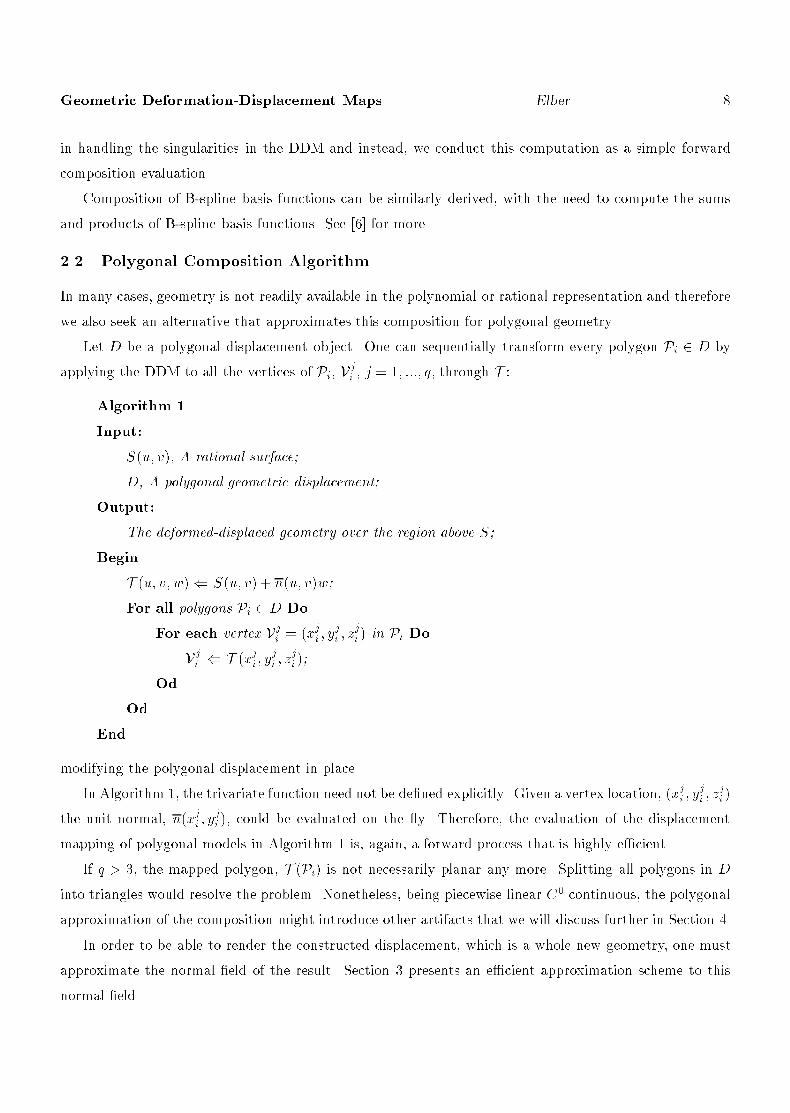
2.2 Polygonal Composition Algorithm
In many cases, geometry is not readily available in the polynomial or rational representation and therefore
we also seek an alternative that approximates this composition for polygonal geometry.
Let D be a polygonal displacement object. One can sequentially transform every polygon Pi 2 D by
applying the DDM to all the vertices of Pi, Vji , j = 1; :::; q, through T :
Algorithm 1
Input:
S(u; v), A rational surface;
D, A polygonal geometric displacement;
Output:
The deformed-displaced geometry over the region above S;
Begin
T (u; v; w)( S(u; v) + n(u; v)w;
For all polygons Pi 2 D Do
For each vertex Vji = (xji ; y
ji ; z
ji ) in Pi Do
Vji ( T (xji ; yji ; z
ji );
Od
Od
End
modifying the polygonal displacement in place.
In Algorithm 1, the trivariate function need not be de�ned explicitly. Given a vertex location, (xji ; y
ji ; z
ji )
the unit normal, n(xji ; y
ji ), could be evaluated on the y. Therefore, the evaluation of the displacement
mapping of polygonal models in Algorithm 1 is, again, a forward process that is highly e�cient.
If q > 3, the mapped polygon, T (Pi) is not necessarily planar any more. Splitting all polygons in D
into triangles would resolve the problem. Nonetheless, being piecewise linear C0continuous, the polygonal
approximation of the composition might introduce other artifacts that we will discuss further in Section 4.
In order to be able to render the constructed displacement, which is a whole new geometry, one must
approximate the normal �eld of the result. Section 3 presents an e�cient approximation scheme to this
normal �eld.

Geometric Deformation-Displacement Maps Elber 9
3 E�cient Normal Estimation
Given a geometry that undergoes some transformation T , the normal at some vertex could be either
mapped directly using T or be approximated as the average of the normals of the mapped polygons
sharing this vertex. While clearly feasible, such normal averaging could be time consuming. Hence, we
seek the conditions under which an approximation could be derived from the original normals by mapping
these normals directly through T .
A mapping T is called conformal [5] if it preserves angles. Speci�cally a conformal mapping will preserve
the orthogonality between the normal vector and the tangent plane of the surface. While, for example,
a rigid motion is clearly conformal, a general trivariate function is hardly so. Nonetheless, the type of
trivariate functions presented (See Equation (3)) do preserve angles to a certain extent and hence could
be considered conformal under some conditions.
Let P0 = D(r0; t0) be a point in the displacement map, P0 = (u0; v0; w0) and let N0 = (nu0 ; nv0; n
w0 )
be the normal of the displacement surface, D, at P0. Recall that B is the parametric domain (u; v; w)
of trivariate T (u; v; w) = S(u; v) + n(u; v)w. Let Vu, Vv, and Vw be three unit vectors in the parametric
domain B along u, v, and w, respectively. Vu, Vv, and Vw form an orthonormal basis that spans B and
hence the following holds:
N0 = (hN0; VuiVu + hN0; VviVv + hN0; VwiVw)
= nu0Vu + nv0Vv + nw0 Vw;
where h�; �i denotes the inner product of the vectors.
At P0, the three vectors of Vu, Vv, and Vw are mapped by T to the three vectors of
@T (u; v; w)
@u
����(u=u0;v=v0;w=w0)
=@S(u0; v0)
@u+@n(u0; v0)
@uw0;
@T (u; v; w)
@v
����(u=u0;v=v0;w=w0)
=@S(u0; v0)
@v+@n(u0; v0)
@vw0;
@T (u; v; w)
@w
����(u=u0;v=v0;w=w0)
= n(u0; v0); (8)
respectively. Then, normal N0 at P0 is mapped by T (u; v; w) into
T (N0) = hN0; Vui@T
@u
+ hN0; Vvi@T
@v
+ hN0; Vwi@T
@w
����(u=u0;v=v0;w=w0)
= nu0
�@S(u0; v0)
@u+@n(u0; v0)
@uw0
�
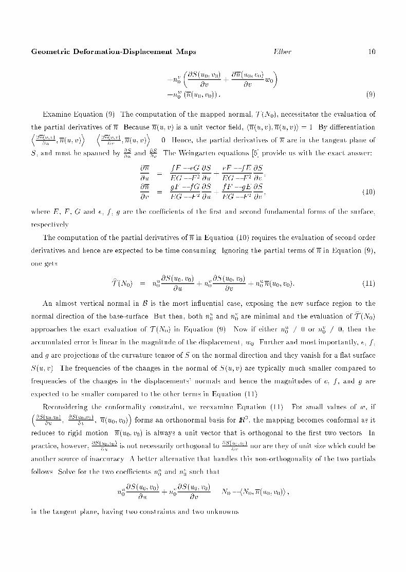
Geometric Deformation-Displacement Maps Elber 10
+nv0
�@S(u0; v0)
@v+@n(u0; v0)
@vw0
�+nw0 (n(u0; v0)) : (9)
Examine Equation (9). The computation of the mapped normal, T (N0), necessitates the evaluation of
the partial derivatives of n. Because n(u; v) is a unit vector �eld, hn(u; v); n(u; v)i = 1. By di�erentiationD@n(u;v)
@u; n(u; v)
E=
D@n(u;v)
@v; n(u; v)
E= 0. Hence, the partial derivatives of n are in the tangent plane of
S, and must be spanned by@S@u
and@S@v. The Weingarten equations [5] provide us with the exact answer:
@n
@u=
fF � eG
EG� F 2
@S
@u+eF � fE
EG� F 2
@S
@v;
@n
@v=
gF � fG
EG� F 2
@S
@u+fF � gE
EG� F 2
@S
@v; (10)
where E, F , G and e, f , g are the coe�cients of the �rst and second fundamental forms of the surface,
respectively.
The computation of the partial derivatives of n in Equation (10) requires the evaluation of second order
derivatives and hence are expected to be time consuming. Ignoring the partial terms of n in Equation (9),
one gets
bT (N0) = nu0@S(u0; v0)
@u+ nv0
@S(u0; v0)
@v+ nw0 n(u0; v0): (11)
An almost vertical normal in B is the most in uential case, exposing the new surface region to the
normal direction of the base-surface. But then, both nu0 and nv0 are minimal and the evaluation ofbT (N0)
approaches the exact evaluation of T (N0) in Equation (9). Now if either nu0 6= 0 or nv0 6= 0, then the
accumulated error is linear in the magnitude of the displacement, w0. Further and most importantly, e, f ,
and g are projections of the curvature tensor of S on the normal direction and they vanish for a at surface
S(u; v). The frequencies of the changes in the normal of S(u; v) are typically much smaller compared to
frequencies of the changes in the displacements' normals and hence the magnitudes of e, f , and g are
expected to be smaller compared to the other terms in Equation (11).
Reconsidering the conformality constraint, we reexamine Equation (11). For small values of w, if�@S(u0;v0)
@u;@S(u0;v0)
@v; n(u0; v0)
�forms an orthonormal basis for IR
3, the mapping becomes conformal as it
reduces to rigid motion. n(u0; v0) is always a unit vector that is orthogonal to the �rst two vectors. In
practice, however,@S(u0;v0)
@uis not necessarily orthogonal to
@S(u0;v0)
@vnor are they of unit size which could be
another source of inaccuracy. A better alternative that handles this non-orthogonality of the two partials
follows. Solve for the two coe�cients nu0 and nv0 such that
nu0@S(u0; v0)
@u+ nv0
@S(u0; v0)
@v= N0 � hN0; n(u0; v0)i ;
in the tangent plane, having two constraints and two unknowns.

Geometric Deformation-Displacement Maps Elber 11
(a) (b) (c) (d)
Figure 3: Examples of few tiles that are used as geometric displacements in this work. In (a) and (b), a
thorn and a square covering tiles are shown. In (c) and (d), scales and fur casual tiles are presented.
In order to be able to estimate the normal �eld of the displacement, asbT (N0) in Equation (11), one
needs not only the surface normal at each vertex Vji but also the two partial derivatives of the surface, data
that is not typically provided by contemporary rendering tools, yet, in most cases, is readily available. In
other words, we are in need of a continuous parameterization of the surface of the object, a parameterization
that is as close to an Isometry [5] as possible to the unit square parametric domain. If the input data
is formed out of parametric surfaces, the original parameterization of the base-surfaces could typically be
employed, providing the trihedra of vectors
�@S@u; @S@v; n�per vertex, Vji . In recent years, the derivation of
parameterizations for polygonal meshes has been rigorously investigated [9, 24, 25] for texture mapping
purposes as well as others. In [25], the surface tangents are already structured into each vertex. The end
results of these parameterization could then be used directly to de�ne this trihedra for polygonal meshes.
The use ofbT (N0) to approximate the normal �eld was found to be adequate in all examples we created,
as we will be demonstrated in Section 4.
4 Examples and Extensions
All the examples presented in the section were created using an implementation that is based on the
IRIT [14] solid modeling environment, developed at the Technion. All the ray traced images presented in
this work were created using the POVRAY [20] ray tracer.
Figure 3 shows few examples of geometric tiles that are used in the section. Shown is a thorn tile
(Figure 3 (a)), a three-dimensional square tile (Figure 3 (b)), scales' tile (Figure 3 (c)), and a fur tile
(Figure 3 (d)).
In Figure 4, the Utah teapot is shown with a covering displacement map, in the form of a chocolate
bar. The tile used is shown in Figure 3 (b). When the geometry of the texture is tiled along the surface, it
should follow its curvature. Yet, when a polygonal displacement is mapped through T , the linear edges of
the polygons are always mapped into linear edges, regardless of the degree of the trivariate. To alleviate
this artifact, one can subdivide large polygons in the displacement to smaller ones. In Figure 5 (a), one
can see one sample of this potential problem when closely inspecting the tip of the teapot's spout. The
top at region of the chocolate tile in Figure 3 (b) is represented as one polygon in Figure 5 (a) and is

Geometric Deformation-Displacement Maps Elber 12
Figure 4: The Utah teapot with a covering DDM and tiles in the shape of chocolate bars. See tile in
Figure 3 (b).
(a) (b)
Figure 5: Both (a) and (b) employ the tile seen in Figure 3 (b) texturing the spout of the teapot shown in
Figure 4. (a) employs a single polygon for the top at domain of the tile whereas in (b) this at domain
is subdivided into small polygons giving a better looking, smoother result. Note the self-shadows that are
clearly visible.
subdivided into several polygons in Figure 5 (b). Clearly, the latter has a superior look. The question of
a su�cient subdivision level of large polygons is beyond the scope of this work. This exact problem exists
in every FFD that is applied to polygonal data and while we are aware of no prior work on this subject,
it is a general FFD related concern.
Another classic example of this type of texturing is the simulation of scales. Figure 6 shows an example
of geometric scales (see tile in Figure 3 (c)) over the surfaces of the Utah teapot. Note that while the scales
do not form a covering texture, they do, in practice, establish an almost complete cover of the surface area.

Geometric Deformation-Displacement Maps Elber 13
Figure 6: The Utah teapot with scales' texture style. See tile in Figure 3 (c).
While the texture tile is supposed to be de�ned over a (unit) square domain, the geometry in Figure 3 (c)
exceeds that domain. This geometric extension is treated with ease, by continuously handling the proper
extension beyond the assigned square tile domain and into the neighboring tile(s). It is this behavior of
the tile that allows us to de�ne the scales and make them overlap. Moreover, if the base-surface, S(u; v),
is periodic along either u or v this geometric extension could be propagated across the boundary onto the
other side of the base-surface. This is the case for one of the two parametric directions on all four surfaces
of the Utah teapot.
In Figure 7, the light chess pieces are covered by a thorn geometric texture tile shown in Figure 3 (a)
while the dark pieces use the casual scales seen in Figure 3 (c) that cover the pieces almost completely.
The fact that the texture is a regular geometry allows us to preserve the geometric context and modify the
attributes of the texture geometry at will. The light pieces have thorns that are color-modulated with a
low frequency volumetric noise function, globally and continuously over each chess piece. In contrast, the
texture of the dark pieces is formed out of two types of scales, each with di�erent color and color-modulation
functions.
Casual texture could be fed from almost any source of geometry. In Figure 8, the Utah teapot is
recursively and smoothly tiled over all its four surfaces. Two levels of recursion are presented.
The trivariate functions that were de�ned until now (see Equation (2)) assumed that the volume above
the surface is linearly parameterized along w and in the direction of the normal to (the tangent plane of)

Geometric Deformation-Displacement Maps Elber 14
Figure 7: A chess set with a covering displacement map in the shapes of thorns for the light pieces and a
casual displacement map of scales for the dark pieces (about 1,100,000 polygons).
Figure 8: The Utah teapot serving as a casual texture for itself. Two levels of recursions are presented.

Geometric Deformation-Displacement Maps Elber 15
(a) (b) (c)
Figure 9: The Utah teapot with casual fur textures. In (a), the fur is oriented along the normals of the
surfaces (about 600,000 polygons). In (b) and (c), gravity and wind bias are added to the created fur
texture, pulling the hair downwards and sidewards, respectively. A zoom on the region of the spout is
shown in (b) and (c). The tile itself can be seen in Figure 3 (d).
the surface. Clearly, this need not be the case. For example, consider the trivariate function above the
surface S that is de�ned as
T (u; v; w) = S(u; v)+ n(u; v)w+ wk; w > 0: (12)
is some prescribed attraction vector having its e�ect controlled to the k'th power with respect to w.
The in uence of increases as we move away from the surface. One intuitive view of this e�ect is gravity
(vertical ) or wind in the direction of . All the volume above the surface S will be attracted to the
direction of , bending all the geometry of the displacement with it.
Figure 9 shows several examples of simulation of fur over the Utah teapot, with and without the
attraction vector. The basic casual fur geometric tile that is used in Figure 9 can be seen in Figure 3 (d).
A continuous interpolation between two geometric displacement tiles could o�er a smooth transition in
time between two textures. For example, by smoothly interpolating two types of thorns or even between a
thorn tile and a ower, one can create a smooth animation of metamorphed texture. This simple extension
has a clear power over the traditional, image based, displacement mapping where the geometric context
is lost. Due to the generality of the presented DDM technique, any kind of geometric metamorphosis
technique may be employed between the source and target tiles to create such interpolation sequences.
Figure 10 shows one such example, presenting few snapshots from an animation of geometric displacement
tiles that are metamorphed between a thorn and a ower.
Arbitrary complex shapes could be warped and glued to the surface. One example of such a complex
shape is seen in Figures 11, successfully exploiting models of high complexity and �tting them along the

Geometric Deformation-Displacement Maps Elber 16
Figure 10: Because any geometry could be warped along the base-surface and texture it, one can employ
any available metamorphosis technique to blend between two geometric texture tiles. Shown are a few
snapshots from such a metamorphosis animated sequence presenting a thorn changing to a ower.
shape of a glass. Attempts to glue geometry on given surfaces are known, such as the recent example
of [13], mostly toward decorative purposes. In [13] a primary-orientation pair of curves is used to guide
the warping function along the base surface, an easier to maintain approach compared to the approach
presented herein. Yet, continuity conditions can not be guaranteed and the behaviour above the surface is
not easily controlled, resulting in less general scheme.
5 Conclusions and Future Work
This work generalizes the idea of displacement maps, extending this notion from explicit displacement maps
to arbitrary geometric and/or parametric forms. The ability to de�ne a continuous map from a subset of
IR3to the IR
3region above the surface is powerful and allows the precise placement of geometric texture
elements near each other while neatly and smoothly following the curvature of the surface. The proposed
DDM scheme allows both deformations and displacements to be applied to the constructed texture, where

Geometric Deformation-Displacement Maps Elber 17
Figure 11: Six Happy Buddhas from the Stanford 3D Scanning Repository [22] are warped around a golden
glass, only to serve as its base.
the displacement's shape is mainly governed by D and the deformation function is fully prescribed by T .
Finally, we have also presented an e�cient scheme to approximate the normals of this displaced geometry.
The method presented generates large amounts of polygonal data. Having a representation that ge-
ometrically creates highly detailed texture, methods should be sought to either compress or reduce this
excessive amount of data, in the order of hundreds of thousands of polygons. The fact that the DDM
is none linear, makes it more di�cult to compute its inverse and remap the traced rays instead of the
geometry as is done, for example, in [15].
The basic trivariate function expressed in Equation (2) implicitly derives the o�set function of the input
surface. This close connection to the o�set operation deserves some further investigation.
Freeform parametric B�ezier and B-spline surfaces are rarely isometric. This could results in artifacts
in the mapped texture that scale D to di�erent sizes in di�erent surface locations. Similarly, improper
subdivision of the deformed and displaced texture could yield poor results as can be seen in Figure 5.
Methods to �gure out the proper and necessary subdivision level of D when it is represented as a polygonal
geometry must be derived, a result that will also directly re ect to regular FFDs. In Figures 4 and 6 the

Geometric Deformation-Displacement Maps Elber 18
chocolate bars and the scales vary in size. While it is impossible to guarantee a �xed tile size in Euclidean
space, one could alleviate these distortions. For example, the scales at the top region of the body in
Figure 6 are much smaller. Due to a slower v speed at that region of the body surface, the scales are
smaller. Clearly, a simple reparametrization of this surface could resolve this speci�c problem.
The representation of the displacement above a surface as a trivariate warping operation brings together,
under a uni�ed umbrella a variety of surface texturing techniques such as hair, fur, and scales simulations,
as well as the displacement mapping method. Furthermore, traditional displacement mapping was shown
to be a restricted case of the object warping technique using trivariate functions. By taking advantage of
the full capabilities of these warping operators, we were able to elevate the capabilities of displacement
maps onto a new level.
The presented approach can also serve as the mathematical framework for modeling of details. Once
the general shape is de�ned, one can employ the presented approach as a post-process that allows the user
to interact with di�erent types of surface details, drawing from a library of texture geometry, whether
casual or covering.
6 Acknowledgment
The model of the Happy Buddha used as displacement map in Figures 11 has been provided courtesy of
The Stanford 3D Scanning Repository [22].
References
[1] J. F. Blinn. Simulation of Wrinkled Surfaces ACM SIGGRAPH 78 Conference Proceedings, Vol 12,
No. 3, pp 286{292, Aug. 1978.
[2] E. Cohen, R. F. Riesenfeld, and G. Elber. Geometric Modeling with Splines: An Introduction. A. K.
Peters, Natick Massachusetts, 2001.
[3] R. L. Cook. Shade trees ACM SIGGRAPH 84 Conference Proceedings, Vol 18, pp 223{231, Jul. 1984.
[4] S. Coquillart. Extended free-form deformations: A sculpting tool for 3D geometric modeling. ACM
SIGGRAPH 90 Conference Proceedings, pp 187-196, Aug. 1990.
[5] M. do Carmo. Di�erential Geometry of Curves and Surfaces. Prentice-Hall, 1976.
[6] G. Elber. Symbolic and numeric computation in curve interrogation. Computer Graphics Forum, 14
(1995), pp. 25 { 34.

Geometric Deformation-Displacement Maps Elber 19
[7] G. Elber and M. S. Kim. Geometric Constraint Solver using Multivariate Rational Spline Functions.
The Sixth ACM/IEEE Symposium on Solid Modeling and Applications, Ann Arbor, Michigan, pp
1-10, June 2001.
[8] G. Farin. Curves and Surfaces for Computer Aided Geometric Design, a Practical Guide., Academic
Press, Inc., fourth ed., 1997.
[9] M. S. Floater. Parameterization and Smooth Approximation of Surface Triangulation. Computer
Aided Geometric Design, Vol 14, No. 3, pp 231-250, 1997.
[10] K. Fleischer, D. Laidlaw, B. Currin, and A. Barr. Cellular Texture Generation. ACM SIGGRAPH 95
Conference Proceedings, pp 239{248, Aug. 1995.
[11] J. D. Foley, A. Van Dam, S. K. Feiner, and J. F. Hughes. Fundamentals of Interactive Computer
Graphics. Addison-Wesley Publishing Company, second edition, 1990.
[12] J. E. Gain and N. A. Dodgson. Preventing Self-Intersection under Free-Form Deformation. IEEE
Transaction on Visualization and Computer Graphics, Vol 7, No. 4, Oct.-Dec. 2001.
[13] K.C.Hui. Freefrom design using axis curve-pairs. Computer Aided Design, Vol 34, No. 8, pp 583-596,
2002.
[14] IRIT 8.0 User's Manual. The Technion|IIT, Haifa, Israel, 2000. Available at
http://www.cs.technion.ac.il/~irit.
[15] J. T. Kajiya and T. L. Kay. Rendering Fur with Three Dimensional Textures. ACM SIGGRAPH
89 Conference Proceedings, pp 271-280, Jul. 1989.
[16] K. Kim and G. Elber. New Approaches to Freeform Surface Fillets. The Journal of Visualization
and Computer Animation, Vol 8, No 2, pp 69-80, 1997. Also the third Paci�c Graphics Conference on
Computer Graphics and Applications, Seoul, Korea, pp 348-360, August 1995.
[17] M. Legakis, J. Dorsey, and S. Gortler. Feature Based Cellular Texturing for Architectural Models.
ACM SIGGRAPH 2001 Conference Proceedings, pp 309-316, Aug. 2001.
[18] R. MacCracken and A. P. Rockwood. Free-Form Deformations with Lattices of Arbitrary Topology.
ACM SIGGRAPH 96 Conference Proceedings, pp 181{188, Aug. 1996.
[19] F. Neyret. Modeling, Animating, and Rendering Complex Scenes using Volumetric textures. IEEE
Transaction on Visualization and Computer Graphics, Vol 4, No. 1, Jan 1998.

Geometric Deformation-Displacement Maps Elber 20
[20] The POVRAY ray tracer. www.povray.org.
[21] T. W. Sederberg and S. R. Parry. Free-Form Deformation of Solid Geometric Models ACM SIG-
GRAPH 86 Conference Proceedings, Vol 20, pp 151-160, Aug. 1986.
[22] The Stanford 3D Scanning Repository, http://www-graphics.stanford.edu/data/3Dscanrep.
[23] G. Turk. Generating Textures for Arbitrary Surfaces using Reaction-Di�usion. ACM SIGGRAPH 91
Conference Proceedings, pp 289{298, Jul. 1991.
[24] G. Turk. Texture Synthesis on Surfaces. ACM SIGGRAPH 2001 Conference Proceedings, pp 347-354,
Aug. 2001.
[25] L. Y. Wei and M. Levoy. Texture Synthesis over Arbitrary Manifold Surfaces. ACM SIGGRAPH 2001
Conference Proceedings, pp 355-360, Aug. 2001.
[26] A. Witkin and M. Kass. Reaction-Di�usion Textures. ACM SIGGRAPH 91 Conference Proceedings,
pp 299{308, Jul. 1991.