1

David SimpsonThemis Inc.

dsimpson@themisinc.com

SQL Optimization & Access Paths: What’s Old & New

Part 2

© 2008 Themis, Inc. All rights reserved.

David Simpson is currently a Senior Technical Advisor at Themis Inc. He teaches courses on SQL, Application Programming, DB2 Administration as well as performance and tuning. He has supported transactional systems that use DB2 for z/OS databases in excess of 10 terabytes. David has worked with DB2 for 14 years as an application programmer, DBA and technical instructor. David is a certified DB2 DBA on both z/OS and LUW. David was voted Best User Speaker and Best Overall Speaker at IDUG North America 2006. He was also voted Best User Speaker at IDUG Europe 2006.

2

Disclaimer

In other words….IT still DEPENDS!

The content of this presentation reflects my personal experience and is a product of the systems and applications I have worked with. Your results may vary. My results may or may not be typical.

“Themis makes no representation, warranties or guarantees whatsoever in relationship to the information contained in this presentation. This presentation is provided solely to share information with the audience relative to the subject matter contained in the presentation and is not intended by the presenter or Themis to be relied upon by the audience of this presentation.”

3

REQUEST RESPONSE

DB2STAGE 2

(Non-Sargable)RDS

DM

BM

STAGE 1(Sargable)

IndexableSTAGE 1

Index Access Data Access

Predicate Processing

DB2 is modular in structure. Understanding the structure of DB2 can help you evaluate SQL efficiencies and anticipate what the most likely access method DB2 will choose to satisfy SQL requests. The following subcomponents are part of the Database Services Address Space (DBAS).

RELATIONAL DATA SYSTEM (RDS)♦ Responsible for providing all the relational operators♦ Predicts when requests can be passed as search arguments called "Sargable Predicates"♦ Passes search arguments to Data Manager

DATA MANAGER (DM)♦ Looks at RDS request and determines what page is required. Issues GETPAGE request to Buffer Manager.♦ Transforms page data into row and column format for RDS.

Stage 1 and Stage 2 PredicatesRows retrieved for a query go through two stages of processing.♦ Stage 1 predicates (sometimes called "sargable") can be applied during the first stage.♦ Stage 2 predicates (sometimes called "nonsargable" or "residual") cannot be applied until the second stage.

4

Is My Predicate Stage 1?

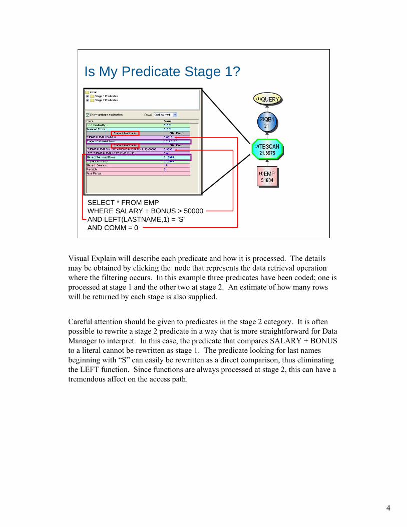
SELECT * FROM EMPWHERE SALARY + BONUS > 50000AND LEFT(LASTNAME,1) = 'S'AND COMM = 0

Visual Explain will describe each predicate and how it is processed. The details may be obtained by clicking the node that represents the data retrieval operation where the filtering occurs. In this example three predicates have been coded; one is processed at stage 1 and the other two at stage 2. An estimate of how many rows will be returned by each stage is also supplied.

Careful attention should be given to predicates in the stage 2 category. It is often possible to rewrite a stage 2 predicate in a way that is more straightforward for Data Manager to interpret. In this case, the predicate that compares SALARY + BONUS to a literal cannot be rewritten as stage 1. The predicate looking for last names beginning with “S” can easily be rewritten as a direct comparison, thus eliminating the LEFT function. Since functions are always processed at stage 2, this can have a tremendous affect on the access path.

5

Converting a Predicate to Stage 1

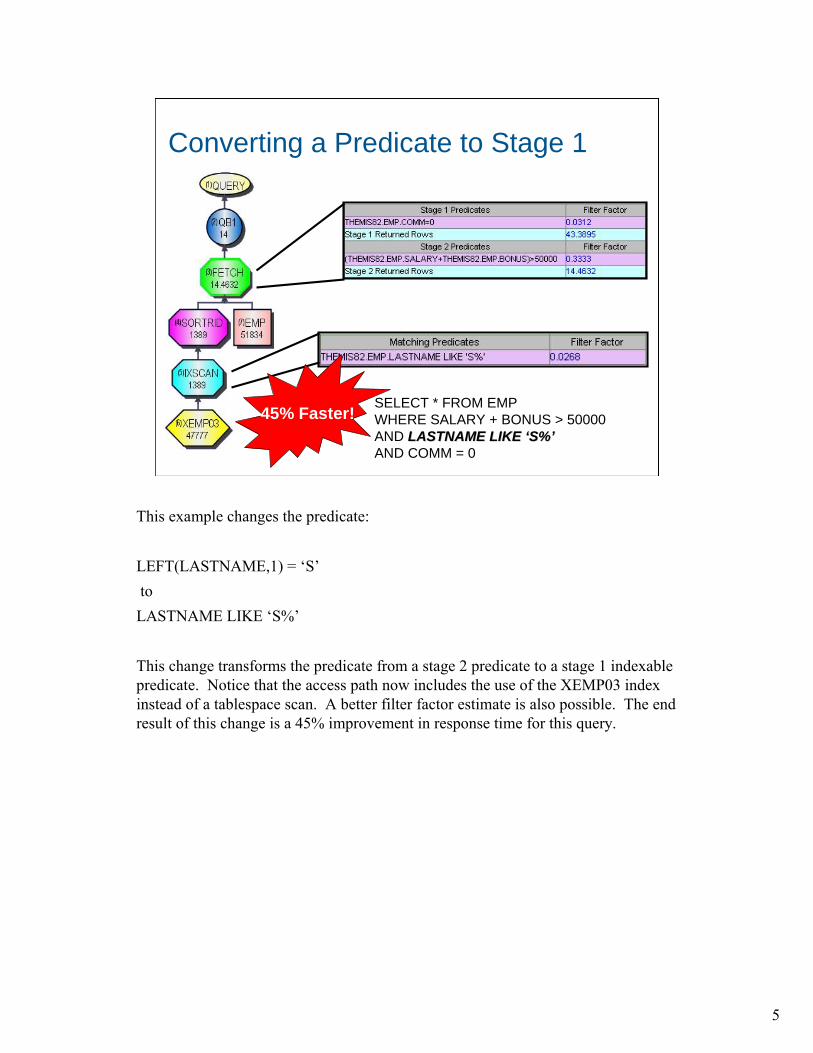
SELECT * FROM EMPWHERE SALARY + BONUS > 50000AND LASTNAME LIKE LASTNAME LIKE ‘‘S%S%’’AND COMM = 0

45% Faster!

This example changes the predicate:

LEFT(LASTNAME,1) = ‘S’to LASTNAME LIKE ‘S%’

This change transforms the predicate from a stage 2 predicate to a stage 1 indexablepredicate. Notice that the access path now includes the use of the XEMP03 index instead of a tablespace scan. A better filter factor estimate is also possible. The end result of this change is a 45% improvement in response time for this query.

6

Catalog Statistics and Filter Factors

…………Q…………X…………Y…………Q…………Q…………Z…………Q…………W…………Q

C5C4C3C2C1

DB2 determines 5 distinct values for column C1.

Filter Factor

Table T1

For the predicate C1 = ‘Z’; DB2 would estimate that 1/5 of the rows would qualify.The filter factor would be .20.

Food For Thought: Is this filter factor accurate?

The percentage of rows that qualify for any given predicate.

The filter factor of a predicate is a number between 0 and 1 that estimates the proportion of rows in a table for which the predicate is true. Those rows are said to qualify by that predicate.

Suppose that DB2 can determine that column C1 of table T1 contains only five distinct values: Q, W, X, Y, and Z. In the absence of other information, DB2 estimates that one-fifth of the rows have the value ‘Q’ in column C1. Then the predicate C1='Q' has the filter factor 0.2 for table T1.

DB2 calculates filter factors for predicates during access path selection using the statistics available in the Catalog. It is these filter factors that help determine the least costly access path for any given SQL statement.

7

Calculating Filter Factors• Default Filter Factors (no stats)

• Uniform Distribution Filter Factor (COLCARDF is populated)

• Non-uniform Distribution Filter Factor (SYSIBM.SYSCOLDIST is populated)

• Interpolation Formulas (if HI2KEY AND LOW2KEY are populated)

How a filter factor is determined depends on the level of detail in the statistics gathered and how much information is available in the SQL to be optimized. If no statistics have been gathered for a given column then defaults are used to make the determination. If basic column level statistics exist for the referenced column then DB2 knows the approximate number of values that exist for that column in the data (COLCARDF). The optimizer assumes an even distribution of values across the column and calculates the filter factor accordingly. If frequency statistics have also been gathered for the referenced column AND literals are used in the SQL statement then the optimizer can make an even better estimate because it is aware of potential uneven distribution of the data. For range predicates interpolation formulas may be used to estimate what percentage of the values will qualify.

8

Factors for Uniform Distributions

Interpolation formulaCOL Op2 literal

Note:Op1 is < or <=, and the literal is not a host variable.Op2 is > or >=, and the literal is not a host variable.Literal is any constant value that is known at bind time.

Interpolation formulaCOL BETWEEN literal1 and literal2

Interpolation formulaCOL LIKE literal

Interpolation formulaCOL Op1 literal

Number of literals/COLCARDF COL IN (literal list)

1/COLCARDFCOL IS NULL

1/COLCARDFCOL = literal

FILTER FACTORPEDICATE TYPE

The table on this page illustrates uniform distribution filter factors for different types of predicates. If column level statistics have been gathered, then the value of COLCARDF in SYSIBM.SYSCOLUMNS will be populated with the approximate number of unique values for that column. If no additional statistics are available, the optimizer assumes uniform distribution of the data across these values.

DB2 uses these filter factor values when:•There is a positive value in column COLCARDF of catalog table SYSIBM.SYSCOLUMNS for the column. •There are no additional statistics for the column in SYSIBM.SYSCOLDIST.

Again, consider the following example. SELECT . . . . FROM T1 WHERE C1 = ‘D’;

If ‘D’ is one of only five distinct values in column C1, running RUNSTATS utility would be set SYSIBM.SYSCOLCARDF for C1 to the number 5. Under these circumstances, DB2 is able to use the uniform distribution filter factor for this predicate. The uniform distribution filter factor for a predicate COL = literal is 1/ COLCARDF, thus 1/5 (0.20). The accurate filter factor indicates that a larger number of rows would qualify.DB2’s ability to use actual statistics to determine filter factors will lead to more effective and efficient access paths.

9

Non Uniform Distribution• Frequently occurring default

values or uneven distribution of values for a column often cause optimizer issues

• Additional Statistics may be gathered to give the optimizer additional information

• Stats for indexed columns only in V7, all columns in V8

Data skew is one of the greatest challenges for the optimizer when determining an accurate filter factor. Unless frequency statistics are gathered, the optimizer assumes even distribution across the values for a column. If there are outliers that are statistically significant the optimizer could be led to select a bad access path.

In Version 7, frequency statistics could be gathered on any index column or combination of indexed columns. In V8, this capability has been extended to all columns. Consider requesting these statistics for any column or column groups that are frequently used for filtering in SQL statements, particularly data skew exists for that column or column group. The data skew statistics are stored in the catalog table SYSCOLDIST.

10

Non Uniform Distribution

From SYSCOLDIST

These statistics are displayed in Visual Explain in the “Coldist” folder. In the example shown, the top 4 values for the JOB column have been collected via the RUNSTATS utility. The decimal value shown is expressed as a percentage of the rows that contain that value. According to these statistics, the value of “ASSEMBLY” occurs on over 99% of the rows, so the data skew is evident.

11

Non Uniform Distribution

From SYSCOLDIST

SELECT *FROM EMP

WHERE JOB = ‘MANAGER’

FF = .0020256974

If one of the collected values is requested in the WHERE clause of a query, the filter factor is lifted directly from SYSCOLDIST rather than computed or defaulted.

12

Non Uniform Distribution

SELECT *FROM EMP

WHERE JOB = ‘VP’FF = .000000001 ???

Even if an SQL statement is submitted requesting a value not stored in SYSCOLDIST, the extra statistics are still of some value. In this example a value of “VP” is requested which is not one of the top 4 values collected. Even distribution would compute a filter factor of 1/9 (.111). Since the values that were collected account for over 99% of the data, the optimizer knows that the remaining 5 values must all occur on a very small fraction of the rows. The resulting filter factor is very small.

13

Explain With Basic Column Stats

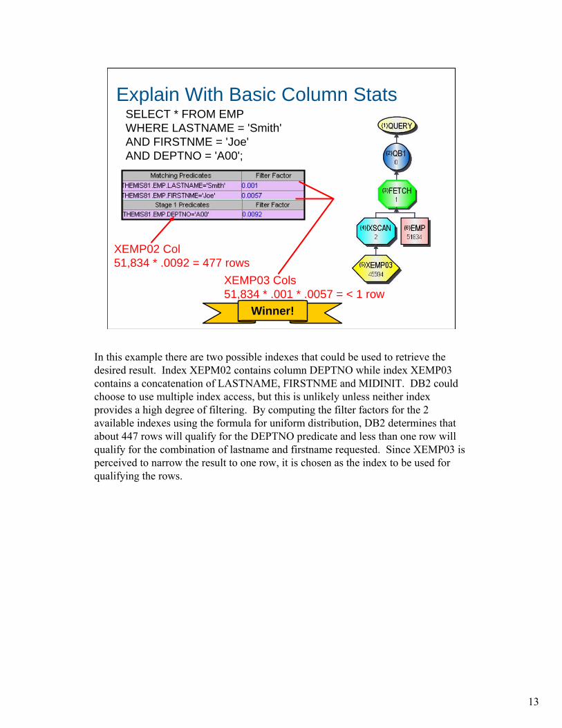
XEMP03 Cols51,834 * .001 * .0057 = < 1 row

XEMP02 Col51,834 * .0092 = 477 rows

Winner!

SELECT * FROM EMPWHERE LASTNAME = 'Smith'AND FIRSTNME = 'Joe'AND DEPTNO = 'A00';

In this example there are two possible indexes that could be used to retrieve the desired result. Index XEPM02 contains column DEPTNO while index XEMP03 contains a concatenation of LASTNAME, FIRSTNME and MIDINIT. DB2 could choose to use multiple index access, but this is unlikely unless neither index provides a high degree of filtering. By computing the filter factors for the 2 available indexes using the formula for uniform distribution, DB2 determines that about 447 rows will qualify for the DEPTNO predicate and less than one row will qualify for the combination of lastname and firstname requested. Since XEMP03 is perceived to narrow the result to one row, it is chosen as the index to be used for qualifying the rows.

14

Compare with Reality

SELECT COUNT(*)FROM EMPWHERE LASTNAME = 'Smith'AND FIRSTNME = 'Joe';

1,289 rows

(DB2 est. <1)

SELECT COUNT(*)FROM EMPWHERE DEPTNO = 'A00';

4 rows

(DB2 est. 477)

If this query is not performing optimally, it may be useful to compare the filter factors presented in Visual Explain with actual row counts on the tables involved. In this case, the optimizer’s estimate of 1 row for index XEMP03 was incorrect (1289 rows actually exist). The estimate for XEMP02 of 477 qualifying rows was also incorrect (actual count was only 4).

In this case a poor filter factor estimate led to the wrong index being selected.

15

Additional Statistics

RUNSTATS INDEX (THEMIS82.XEMP02) KEYCARD FREQVAL NUMCOLS 1 COUNT 5 BOTH

RUNSTATS INDEX (THEMIS82.XEMP03) KEYCARD FREQVAL NUMCOLS 2 COUNT 5 MOST

A00 has far fewer rows than the average dept

Joe Smith has far more rows than the average name combination

Uneven distribution of data in this table is the reason for the poor filter factor estimates. In this case department A00 has far fewer occurrences than the average department. Joe Smith also occurred far more frequently than the average name combination. Additional index statistics may be gathered to inform the optimizer of the statistical outliers. In the first control card, the runstats utility is being requested to capture both the 5 most frequently occurring values and the 5 least frequently occurring values for DEPTNO and store these values in SYSCOLDIST. The second control card is requesting the top 5 combinations for the first two columns of XEMP03 (LASTNAME and FIRSTNME).

16

Frequency Stats

Once these statistics have been gathered they may be viewed using Visual Explain in the Coldist folder for the column statistics. The appropriate filter factor for department A00 is .000077 rather than .0092 as calculated using uniform distribution rules. This leads DB2 to estimate that about 4 rows will qualify for this predicate, which is exactly what the actual count revealed.

17

Result of Adding Frequency Stats

With the additional statistics in place, the optimizer chooses XEMP02 to accomplish the filtering instead of XEMP03 resulting in better performance. More rows are eliminated from consideration earlier in the process using this access path.

18

Join OrderSELECT *FROM EMP E, PROJ PWHERE E.EMPNO = P.EMPNOAND E.COMM = 0AND P.PRSTAFF > 3

A similar problem can occur when joining tables together even when the predicates involved are not indexed. In this example the EMP table is being joined to the PROJ table. Local predicates exist on both tables, so DB2 must make what appears to be a narrow decision on which table should be accessed first.

19

Comparing Estimates with Reality

SELECT COUNT(*)FROM EMPWHERE COMM = 0;

51,803 rows

(DB2 est. 1,620)

SELECT COUNT(*)FROM PROJWHERE PRSTAFF > 3;

14,598 rows

(DB2 est. 50,242 * .2906 = 14,600)

# Rows on PROJ

Filter Factor

The optimizer calculates that 1620 rows will qualify in the EMP table using formulas for uniform distribution. Actual counts reveal that 51,803 rows actually exist that meet the requested condition. Zero appears to be a default value for COMM that occurs much more often than any other value. This is a fairly common condition. Many columns have default or null values that occur much more often than anything else.

Prior to Version 8, there was no way to provide additional statistics with the runstats utility that would help this situation for non-indexed columns. Values could be manually added to SYSCOLDIST (sometimes with the help of the DSTATS program), but not collected by DB2.

20

Additional Statistics

RUNSTATS TABLESPACE THEMIS82.TS00EMP TABLE(THEMIS82.EMP) COLUMN(COMM)COLGROUP(COMM) FREQVAL COUNT 1SORTDEVT SYSDA SORTNUM 4

COMM = 0 has far more rows than the average value

Introduced in V8 for non-indexed

columns

The syntax presented here will gather column level statistics for the COMM column and also gather the most frequently occurring value for COMM (COLCOUNT 1). Note that runstats must sort the data to obtain this information so sort parameters may need to be included in the syntax.

21

Join Order

SELECT *FROM EMP E, PROJ PWHERE E.EMPNO = P.EMPNOAND E.COMM = 0AND P.PRSTAFF > 3

When the additional statistics are provided, the optimizer understands the true nature of the data on the EMP table and chooses the PROJ table to be the first accessed since it provides much better filtering.

22

Range Predicates

SELECT LASTNAME, FIRSTNMEFROM EMPWHERE SALARY BETWEEN 20000 AND 50000;

SELECT LASTNAME, FIRSTNMEFROM EMPWHERE SALARY < 80000;

Range predicates are particularly susceptible to optimization problems since filter factors are difficult to compute accurately. If column level statistics are gathered, the optimizer will assume that data is evenly distributed between the values for LOW2KEY and HI2KEY on SYSCOLUMNS. If the data is not evenly distributed then the values for LOW2KEY and HI2KEY may need to be manually adjusted to achieve optimal performance for range predicates.

DB2 9 introduces histogram statistics that will give the optimizer a better picture of the distribution of values for range predicates.

23

Range Predicates

SELECT LASTNAME FROM EMPWHERE DEPTNO BETWEEN 'A00' AND 'Z99'

The range predicate in this example identifies nearly all the rows in the EMP table. Since LOW2KEY and HI2KEY are populated, the optimizer correctly calculates a filter factor of 1 and chooses a tablespace scan to retrieve the data.

24

Range Predicates

SELECT LASTNAME FROM EMPWHERE DEPTNO BETWEEN 'A00' AND ‘A01'

When the second value is changed so that a much narrower range of data is requested, the optimizer correctly lowers the filter factor and chooses an index to retrieve the few rows that are expected to qualify.

Problems may occur when the range encounters a “hot spot” in the data. Since the optimizer (in V8) always assumes even distribution, a narrow range on a “hot spot”could yield unexpected results.

25

Range Predicates

SELECT LASTNAME FROM EMPWHERE DEPTNO BETWEEN ‘P00’ AND ‘P99’

SELECT COUNT(*)FROM EMPWHERE DEPTNO BETWEEN 'P00' AND 'P99'

51,802 rows… 99% of the data

In this example, the wrong access path is chosen due to a hot spot. Over 99% of the data has a DEPTNO between P00 and P99, however the outliers cause the range determined by LOW2KEY and HI2KEY to appear much wider. In Version 8, it may be desirable to manually update LOW2KEY to ‘P00’ and HI2KEY to ‘P99’ to correct this problem.

This problem could also be solved using histogram statistics in DB2 9.

26

Host Variables

SELECT *FROM EMP E, PROJ PWHERE E.EMPNO = P.PROJNOAND E.COMM = ?AND P.PRSTAFF > ?

If host variables are used the optimizer cannot make effective use of frequency statistics to determine the access path. Uniform distribution of column values must be assumed in this situation. Whenever the access path has been determined with an unknown piece of information, a cost category of “B” will result.

27

REOPT Bind Parameter

REOPT (NONE) default

REOPT (ALWAYS) or REOPT(VARS)

REOPT (ONCE)

The REOPT bind parameter may be used to mitigate the problems associated with host variables. Packages or plans bound with REOPT(NONE) will always used the access path determined at bind time (for static SQL) or the access path from the dynamic statement cache (if present for dynamic SQL). This is the default behavior and should be the choice unless there is a good reason to select another option.

If the application is bound with REOPT(ALWAYS) or REOPT(VARS), access paths will always be re-evaluated at run time based on the values provided in host variables. This will happen each time a statement is executed. While this causes extra overhead at runtime, it may be prudent when host variables are causing the optimizer to choose a poor access path.

REOPT(ONCE) may be used for dynamic SQL to request an access path to be determined on its first occurrence based on the values in the host variables. Future invocations of the same statement will not be re-evaluated even if the host variable values change.

Since the REOPT parameter applies to all statements in a particular package or plan, it may be prudent to segregate statements that need this treatment from all other statements in an application into separate packages.

28

What’s in DB2 9 for Optimization

• Optimization Service Center

• Index on Expression – Can make complex expressions in a predicate Stage 1 Indexable

• Histogram Statistics

29

Reference

IBM Books

SC18-7426 DB2 UDB for OS/390 and z/OS SQL Reference V8

SC18-7413 DB2 UDB for OS/390 and z/OS Administration Guide V8

SC18-7427 DB2 UDB for OS/390 and z/OS Utility Guide and Reference V8

SG24-6079 DB2 UDB for z/OS Version 8: Everything You Ever Wanted to Know, ... and More

Previous IDUG Presentations

IDUG North America 2007 – More Ways to Challenge the DB2 z/OS Optimizer by Terry Purcell of IBM