SPSS 17 Technology Guide for Elementary Statistics - Cengage
26
SPSS 17 Technology Guide for Prepared by Nancy Pfenning University of Pittsburgh Melissa M. Sovak University of Pittsburgh Australia • Brazil • Japan • Korea • Mexico • Singapore • Spain • United Kingdom • United States Elementary Statistics: Looking at the Big Picture 1st EDITION Nancy Pfenning University of Pittsburgh
Transcript of SPSS 17 Technology Guide for Elementary Statistics - Cengage

SPSS 17 Technology Guide
for
Prepared by
Nancy Pfenning University of Pittsburgh
Melissa M. Sovak University of Pittsburgh
Australia • Brazil • Japan • Korea • Mexico • Singapore • Spain • United Kingdom • United States
Elementary Statistics: Looking at the Big Picture
1st EDITION
Nancy Pfenning University of Pittsburgh
© 2011 Brooks/Cole, Cengage Learning ALL RIGHTS RESERVED. No part of this work covered by the copyright herein may be reproduced, transmitted, stored, or used in any form or by any means graphic, electronic, or mechanical, including but not limited to photocopying, recording, scanning, digitizing, taping, Web distribution, information networks, or information storage and retrieval systems, except as permitted under Section 107 or 108 of the 1976 United States Copyright Act, without the prior written permission of the publisher except as may be permitted by the license terms below.
For product information and technology assistance, contact us at Cengage Learning Customer & Sales Support,
1-800-354-9706
For permission to use material from this text or product, submit all requests online at www.cengage.com/permissions
Further permissions questions can be emailed to [email protected]
ISBN-13: 978-0-495-83003-0 ISBN-10: 0-495-83003-8 Brooks/Cole 20 Channel Center Street Boston, MA 02210 USA Cengage Learning is a leading provider of customized learning solutions with office locations around the globe, including Singapore, the United Kingdom, Australia, Mexico, Brazil, and Japan. Locate your local office at: international.cengage.com/region Cengage Learning products are represented in Canada by Nelson Education, Ltd. For your course and learning solutions, visit academic.cengage.com Purchase any of our products at your local college store or at our preferred online store www.ichapters.com

SPSS 17 Technology Guide
for Elementary Statistics: Looking at the Big Picture
Preview
The first part of Elementary Statistics: Looking at the Big Picture, on Data Produc-tion, does not call for the use of statistical software. For this reason, our first part consists ofbasic tips, such as how to enter and manipulate data. Parts 2, 3, and 4 of this guide parallelParts II, III, and IV of the textbook, presenting examples and activities on Displaying andSummarizing, Probability, and Inference. Within Part 2 on Displaying and Summarizing,and Part 4 on Statistical Inference, methods are presented in sequence for each of the fivevariable situations: C, Q, C→Q, C→C, Q→Q.
PART 1: WARMING UP WITH SPSS
After starting SPSS, you will see the main SPSS window and a dialog box asking ”Whatwould you like to do?”, as shown in Figure 1. This dialog box gives the following options: Runthe tutorial, Type in data, Run an existing query, Create new query using Database Wizard,Open an existing data source (default selection), and Open another type of file. Once youhave selected an option and clicked OK, you will see the SPSS data editor window.
The main portion of the data editor window is the spreadsheet, where you can enterand view data. The menu bar across the top contains the main menus: File, Edit, Data,Transform, Analyze, Graphs, Utilities, Add-ons, Window, and Help. Beneath these menusare buttons providing shortcuts for frequently used options. When a specific action is selectedfrom the menu, a dialog box will appear for the purposes of selecting variables for analysis.To specify variables, you can select the variable name and click the right-arrow next to thetext box where you would like to enter the variable.
At the bottom of the screen you will see two tabs, Data view (currently yellow) andvariable view. The data view screen is what is currently selected and allows you to inputand view data. The variable view screen provides a list of current variables in the worksheet,their type, their measure and other information. There are three types of measure for avariable in SPSS, Nominal, Ordinal and Scale. The Nominal type is used for categoricaldata when the categories have no specific ordering, Ordinal is used for categorical datawhere the order of the categories is relevant and Scale is used for quantitative data.
When any analysis is run in SPSS, the output will appear in a separate window as shownin Figure 2. This window can be saved and printed separately from the main SPSS window.There is a navigation bar on the left side of the Output window so that you can easilynavigate through results.
In the instructions that follow, text to be typed will be underlined and column nameswill be shown in italics. Menu options will be set in boldface type.
1

Figure 1: Main SPSS Window at Startup
Figure 2: Output Screen
2

Entering and Manipulating Data
Each variable is stored in a column. There are no column names when there is no datapresent in the spreadsheet. Once data has been entered (if no variable name has already beendeclared), a default variable name will appear at the top of column in the gray box. Defaultvariable names begin at VAR00001 and continue numerically for each column inserted. Thedefault name can be changed by double clicking on the column title or clicking variable view.In either case, the variable view tab is opened and we can change the name of any variablein our set by selecting (see active cell below) the name and typing the new name. Variableview is a separate spreadsheet listing aspects of the variables in the dataset.
The numbers at the left of the worksheet represent positions within a column and arereferred to as rows. Each rectangle occurring at the intersection of a column and a row iscalled a cell. It can hold one observation. Each row in a column usually represents a valueof the variable represented by that column.
The active cell is shaded blue. To enter or change an observation in a call, we first makethe cell active and then type the value.
Examples for Warming Up with SPSS
Example 1.1: Suppose we want to store heights, in inches, of female class members [59, 65,60, 66, 62, 66, 66, 65, 68, 64, 63, 65, ...] in the first column and name the column “FHts”and store the heights of male class members [76, 68, 75, 66, 67, 68, 71, 72, ...] in the secondcolumn and name it “MHts”. First we will name the column by double clicking on the graybox currently containing the word ”var” at the top of the column (this takes us to VariableView). In the name column, row 1, type FHts and in row 2 type MHts.
Note: SPSS will automatically fill in information about the type, width, measure, etc.of the variable you created. These values can be changed and we will discuss how to do thisin a later example.
Once the variables have been named, click the Data View tab at the bottom of thescreen to return to the data spreadsheet. You should now see the variable names at the topof the first two columns. Now in the FHts column select the first row and type 59, Enter, 65,Enter, 60, Enter and so on. Do the same for the Male heights, entering them in the secondcolumn. Note that a height of “5 foot 5” would be entered as 65, and “6 foot 4” would be76.
Example 1.2: To combine and sort female and male class members’ heights,
1. Name the third column Hts.
2. Select all of the data in the FHts column by clicking at the top and dragging to selectall cells, right-click and click copy. Then right-click in the Hts column and click paste.Do the same for the MHts data.
3. Click Data>Sort Cases...
3

4. Select Hts by double clicking or by highlighting the variable name and pressing theright arrow.
5. Click OK.
Example 1.3: Suppose a column for Age is created. The default value for the variableis Numeric. Any non numeric values that you attempt to enter will be deleted.
Suppose we want to create a Color column that can store text values.
1. Name the column Color.
2. While still in variable view, click in the value in the Type column for the Color variable,a button with ... on it should appear.
3. Click the ... button and a dialog box for Variable type will appear.
4. Since we want this variable to store text, select String.
5. Click OK. Notice that the Measure has also automatically changed to Nominal.
Note: If you change an existing variable from String to Numeric, any text values in thatvariable will be deleted.
Example 1.4: Suppose the fourth column consists of student’ zip codes, named Zips[15213, 15213, 15260, ...] SPSS will still perform summaries appropriate to categorical data,such as tallying counts, but you may want to change the data type to reflect that this is acategorical variable.
1. Click Variable View
2. In the Zips row, select the Measure column. An arrow will appear next to the currentvalue.
3. Click the arrow and select Nominal.
Lab Activities for Warming Up with SPSS
1.1. Create a column PG for the lengths, in minutes, of seven movies rated PG: 100, 99,106, 115, 90, 140, 90. Sort the column in ascending order.
1.2 Create a column R for the lengths, in minutes, of eight movies rated R: 134, 173, 113,108, 98, 118, 102, 123. Stack the columns of movie lengths, PG and R, into a columncalled Lengths and sort them in ascending order.
1.3 Create a column PG-13 for the lengths, in minutes, of three movies rated PG-13: q130,143, 102, where the typographical error “q130” is to be entered as is. Then re-type itcorrectly as 130 and change the data type from text to numeric.
4

PART 2: DISPLAYING AND SUMMARIZING DATA
The remaining examples work with with existing data contained in the file surveydata.sav.This file can be found at www.cengage.com/statistics/pfenning.
Examples for Part 2: Displaying and Summarizing Data
Note: Titles, axis labels, and options for excluding data can all be managed from theChart Builder dialog box.
C Single Categorical Variable
Recall: Pie charts and bar charts are appropriate for displaying single categoricalvariables.
Example 2.1A: Use SPSS to produce a pie chart for the students’ color preferences,and to tally the counts and percentages preferring each color.
1. Click Graphs>Chart Builder
2. Under Choose from, select Pie/Polar
3. Drag and drop the graphic of the Pie Chart into the Chart Preview area
4. Drag and crop Color into the Slice by? text box in the Chart Preview area
5. Click OK
6. The chart will appear in the Output Window (this window will open separately).
7. Click Analyze>Descriptive Statistics>Frequencies
8. Specify Color in the Variables box.
9. Click OK
Example 2.1B: Use SPSS to produce a bar chart for students’ color preferences.
1. Click Graphs>Chart Builder
2. Under Choose from, select Bar
3. Drag and drop the first option (Simple Bar) into the Chart Preview area
4. Drag and drop COLOR in to the X axis? text box
5. Click OK
Q Single Quantitative Variable
Recall: Histograms, stemplots, and boxplots are appropriate display methods forsingle quantitative variables.
For a histogram (A), stemplot (B), and boxplot (C) of students’ numbers of siblings,
Example 2.2A: Note: If you complete this after creating the Pie chart from above,you will need to remove the Pie Chart, simply click Reset.
5

1. Click Graphs>Chart Builder
2. Select Histogram
3. Drag and drop the first option (Simple Histogram) into the Chart Preview area
4. Drag Sibs into the X axis? box
5. Click OK
Example 2.2B:
1. Click Analyze>Descriptive Statistics>Explore
2. Specify Sibs in the Dependent List box
3. Under Display, select Plots
4. Click OK
Example 2.2C: Note: A boxplot was also produced in the last example. This isanother method to produce ONLY a boxplot.
1. Click Graphs>Chart Builder
2. Select Boxplot
3. Drag and drop the first option (Simple Boxplot) into the Chart Preview area
4. Drag and drop Sibs into the Y axis? box
5. Click OK
Example 2.2D: This example produces sample size N , number of missing responses,mean, 95% confidence interval for the mean, median, variance, standard deviation,minimum, maximum, range, interquartile range, skewness and kurtosis of the siblingdata.
1. Choose Analyze>Descriptive Statistics>Explore
2. Specify Sibs in the Dependent List text box.
3. Click OK
C→Q Relationship between Categorical Explanatory and Quantitative ResponseVariables
Recall: Side-by-side boxplots are an appropriate display for a categorical explanatoryvariable and a quantitative response variable.
Example 2.3A: (Paired design) To display and summarize the single sample of dif-ferences, ages of dads minus ages of moms,
1. Click Transform>Compute variable
2. In the Target Variable box type DiffAge
6

3. Select DadAge and use the right arrow to move it to the Numeric Expression box
4. Click -
5. Select MomAge and use the right arrow to move it to the Numeric Expressionbox
6. Click OK. You should see DiffAge appear after the Random column in yourdataset.
7. To view a histogram of the differences, follow the above procedure for creating ahistogram.
Example 2.3B: (Two-sample design) To compare heights of students in the two gendergroups with summaries and a side-by-side boxplot, when all heights are entered in asingle column Ht, and genders (male or female) are entered in the column Sex,
1. Choose Analyze>Descriptive Statistics>Explore
2. Specify Ht in the Dependent List
3. Specify Sex in the Factor List
4. Click OK
Note that the output from the above example includes descriptive statistics separatelyfor female and male heights. Next we show ways to obtain boxplots only, withoutaccompanying summaries.
Example 2.3B (continued): Another way to produce side-by-side boxplots of maleand female heights, when all heights are entered in a single column Ht, and genders(male or female) are entered in the column Sex, is to
1. Choose Graphs>Chart Builder
2. Select Boxplot
3. Specify Ht in the Y axis? textbox
4. Specify Sex in the X axis? text box
5. Click OK
Example 2.3C: (Several-sample design) To compare earnings by Year
1. Choose Analyze>Descriptive Statistics>Explore
2. Specify Earned in the Dependent List
3. Specify Year in the Factor List
4. Click OK
5. You will obtain boxplots, stem-and-leaf plots as well as descriptive statistics onEarned for each Year.
7

C→C Relationship between two Categorical Variables
Recall: A contingency table is an appropriate display method for two categoricalvariables.
Example 2.4: To check for a relationship between major being decided or not, andliving situation (on or off campus),
1. Choose Analyze>Descriptive Statistics>Crosstabs
2. Although neither of the variables necessarily makes intuitive sense as the explana-tory variable, specify Dec in the Rows text box and Live in the Columns text box
3. Click Cells...
4. Check Row under Percentages
5. Click Continue
6. Check Display clustered bar charts
7. Click OK.
Q→Q Relationship between two Quantitative Variables
Recall: A scatterplot is an appropriate display for two quantitative variables.
Example 2.5: To examine the relationship between ages of students fathers and agesof their mothers, first produce a scatterplot (and verify its linearity), then find thecorrelation r and the regression equation., and produce a fitted line plot:
1. Click Graphs>Chart Builder
2. Select Scatter/Dot
3. Drag and drop the first option (Simple Scatter) into the Chart Preview area
4. Drag and drop DadAge in the Y axis? text box and MomAge into the X axis textbox
5. Click OK
6. Click Analyze>Correlate>Bivariate
7. Specify MomAge and DadAge in the Variables text box
8. Click OK
9. Click Analyze>Regression>Linear
10. Specify DadAge in the Dependent text box
11. Specify MomAge in the Independent text box
12. Click OK
Example 2.5 (continued): Another way to examine the relationship between agesof students fathers and ages of their mothers is to produce a fitted line plot:
8

1. Create a scatterplot as described above
2. Double click the scatterplot in the output window to open the Chart Editor
3. Click Elements>Fit Line at Total
4. Click Close on the Properties Window that appears.
Lab Activities for Part 2: Displaying and Summarizing Data
2.1. This activity considers method of transportation (bike, bus, car, or walking) for thesurveyed students who lived off campus.
(a) What variable or variables are involved? For each variable, tell whether its typeis quantitative or categorical. If the situation involves two variables, report theexplanatory variable first.
• first variable: type:
• second variable (if there are two): type:
(b) Before you even look at the data, try to make a rough guess as to whichmode of transportation will be most common and which will beleast common .
(c) First unstack the data for method of transportation using subscripts for livingon or off campus, as in Example 2.3C, so that you can focus on the off-campusstudents. Use Example 2.1 to produce an appropriate display and summaries;report the proportion in each category: bike , bus ,car , walk .
(d) Summarize your findings in one or two sentences. Be sure to express your resultsspecifically in terms of the variable(s) of interest, and mention to what extent theresults match your guesses in (b).
2.2 This activity considers how many credits surveyed students were taking.
(a) What variable or variables are involved? For each variable, tell whether its typeis quantitative or categorical. If the situation involves two variables, report theexplanatory variable first.
• first variable: type:
• second variable (if there are two): type:
(b) Before you even look at the data, try to make a rough guess for each of thefollowing: [If you have no idea, just answer with a “?”.]
i. (center) mean: median:
ii. (spread) standard deviation: range: to
iii. shape:Do you expect outliers? (Explain briefly.)
9

(c) Use Example 2.2 to produce an appropriate display and summaries; report thefollowing:Five Number Summary:mean standard deviationshape
(d) Summarize your findings in one or two sentences. Be sure to express your resultsspecifically in terms of the variable(s) of interest, and mention to what extent theresults match your guesses in (b).
2.3A For surveyed students, how does the number of minutes students spent exercising theday before compare with the number of minutes spent on the phone?
(a) In this situation, we should consider type of activity to be one variable, and timespent on the activity to be a second variable. For each of these variables, tellwhether it is quantitative or categorical, and whether its role is explanatory orresponse. Report the explanatory variable first:
• first variable: type:
• second variable: type:
(b) Before you even look at the data, try to make a reasonable guess for each ofthe following:
i. (center) Do you suspect the students spent more time exercising or on thephone? Do you think the sample of differences, time spent exercising minustime spent on the phone, will average out to a negative number, zero, or apositive number?
ii. (spread) Do you think the typical distance of the differences from their meanwill be just a few minutes or at least an hour?
iii. (shape) Do you expect the distribution of differences to be left-skewed orright-skewed? Do you expect outliers?
(c) Use Example 2.3A to produce an appropriate display and summaries to makea comparison:
i. On average, did the sampled students spend more time exercising or on thephone?
ii. Report and interpret the standard deviation of the time differences.
iii. Report and interpret the shape of the distribution of time differences.
(d) Summarize your findings in one or two sentences. Be sure to express your resultsspecifically in terms of the variable(s) of interest, and mention to what extent theresults match your guesses in (b).
2.3B For surveyed students, how do the shoe sizes of males compare to those of females?
10

(a) What variable or variables are involved? For each variable, tell whether its typeis quantitative or categorical. If the situation involves two variables, report theexplanatory variable first.
• first variable: type:
• second variable (if there are two): type:
(b) Before you even look at the data, try to make a reasonable guess for each ofthe following:
i. Which group will have a higher center (or about the same)?
ii. Which group will have more spread (or about the same)?
iii. What shapes do you expect?Do you expect outliers?
(c) Use Example 2.3B to produce an appropriate display and summaries to makea comparison:
i. Does one group have a considerably higher center?
ii. Does one group have more spread?
iii. Compare the shapes.
(d) Summarize your findings in one or two sentences. Be sure to express your resultsspecifically in terms of the variable(s) of interest, and mention to what extent theresults match your guesses in (b).
2.4 Does living on or off campus depend at all on whether a surveyed student is male orfemale?
(a) What variable or variables are involved? For each variable, tell whether its typeis quantitative or categorical. If the situation involves two variables, report theexplanatory variable first.
• first variable: type:
• second variable (if there are two): type:
(b) Before you even look at the data, do you expect the variables to be related?If so, for which explanatory group do you expect to see a higher proportion livingon campus?
(c) Use Example 2.4 to produce an appropriate display and summaries. Does onegroup have a considerably higher proportion living on campus?
(d) Summarize your findings in one or two sentences. Be sure to express your resultsspecifically in terms of the variable(s) of interest, and mention to what extent theresults match your guesses in (b).
2.5 How are surveyed students’ heights and weights related?
11
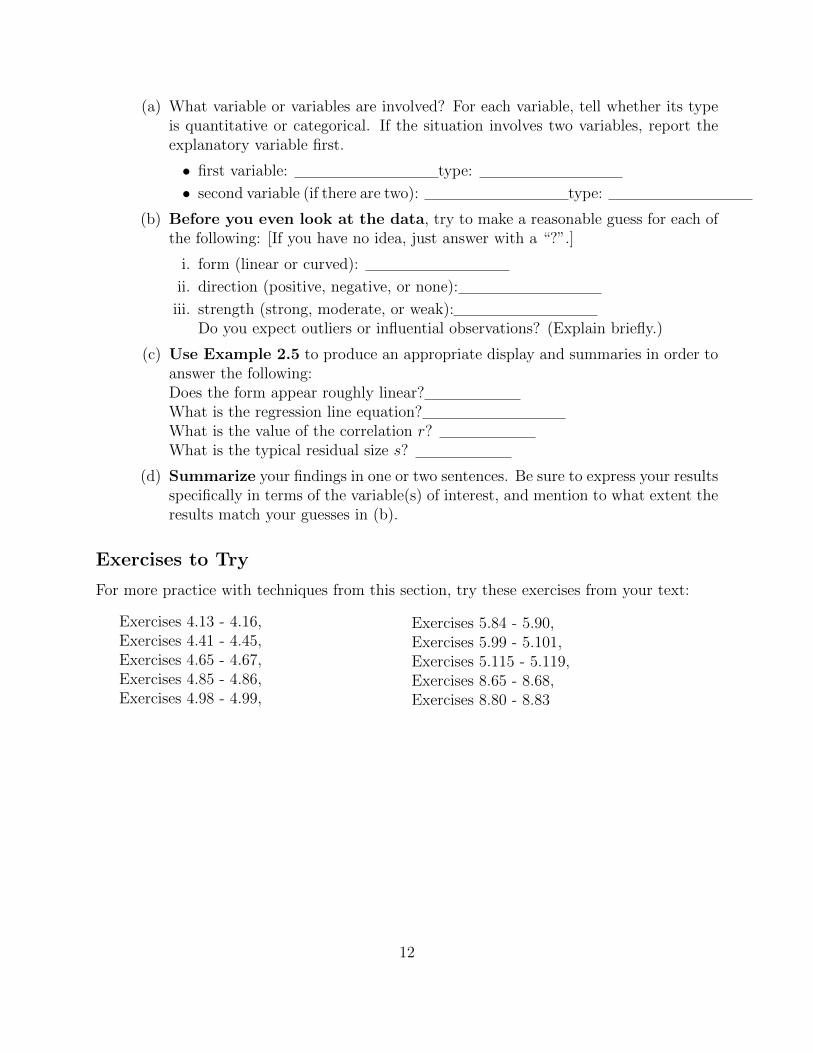
(a) What variable or variables are involved? For each variable, tell whether its typeis quantitative or categorical. If the situation involves two variables, report theexplanatory variable first.
• first variable: type:
• second variable (if there are two): type:
(b) Before you even look at the data, try to make a reasonable guess for each ofthe following: [If you have no idea, just answer with a “?”.]
i. form (linear or curved):
ii. direction (positive, negative, or none):
iii. strength (strong, moderate, or weak):Do you expect outliers or influential observations? (Explain briefly.)
(c) Use Example 2.5 to produce an appropriate display and summaries in order toanswer the following:Does the form appear roughly linear?What is the regression line equation?What is the value of the correlation r?What is the typical residual size s?
(d) Summarize your findings in one or two sentences. Be sure to express your resultsspecifically in terms of the variable(s) of interest, and mention to what extent theresults match your guesses in (b).
Exercises to Try
For more practice with techniques from this section, try these exercises from your text:
Exercises 4.13 - 4.16,Exercises 4.41 - 4.45,Exercises 4.65 - 4.67,Exercises 4.85 - 4.86,Exercises 4.98 - 4.99,
Exercises 5.84 - 5.90,Exercises 5.99 - 5.101,Exercises 5.115 - 5.119,Exercises 8.65 - 8.68,Exercises 8.80 - 8.83
12

PART 3: PROBABILITY
Examples for Part 3: Probability
Example 3.1 We can use SPSS to take a random sample of, say, 10 heights from those ina data column.
1. Choose Data>Select Cases
2. Select Random Sample of cases
3. Click Sample...
4. Select Exactly and type 10 in the first text box
5. Type 466 (total number of observations) in the second text box
6. Click Continue
7. Click OK. Note: SPSS puts a / on non-selected cases. When performing analysis,only the selected cases will be included.
Example 3.2: To undo this and continue to analyze all cases,
1. Click Data>Select Cases
2. Select All cases
3. Click OK.
Lab Activities for Part 3: Probability
3.1 Use Example 3.1 to randomly sample (without replacement) 5 values from the col-umn Cash and report the total amount of cash carried by the five selected students.
3.2 The probability that at least two people in a group of 23 have the same birthday isapproximately 0.50; the probability that at least two people in a group of 60 have thesame birthday is approximately 0.99?
1. Use Example 3.2 to set up a column of numbers from 1 to 365 in SPSS, repre-senting all the possible birthday dates in a year.
2. Sample 23 dates with replacement, sort them, and check if there are duplicates.Take a total of twenty such samples with replacement, and report what proportioncontain duplicates: Is it close to 0.50?
3. Sample 60 dates with replacement, sort them, and check if there are duplicates.Take a total of twenty such samples with replacement, and report what proportioncontain duplicates: Is it close to 0.99?
13
PART 4: STATISTICAL INFERENCE
Examples for Part 4: Statistical Inference
C Single Categorical Variable
Recall: A Z-test is used when testing hypotheses about population proportions.
Example 4.1A: Use SPSS to do inference about the population proportion of males/females;specifically, test if the sample represent a population with more than 40% who are male.Note that the following procedure only works for categorical variables like Sex that havejust 2 possibilities. Since Sex is a String variable, we will first have to convert it to anumeric response. Including a display is a good habit to acquire in using software toperform inference.
Binomial Options Explained
1. Create a Pie Chart as show above
2. Click Transform>Automatic Recode
3. Select Sex and click the right arrow
4. In the New Name text box type RecodedSex
5. Click Add New Name
6. Click OK
7. Click Analyze>Nonparametric Tests>Binomial
8. Specify RecodedSex in the Test Variable List text box
9. Change the Test Proportion to .6 (Since male isn’t the first value in the column,we must enter 1- the proportion we wish to test).
10. Click OK
Example 4.1B: Use MINITAB to test if the population proportion preferring thecolor green could be one-eighth (0.125), starting with a piechart to display the data.These steps may be followed if the variable of interest has more than 2 possibilities.
1. Create a Pie Chart as described above
2. Click Transform>Recode into Different Variables
3. Select Color and press the right arrow
4. In the Name text box, type RecodedColor
5. Click Change
6. Click Old and New Values
7. Under Old Value, in the Value text box, type green
14
8. Under New Value, in the Value text box, type 1
9. Click Add
10. Under Old Value, select All other values
11. Under New Value, in the Value text box, type 2
12. Click Add
13. Click Continue
14. Click OK
15. Click Analyze>Nonparametric tests>Binomial
16. Specify RecodedColor in the Test Variable List text box
17. Since green is not the first color in the column, in the Test Proportion we will use1- the proposed proportion. Enter .875
18. Click OK
Q Single Quantitative Variable
Recall: A Z-test is used to test hypotheses about a single population mean (orconstruct confidence intervals) when σ is known. A t-test is used to test hypothesesabout a population mean (or construct confidence intervals) with σ is unknown.
Example 4.2A: (σ known) SPSS does not provide functionality to complete a testor construct a confidence interval when σ is known.
Example 4.2B: (σ unknown) Now assume Verbal SAT scores of surveyed studentsmembers to be a random sample taken from scores of all students at a particularuniversity, whose mean and standard deviation are unknown. Use sample scores toobtain a 99% confidence interval for the population mean score. Explore OptionsExplained
1. Choose Analyze>Descriptive Statistics>Explore...
2. Specify Verbal in the Dependent List
3. Click Statistics
4. Type 99 in the Confidence Interval for Mean text box
5. Click Continue
6. Click Plots
7. Check Histogram
8. Click Continue
9. Click OK
Now test the null hypothesis that Verbal SAT scores of surveyed students are a randomsample taken from a population with a mean of 600 when σ is unknown.
15

1. Choose Analyze>Compare Means>1-Sample T Test...
2. Specify Verbal in the Test Variables text box.
3. Type 600 in the Test Value text box
4. Click OK.
C→Q Relationship between Categorical Explanatory and Quantitative ResponseVariables
Recall: A paired t-test is used to test hypotheses involving two population meanswhen the two samples involved are dependent. A two-sample t-test is used to testhypotheses involving two population means when the two samples involved are inde-pendent. An ANOVA is used to test hypotheses involving more than two populationmeans.
Example 4.3A: (Paired design) Do students’ dads tend to be older than their moms?Test the null hypothesis that the mean of differences (ages of dads minus ages of moms)for the larger population is zero, against the alternative that the mean of differences ispositive. Paired Options Explained
1. Choose Analyze>Compare Means>Paired Samples T Test...
2. In the Variable1 text box, specify DadAge
3. In the Variable2 text box, specify MomAge
4. Click OK
Example 4.3B: (Two-sample design)
Use SPSS to check if, on average, there is a difference between amount of cash carriedby female and male students. Procedure may or may not be pooled. IndependentSamples T Test Options Explained
1. Choose Analyze>Compare Means>Independent-Samples T Test...
2. Specify Cash in the Test Variables text box.
3. Specify Sex in the Grouping Variable text box.
4. Click Define Groups...
5. In the Group 1 text box, type male
6. In the Group 2 text box, type female
7. Click Continue
8. Click OK. Note: Both the test for equal variances and for unequal variancesare provided.
16

Example 4.3C: (Several-sample design) Use SPSS to see if there is a significantdifference in mean earnings of freshmen, sophomores, juniors, and seniors in the class.Include side-by-side boxplots to display the data. Since this has missing data and alsoan “other” category, we will want to exclude those cases. CAUTION: It is temptingto use the One-Way ANOVA option, but this option does not support categoricalvariables that are nonnumeric.
1. Click Data>Select Cases
2. Select If condition is satisfied
3. Click If...
4. Input the formula Year~=“ ” & Year~=“other”
5. Click Continue
6. Click Analyze>Compare Means>Means
7. Specify Earned in the Dependent List
8. Specify Year in the Independent List
9. Click Options...
10. Check Anova table and eta
11. Click Continue
12. Click OK
C→C Relationship between two Categorical Variables
Recall: A χ2 test is used to determine if there two categorical variables are indepen-dent or dependent.
Example 4.4: Use SPSS to check for a relationship between major being decided ornot, and living situation (on or off campus). Again, there are missing data values thatwe do not want to include, so we will exclude them. Crosstabs Options Explained
1. Click Data>Select Cases
2. Select If condition is satisfied
3. Click If...
4. In the text box, type Dec~=“ ” & Live~=“ ”
5. Click Continue
6. Click OK
7. Choose Analyze>Descriptive Statistics>Crosstabs
8. Consider which should be the explanatory variable; in this case, neither of thevariables is a natural choice for the explanatory variable, because a confoundingvariable is responsible for the relationship. We’ll specify Dec in the Rows textbox and Live in the Column(s) text box.
17
9. Click Statistics...
10. Check Chi-Square
11. Click Continue
12. Click Cell...
13. Click Expected under Counts and Row under Percentages
14. Click Continue
15. Click Display clustered bar charts
16. Click OK
Lab Activities for Part 4: Statistical Inference
4.1 The proportion of American adults who smoked at the time the students were surveyedwas 0.25. Was the proportion significantly lower for university students?
(a) What variable or variables are involved? For each variable, tell whether its typeis quantitative or categorical. If the situation involves two variables, report theexplanatory variable first.
• first variable: type:
• second variable (if there are two): type:
(b) Before you even look at the data, give a rough guess for the populationproportion of students who smoked . Then formulate null and al-ternative hypotheses to test if the population proportion was necessarily less than0.25.H0 :Ha :Do you suspect that there will be enough evidence to reject H0?
(c) Use Example 4.1 to display the data, then find a 95% confidence interval forthe unknown population proportion.Test your hypotheses, making sure to opt for the correct alternative: the P -valueis . Do you reject H0?
(d) State your results: since you did or did not reject H0, what do you concludeabout the unknown population proportion? Be sure to express your results specif-ically in terms of the variable(s) of interest, and mention to what extent the resultsmatch your suspicions in (b).
4.2A (σ known) Math SAT scores are assumed to have a standard deviation of 100. Is themean Math SAT score of all intro Stat students at a particular university 600?
18

(a) What variable or variables are involved? For each variable, tell whether its typeis quantitative or categorical. If the situation involves two variables, report theexplanatory variable first.
• first variable: type:
• second variable (if there are two): type:
(b) Before you even look at the data, formulate null and alternative hypotheses aboutthe population mean µ.H0 :Ha :Do you suspect that there will be enough evidence to reject H0?
(c) Use Example 4.2A to carry out a z test, specifying σ and making sure to optfor the correct alternative (<, 6=, or >); include a display of the data. What isthe P -value?Do you reject H0?Give a 95% confidence interval for µ:[Note: this was automatically provided if your alternative was 6=; otherwise, repeatthe procedure, this time opting for a two-sided alternative.]
(d) State your results: based on the outcome (you did or did not reject H0), whatdo you conclude about the unknown population mean? Be sure to express yourresults specifically in terms of the variable(s) of interest, and mention to whatextent the results match your suspicions in (b).
4.2B (σ unknown) Adults in the U.S. average 7 hours of sleep a night. Is this also the meanfor the population of students at a particular university?
(a) What variable or variables are involved? For each variable, tell whether its typeis quantitative or categorical. If the situation involves two variables, report theexplanatory variable first.
• first variable: type:
• second variable (if there are two): type:
(b) Before you even look at the data, formulate null and alternative hypothesesabout the population mean µ.H0 :Ha :Do you suspect that there will be enough evidence to reject H0?
(c) Note: When σ is unknown, you should carry out a test of your hypotheses using at procedure, not z. Use Example 4.2B to carry out the one-sample t procedure,making sure to opt for the correct alternative (<, 6=, or >); include a display ofthe data. What is the P -value?Do you reject H0?
19

Give a 95% confidence interval for µ: [Note: this was auto-matically provided if your alternative was 6=; otherwise, repeat the t procedure,this time opting for a two-sided alternative.]
(d) State your results: based on the outcome (you did or did not reject H0), whatdo you conclude about the unknown population mean? Be sure to express yourresults specifically in terms of the variable(s) of interest, and mention to whatextent the results match your suspicions in (b).
4.3A Overall, is there a positive mean difference between the number of minutes studentsspend on the computer versus the number of minutes they spend exercising? (Theinitial suspicion is that students spend more time on the computer than they do exer-cising.)
(a) What variable or variables are involved? For each variable, tell whether its typeis quantitative or categorical. If the situation involves two variables, report theexplanatory variable first.
• first variable: type:
• second variable (if there are two): type:
(b) Before you even look at the data, formulate null and alternative hypothesesabout the population mean difference µd.H0 :Ha :Do you suspect that there will be enough evidence to reject H0?
(c) Use Example 4.3A to carry out a paired t procedure, making sure to opt forthe correct alternative (<, 6=, or >); include a display of the data. What is theP -value?Do you reject H0?
(d) State your results: based on the outcome (you did or did not rejectH0), what doyou conclude about the unknown population mean difference? Be sure to expressyour results specifically in terms of the variable(s) of interest, and mention towhat extent the results match your suspicions in (b).
4.3B Is the mean number of credits taken the same for all on- and off-campus students at aparticular university?
(a) What variable or variables are involved? For each variable, tell whether its typeis quantitative or categorical. If the situation involves two variables, report theexplanatory variable first.
• first variable: type:
• second variable (if there are two): type:
20

(b) Before you even look at the data, formulate null and alternative hypothesesabout the difference µ1 − µ2 between population means for the two groups. [Thenull hypothesis usually states that this difference is zero.]H0 :Ha :Do you suspect that there will be enough evidence to reject H0?
(c) Use Example 4.3B to carry out a two-sample t procedure, making sure to optfor the correct alternative (<, 6=, or >); include a display of the data. What isthe P -value?Do you reject H0?
(d) State your results: based on the outcome (you did or did not reject H0), whatdo you conclude about the unknown difference between population means? Besure to express your results specifically in terms of the variable(s) of interest, andmention to what extent the results match your suspicions in (b).
4.3C In general, is mean age the same for students who wear contact lenses, glasses, orneither?
(a) What variable or variables are involved? For each variable, tell whether its typeis quantitative or categorical. If the situation involves two variables, report theexplanatory variable first.
• first variable: type:
• second variable (if there are two): type:
(b) Before you even look at the data, formulate null and alternative hypothesesabout the population means.H0 :Ha :Do you suspect that there will be enough evidence to reject H0?
(c) Use Example 4.3C to carry out an ANOVA procedure; include a display of thedata. What is the P -value?Do you reject H0?
(d) State your results: based on the outcome (you did or did not reject H0), whatdo you conclude about the various population means? Be sure to express yourresults specifically in terms of the variable(s) of interest, and mention to whatextent the results match your suspicions in (b).
4.4 Is there a statistically significant relationship between whether or not a student smokesand whether the student lives on or off campus?
21

(a) What variable or variables are involved? For each variable, tell whether its typeis quantitative or categorical. If the situation involves two variables, report theexplanatory variable first.
• first variable: type:
• second variable (if there are two): type:
(b) Before you even look at the data, formulate null and alternative hypothesesabout the relationship between those variables.H0 :Ha :Do you suspect that there will be enough evidence to reject H0?
(c) Use Example 4.4 to construct a two-way table of counts and row percents,and carry out a chi-square test; include a display of the data. What is the P -value?Do you reject H0?
(d) State your results: based on the outcome (you did or did not reject H0), doyou conclude that those variables are related? Be sure to express your resultsspecifically in terms of the variable(s) of interest, and mention to what extent theresults match your suspicions in (b).
4.5 Is there a relationship between the heights of students’ fathers and mothers?
(a) What variable or variables are involved? For each variable, tell whether its typeis quantitative or categorical. If the situation involves two variables, report theexplanatory variable first.
• first variable: type:
• second variable (if there are two): type:
(b) Before you even look at the data, formulate null and alternative hypothesesabout the slope β1 of the population regression line.H0 :Ha :Do you suspect that there will be enough evidence to reject H0?
(c) Use Example 4.5 to display the data and verify that the form is reasonablylinear. Then carry out a regression procedure to test your hypotheses. What isthe P -value?Do you reject H0?
(d) State your results: based on the outcome (you did or did not reject H0), doyou conclude that the population variables are related? Be sure to express yourresults specifically in terms of the variable(s) of interest, and mention to whatextent the results match your suspicions in (b).
22

Exercises to Try
For more practice with techniques from this section, try these exercises from your text:
Exercises 9.32 - 9.35,Exercises 9.68 - 9.71,Exercises 9.93 - 9.95,Exercises 10.73 -10.85,Exercises 11.50 - 11.51,
Exercises 11.70 - 11.73,Exercises 11.80 - 11.103,Exercises 12.44 - 12.54,Exercises 13.50 - 13.58
23

OPTIONS EXPLAINED
Binomial Options Explained
1. The “Options...” button opens a dialog box where descriptive statistics can be re-quested and options for dealing with missing data can be modified.
Return to Example 4.1Explore Options Explained
1. The “Statistics...” button opens a dialog box where the user can request descriptivestatistics, M-estimators, outliers, and percentiles as well as change the confidence levelfor the confidence interval for the mean.
2. The “Plots...” button opens a dialog box where options for boxplots of the data canbe modified and additional plots can be selected.
3. The “Options” button opens a dialog box where options for dealing with missing datacan be modified.
Return to Example 4.2BPaired Options Explained
1. The “Options...” button opens a dialog box where the confidence level for a confidenceinterval can be modified and options for dealing with missing data can be modified.
Return to Example 4.3AIndependent Samples T Test Options Explained
1. The “Options...” button opens a dialog box where the confidence level for a confidenceinterval can be modified and options for dealing with missing data can be modified.
Return to example 4.3BCrosstabs Options Explained
1. The “Format...” button opens a dialog box where you can choose an order for the rowlevel.
Return to Example 4.4
24