SPS 3D Binned Attributes

Nyquist Technology Pty. Ltd.

3D CMP and Binning Computation

3D Binned Attribute displays show the data in 3D SPS Files after

CMP’s have been computed and the resultant CMP locations

binned onto a regular grid of Inlines and Xlines (Crosslines).

The following display types can be produced:

▪ Map Plots of Bin Attributes

▪ Graph Plots of Bin Attributes

▪ Rose Plots

▪ Spider Plots

▪ Necklace Plots

Each of these is discussed in the following slides.

3D CMP’s are calculated from the Shot and Recv coordinates and

the Xdef information read from the SPS files. If necessary, any

errors in the SPS data should be corrected before this is done.

The data is then binned with user specified parameters as shown

top right.

A Bin Calculator utility program can be used to do conversion

between X/Y coordinates and Inline/Xline numbers at discrete

locations as shown bottom right.

Multiple surveys can also be binned onto the one grid. Binned

Attributes can then be computed and all of the above display

types produced. This is discussed last in this presentation.

Bin Calculator – used to compute X/Y coordinates from Inline/Xline

numbers or vice versa for a given set of Bin parameters.

Bin parameters input - The calculated CMP’s are binned with user

specified binning parameters. Bins can be specified in either of two

ways:

▪ Origin, Azimuth and Interval parameters; or

▪ Inputting of three corner points.

.

Bin Attribute Computation and Import

A number of Bin Attributes can be computed on the binned data. These

include the following:

▪ Fold

▪ Minimum Offset

▪ Maximum Offset

▪ Average Offset

▪ Average Trace Interval

Each computation can be limited by Inline, Xline, Offset and Azimuth as

shown above right. This makes it possible to compute Azimuth-Dependent

attributes to enable analysis of the offset and azimuth distributions prior to

any azimuth- or offset-dependent processing.

Bin Attributes can also be imported from external files. The file can contain

either X/Y coordinates or Inline/Xline numbers as the means of location for

the attribute in the file.

A simple text histogram plot can be displayed on any Bin Attribute. This

allows the data ranges to be checked and set prior to plots being produced.

Each Bin Attribute can be displayed either as a Map Plot or as a Graph Plot.

Graph plots can be made in both the Inline and Xline directions.

As the computation time to produce the a Binned Attribute is significant,

particularly for large surveys, the program pre-computes the necessary data

so that the actual display can be done and modified quickly and easily. Up to

twelve different Binned Attributes can be created.

Bin Attribute computation window.

Bin Attribute import window.

Text histogram of a Bin Attribute.

Bin Attribute Maps

Bin Attribute Maps can be plotted with the following features

▪ Colour coding of the attribute.

▪ Grid lines and annotation of Inline and/or Xline line numbers

▪ Geo-referenced background image files.

▪ Over-plot files containing locations of wells, boundaries, roads,

cultural features, etc.

The Shot and/or Recv locations can also be under- or over-plotted

on the display.

Automatic highlighting of line and cursor tracking from other line-

orientated plots can optionally be turned on.

The display can be used as a digitized using the inbuilt digitizer

function.

Example Fold attribute map plot.

Bin Attribute Map Example

Map showing the elevation at the Shot and Recv locations from the SPS Files. Map showing the binned elevation derived from the Shot and Recv elevations.

Azimuth-Dependent Example – Fold Maps

0-60 Deg

300-360 Deg 240-300 Deg 180-240 Deg

120-180 Deg60-120 Deg

Azimuth Dependent Example – Average Offset Maps

0-60 Deg

300-360 Deg 240-300 Deg 180-240 Deg

120-180 Deg60-120 Deg

Attribute Graph Plot Examples

Graph of the Fold along the Inline highlighted in the Map plot. Graph of the Fold along the Xline highlighted in the Map plot.

Rose Plots

Rose Plots show the Offset/Azimuth distribution for an

entire 3D survey. They can be produced with a variety of

offset and azimuth binning options. As seen in the

following examples, they are a good way of getting an

overall picture of the effect of the survey geometry on

these distributions in one plot.

An alternative way at looking at the Survey wide Offset and

Azimuth distributions is to plot these as individual

histogram plots. These are produced using the same

binned Offset and Azimuth datasets as used for a Rose

Plot.

As the computation time to produce the binned offset and

azimuth data necessary to do a Rose plot is significant,

particularly for the large surveys, the program pre-

computes the necessary data so that the actual display

can be done and modified quickly and easily. Up to six

different Rose datasets can be created.

In order to produce Rose datasets the survey must have

had its CMP’s computed but does not have to be binned.

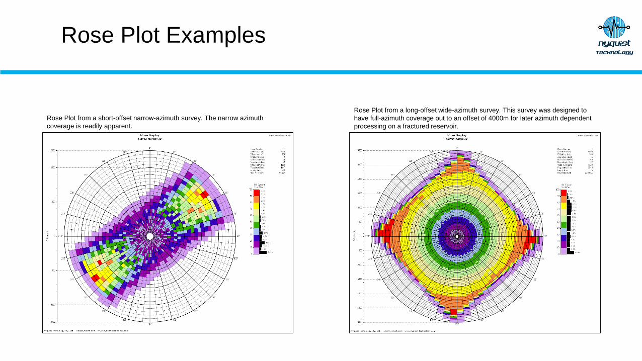
Rose Plot Examples

Rose Plot from a short-offset narrow-azimuth survey. The narrow azimuth

coverage is readily apparent.

Rose Plot from a long-offset wide-azimuth survey. This survey was designed to

have full-azimuth coverage out to an offset of 4000m for later azimuth dependent

processing on a fractured reservoir.

Offset and Azimuth Distribution Plot Examples

Offset (top) and Azimuth (bottom) distributions for a short-offset narrow-azimuth survey. Offset (top) and Azimuth (bottom) distributions for a long-offset wide-azimuth survey.

Necklace Plots

Necklace Plots are produced on Binned data and show

how the Offsets and Azimuths are distributed in individual

Bins. Such plots are useful to see the suitability of a survey

for pre-stack offset and azimuth dependent processing.

Necklace plots can be produced in both the Inline and

Xline domains. Displays in either domain can be made of

either the Offset or Azimuth distribution within each Bin. A

Crossplot of Offset/Azimuth can also be produced. All

displays can use Offset, Azimuth, or Line Number to colour

code the individual plot points.

The Necklace location currently being displayed can be

automatically highlighted on any displayed map plot as

shown at right.

As the computation time to produce the Necklace data is

significant, particularly for large surveys, the program pre-

computes the necessary data so that the actual display

can be done and modified quickly and easily. Up to six

different Necklace datasets can be created.

Necklace Plot – Inline vs Offset Wide-Azimuth Example

Inline vs Offset Necklace Plot for the wide-azimuth long-offset example. Azimuth is used for the colour attribute.

Necklace Plot – Inline vs Azimuth Wide-Azimuth Example

Inline vs Azimuth Plot for the wide-azimuth long-offset example. Offset is used for the colour attribute.

Necklace Plot - Offset vs Azimuth CrossplotWide-Azimuth Example

Inline Offset vs Azimuth Crossplot for the wide-azimuth long-offset

example. Xline number is used for the colour attribute.Xline Offset vs Azimuth Crossplot for the wide-azimuth long-offset

example. Inline number is used for the colour attribute.

Necklace PlotsNarrow-Azimuth Example

Inline vs Offset Necklace Plot

Inline vs Azimuth Necklace Plot

Xline vs Offset Necklace Plot Inline Offset vs Azimuth Crossplot

Xline vs Azimuth Necklace Plot Xline Offset vs Azimuth Crossplot

Binned Necklace PlotsNarrow-Azimuth Example

Inline vs Binned Offset Necklace Plot

Inline vs Binned Azimuth Necklace Plot

Xline vs Binned Offset Necklace Plot Necklace plots can optionally be

binned when displayed.

Binning can be done in either the

Offset or Azimuth domain

depending on the display being

made.

The Vertical Fold can be used as

the colour attribute for binned

displays.

These displays can be used to help

optimise binning parameters prior to

offset or azimuth dependent pre-

processing of the seismic data.

Xline vs Binned Azimuth Necklace Plot

Note: All displays use the Vertical Fold as the colour attribute.

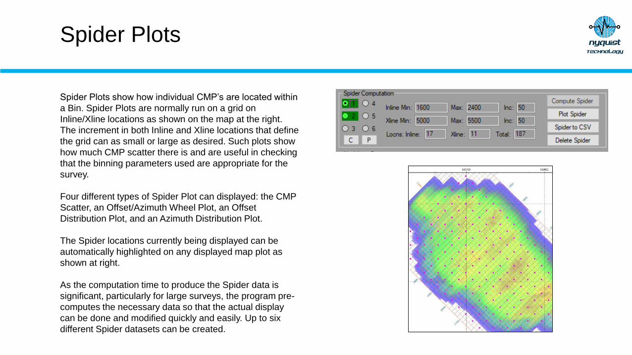
Spider Plots

Spider Plots show how individual CMP’s are located within

a Bin. Spider Plots are normally run on a grid on

Inline/Xline locations as shown on the map at the right.

The increment in both Inline and Xline locations that define

the grid can as small or large as desired. Such plots show

how much CMP scatter there is and are useful in checking

that the binning parameters used are appropriate for the

survey.

Four different types of Spider Plot can displayed: the CMP

Scatter, an Offset/Azimuth Wheel Plot, an Offset

Distribution Plot, and an Azimuth Distribution Plot.

The Spider locations currently being displayed can be

automatically highlighted on any displayed map plot as

shown at right.

As the computation time to produce the Spider data is

significant, particularly for large surveys, the program pre-

computes the necessary data so that the actual display

can be done and modified quickly and easily. Up to six

different Spider datasets can be created.

Spider CMP Scatter Plot Example

Spider CMP Scatter Plot. For this data, the plot indicates that the Binning parameters are probably not

optimal and a small adjustment to the Bin Origin X and Y coordinates is needed.

Spider Offset/Azimuth Wheel Plot Example

Offset/Azimuth Wheel Plot with Offset used as the colour attribute. The plot shows that longer offsets are

only present in the data over a limited azimuth range.

Spider Offset Distribution Plot Example

Offset Distribution Plot with Offset used as the colour attribute. The plot shows the data generally has

reasonably good offset distribution meaning that pre-stack offset-dependent processing should be okay.

Spider Azimuth Distribution Plot Example

Azimuth Distribution Plot with Azimuth used as the colour attribute. The plot shows the data generally has

poor azimuth distribution. This is also clearly evident on the Colour Bar histogram plot.

Multiple Survey Database (MFile)

Multiple individual survey databases (PFiles) can be

combined into one database (MFile) and the resultant

data displayed and binned as if it were the one survey.

For each survey, the SPS data should be read into a

PFile and analysed for any errors as detailed the SPS

Quality Assurance presentation. Any errors in any of the

PFiles should be corrected before being added to an

MFile.

Both 3D and 2D surveys can be added to an MFile.

Up to 100 PFiles can be added to an Mfile.

Map display of an MFile with one 2D and three 3D surveys colour coded by survey.

3D Binning of MFile data - BinSet Manager

The BinSet Manager is used to 3D bin the data in an MFile. A BinSet is

defined by two main inputs:

▪ The PFiles to include in the BinSet.

▪ The bin parameters to use for the binning.

(Note that not all the PFiles in an MFile need to be included in a BinSet.)

Up to 20 different BinSets can be defined in an MFile. This allows different

binning strategies to be tried and compared.

Although primarily for the binning of overlapping 3D surveys, 2D surveys

can also be included in a BinSet if desired.

Only PFiles that have their CMP’s computed can be included in a BinSet.

BinSet Manager Window.

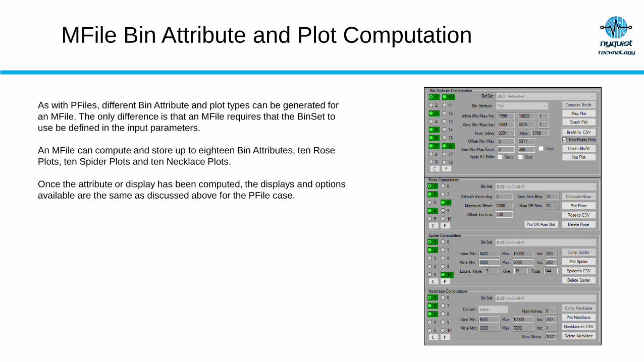
MFile Bin Attribute and Plot Computation

As with PFiles, different Bin Attribute and plot types can be generated for

an MFile. The only difference is that an MFile requires that the BinSet to

use be defined in the input parameters.

An MFile can compute and store up to eighteen Bin Attributes, ten Rose

Plots, ten Spider Plots and ten Necklace Plots.

Once the attribute or display has been computed, the displays and options

available are the same as discussed above for the PFile case.

MFile Bin Attribute Map and Graph Plot Example

MFile Minimum Offset Map Plot. Inline 9272 and Xline 6878 are highlighted.

MFile Minimum Offset Graph Plot Inline 9272

MFile Minimum Offset Graph Plot Xline 6878

MFile Rose Plot Example

MFile Rose Plot with all four example PFiles used.

MFile Offset Distribution with all four example PFiles used.

MFile Azimuth Distribution with all four example PFiles used.

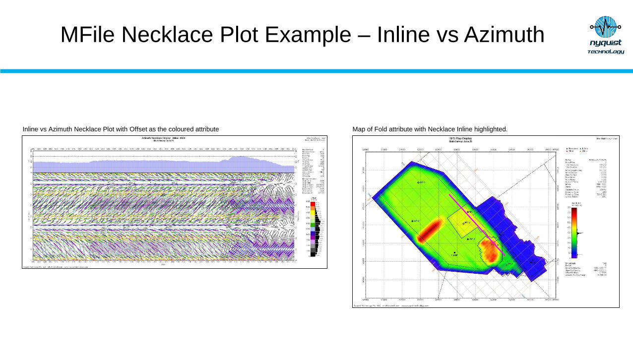
MFile Necklace Plot Example – Inline vs Azimuth

Inline vs Azimuth Necklace Plot with Offset as the coloured attribute Map of Fold attribute with Necklace Inline highlighted.

MFile Spider Plot Example - CMP Scatter Plot

CMP Scatter Spider Plot with Survey as the coloured attribute Map of Fold attribute with Spider locations highlighted.

MFile Production Plot Example

Production Plot of Shot data with surveys colour coded.