Exploratory Analysis of Crash Data

Spring 2013

Sampling FrameSampling frame: the sampling frame is the list of the population (this is a general term) from which the sample is drawn. It is important to understand how the sampling frame defines the population represented.

Example: If the study seeks to identify the safety effects of traffic signals, the sample frame should include a sample of signalized intersections in a given geographical area. If a control group is included, the sampling frame will include sites categorized under this group.

Signalized

Unsignalized

Sig Int #1

Sig Int #2

Unsig Int #1

Unsig Int #2

Sig Int #9

Unsig Int #7

Sampling Frame

Map crashes for Year 1

Map crashes for Year 2

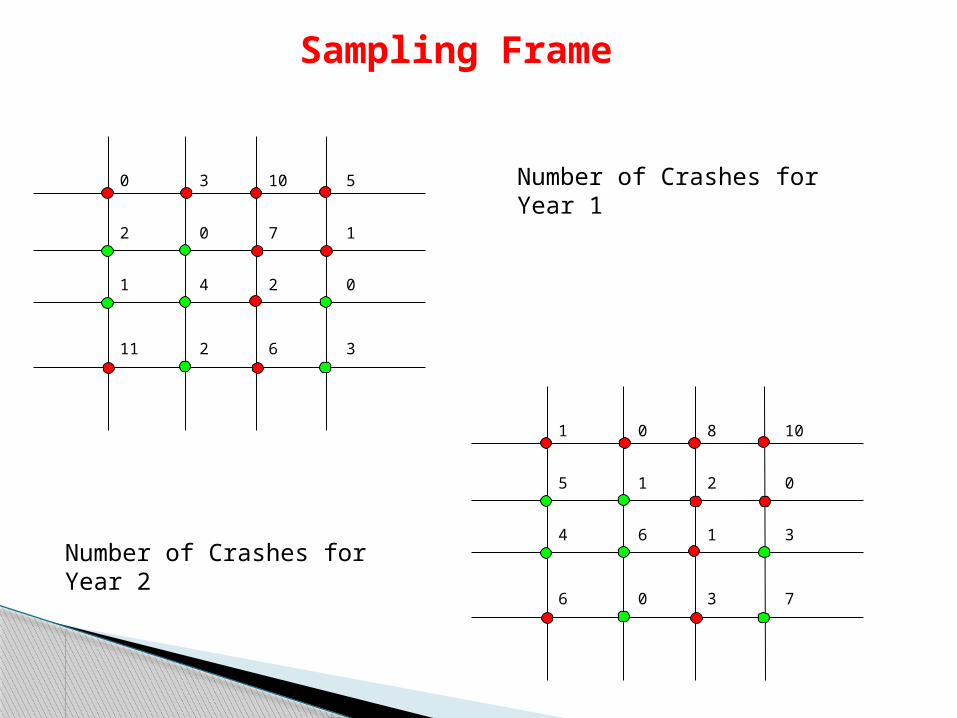
Sampling Frame

0 3 10 5

2 0 7 1

1 4 2 0

11 2 6 3

Number of Crashes for Year 1

Number of Crashes for Year 2

1 0 8 10

5 1 2 0

4 6 1 3

6 0 3 7

Sampling Frame

Intersection Number

Crashes/Year Traffic Flow – Major

Other Site Characteristics*

Year

1 0 11,500 1

2 3 12,000 1

3 10 10,000 1

… … … … 1

9 6 6,300 1

1 1 12,000 2

2 0 12,200 2

… … … … 2

9 3 6,100 2

Signalized Intersections Database

* ex: Nb of lanes, actuated signals, exclusive left-turn lane, etc.

Sampling FrameSignalized Intersections Database

0 1 Crash Count

Year1 2Intersection 1

6 3 Crash Count

Year1 2Intersection 9

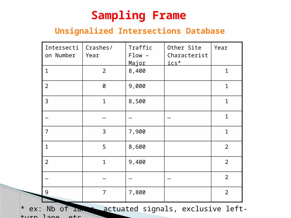
Sampling Frame

Intersection Number

Crashes/Year Traffic Flow – Major

Other Site Characteristics*

Year

1 2 8,400 1

2 0 9,000 1

3 1 8,500 1

… … … … 1

7 3 7,900 1

1 5 8,600 2

2 1 9,400 2

… … … … 2

9 7 7,800 2

Unsignalized Intersections Database

* ex: Nb of lanes, actuated signals, exclusive left-turn lane, etc.

Histograms

0

10

20

30

40

50

60

Injury PDO Injury PDO Injury PDO Injury PDO

Outer Lanes Inner Lanes Inner Lanes Outer Lanes

Southbound Northbound

Location and Serverity of Collision

<=88.1 >90.6 <=90.6 >95.9

10.45%

2.79%

5.23%

1.39%0.70%

5.57%5.92%

18.47%

1.39%

3.83% 3.83%

11.15%

1.05%

5.23% 5.23%

17.77%

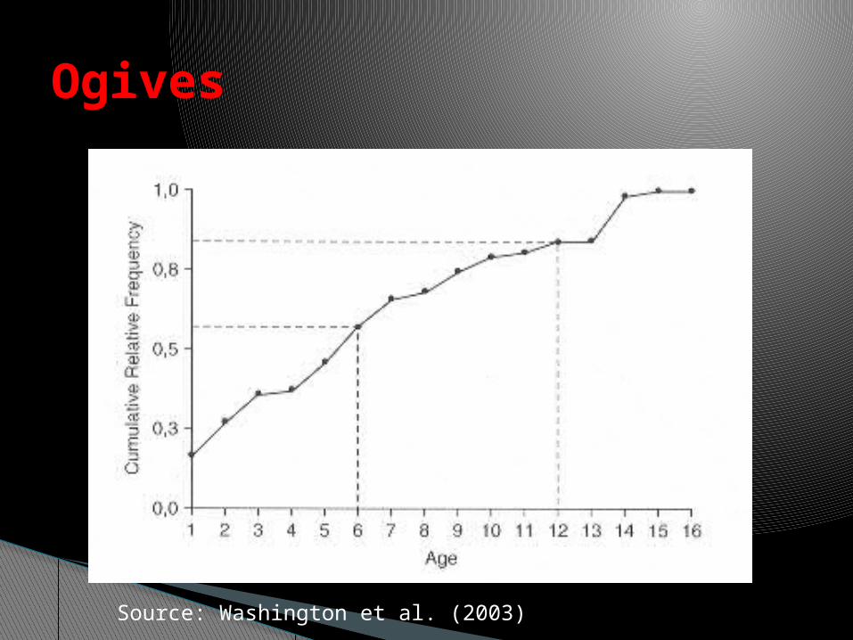
Ogives

Source: Washington et al. (2003)

Box Plots

6.02 6.06 5.97

4.34

7.97

5.9 5.87 6

4.43

7.5

1

2

3

4

5

6

7

8

9

10

Compare Base with Alternative 1 Comfort Level Compare Base with Alternative 2 Comfort Level

Questions

Scatter Diagrams

0

5

10

15

20

25

30

35

40

45

50

0 10000 20000 30000 40000 50000 60000 70000 80000

Traffic Flow

Cra

shes

per

Yea

r

Scatter Diagrams

Bar and Line Charts

Source: Washington et al. (2003)

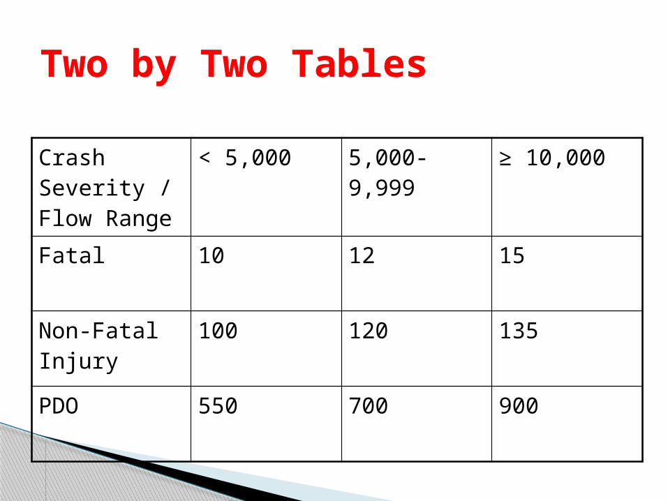
Two by Two Tables

Crash Severity / Flow Range

< 5,000 5,000-9,999 ≥ 10,000

Fatal 10 12 15

Non-Fatal Injury

100 120 135

PDO 550 700 900

High-Rate

Mid-Rate

Low-Rate

Maps

Maps – GIS Information

http://www.saferoadmaps.org/home/

Confidence Intervals

Statistics are usually calculated from samples, such as the sample average X, variance s2, the standard deviation s, are used to estimate the population parameters. For instance:

X is used as an estimate of the population μx

s2 is used as an estimate of the population variance σ2

Interval estimates, defined as Confidence Intervals, allow inferences to be drawn about the population by providing an interval, a lower and upper value, within which the unknown parameter will lie with a prescribed level of confidence. In other words, the true value of the population is assumed to be located within the estimated interval.

Confidence Intervals

Confidence Interval for μ and known σ2

95% CI

90% CI

Any CI

0.95 1.96 1.96P X Xn n

1.96Xn

1.645Xn

/ 2X Zn

Confidence Intervals

Compute the 95% confidence interval for the mean vehicular speed. Assume the data is normally distributed. The sample size is 1,296 and the sample mean X is 58.86. Suppose the population standard deviation (σ) has previously been computed to be 5.5.

Confidence Intervals

Compute the 95% confidence interval for the mean vehicular speed. Assume the data is normally distributed. The sample size is 1,296 and the sample mean X is 58.86. Suppose the population standard deviation (σ) has previously been computed to be 5.5.

Answer

1.96Xn

5.558.86 1.96 58.86 0.30

1,296

58.56,59.16CI

Confidence Intervals

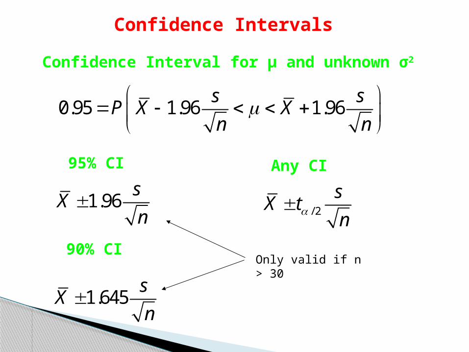
Confidence Interval for μ and unknown σ2

95% CI

90% CI

Any CI

Only valid if n > 30

0.95 1.96 1.96s s

P X Xn n

1.96s

Xn

1.645s

Xn

/ 2

sX t

n

Confidence Intervals

Same example: Compute the 95% confidence interval for the mean vehicular speed. Assume the data is normally distributed. The sample size is 1,296 and the sample mean X is 58.86. Now, suppose a sample standard deviation (s) has previously been computed to be 4.41.

Answer

1.96s

Xn

4.4158.86 1.96 58.86 0.24

1,296

58.62,59.10CI

Confidence Intervals

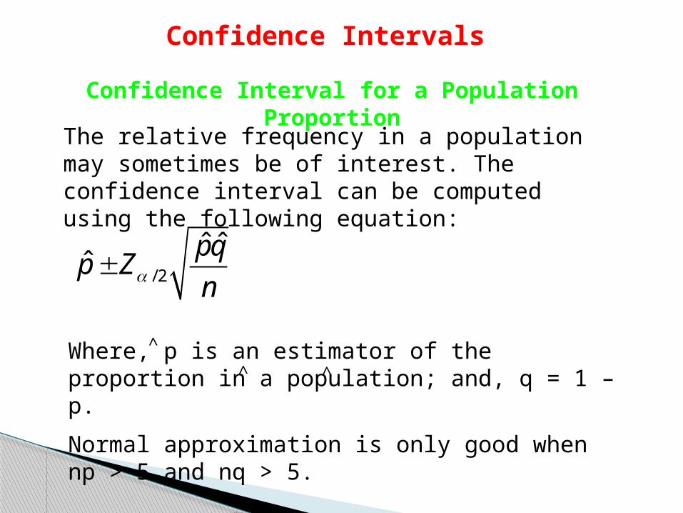
Confidence Interval for a Population Proportion

The relative frequency in a population may sometimes be of interest. The confidence interval can be computed using the following equation:

Where, p is an estimator of the proportion in a population; and, q = 1 – p.

Normal approximation is only good when np > 5 and nq > 5.

^

^ ^

/ 2

ˆ ˆˆ

pqp Z

n

Confidence Intervals

A transportation agency located in a small city is interested to know the percentage of people who were involved in a collision during the last calendar year. A random sample is conducted using 1000 drivers. From the sample, it was found that 110 drivers were involved in at least one collision. Compute the 90% CI.

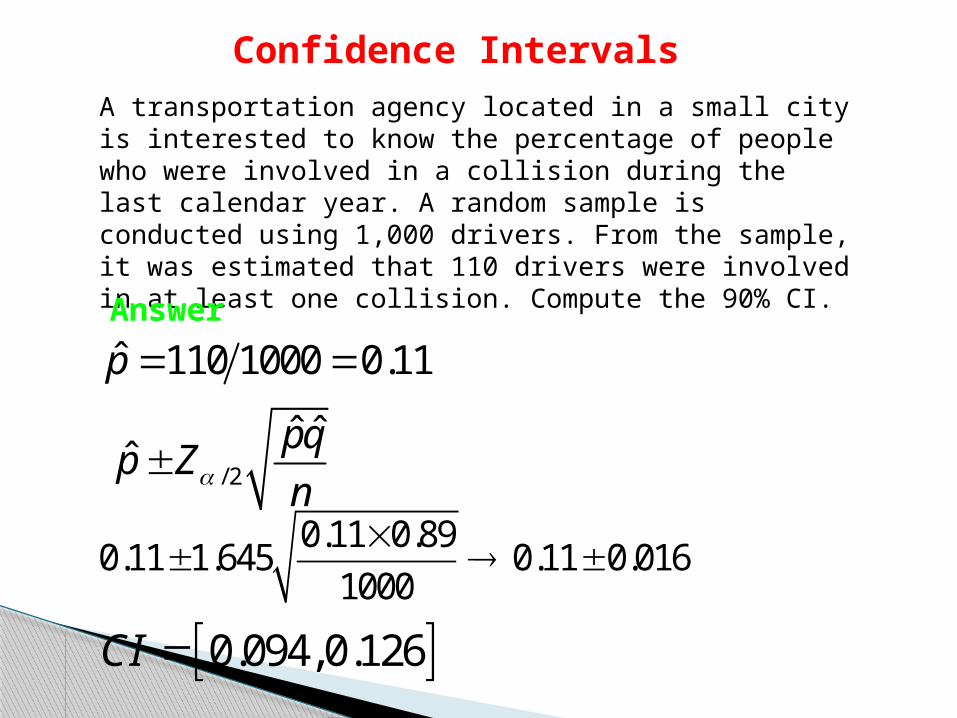
Confidence IntervalsA transportation agency located in a small city is interested to know the percentage of people who were involved in a collision during the last calendar year. A random sample is conducted using 1,000 drivers. From the sample, it was estimated that 110 drivers were involved in at least one collision. Compute the 90% CI.

Answer

/ 2

ˆ ˆˆ

pqp Z

n

ˆ 110 1000 0.11p ˆ 1 0.11 0.89q

0.11 0.890.11 1.645 0.11 0.016

1000

0.094,0.126CI

Population Proportion

6.02 6.06 5.97

4.34

7.97

5.9 5.87 6

4.43

7.5

1

2

3

4

5

6

7

8

9

10

Compare Base with Alternative 1 Comfort Level Compare Base with Alternative 2 Comfort Level

Questions

Confidence Intervals

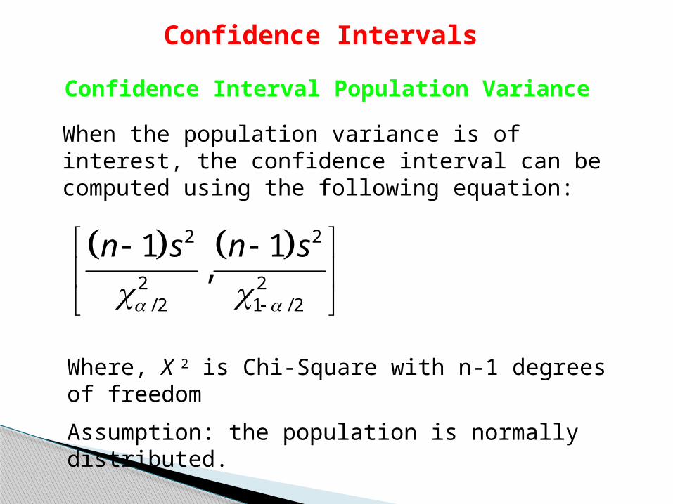
Confidence Interval Population Variance

When the population variance is of interest, the confidence interval can be computed using the following equation:

Where, X 2 is Chi-Square with n-1 degrees of freedom

Assumption: the population is normally distributed.

2 2

2 2/ 2 1 / 2

1 1,

n s n s

Confidence Intervals

Taking the same example before on the vehicular speed, compute the confidence interval (95%) for variance for the speed distribution. A sample of 100 vehicles has shown a variance equal to 19.51 mph.

Confidence Intervals

Taking the same example before on the vehicular speed, compute the confidence interval (95%) for variance for the speed distribution. A sample of 100 vehicles has shown a variance equal to 19.51 mph.

Answer Taken from Chi-Square Table 2 2

2 2/ 2 1 / 2

1 1,

n s n s

99 19.51 99 19.51

,129.56 74.22

15.05,26.02

The Chi-Square Goodness-of -fit

Non-parametric test useful for observations that are assumed to be normally distributed. Need to have more than 5 observations per cell. The test statistic is

If the value on the right-hand side is less than the Chi-Square with n-1 degrees of freedom, the observed and estimated values are the same. If not, the observed and estimated values are not the same.

You can also perform this test for two-way contingency tables.

2

2/ 2

1

ni i

i i

O P

P