Spread spectrum techniques for seismic data acquisition · 2020-01-17 · Spread spectrum...
20
Spread spectrum techniques CREWES Research Report — Volume 24 (2012) 1 Spread spectrum techniques for seismic data acquisition Joe Wong ABSTRACT Mechanical and piezoelectric vibrators are controllable seismic sources used in seismic surveys for data acquisition. In standard industry practice, these sources usually are controlled by frequency-sweep pilot signals. However, spread spectrum techniques, widely used in many fields of science and engineering for obtaining accurate estimates of impulse responses of linear systems, have received attention as pilots for vibrating sources. Spread spectrum techniques are most commonly based on special periodic functions known as pseudorandom binary sequences (PRBSs). In this report, we will examine the properties of two types of PRBS, maximal-length sequences and Gold codes, and see how they can be applied to seismic data acquisition. We will compare the relative merits of using the two alternatives, m-sequences and Gold codes, as pilots for driving vibrating seismic sources. INTRODUCTION Spread spectrum techniques have a long history of application in many fields of science and engineering. Notable examples are their crucial use in wireless communications and in satellite global navigation and positioning systems (GNSS, GPS). The most common spread spectrum techniques are based on the properties of pseudorandom binary sequences (PRBSs) such as maximal length sequences (m-sequence) and the closely related Gold codes. The special characteristics of m-sequences have prompted numerous researchers to use them for analyzing linear systems (Engelberger and Benjamin, 2005). They have been incorporated into long-range radar and sonar applications where signal-to-noise enhancement is crucial. For example, the earliest experiments in detecting radar echoes from Venus employed m-sequences (Price et al., 1959). Behringer et al. (1982) and Dushaw et al. (1999) studied fluctuations in seawater acoustic velocities across thousands of kilometers using PRBS-coded sonar signals. Sachs et al. (2003) have described how modern short-range radar systems have adopted m-sequence coding. Duncan et al. (1980) employed m-sequence signals in a controlled source audiofrequency magnetotelluric (CSAMT) experiment. Ziolkowski et al. (2011) applied m-sequence PRBSs in CSEM surveys over an offshore gas deposit. High-resolution seismic imaging of oil and gas reservoirs may require wavelengths on the order of several meters to several tens of meters. In typical reservoir rocks, the frequencies must be in the range 200 to 2000 Hz (Harris et al., 1995; Fogues et al., 2006). Such frequencies can be produced easily by using piezoelectric materials as transducers. However, the output mechanical power of piezoelectric sources is low, and techniques for signal-to-noise enhancement must be employed to obtain good seismograms across useful distances. To this end, Harris et al. (1995) and Fogues et al. (2006) used cross-correlation and frequency sweeps with their piezoelectric sources. Alternatively, Wong et al. (1983,
Transcript of Spread spectrum techniques for seismic data acquisition · 2020-01-17 · Spread spectrum...

Spread spectrum techniques
CREWES Research Report — Volume 24 (2012) 1
Spread spectrum techniques for seismic data acquisition
Joe Wong
ABSTRACT Mechanical and piezoelectric vibrators are controllable seismic sources used in
seismic surveys for data acquisition. In standard industry practice, these sources usually are controlled by frequency-sweep pilot signals. However, spread spectrum techniques, widely used in many fields of science and engineering for obtaining accurate estimates of impulse responses of linear systems, have received attention as pilots for vibrating sources. Spread spectrum techniques are most commonly based on special periodic functions known as pseudorandom binary sequences (PRBSs). In this report, we will examine the properties of two types of PRBS, maximal-length sequences and Gold codes, and see how they can be applied to seismic data acquisition. We will compare the relative merits of using the two alternatives, m-sequences and Gold codes, as pilots for driving vibrating seismic sources.
INTRODUCTION Spread spectrum techniques have a long history of application in many fields of science and engineering. Notable examples are their crucial use in wireless communications and in satellite global navigation and positioning systems (GNSS, GPS). The most common spread spectrum techniques are based on the properties of pseudorandom binary sequences (PRBSs) such as maximal length sequences (m-sequence) and the closely related Gold codes.
The special characteristics of m-sequences have prompted numerous researchers to use them for analyzing linear systems (Engelberger and Benjamin, 2005). They have been incorporated into long-range radar and sonar applications where signal-to-noise enhancement is crucial. For example, the earliest experiments in detecting radar echoes from Venus employed m-sequences (Price et al., 1959). Behringer et al. (1982) and Dushaw et al. (1999) studied fluctuations in seawater acoustic velocities across thousands of kilometers using PRBS-coded sonar signals. Sachs et al. (2003) have described how modern short-range radar systems have adopted m-sequence coding. Duncan et al. (1980) employed m-sequence signals in a controlled source audiofrequency magnetotelluric (CSAMT) experiment. Ziolkowski et al. (2011) applied m-sequence PRBSs in CSEM surveys over an offshore gas deposit.
High-resolution seismic imaging of oil and gas reservoirs may require wavelengths on the order of several meters to several tens of meters. In typical reservoir rocks, the frequencies must be in the range 200 to 2000 Hz (Harris et al., 1995; Fogues et al., 2006). Such frequencies can be produced easily by using piezoelectric materials as transducers. However, the output mechanical power of piezoelectric sources is low, and techniques for signal-to-noise enhancement must be employed to obtain good seismograms across useful distances. To this end, Harris et al. (1995) and Fogues et al. (2006) used cross-correlation and frequency sweeps with their piezoelectric sources. Alternatively, Wong et al. (1983,

Wong
2 CREWES Research Report — Volume 24 (2012)
1987), Hurley (1983), Yamamoto et al. (1994), and Wong (2000) chose cross-correlation with m-sequences for their piezoelectric vibrators.
Seismic surveys can be broadly considered as attempts to determine the elastic-wave impulse response of a geological environment. In this context, spread spectrum techniques based on m-sequences and Gold codes can be profitably exploited for seismic data acquisition when the source is a controlled vibrator. Pecholcs et al. (2010) and Sallas et al (2011; 2008) have described using modified Gold sequences as pilot signals to drive multiple vibrators simultaneously for land reflection surveys.
This report examines the properties of m-sequences and Gold codes, and evaluates their advantages and disadvantages when they are used as pilot signals to control vibrating seismic sources. Algorithms for generating m-sequences and Gold sequences and information on their most important properties are presented in the Appendices.
m-SEQUENCES AND GOLD CODES Maximal-length sequences (or m-sequences) are well-defined mathematical constructs intimately connected with so-called primitive or irreducible polynomials (Watson, 1962). In practice, m-sequences are easily produced by logic statements in software. They also can be generated electronically by simple circuits known as linear shift registers (Holmes, 2007; Golomb and Gong, 2005). A particular m-sequence is a periodic stream of 1’s and -1’s characterized by its degree 𝑚, its fundamental length L, and its base period 𝑡𝑏. The sequence fundamental length L is given by
𝐿 = 2𝑚 − 1 , (1)
where m is a positive integer. The base period is the shortest time in the sequence between transitions from one binary value to the other. The sequence is periodic, and repeats itself after a time
𝑇𝑚 = 𝐿 ∙ 𝑡𝑏 . (2)
For seismic applications, it is convenient to express 𝑇𝑚 in milliseconds. For digitized versions, we also specify the sample time 𝑡𝑠, with
𝑡𝑠 = 𝑡𝑏/𝑟 , (2)
where 𝑟 is an integer, typically equal to 1, 2, 4, or 16, that determines oversampling of the sequence. The over-sampled length is equal to 𝑟𝐿 points.
The autocorrelation of a sampled m-sequence is also periodic, showing a series of triangular peaks with peak value equal to 𝑟𝐿 and off-peak values equal to −𝑟. If we remove the factor 𝑟, we obtain scaled peak and off-peak values of 𝐿 and -1, respectively. These autocorrelation values are fundamental properties of any m-sequence. The widths of the triangles extend from −𝑟𝐿 samples to +𝑟𝐿 samples symmetrically about the peaks.
A set of Gold codes is constructed from an optimal or preferred pair of m-sequences using the theory presented by Gold (1967). The set is characterized by the degree and base period 𝑡𝑏 of the optimal pair of generating m-sequences. How the preferred pair is combined to produce individual Gold codes is explained in Appendix B. Each member

Spread spectrum techniques
CREWES Research Report — Volume 24 (2012) 3
of the set is also periodic with binary values of -1 and 1. All members of the set have autocorrelations that approximate the delta function. However, their cross-correlations are weakly coupled, i.e., they are not zero. The maximum and minimum values of the cross-correlations oscillate with lag time between predictable small values less than the autocorrelation peak values. From this perspective, the set of related Gold codes can be considered to be quasi-orthogonal. This property can be exploited for simultaneous multiple-vibrator operation in land seismic acquisition (Pecholcs et al., 2010; Sallas et al., 2011; Wong, 2012).
A defining characteristic of a perfectly random signal or pure noise is that its autocorrelation is a delta function. The autocorrelation peaks of an m-sequence or a Gold code approximate the delta function, and the approximation become increasingly better as the degree m and the length L increase. For this reason, both these periodic sequences are referred to as pseudorandom binary sequences, or PRBS.
Auto- and cross-correlations are fundamental to the useful properties of m-sequences and Gold codes. Because they are periodic, correlation between two sequences can be done in a circular fashion, i.e., using one period of each with wrap-around. When calculating the lagged sums using single cycles, if the first sequence runs off the end of the second sequence, its off-end values wraps around to the beginning of the second sequence to complete the correlation. In this report, all correlations and convolutions involving m-sequences and Gold codes will be done in circular fashion.
FIG. 1: Left: Acquisition with a liner frequency sweep from 10Hz to 200Hz, sweep time = 10s, and listen time = 1s. Right: Acquisition with an m-sequence PRBS with m = 7, L = 127, tb = 1.0ms, ts = 1ms. (a) Plots of the sweep and PRBS pilot signals driving a vibrator source; (b) delayed sweep and shifted PRBS signals with wrap-around; (c) cross-correlation of original pilots in (a) with delayed/shifted pilots in b; (d) a source wavelet; (e) convolutions of the source wavelet with the delayed/shifted pilots b; (f) cross-correlation of convolutions in e with the original pilots in a, recovering the wavelet arriving at the times of the correlation peaks in c.

Wong
4 CREWES Research Report — Volume 24 (2012)
SEISMIC ACQUISITION USING SPREAD SPECTUM TECHNIQUES Comparing frequency-sweep and PRBS pilots for vibrator-based acquisition
Figure 1 summarizes the steps that occur when frequency sweeps and pseudorandom sequences are used with vibrating sources for seismic data acquisition. On the left side, we see the steps involved in standard industry practice of using a linear frequency sweep as the pilot signal controlling a vibrator source. On the right side, we see the exact same steps, only in this case a maximal-length sequence PRBS is the pilot. We deliberately have used an m-sequence with a short period (127ms) in the example to emphasize the periodic nature of an m-sequence.
Figure 1(a) shows plots of the standard frequency sweep and the m-sequence pilots. The sweep has a steady, predictable increase in sinusoidal frequency as a function of time. The m-sequence, however, looks truly random in how it switches between its two states of -1 and +1. Figure 1(b) shows the same pilots with a time delay or a time shift. The delayed version of the frequency sweep has zero value at the beginning. For the periodic m-sequence, the shift in time has bought values associated with the end of the previous cycle into the beginning of the displayed portion of the sequence (i.e., for periodic functions, delaying in time is effectively shifting with wrap-around). The cross-correlations between the delayed and undelayed pilots are plotted on Figure 1(c).
Figure 1(d) is a wavelet representing the impulse response of a vibrator source resting on the ground surface. When the vibrator is driven by the pilots, the output signals are the convolutions of the source function with the pilots. The resulting vibrations detected at a receiver are the delayed and shifted convolutions plotted on Figure 1(e). The delay and time shift account for the time taken for the source-generated vibrations to travel the distance to a remote receiver.
There are dramatic differences in appearance between the two convolutions. The convolution with the frequency sweep shows a packet of energy restricted to those times for which the frequency content of the wavelet best matches the frequencies in the frequency sweep. In other words, spectral energy assoc1ated with the wavelet is localized in time on the frequency-sweep convolution. The convolution with the m-sequence shows no such localization of energy. Spectral energy associated with the wavelet is spread through the entire time duration of the m-sequence convolution. This is the reason why the term spread spectrum is used when PRBS-based /convolution and correlation are applied for data acquisition.
Cross-correlating the received convolutions with the original pilots produces the seismograms displayed on Figure 1(f). On comparing the quality of the arrivals on the output traces, we see that the wavelets on the trace acquired with m-sequence correlation have a very clean appearance, while there seems to be correlation noise associated with the wavelet recovered by correlation with the frequency sweep. This noise is likely due to the correlation process using the zero values at the beginning of the delayed convolution (see the discussion below on complete and incomplete correlation).

Spread spectrum techniques
CREWES Research Report — Volume 24 (2012) 5
Complete and incomplete correlation By driving the vibrator source with an m-sequence pilot, we create seismic vibrations in the earth which are the convolution of an impulse response or source wavelet with the sequence. The vibrations detected at a receiver are delayed because it takes time for the source energy to travel the distance between the vibrator and the receiver. The delay means that there will be zero values at the beginning of the received signals.
If we just cross-correlate from the beginning of the received signal, the zero values at the beginning destroy the completeness of the m-sequence correlation required to maintain the theoretical characteristics of the auto- and cross-correlations. Incomplete correlation results in correlation noise, but the problem can be solved by activating the vibrator and recording received signals for two complete cycles of the m-sequence. If the period of the sequence is much longer than the latest arrival time, the received signal at times corresponding to the second cycle is guaranteed not to have zero values. Correlation noise is then avoided if circular correlation is used with the received data with times corresponding to the second transmitted cycle.
Comparing m-sequence and Gold-code pilots for spread-spectrum acquisition
FIG. 2: Left: m-sequences and their autocorrelations. Right: Gold codes and their autocorrelations. Off peak-values for the Gold code autocorrelations oscillate in the ranges (-9, -1, 7), (-17,-1, 15), and (-33, -1, 31) for m = 5, 7, and 9, respectively.

Wong
6 CREWES Research Report — Volume 24 (2012)
Examples of m-sequences and Gold codes and their autocorrelations for different sequence degrees m and fundamental lengths L are shown on Figure 2. As the degree m increases from 5 to 7 to 9, the magnitude of the autocorrelation peaks increases in comparison with the off-peak values. If the correlation values are scaled to account for the over-sampling factor, the peak of the autocorrelation for both m-sequences and Gold codes will equal L, the fundamental sequence length. For m-sequences, the scaled off-peak values are always equal to -1, and do not change with degree or lag time. For the Gold codes, the scaled off-peak values change with both degree and lag time; they seem to oscillate randomly about zero. These oscillations constitute correlation noise, and although they do decrease in magnitude relative to the autocorrelation peak with increasing degree, they remain significant even for very large degrees (see appendix C).
FIG. 3: Two wavelets in the impulse response of a vibrator resting on the ground surface. The amplitude of the second wavelet is 10-4 times the amplitude of the first.
Figure 3 shows two wavelets used to represent the impulse response of the earth to a seismic source. The second wavelet is very weak and can be seen only on the AGC plot. Figure 4 shows the autocorrelations of an m-sequence of degree 11, a Gold code of degree 11, and a Gold code of degree 15 (the sequences themselves are not shown because there are too many transitions between the binary values to be displayed usefully on a meaningful time scale).
Figure 5 shows the delayed convolutions of the impulse response with two cycles of the m-sequence of degree 11 and the Gold code of degree 15. There is nothing particularly useful in looking at these convolutions, except to note the zero values for the first 100ms and to emphasize the need to avoid them for complete correlation. The 100ms delay is the time it takes for energy from a seismic source to arrive at a receiver. Cross-correlating the second cycle of the convolution on Figure 5(a) with the m-sequence pilot signal reconstructs the seismogram displayed on Figure 6. On the normalized plot, only the strong arrival is visible. On the AGC plot of Figure 6(b), the weak arrival becomes visible but it rides on a DC level. The DC level is connected to the scaled off-peak values of -1 in the m-sequence autocorrelation. When the DC level is removed from the

Spread spectrum techniques
CREWES Research Report — Volume 24 (2012) 7
seismogram before AGC plotting, both strong and weak arrivals appear as clean-looking wavelets on Figure 6(c).
FIG. 4: Normalized plots of autocorrelations for (a) m-sequence (m=11, L=2047, tb=4ms, ts=1ms). (b) Gold Code (m=11, L=2047, tb=4ms, ts=1ms); (c) Gold Code (m=15, L=32,767, tb =4ms, ts = 1ms).
FIG. 5: Convolutions of the source function of Figure 2 with 2 cycles of (a) an m-sequence (m=11, L= 2047, tb=4ms, ts=1ms); (b) a Gold code (m=15, L= 32,767, tb=4ms, ts=1ms). Both are delayed by 100ms. Only the first 2200ms of the full convolutions are displayed.
Figure 7 is a display of seismograms recovered from convolutions with Gold codes of degree 11 and 15. There is significant correlation noise for the code with m = 11, so there is no hope of seeing the weak arrival. For the code with m = 15, the correlation noise is less, but only by a factor of about 4.

Wong
8 CREWES Research Report — Volume 24 (2012)
FIG. 6: Recovered seismogram from the m-sequence convolution of Figure 5(a) using complete correlation; (a) normalized plot, showing the strong wavelet of Figure 2; (b) AGC plot, on which the weak wavelet appears riding on a DC level; (c) AGC plot after the DC level is removed from the trace.
FIG 7: Normalized plots of recovered wavelet by complete correlation for: (a) the first Gold code (m=11, L= 2047, tb=4ms, ts=1ms); (b) the second Gold code (m=15, L=32,767, tb=4ms, ts=1ms).

Spread spectrum techniques
CREWES Research Report — Volume 24 (2012) 9
On Figure 8, we directly compare the seismograms recovered from the m=11 m-sequence convolution and from the m=15 Gold code convolution. The weak arrival is clearly seen on the trace recovered from the m-sequence convolution after the DC level is removed. The weak arrival is still lost in correlation noise on the trace recovered from Gold code convolution, even though L is very long. It appears that, while Go1d code pilots are effective for recovering strong signals on seismograms, they are significantly less effective when weak events (e.g., deep reflections) must be detected. In order to have an effective dynamic range of 80 dB, the equations in Appendix C indicate that very long Gold codes with degree greater than 26 and L longer than 226 must be used! The correlation noise arising from using m-sequences is a very small DC level that can be removed quite easily. On the evidence of Figure 8, we conclude that m-sequences are generally more effective as pilots for controlling vibrating sources.
FIG 8: AGC plots of recovered wavelet by complete correlation for: (a) m-sequence (m=11, L=2047, tb=4ms, ts=1ms), DC level removed before plotting; (b) Gold Code (m=15, L=32,767, tb=4ms, ts=1ms). The weak arrival is still lost in Gold code correlation noise even for m = 15.
Noise Rejection Capabilities The ability of PRBS cross-correlation to pull weak signals out of strong random noise is its most important and useful property. The examples presented on Figures 9 to 11 highlight this ability.
Figure 9(a) is a noise-free wavelet representing impulse response of a seismic vibrator. Figure 9(b) plots noise in the form of a random component plus 60Hz interference. The amplitude of the noise is about 1/3 times time the amplitude of the wavelet. Figure 9(c) displays the wavelet and noise added together with signal to noise ratio (SNR) of about 3. Figure 9(d) is the delayed convolution of the wavelet with two cycles of an m-sequence. Figure 9(e) is the convolution with the noise added to give an SNR value of about 3. Figure 9(f) is the seismogram produced from the noisy convolution by cross-correlation with the m-sequence pilot. On the recovered seismogram, the noise has been reduced to a level where it is barely unnoticeable.

Wong
10 CREWES Research Report — Volume 24 (2012)
FIG 9: (a) Signal with no noise; (b) random plus 60Hz noise; (c) Signal plus noise for SNR~2; (d) delayed convolution of the signal with an m-sequence (m=7, L=127, tb=1ms, ts=0.25ms), (e) The convolution plus noise; (f) recovered signal with delay and noise attenuation.
FIG 10: (a) Signal with no noise; (b) random plus 60Hz noise; (c) Signal plus noise for SNR~0.5; (d) delayed convolution of the signal with an m-sequence (m=11, L=2047, tb=1ms, ts=0.25ms), (e) The convolution plus noise; (f) recovered signal with delay and noise attenuation.

Spread spectrum techniques
CREWES Research Report — Volume 24 (2012) 11
Figure 10 shows the some data as those on Figure 9, but the noise has been increased so that the SNR is about 0.5. In this case, the random noise component on the final seismogram is still well attenuated, but the 60Hz interference, although much reduced, remains problematic.
FIG 11: (a) Signal with no noise; (b) random plus 60Hz noise; (c) Signal plus noise for SNR~0.5; (d) delayed convolution of the signal with an m-sequence (m=11, L=2047, tb=0.9ms, ts=0.222ms), (e) The convolution plus noise; (f) recovered signal with delay and noise attenuation.
On Figure 11, we have changed the parameters defining the m-sequence used as the pilot by decreasing the base period tb from 1ms to 0.9ms and the sample time ts from 0.25 ms to 0.222ms. The effect of this change is to greatly improve rejection of the 60Hz noise.
Figure 12 displays the effect of increasing the sequence fundamental length L on random noise rejection. Figure 12(a) and 12(b) are the wavelet and random noise with SNR of about 0.2. These are used in the same way as was done on Figure 9, but with m-sequences that have increasing degree m and fundamental length L. In the final seismograms plotted on Figures 12(c) to 12(f), we see that, as the convolution/correlation method employs m-sequences with longer and longer fundamental lengths, the wavelet emerges more and more clearly above the noise. In theory, the m-sequence cross-correlation technique enhances signal amplitudes over random noise amplitudes by a factor of √𝐿, where L is the sequence fundamental length.

Wong
12 CREWES Research Report — Volume 24 (2012)
FIG 12: (a) Signal with no noise; (b) signal plus random noise for SNR~0.2; (c) to (f) seismograms recovered through correlation with m-sequences of different fundamental lengths L.
CONCLUSIONS Both varieties of pseudorandom binary sequences, i.e., maximal-length sequences and
Gold codes, have been used in the seismic exploration industry as pilot signals for controlling vibrating seismic sources. This report has presented the important relevant properties of m-sequences and Gold codes and evaluated their merits for seismic data acquisition. The following conclusions can be drawn:
1. Since Gold codes need to be derived from optimal pairs of m-sequences, m-sequences are mathematically simpler and more fundamental.
2. Scaled peak values in the autocorrelations of m-sequences Gold codes of degree m are equal to the sequence fundamental length
𝐿 = 2𝑚 − 1. 3. Scaled off-peak values in the autocorrelation of an m-sequence are a constant
equal to -1, independent of degree and correlation lag time. Scaled off-peak values in the autocorrelation of a Gold code are oscillating non-zero values that vary with both degree and lag time. These values are predictable, and are defined in Appendix C.

Spread spectrum techniques
CREWES Research Report — Volume 24 (2012) 13
4. Because of points 2 and 3, the autocorrelations of m-sequences are better approximations to the delta function than the autocorrelations of Gold sequences.
5. The oscillating off-peak non-zero values in the autocorrelation of Gold codes constitute unavoidable correlation noise. This unavoidable noise tends to overwhelm weak signals in seismograms acquired with Gold code correlation.
6. Since the off-peak values in the autocorrelation of m-sequences are constant in lag time and do not change with degree, the “correlation noise” on seismograms acquired using m-sequence correlation is easily removed. When this DC level noise is removed, weak signals are revealed on AGC plots with minimal distortion.
7. Examples presented in the report show that m-sequence convolution/correlation for data acquisition is very effective for reducing random noise. In principle, random noise is attenuated by a factor equal to √𝐿, where L is the fundamental length of the sequence.
8. The base-period parameter of an m-sequence can be adjusted to optimize the rejection of 60Hz interference.
9. Because m-sequences are periodic, it is very easy to include vertical stacking of repeated uncorrelated cycles for further noise rejection (before cross-correlation is done).
10. For best results, vibrators should be driven by two complete cycles of m-sequences, recording of received data should also be done for two full cycles, and cross-correlation to reconstruct seismograms should be done using circular correlation with the second full cycle of the recorded data.
ACKNOWLEDGEMENT The contents of this report have been contributed in part by JODEX Limited. CREWES is supported financially by NSERC and its industrial sponsors.
REFERENCES Behringer, D., Birdsall, T., Brown, M., Cornuelle, B., Heinmiller, R., Knox, R., Metzger, K., Munk, W., Speisberger, J., Spindel, R., Webb, D., Worcester, P., Wunsch, C., 1982, A demonstration of ocean acoustic tomography: Nature, 299, 121-125. Duncan, P.M., Hwang, A., Edwards, R.N., Bailey, R.C., and G.D. Garland, 1980. The development and
applications of a wide band electromagnetic sounding system using a pseudo-noise source: Geophysics, 45, 1276-1296.
Dushaw, B.D., Howe, B.M., Mercer, J.A., and Spindel, R.C., 1999, Multi-megameter-range acoustic data obtained by bottom mounted hydrophone arrays for measurement of ocean temperature: IEEE J. of Ocean Engineering, 24, 202-214.
Engelberger, S., and Benjamin, H., 2005, Pseudo-random sequences and the measurement of the frequency response: IEEE Instrumentation and Measurement Magazine, 8, 54-59.
Fogues, E, Meunier, J., Gresillon, FX., Hubans, C, and Druesne, D., 2006, Continuous high-resolution seismic monitoring of SAGD: 76th Ann. Internat. Mtg., SEG, Expanded Abstracts, TL2.4, 3165-3169.
Golomb, S., 1967, Shift register sequences: Holden-Day, San Francisco.

Wong
14 CREWES Research Report — Volume 24 (2012)
Golomb, S.W., and Gong, G., 2005. Signal design for good correlation: for wireless communication, cryptography, and radar: ISBN-0-521-82104-5.
Harris, J.M., Nolen-Hoeksema, R.C., Langan, R.T., Van Schaak, M., Lazaratos, S.K., and Rector, J.W., 1995, High-resolution crosswell imaging of a west Texas carbonate reservoir: Part I-Project summary /interpretation: Geophysics, 60, 667-681.
Holmes, J.K., 2007. Spread spectrum systems for GNSS and Wireless Communications, Artech House, Norwood, ISBN-9787-59693-083-4.
Hurley, P., 1983. The development and evaluation of a crosshole seismic system for crystalline rock environments, M.Sc. thesis, University of Toronto.
Price, R., Green, P.E., Goblick, P.J., Kingston, R.H., Kraft, L.G., Pettengill, G.H., Silver, R., and Smith, W.B., 1959, Radar echoes from Venus: Science, 129, 751-753.
Sachs, J., Zetick, R., Peyerl, P., and Raushenbach, P., 2003, M-sequence ultra-wideband radar, state of development and applications: Proc. RADAR, Sept. 2-3, 2003, Adelaide, Australia.
Yamamoto, T., Nye, T., Kuru, M., 1994, Porosity, permeability, shear strength: crosswell tomography beneath an iron foundry: Geophysics, 59, 1530-1541.
Pecholcs, P., Lafon, S. K., Al-Ghamdi, T., Al-Shammery, H., Kelamis, P. G., Huo, S. X., Winter, O., Kerboul, J.B., and Klein, T., 2010. Over 40,000 vibrator points per day with real-time quality control: opportunities and challenge: SEG Exp. Abstracts, 29, 111-115.
Sallas, J., Gibson, J., Maxwell, P., and Lin, F., 2011. Pseudorandom sweeps for simultaneous sourcing acquisition and low-frequency generation: The Leading Edge, 30, 1162-1172.
Sallas, J. J., Gibson, J. B., Lin, F., Winter, O., Montgomery, R., and Nagarajappa, P., 2008: Broadband vibroseis using simultaneous pseudorandom sweeps: SEG Exp. Abstracts., 27, 100-104.
Watson, E.J., 1962. Primitive Polynomials (Mod 2): Math. Comp., 16, 368-388. Wong, J., 2012. Simultaneous multi-source acquisition using m-sequences: CREWES Research Report 24,
this volume. Wong, J., 2000. Crosshole seismic imaging for sulfide orebody delineation near Sudbury, Ontario, Canada: Geophysics, 65, 1900-1907. Wong, J., Hurley, P., and West, G.F., 1983, Crosshole seismology in crystalline rocks: Geophys. Res. Lett., 10, 686-689. Wong, J., Hurley, P., and West, G.F., 1983, Cross-hole seismic scanning and tomography: The Leading
Edge, 6, 31-34. Ziolkowski, A., Wright, D, and Mattson, J., 1011. Comparison of PRBS and square-wave transient EM
over Peon Gas Discovery, Norway, SEG Exp. Abstracts, 30, 583-588.
APPENDIX A: PROPERTIES OF m-SEQUNCES
An m-sequence PRBS is defined by its base period 𝑡𝑏 , its degree m, its fundamental sequence length L, and the type of feedback used in its generating function (Golomb, 1967). For degree m, the fundamental length L of the sequence is,
𝐿 = 2𝑚 − 1 . (A1)
The base period 𝑡𝑏 is the shortest time between adjacent transitions in the m-sequence. 𝑇𝑚 = 𝐿𝑡𝑏 is the cycle time or period of the sequence.
For a digitized version we also specify the sample time ts, with
𝑡𝑠 = 𝑡𝑏/𝑟 , (A2)
where 𝑟 is an integer, typically equal to 1, 2, 4, or 16. The sampled length Ls is thus equal to 𝑟𝐿. The sequence is periodic, repeating itself with period 𝑇𝑚. The autocorrelation of the sampled sequence is also periodic, showing a series of triangular peaks with maximum value equal to 𝑟𝐿 and off-peak DC values equal to the constant −𝑟. The widths of the bases of the triangles are 2𝑡𝑏, and extend from –r samples to +r

Spread spectrum techniques
CREWES Research Report — Volume 24 (2012) 15
samples symmetrically about the peaks. Autocorrelation is done in a circular fashion, i.e., using one period with wrap-around.
Because an m-sequence is periodic, its power spectrum is discrete; with values at the discrete frequencies:
𝑓𝑛 = 𝑛 ∙ ∆𝑓 , 𝑛 = 0, 1, 2, 3 … (A3)
∆𝑓 = 1/𝑇𝑚 = 1/(𝐿 ∙ 𝑡𝑏) , (A4) Since the autocorrelation is a series of triangular peaks, the envelope of the normalized power spectrum is approximated by a sinc-squared function:
𝑆2 = { 2 sin �𝑓𝑛 𝑓0� /(𝑓𝑛
𝑓0) }2 , (A5)
𝑓0 = 2/𝑡𝑏 . (A6)
The power spectrum can be adjusted by changing the parameters 𝑚 and 𝑡𝑏.
FIG A1: Blue = normalized Power spectrum of m-sequence (m=11, tb=4ms, ts=1ms), calculated using FFT. Red = normalized sinc-squared function. At 0 Hz, the normalized power spectrum of the m-sequence has a small value equal to (1/L).
On Figure A1, the normalized power spectrum up to the Nyquist frequency (calculated by the fast Fourier transform) of an m-sequence is plotted in blue. The sinc-squared function of Equation A3 is plotted in red. The two plots agree very well for frequencies up to the first null of the two quantities. For higher frequencies, the two diverge because the power spectrum of the periodic m-sequence is calculated using a digital FFT

Wong
16 CREWES Research Report — Volume 24 (2012)
algorithm, while the sinc-squared function is the Fourier integral of a single symmetric triangle of finite time duration defined on an infinitely long time axis.
APPENDIX B: MATLAB FUNCTION FOR CREATING m-SEQUENCES A Google search will return many articles with practical information on the generation of m-sequences by hardware or software. The following MATLAB code simulates the production of an m-sequence using the simplest feedback connections on a linear shift register (Golomb, 1967).
%-------------------------------------------------------------------------------------------------------
function [mSeq, tau] = genMseq(mDeg, basePeriod, sampTime) ; % function [mSeq, tau] = genMseq(mDeg, basePeriod, sampTime) ; % Maximal-length sequence (m-sequence) PRBS generator % % Inputs : % mDeg = the degree of the m-sequence (5 <= mDeg <= 16 % basePeriod = base period for the m-sequence, in milliseconds % sampTime = sampTime for the m-sequence, in milliseconds % Typically basePeriod is 1, 2, 4, 8, or 16 times the value of sampTime % a =round(basePeriod/sampTime) leads to an oversampled mSeq % Output: % mSeq = the m-sequence, with length a*L where % L = (2^(mDeg) - 1) is the fundamental sequence length % tau = (0: a*L-1)*sampTime is the time vector associated with mSeq % % --- Updated by J. Wong, Nov. 2012 mDeg = round(mDeg) ; if mDeg<5 || mDeg>16 disp('mDeg must be an integer between 5 and 16.') disp('mDeg will be set to 7 so calculation can proceed') mDeg = 7 ; end if sampTime>basePeriod disp('sampTime must be <= basePeriod') disp('sampTime will be set equal to basePeriod so calculation can proceed') mDeg = 7 ; end tic switch mDeg case 5 ; F1=2 ; F2 = 5; case 6 ; F1=1 ; F2 = 6; case 7 ; F1=3 ; F2 = 7;
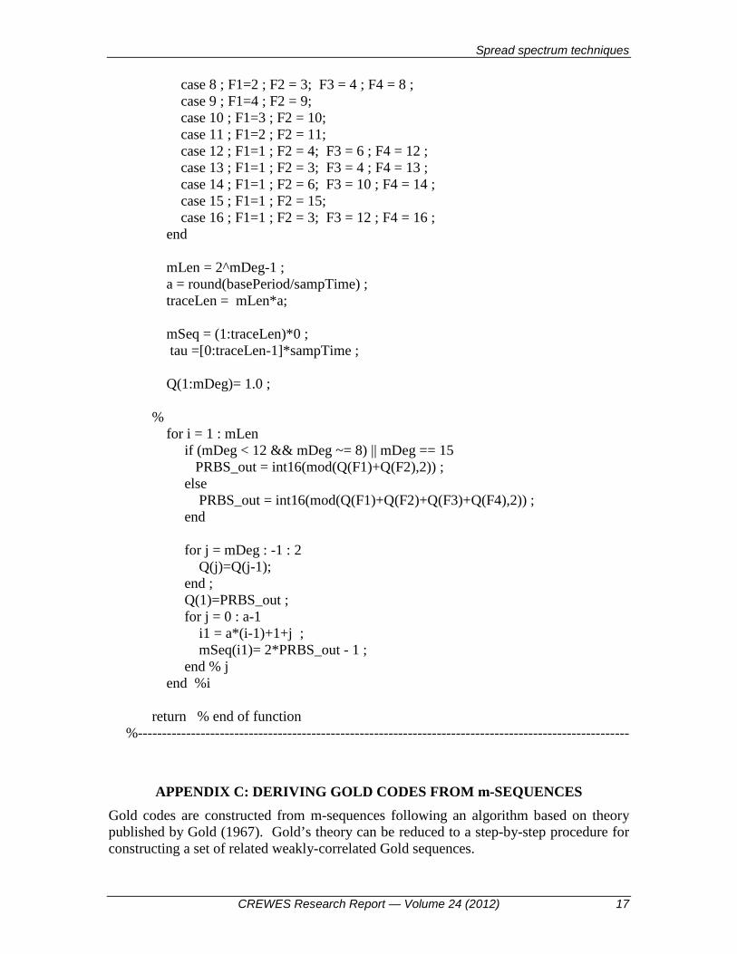
Spread spectrum techniques
CREWES Research Report — Volume 24 (2012) 17
case 8 ; F1=2 ; F2 = 3; F3 = 4 ; F4 = 8 ; case 9 ; F1=4 ; F2 = 9; case 10 ; F1=3 ; F2 = 10; case 11 ; F1=2 ; F2 = 11; case 12 ; F1=1 ; F2 = 4; F3 = 6 ; F4 = 12 ; case 13 ; F1=1 ; F2 = 3; F3 = 4 ; F4 = 13 ; case 14 ; F1=1 ; F2 = 6; F3 = 10 ; F4 = 14 ; case 15 ; F1=1 ; F2 = 15; case 16 ; F1=1 ; F2 = 3; F3 = 12 ; F4 = 16 ; end mLen = 2^mDeg-1 ; a = round(basePeriod/sampTime) ; traceLen = mLen*a; mSeq = (1:traceLen)*0 ; tau =[0:traceLen-1]*sampTime ; Q(1:mDeg)= 1.0 ; % for i = 1 : mLen if (mDeg < 12 && mDeg ~= 8) || mDeg == 15 PRBS_out = int16(mod(Q(F1)+Q(F2),2)) ; else PRBS_out = int16(mod(Q(F1)+Q(F2)+Q(F3)+Q(F4),2)) ; end for j = mDeg : -1 : 2 Q(j)=Q(j-1); end ; Q(1)=PRBS_out ; for j = 0 : a-1 i1 = a*(i-1)+1+j ; mSeq(i1)= 2*PRBS_out - 1 ; end % j end %i return % end of function
%------------------------------------------------------------------------------------------------------
APPENDIX C: DERIVING GOLD CODES FROM m-SEQUENCES Gold codes are constructed from m-sequences following an algorithm based on theory published by Gold (1967). Gold’s theory can be reduced to a step-by-step procedure for constructing a set of related weakly-correlated Gold sequences.
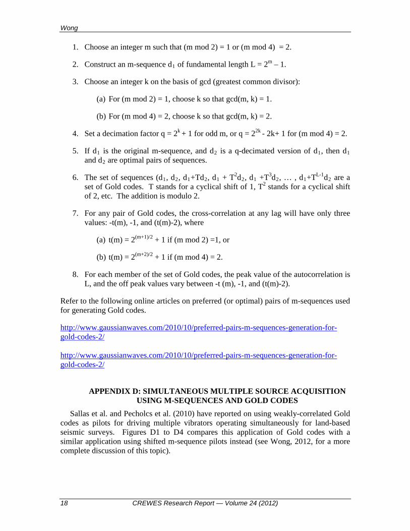
Wong
18 CREWES Research Report — Volume 24 (2012)
1. Choose an integer m such that (m mod 2) = 1 or (m mod 4) = 2.
2. Construct an m-sequence d1 of fundamental length L = 2m – 1.
3. Choose an integer k on the basis of gcd (greatest common divisor):
(a) For (m mod 2) = 1, choose k so that gcd(m, k) = 1.
(b) For (m mod 4) = 2, choose k so that gcd(m, k) = 2.
4. Set a decimation factor q = 2k + 1 for odd m, or q = 22k - 2k+ 1 for (m mod 4) = 2.
5. If d1 is the original m-sequence, and d2 is a q-decimated version of d1, then d1 and d2 are optimal pairs of sequences.
6. The set of sequences (d1, d2, d1+Td2, d1 + T2d2, d1 +T3d2, … , d1+TL-1d2 are a set of Gold codes. T stands for a cyclical shift of 1, T2 stands for a cyclical shift of 2, etc. The addition is modulo 2.
7. For any pair of Gold codes, the cross-correlation at any lag will have only three values: -t(m), -1, and (t(m)-2), where
(a) t(m) = 2(m+1)/2 + 1 if (m mod 2) =1, or
(b) t(m) = 2(m+2)/2 + 1 if (m mod 4) = 2.
8. For each member of the set of Gold codes, the peak value of the autocorrelation is L, and the off peak values vary between -t (m), -1, and (t(m)-2).
Refer to the following online articles on preferred (or optimal) pairs of m-sequences used for generating Gold codes.
http://www.gaussianwaves.com/2010/10/preferred-pairs-m-sequences-generation-for-gold-codes-2/ http://www.gaussianwaves.com/2010/10/preferred-pairs-m-sequences-generation-for-gold-codes-2/
APPENDIX D: SIMULTANEOUS MULTIPLE SOURCE ACQUISITION USING M-SEQUENCES AND GOLD CODES
Sallas et al. and Pecholcs et al. (2010) have reported on using weakly-correlated Gold codes as pilots for driving multiple vibrators operating simultaneously for land-based seismic surveys. Figures D1 to D4 compares this application of Gold codes with a similar application using shifted m-sequence pilots instead (see Wong, 2012, for a more complete discussion of this topic).

Spread spectrum techniques
CREWES Research Report — Volume 24 (2012) 19
The information presented on Figures D1 to D4 is more evidence that, due to the correlation noise which is inherent and unavoidable for Gold codes, they are less suitable for use as pilots for vibrating seismic sources than are m-sequences.
FIG. D1: Two quasi-orthogonal sets of PRBSs with m=11, L=2047, tb=4ms, ts=1ms. Full cycle periods = 8188ms; only the first 2040 ms are displayed. (a) Four shifted m-sequences; (b) four Gold codes.
On Figure D1, we show two sets of pseudorandom binary sequences, both of which are quasi-orthogonal under correlation. By quasi-orthogonal set we mean, that within each set, the autocorrelation of an individual member approximates the delta function, while the cross-correlation between two different members is nearly zero (within a restricted window of lag times).
FIG. D2: (a) Auto/cross correlations of the four shifted m-sequences on Figure D1. (b) Convolutions of wavelet with four shifted m-sequences, delayed by arrival time between four

Wong
20 CREWES Research Report — Volume 24 (2012)
sources and one receiver (R1 to R4); RT (in red) is the sum of R1 to R4 detected at the receiver. (c) Seismic traces obtained by cross-correlation of RT with each of the shifted m-sequences; (d) AGC plot of traces in (c) after removal of DC level.
FIG.: D3: (a) Auto/cross correlations of the four Gold codes on Figure D1. (b) Convolutions of wavelet with four Gold codes, delayed by arrival time between four sources and one receiver (R1 to R4); RT (in red) is the sum of R1 to R4 detected at the receiver. (c) Seismic traces obtained by cross-correlation of RT with each of the shifted m-sequences; (d) AGC plot of traces in (c).
The quasi-orthogonal nature of the set of shifted m-sequences is shown on Figure D2(a), on which the four autocorrelations of the members resemble delta functions, while the cross-correlations are very small constant values. Figure D2(b) shows the convolutions of the source function on Figure 3 with each of m-sequences on Figure D1(a). The convolutions R1 to R4 represent the received signal at a single receiver for four vibrators each driven by two cycles of a different m-sequence pilot. They have been displayed with delays and zero values that account for the travel time between a receiver and source. Since the vibrators are operating simultaneously, the total received signal RT is the sum of R1 to R4. Figure D2(c) and D2(d) shows the seismic traces reconstructed from the summed received signal RT by complete cross-correlation with each of the m-sequence pilots. The technique of driving four vibrators simultaneously with members of the quasi-orthogonal set has been successful in reconstructing the traces as if the sources were driven at non-overlapping times.
The same procedure can be applied using the set of Gold codes as pilot signals. Figure D3 (a) shows that the autocorrelations also resemble delta functions, but the cross-correlations have oscillating small non-zero values. The reconstructed seismic traces are plotted on Figure D3(d). The very weak wavelet on the original source functions is completely obscured by correlation noise. This is in sharp contrast with the traces on Figure D2(d), on which the weak wavelet appears very clearly.