Spin foams and noncommutative geometrymatilde/SpinFoamCover.pdf · SPIN FOAMS AND NONCOMMUTATIVE...
49
SPIN FOAMS AND NONCOMMUTATIVE GEOMETRY DOMENIC DENICOLA, MATILDE MARCOLLI, AND AHMAD ZAINY AL-YASRY Abstract. We extend the formalism of embedded spin networks and spin foams to in- clude topological data that encode the underlying three-manifold or four-manifold as a branched cover. These data are expressed as monodromies, in a way similar to the encoding of the gravitational field via holonomies. We then describe convolution alge- bras of spin networks and spin foams, based on the different ways in which the same topology can be realized as a branched covering via covering moves, and on possible composition operations on spin foams. We illustrate the case of the groupoid algebra of the equivalence relation determined by covering moves and a 2-semigroupoid algebra arising from a 2-category of spin foams with composition operations corresponding to a fibered product of the branched coverings and the gluing of cobordisms. The spin foam amplitudes then give rise to dynamical flows on these algebras, and the existence of low temperature equilibrium states of Gibbs form is related to questions on the existence of topological invariants of embedded graphs and embedded two-complexes with given prop- erties. We end by sketching a possible approach to combining the spin network and spin foam formalism with matter within the framework of spectral triples in noncommutative geometry. Contents 1. Introduction 2 2. Spin networks and foams enriched with topological data 3 2.1. Spin networks 3 2.2. Three-manifolds and cobordisms as branched coverings 4 2.3. Wirtinger relations 6 2.4. Covering moves for embedded graphs 7 2.5. Topologically enriched spin networks 8 2.6. Geometric covering moves 10 2.7. Spin foams and topological enrichment 13 2.8. The case of cyclic coverings 16 2.9. Embedded graphs and cobordisms 17 2.10. Geometries and topologies 18 3. Noncommutative spaces as algebras and categories 19 3.1. Algebras from categories 19 3.2. 2-categories 20 3.3. Algebras from 2-categories 21 4. A model case from arithmetic noncommutative geometry 22 4.1. Quantum statistical mechanics 22 4.2. Lattices and commensurability 23 4.3. Low temperature KMS states 24 4.4. The paradigm of emergent geometry 24 5. Categories of topspin networks and foams 25 5.1. The groupoid of topspin networks and covering moves 25 5.2. The category of topspin networks and foams 25 5.3. Including degenerate geometries 25 5.4. Representations 26 1
Transcript of Spin foams and noncommutative geometrymatilde/SpinFoamCover.pdf · SPIN FOAMS AND NONCOMMUTATIVE...
SPIN FOAMS AND NONCOMMUTATIVE GEOMETRY
DOMENIC DENICOLA, MATILDE MARCOLLI, AND AHMAD ZAINY AL-YASRY
Abstract. We extend the formalism of embedded spin networks and spin foams to in-
clude topological data that encode the underlying three-manifold or four-manifold asa branched cover. These data are expressed as monodromies, in a way similar to the
encoding of the gravitational field via holonomies. We then describe convolution alge-
bras of spin networks and spin foams, based on the different ways in which the sametopology can be realized as a branched covering via covering moves, and on possible
composition operations on spin foams. We illustrate the case of the groupoid algebra
of the equivalence relation determined by covering moves and a 2-semigroupoid algebraarising from a 2-category of spin foams with composition operations corresponding to a
fibered product of the branched coverings and the gluing of cobordisms. The spin foam
amplitudes then give rise to dynamical flows on these algebras, and the existence of lowtemperature equilibrium states of Gibbs form is related to questions on the existence of
topological invariants of embedded graphs and embedded two-complexes with given prop-
erties. We end by sketching a possible approach to combining the spin network and spinfoam formalism with matter within the framework of spectral triples in noncommutative
geometry.
Contents
1. Introduction 22. Spin networks and foams enriched with topological data 32.1. Spin networks 32.2. Three-manifolds and cobordisms as branched coverings 42.3. Wirtinger relations 62.4. Covering moves for embedded graphs 72.5. Topologically enriched spin networks 82.6. Geometric covering moves 102.7. Spin foams and topological enrichment 132.8. The case of cyclic coverings 162.9. Embedded graphs and cobordisms 172.10. Geometries and topologies 183. Noncommutative spaces as algebras and categories 193.1. Algebras from categories 193.2. 2-categories 203.3. Algebras from 2-categories 214. A model case from arithmetic noncommutative geometry 224.1. Quantum statistical mechanics 224.2. Lattices and commensurability 234.3. Low temperature KMS states 244.4. The paradigm of emergent geometry 245. Categories of topspin networks and foams 255.1. The groupoid of topspin networks and covering moves 255.2. The category of topspin networks and foams 255.3. Including degenerate geometries 255.4. Representations 26
1
2 DOMENIC DENICOLA, MATILDE MARCOLLI, AND AHMAD ZAINY AL-YASRY
5.5. Dynamics on algebras of topspin networks and foams 265.6. Equilibrium states 296. A 2-category of spin foams and fibered products 306.1. KK-classes, correspondences, and D-brane models 306.2. A 2-category of low dimensional geometries 316.3. A 2-category of topspin networks and topspin foams 326.4. The case of bicategories: loop states and spin networks 346.5. Convolution algebras of topspin networks and topspin foams 357. Topspin foams and dynamics 367.1. Dynamics from quantized area operators 377.2. More general time evolutions from spin foam amplitudes 407.3. Multiplicities in the spectrum and type II geometry 428. Spin foams with matter: almost-commutative geometries 438.1. The noncommutative geometry approach to the Standard Model 438.2. Spectral triples and loop quantum gravity 468.3. Spectral correspondences 468.4. Future work 47Acknowledgments 47References 48
1. Introduction
In this paper we extend the usual formalism of spin networks and spin foams, widely usedin the context of loop quantum gravity, to encode the additional information on the topologyof the ambient smooth three- or four-manifold, in the form of branched covering data. Inthis way, the usual data of holonomies of connections, which provide a discretization of thegravitational field in LQG models, is combined here with additional data of monodromies,which encode in a similar way the smooth topology.
The lack of uniqueness in the description of three-manifolds and four-manifolds as branchedcoverings determines an equivalence relation on the set of our topologically enriched spinnetworks and foams, which is induced by the covering moves between branch loci and mon-odromy representations. One can associate to this equivalence relation a groupoid algebra.We also consider other algebras of functions on the space of all possible spin networks andfoams with topological data, and in particular a 2-semigroupoid algebra coming from a 2-category which encodes both the usual compositions of spin foams as cobordisms betweenspin networks and a fibered product operation that parallels the KK-theory product usedin D-brane models.
The algebras obtained in this way are associative noncommutative algebras, which canbe thought of as noncommutative spaces parameterizing the collection of all topologicallyenriched spin foams and networks with the operations of composition, fibered product, orcovering moves. The lack of covering-move invariance of the spin foam amplitudes, and ofother operators such as the quantized area operator on spin networks, generates a dynamicalflow on these algebras, which in turn can be used to construct equilibrium states. Theextremal low temperature states can be seen as a way to dynamically select certain spinfoam geometries out of the parameterizing space. This approach builds on an analogy withthe algebras of Q-lattices up to commensurability arising in arithmetic noncommutativegeometry.
SPIN FOAMS AND NONCOMMUTATIVE GEOMETRY 3
2. Spin networks and foams enriched with topological data
The formalism of spin foams and spin networks was initially considered, in relation toquantum gravity, in the work of [1, 2]. It was then developed, in the context of loop quantumgravity (see [3, 4]) to provide a background-independent framework in loop quantum gravity.In the case of spin networks, the gravitational field on a three-dimensional manifold M isencoded by a graph Γ embedded in M , with representation-theoretic data attached to theedges and vertices giving the holonomies of the gravitational connection. Similarly, spinfoams represent the evolution of the gravitational field along a cobordism W between three-manifolds M and M ′; they are given by the geometric realization of a simplicial two-complexΣ embedded in W , with similar representation-theoretic data attached to the faces andedges.
In this way, spin networks give the quantum states of three-dimensional geometries, whilethe spin foams give cobordisms between spin networks and are used to define partition func-tions and transition amplitudes as “sums over histories” [3, 4]. The background indepen-dence then arises from the fact that, in this setting, one does not have to fix a backgroundmetric on M or on W , and represent the gravitational field as perturbations of this fixedmetric. One does, however, fix the background topology of M or on W .
In this section we describe a way to extend the formalism of spin networks (respectivelyspin foams) to include “topological data” as additional labeling on a graph embedded in thethree-sphere S3 (respectively, a two-complex embedded in S3×[0, 1]). These additional labelsencode the topology of a three-manifold M (respectively four-manifold W with boundary).This is achieved by representing three-manifolds and four-manifolds as branched coverings,respectively of the three-sphere or the four-sphere, branched along an embedded graph oran embedded two-complex. This means that we need only consider graphs embedded in thethree-sphere S3 and two-complexes embedded in S3 × [0, 1]; from these we obtain both thetopological information needed to construct M or W , as well as the metric information—allfrom the labeling attached to faces, edges, and vertices of these simplicial data.
In essence, while the metric information is encoded in the spin network and spin foamformalism by holonomies, the topological information will be encoded similarly by mon-odromies.
2.1. Spin networks. A spin network is the mathematical representation of the quantumstate of the gravitational field on a compact smooth three-dimensional manifold M , thoughtof as a three-dimensional hypersurface in a four-dimensional spacetime. In other words, spinnetworks should be thought of as “quantum three-geometries.” In this way, spin networksform a basis for the kinematical state space of loop quantum gravity.
Mathematically, spin networks are directed embedded graphs with edges labeled by rep-resentations of a compact Lie group, and vertices labeled by intertwiners of the adjacentedge representations. We recall the definition of spin networks given in [3].
Definition 2.1. A spin network over a compact Lie group G and embedded in a three-manifold M is a triple (Γ, ρ, ι) consisting of:
(1) an oriented graph (one-complex) Γ ⊂M ;(2) a labeling ρ of each edge e of Γ by a representation ρe of G;(3) a labeling ι of each vertex v of Γ by an intertwiner
ιv : ρe1 ⊗ · · · ⊗ ρen → ρe′1 ⊗ · · · ⊗ ρe′m ,where e1, . . . , en are the edges incoming to v and e′1, . . . , e
′m are the edges outgoing
from v.
Notice that, in the loop quantum gravity literature, often one imposes the additionalcondition that the representations ρe are irreducible. Here we take the less restrictive variant
4 DOMENIC DENICOLA, MATILDE MARCOLLI, AND AHMAD ZAINY AL-YASRY
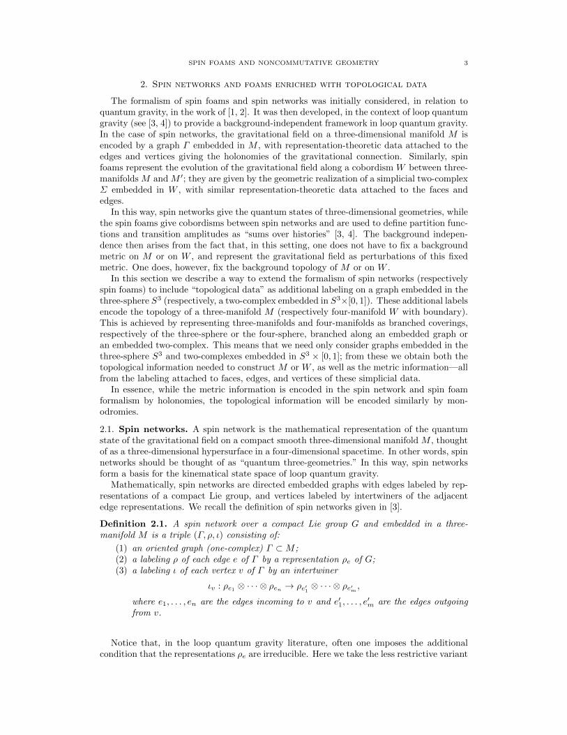
Figure 1. A sample spin network, labeled with representations of SU(2)
used in the physics literature, and we do not require irreducibility. Another point wherethere are different variants in the loop quantum gravity literature is whether the graphs Γshould be regarded as combinatorial objects or as spatial graphs embedded in a specifiedthree-manifold. We adopt here the convention of regarding graphs as embedded. This will becrucial in order to introduce the additional monodromy data that determine the underlyingthree-manifold topology, as we discuss at length in the following sections.
We can intuitively connect this to a picture of a quantum three-geometry as follows [4].We think of such a geometry as a set of “grains of space,” some of which are adjacent toothers. Then, each vertex of the spin network corresponds to a grain of space, while eachedge corresponds to the surfaces separating two adjacent grains. The quantum state is thencharacterized by the quantum numbers given in our collections ρ and ι: in fact, the labelιv determines the quantum number of a grain’s volume, while the label ρe determines thequantum number of the area of a separating surface. The area operator and its role in ourresults is is discussed further in section 7.1.
The Hilbert space of quantum states associated to spin networks is spanned by the ambientisotopy classes of embedded graphs Γ ⊂M , with labels of edges and vertices as above; see [4]for more details. In fact, for embedded graphs, as well as for knots and links, being relatedby ambient isotopy is the same as being related by an orientation-preserving piecewise-linearhomeomorphic change of coordinates in the ambient S3, so that is the natural equivalencerelation one wants to impose in the quantum gravity setting.
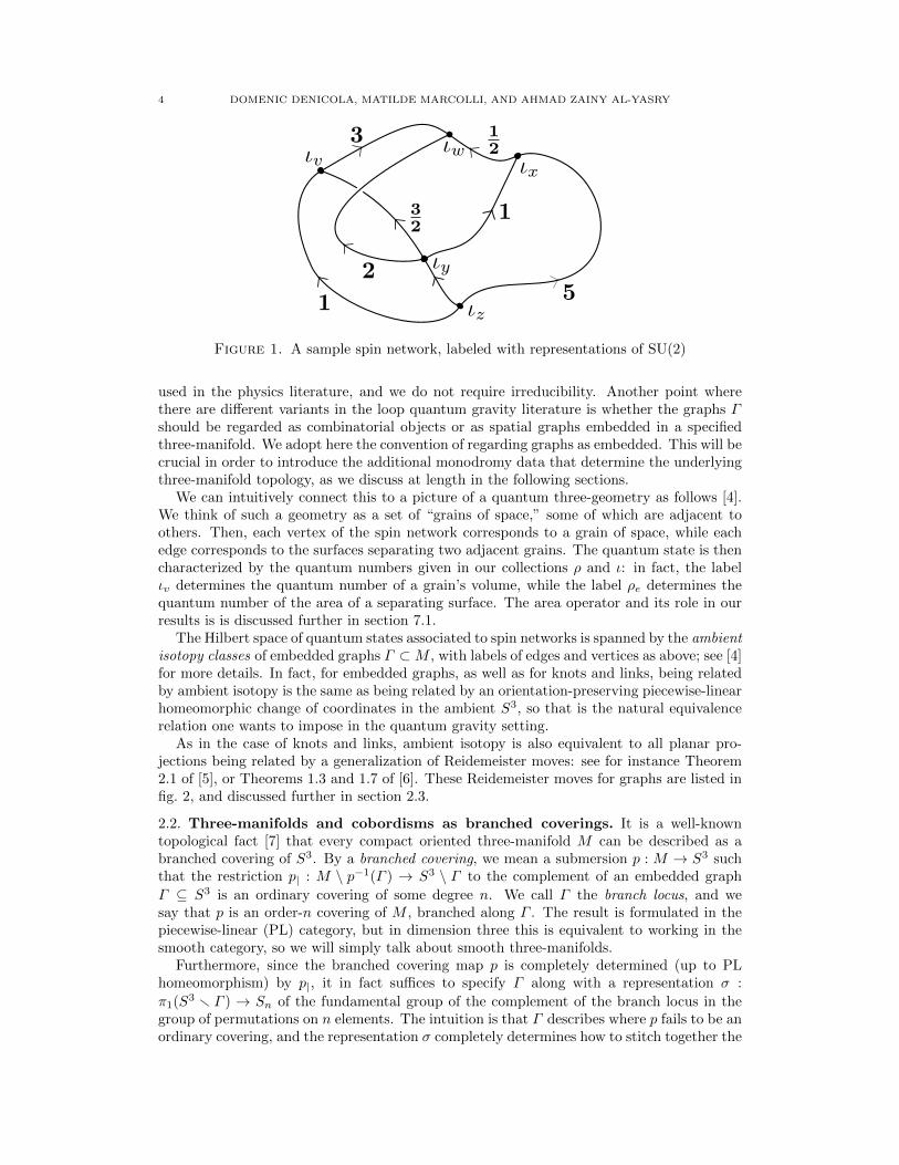
As in the case of knots and links, ambient isotopy is also equivalent to all planar pro-jections being related by a generalization of Reidemeister moves: see for instance Theorem2.1 of [5], or Theorems 1.3 and 1.7 of [6]. These Reidemeister moves for graphs are listed infig. 2, and discussed further in section 2.3.
2.2. Three-manifolds and cobordisms as branched coverings. It is a well-knowntopological fact [7] that every compact oriented three-manifold M can be described as abranched covering of S3. By a branched covering, we mean a submersion p : M → S3 suchthat the restriction p| : M \ p−1(Γ ) → S3 \ Γ to the complement of an embedded graph
Γ ⊆ S3 is an ordinary covering of some degree n. We call Γ the branch locus, and wesay that p is an order-n covering of M , branched along Γ . The result is formulated in thepiecewise-linear (PL) category, but in dimension three this is equivalent to working in thesmooth category, so we will simply talk about smooth three-manifolds.
Furthermore, since the branched covering map p is completely determined (up to PLhomeomorphism) by p|, it in fact suffices to specify Γ along with a representation σ :
π1(S3 r Γ ) → Sn of the fundamental group of the complement of the branch locus in thegroup of permutations on n elements. The intuition is that Γ describes where p fails to be anordinary covering, and the representation σ completely determines how to stitch together the
SPIN FOAMS AND NONCOMMUTATIVE GEOMETRY 5KHOVANOV HOMOLOGY AND EMBEDDED GRAPHS 13
1!
2!
3!
4!
5!
FIGURE 9. Generalized Reidemeister moves by Kauffman
FIGURE 10. local replacement to a vertex in the graph G
Figure 2. Reidemeister moves for embedded graphs
different branches of the covering over the branch locus [7, 8]. The use of the fundamentalgroup of the complement implies that the embedding of Γ in S3 is important: that is, it isnot only the structure of Γ as an abstract combinatorial graph that matters.
Notably, the correspondence between three-manifolds and branched coverings of the three-sphere is not bijective: in general for a given manifold there will be multiple pairs (Γ, σ)that realize it as a branched covering. The conditions for two pairs (Γ, σ) and (Γ ′, σ′) ofbranching loci and fundamental group representations to give rise to the same three-manifold(up to PL homeomorphism) are discussed further in section 2.4.
As an example of this lack of uniqueness phenomenon, the Poincare homology sphere Mcan be viewed as a fivefold covering of S3 branched along the trefoil K2,3, or as a threefoldcovering branched along the (2, 5) torus knot K2,5, among others [9].
There is a refinement of the branched covering description of three-manifolds, the Hilden–Montesinos theorem [10, 11], which shows that one can in fact always realize three-manifoldsas threefold branched coverings of S3, branched along a knot. Although this result is muchstronger, for our quantum gravity applications it is preferable to work with the weakerstatement given above, with branch loci that are embedded graphs and arbitrary order ofcovering. We comment further in section 6.4 on the case of coverings branched along knotsor links.
Another topological result we will be using substantially in the following is the analogousbranched covering description for four-manifolds, according to which all compact PL four-manifolds can be realized as branched coverings of the four-sphere S4, branched along anembedded simplicial two-complex. In this case also one has a stronger result [12], accordingto which one can always realize the PL four-manifolds as fourfold coverings of S4 branchedalong an embedded surface. However, as in the case of three-manifolds, we work with themore general and weaker statement that allows for coverings of arbitrary order, along anembedded two-complex as the branch locus. Using the fact that in dimension four there isagain no substantial difference between the PL and the smooth category, in the followingwe work directly with smooth four-manifolds.
6 DOMENIC DENICOLA, MATILDE MARCOLLI, AND AHMAD ZAINY AL-YASRY
In the setting of loop quantum gravity, where one views spin networks as elements ofan algebra of functions of the connection, the product of spin networks is well behaved inthe piecewise analytic rather than in the smooth setting, due to the way in which edges ofdifferent graphs can intersect. A formulation can be given also in PL setting, as in [13, 14].The setting we consider here will then be very closely related to the PL version of [14].
We also recall here the notion of branched cover cobordism between three-manifolds real-ized as branched coverings of S3. We use the same terminology as in [15].
First consider three-manifolds M0 and M1, each realized as a branched covering pi :Mi → S3 branched along embedded graphs Γi ⊂ S3. Then a branched cover cobordism isa smooth four-manifold W with boundary ∂W = M0 ∪ M1 and with a branched coveringmap q : W → S3 × [0, 1], branched along an embedded two-complex Σ ⊂ S3 × [0, 1], withthe property that ∂Σ = Γ0 ∪ Γ1 and the restrictions of the covering map q to S3 × {0} andS3 × {1} agree with the covering maps p0 and p1, respectively.
For the purpose of the 2-category construction we present later in the paper, we alsoconsider cobordisms W that are realized in two different ways as branched cover cobordismsbetween three-manifolds, as described in [15]. This version will be used as a form of geometriccorrespondences providing the 2-morphisms of our 2-category.
To illustrate this latter concept, let M0 and M1 be two closed smooth three-manifolds,each realized in two ways as a branched covering of S3 via respective branchings over em-bedded graphs Γi and Γ ′i for i ∈ {0, 1}. We represent this with the notation
Γi ⊂ S3 pi←Mip′i→ S3 ⊃ Γ ′i .
A branched cover cobordism W between M0 and M1 is a smooth four-dimensional manifoldwith boundary ∂W = M0∪M1, which is realized in two ways as a branched cover cobordismof S3×[0, 1] branched along two-complexes Σ and Σ′ embedded in S3×[0, 1], with respectiveboundaries ∂Σ = Σ ∩ (S3 × {0, 1}) = Γ0 ∪ Γ1 and ∂Σ′ = Γ ′0 ∪ Γ ′1. We represent this with asimilar notation,
Σ ⊂ S3 × [0, 1]q←W
q′→ S3 × [0, 1] ⊃ Σ′.The covering maps q and q′ have the property that their restrictions to S3×{0} agree withthe maps p0 and p′0, respectively, while their restrictions to S3 × {1} agree with the mapsp1 and p′1.
2.3. Wirtinger relations. As we mentioned in the previous section, a branched coveringp : M → S3, branched along an embedded graph Γ , is completely determined by a grouprepresentation σ : π1(S3 r Γ ) → Sn. Here we pause to note that the fundamental groupπ1(S3 r Γ ) of the complement of an embedded graph in the three-sphere has an explicitpresentation, which is very similar to the usual Wirtinger presentation for the fundamentalgroup of knot complements.
The advantage of describing the representation σ in terms of an explicit presentation isthat it will allow us to encode the data of the branched covering p : M → S3 completelyin terms of labels attached to edges of a planar projection of the graph, with relations atvertices and crossings in the planar diagram. Furthermore, if two embedded graphs Γ andΓ ′ in S3 are ambient-isotopic, then any given planar diagrams D(Γ ) and D(Γ ′) differ by afinite sequence of moves that generalize to graphs the usual Reidemeister moves for knotsand links, as shown in fig. 2. (For more details, see Theorem 2.1 of [5] and Theorem 1.7 of[6].)
For the rest of this discussion, we use the following terminology. An undercrossing in aplanar diagram is the line that passes underneath at a crossing, while an overcrossing is theline that passes above the other. Thus an arc of a planar diagram D(Γ ) is either an edgeof the graph Γ , if the edge does not appear as an undercrossing in the diagram, or a halfedge of Γ , when the corresponding edge is an undercrossing. Thus, an edge of Γ alwayscorresponds to a number N + 1 of arcs in D(Γ ), where N is the number of undercrossings
SPIN FOAMS AND NONCOMMUTATIVE GEOMETRY 7
that edge exhibits in the planar diagram D(Γ ). The following result is well known, but werecall it here for convenience.
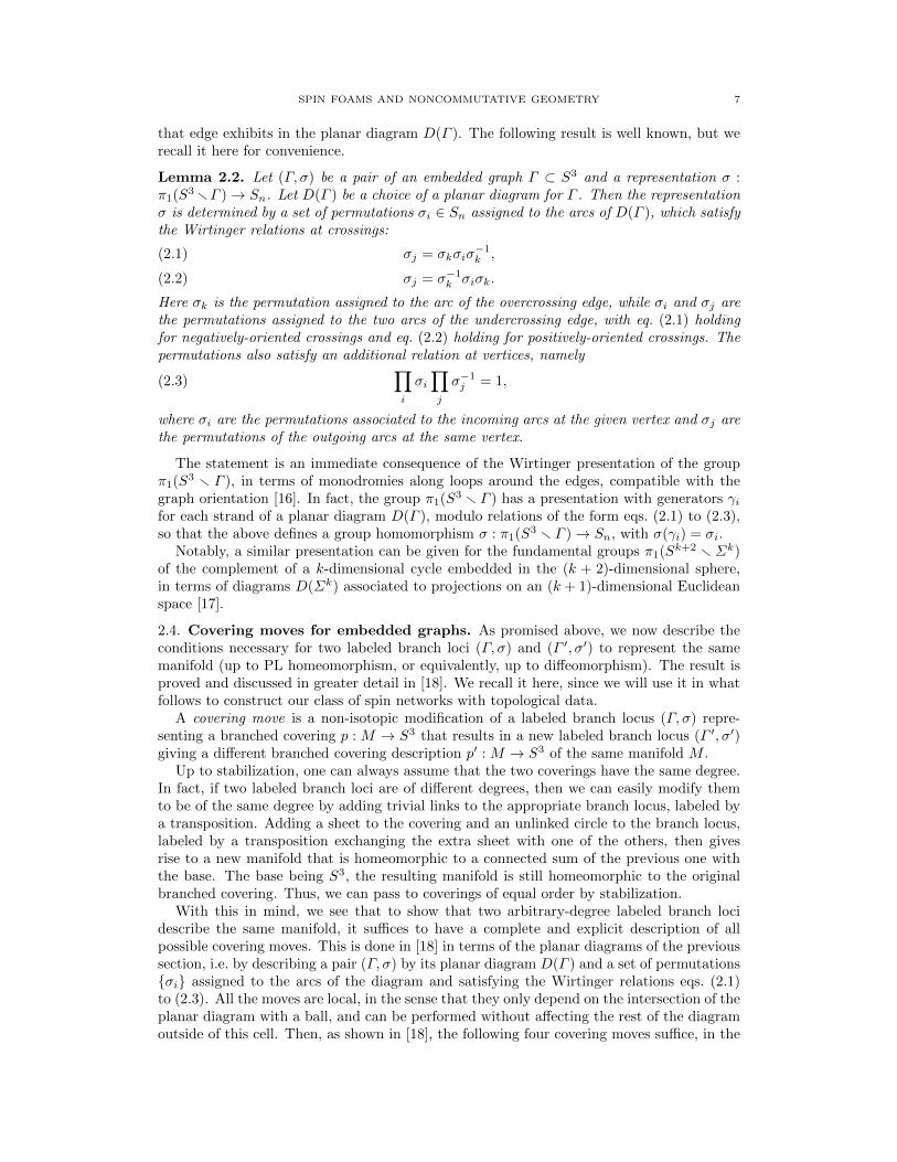
Lemma 2.2. Let (Γ, σ) be a pair of an embedded graph Γ ⊂ S3 and a representation σ :π1(S3 rΓ )→ Sn. Let D(Γ ) be a choice of a planar diagram for Γ . Then the representationσ is determined by a set of permutations σi ∈ Sn assigned to the arcs of D(Γ ), which satisfythe Wirtinger relations at crossings:
σj = σkσiσ−1k ,(2.1)
σj = σ−1k σiσk.(2.2)
Here σk is the permutation assigned to the arc of the overcrossing edge, while σi and σj arethe permutations assigned to the two arcs of the undercrossing edge, with eq. (2.1) holdingfor negatively-oriented crossings and eq. (2.2) holding for positively-oriented crossings. Thepermutations also satisfy an additional relation at vertices, namely
(2.3)∏i
σi∏j
σ−1j = 1,
where σi are the permutations associated to the incoming arcs at the given vertex and σj arethe permutations of the outgoing arcs at the same vertex.
The statement is an immediate consequence of the Wirtinger presentation of the groupπ1(S3 r Γ ), in terms of monodromies along loops around the edges, compatible with thegraph orientation [16]. In fact, the group π1(S3 r Γ ) has a presentation with generators γifor each strand of a planar diagram D(Γ ), modulo relations of the form eqs. (2.1) to (2.3),so that the above defines a group homomorphism σ : π1(S3 r Γ )→ Sn, with σ(γi) = σi.
Notably, a similar presentation can be given for the fundamental groups π1(Sk+2 rΣk)of the complement of a k-dimensional cycle embedded in the (k + 2)-dimensional sphere,in terms of diagrams D(Σk) associated to projections on an (k + 1)-dimensional Euclideanspace [17].
2.4. Covering moves for embedded graphs. As promised above, we now describe theconditions necessary for two labeled branch loci (Γ, σ) and (Γ ′, σ′) to represent the samemanifold (up to PL homeomorphism, or equivalently, up to diffeomorphism). The result isproved and discussed in greater detail in [18]. We recall it here, since we will use it in whatfollows to construct our class of spin networks with topological data.
A covering move is a non-isotopic modification of a labeled branch locus (Γ, σ) repre-senting a branched covering p : M → S3 that results in a new labeled branch locus (Γ ′, σ′)giving a different branched covering description p′ : M → S3 of the same manifold M .
Up to stabilization, one can always assume that the two coverings have the same degree.In fact, if two labeled branch loci are of different degrees, then we can easily modify themto be of the same degree by adding trivial links to the appropriate branch locus, labeled bya transposition. Adding a sheet to the covering and an unlinked circle to the branch locus,labeled by a transposition exchanging the extra sheet with one of the others, then givesrise to a new manifold that is homeomorphic to a connected sum of the previous one withthe base. The base being S3, the resulting manifold is still homeomorphic to the originalbranched covering. Thus, we can pass to coverings of equal order by stabilization.
With this in mind, we see that to show that two arbitrary-degree labeled branch locidescribe the same manifold, it suffices to have a complete and explicit description of allpossible covering moves. This is done in [18] in terms of the planar diagrams of the previoussection, i.e. by describing a pair (Γ, σ) by its planar diagram D(Γ ) and a set of permutations{σi} assigned to the arcs of the diagram and satisfying the Wirtinger relations eqs. (2.1)to (2.3). All the moves are local, in the sense that they only depend on the intersection of theplanar diagram with a ball, and can be performed without affecting the rest of the diagramoutside of this cell. Then, as shown in [18], the following four covering moves suffice, in the
8 DOMENIC DENICOLA, MATILDE MARCOLLI, AND AHMAD ZAINY AL-YASRY
sense that any two diagrams giving rise to the same three-manifold can be related by a finitesequence of these moves (after stabilization).
V1!
V2!
(a) At vertices
C1!
C2!
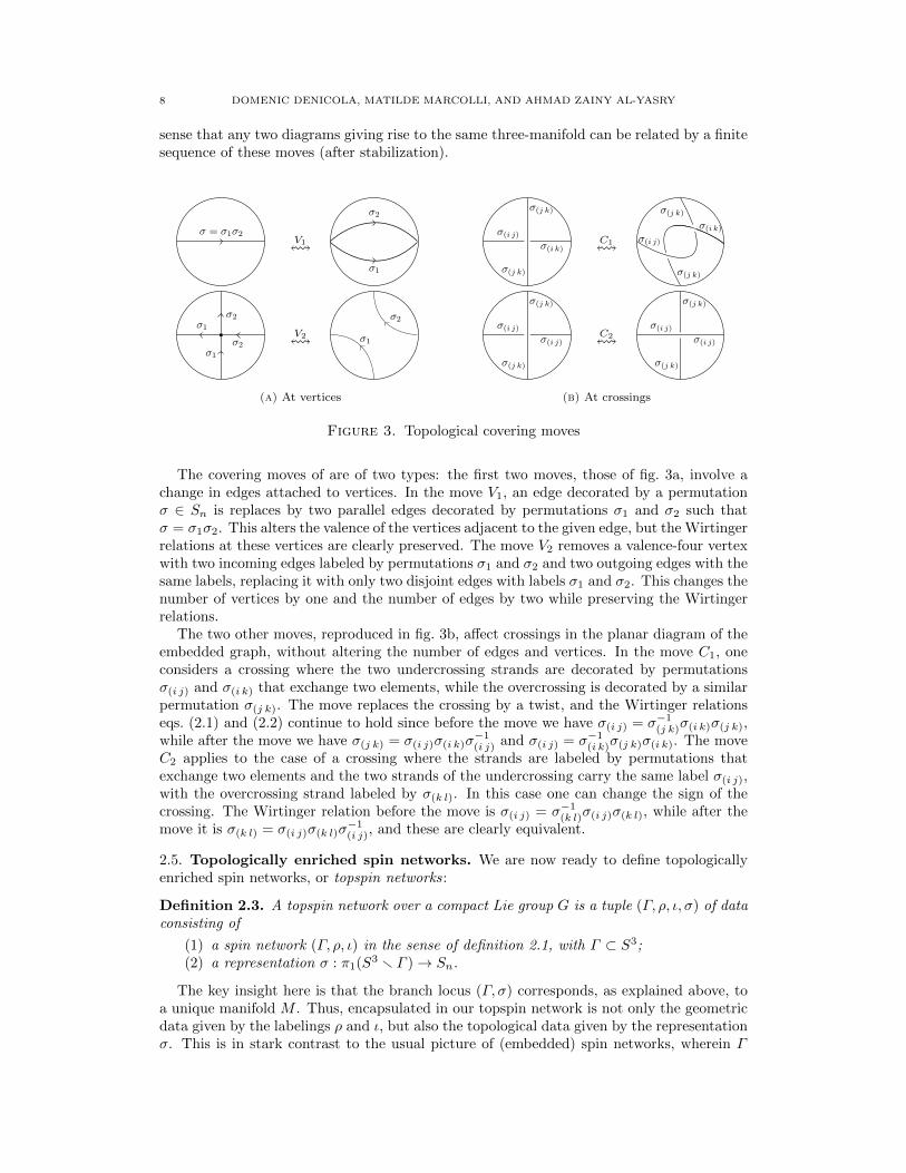
(b) At crossings
Figure 3. Topological covering moves
The covering moves of are of two types: the first two moves, those of fig. 3a, involve achange in edges attached to vertices. In the move V1, an edge decorated by a permutationσ ∈ Sn is replaces by two parallel edges decorated by permutations σ1 and σ2 such thatσ = σ1σ2. This alters the valence of the vertices adjacent to the given edge, but the Wirtingerrelations at these vertices are clearly preserved. The move V2 removes a valence-four vertexwith two incoming edges labeled by permutations σ1 and σ2 and two outgoing edges with thesame labels, replacing it with only two disjoint edges with labels σ1 and σ2. This changes thenumber of vertices by one and the number of edges by two while preserving the Wirtingerrelations.
The two other moves, reproduced in fig. 3b, affect crossings in the planar diagram of theembedded graph, without altering the number of edges and vertices. In the move C1, oneconsiders a crossing where the two undercrossing strands are decorated by permutationsσ(i j) and σ(i k) that exchange two elements, while the overcrossing is decorated by a similarpermutation σ(j k). The move replaces the crossing by a twist, and the Wirtinger relationseqs. (2.1) and (2.2) continue to hold since before the move we have σ(i j) = σ−1
(j k)σ(i k)σ(j k),while after the move we have σ(j k) = σ(i j)σ(i k)σ
−1(i j) and σ(i j) = σ−1
(i k)σ(j k)σ(i k). The moveC2 applies to the case of a crossing where the strands are labeled by permutations thatexchange two elements and the two strands of the undercrossing carry the same label σ(i j),with the overcrossing strand labeled by σ(k l). In this case one can change the sign of thecrossing. The Wirtinger relation before the move is σ(i j) = σ−1
(k l)σ(i j)σ(k l), while after themove it is σ(k l) = σ(i j)σ(k l)σ
−1(i j), and these are clearly equivalent.
2.5. Topologically enriched spin networks. We are now ready to define topologicallyenriched spin networks, or topspin networks:
Definition 2.3. A topspin network over a compact Lie group G is a tuple (Γ, ρ, ι, σ) of dataconsisting of
(1) a spin network (Γ, ρ, ι) in the sense of definition 2.1, with Γ ⊂ S3;(2) a representation σ : π1(S3 r Γ )→ Sn.
The key insight here is that the branch locus (Γ, σ) corresponds, as explained above, toa unique manifold M . Thus, encapsulated in our topspin network is not only the geometricdata given by the labelings ρ and ι, but also the topological data given by the representationσ. This is in stark contrast to the usual picture of (embedded) spin networks, wherein Γ
SPIN FOAMS AND NONCOMMUTATIVE GEOMETRY 9
is a graph embedded into a specific manifold M with fixed topology, and thus only givesgeometrical data on the gravitational field.
The data of a topspin network can equivalently be described in terms of planar projectionsD(Γ ) of the embedded graph Γ ⊂ S3, decorated with labels ρi and σi on the strands of thediagram, where the ρi are the representations of G associated to the corresponding edgesof the graph Γ and σi ∈ Sn are permutations satisfying the Wirtinger relations eqs. (2.1)to (2.3). The vertices of the diagram D(Γ ) are decorated with the intertwiners ιv.
It is customary in the setting of loop quantum gravity to take graphs Γ that arise fromtriangulations of three-manifolds and form directed systems associated to families of nestedgraphs, such as barycentric subdivisions of a triangulation. One often describes quantumoperators in terms of direct limits over such families [4].
In the setting of topspin networks described here, one can start from a graph Γ which is,for instance, a triangulation of the three-sphere S3, which contains as a subgraph Γ ′ ⊂ Γthe branch locus of a branched covering describing a three-manifold M . By pullback, oneobtains from it a triangulation of the three-manifold M . Viewed as a topspin network, thediagrams D(Γ ) will carry nontrivial topological labels σi on the strands belonging to thesubdiagram D(Γ ′) while the strands in the rest of the diagram are decorated with σi = 1;all the strands can carry nontrivial ρi. In the case of a barycentric subdivision, the newedges belonging to the same edge before subdivision maintain the same labels σi, while thenew edges in the barycentric subdivision that do not come from edges of the previous graphcarry trivial topological labels. Thus, all the arguments usually carried out in terms of directlimits and nested subgraphs can be adapted to the case of topspin networks without change.Working with data of graphs Γ containing the branch locus Γ ′ as a subgraph is also verynatural in terms of the fibered product composition we describe in section 6, based on theconstruction of [15].
Also in loop quantum gravity, one considers a Hilbert space generated by the spin networks[4], where the embedded graphs are taken up to ambient isotopy, or equivalently up to a PLchange of coordinates in the ambient S3. (We deal here only with spin networks embeddedin S3, since as explained above this is sufficiently general after we add the topological dataσ.) This can be extended to a Hilbert space H of topspin networks by requiring that twotopspin networks are orthogonal if they are not describing the same three-manifold, thatis, if they are not related (after stabilization) by covering moves, and by defining the innerproduct 〈ψ,ψ′〉 of topspin networks that are equivalent under covering moves to be the usualinner product of the underlying spin networks obtained by forgetting the presence of theadditional topological data σ, σ′.
It is natural to ask whether, given a 3-manifold M and a spin network Ψ = (Γ, ρ, ι) inM , there exists always a (non-unique) topspin network Ψ ′ = (Γ ′, ρ′, ι′, σ′) in S3 from whichboth M and Γ can be recovered. One way to achieve this is to choose a realization of M asa branched covering of S3, branched along a locus Γ ′′ and consider then the image graphp(Γ ) under the projection p : M → S3. This will intersect Γ ′′ along a (possibly empty)subgraph. For simplicity let us consider the case where they do not intersect and where Γis contained inside a fundamental domain of the action of the group of deck transformationsof the covering p : M r p−1(Γ ′′) → S3 r Γ ′′. One considers then the topspin networkΨ ′ = (Γ ′, ρ′, ι′, σ′) where Γ ′ = p(Γ ) ∪ Γ ′′, with the topological labels on Γ ′′ that determinethe branched cover p : M → S3 and trivial on p(Γ ), and with the labels (ρ′, ι′) on p(Γ )that agree with the corresponding labels (ρ, ι) on Γ , extended trivially to Γ ′′. Notice,however, that the preimage under the projection p of Γ ′ contains a number of copies ofgraphs isomorphic to Γ equal to the order of the covering. Thus, one recovers the originalspin network Ψ but with a multiplicity factor and with an additional component p−1(Γ ′′),which, however, carries no information in M and can be discarded.
10 DOMENIC DENICOLA, MATILDE MARCOLLI, AND AHMAD ZAINY AL-YASRY
2.6. Geometric covering moves. The addition of topological data σ to spin networks,on top of the preexisting geometric labelings ρ and ι, necessitates that we ensure these twotypes of data are compatible. The essential issue is the previously-discussed fact that agiven three-manifold M can have multiple descriptions as a labeled branch locus, say asboth (Γ, σ) and (Γ ′, σ′). If (Γ, ρ, ι, σ) is a topspin network representing a certain geometricconfiguration over M , then we would like to be able to say when another topspin network(Γ ′, ρ′, ι′, σ′), also corresponding to the manifold M via the data (Γ ′, σ′), represents thesame geometric configuration. That is, what are the conditions relating ρ′ and ι′ to ρ and ιthat ensure geometric equivalence?
Since (Γ, σ) and (Γ ′, σ′) represent the same manifold, they can be related by the coveringmoves of section 2.4. These covering moves can be interpreted as answering the question “ifone makes a local change to the graph, how must the topological labeling change?” In thissection, our task is to answer a very similar question, namely, “if one makes a local changeto the graph, how must the geometric labeling change?” Phrased this way, it is easy to seethat we simply need to give an account of what happens to the geometric labelings underthe same covering moves as before.
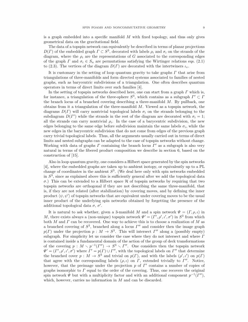
The first thing to note is that, since in definition 2.3 we do not demand that the edge-labels are given by irreducible representations, there is a certain type of trivial equivalencebetween different geometric labelings that emerges. To see this, consider the following twovery simple spin networks:
vs.
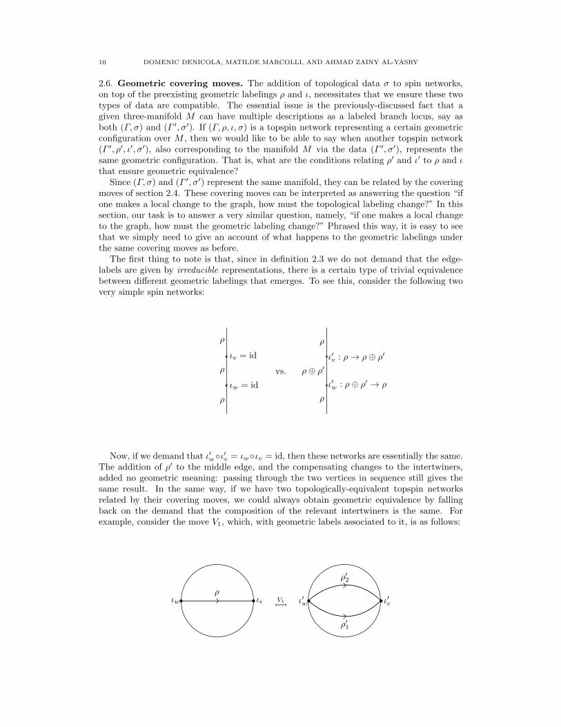
Now, if we demand that ι′w◦ι′v = ιw◦ιv = id, then these networks are essentially the same.The addition of ρ′ to the middle edge, and the compensating changes to the intertwiners,added no geometric meaning: passing through the two vertices in sequence still gives thesame result. In the same way, if we have two topologically-equivalent topspin networksrelated by their covering moves, we could always obtain geometric equivalence by fallingback on the demand that the composition of the relevant intertwiners is the same. Forexample, consider the move V1, which, with geometric labels associated to it, is as follows:
V1!
SPIN FOAMS AND NONCOMMUTATIVE GEOMETRY 11
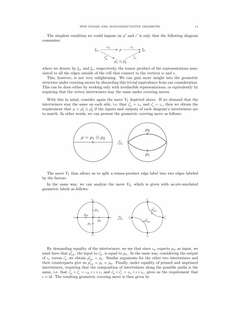
The simplest condition we could impose on ρ′ and ι′ is only that the following diagramcommutes:
ξwιw - ρ
ιe - ξe
ρ′1 ⊗ ρ′2ι′e
-ι ′w
-
where we denote by ξw and ξe, respectively, the tensor product of the representations asso-ciated to all the edges outside of the cell that connect to the vertices w and e.
This, however, is not very enlightening. We can gain more insight into the geometricstructure under covering moves by discarding this trivial equivalence from our consideration.This can be done either by working only with irreducible representations, or equivalently byrequiring that the vertex intertwiners stay the same under covering moves.
With this in mind, consider again the move V1 depicted above. If we demand that theintertwiners stay the same on each side, i.e. that ι′w = ιw and ι′e = ιe, then we obtain therequirement that ρ = ρ′1 ⊗ ρ′2 if the inputs and outputs of each diagram’s intertwiners areto match. In other words, we can present the geometric covering move as follows:
V1!
The move V1 thus allows us to split a tensor-product edge label into two edges labeledby the factors.
In the same way, we can analyze the move V2, which is given with as-yet-unrelatedgeometric labels as follows:
V2!
By demanding equality of the intertwiners, we see that since ιw expects ρw as input, wemust have that ρ′sw, the input to ι′w, is equal to ρw. In the same way, considering the outputof ιs versus ι′s, we obtain ρ′sw = ρs. Similar arguments for the other two intertwiners andtheir counterparts give us ρ′en = ρe = ρn. Finally, under equality of primed and unprimedintertwiners, requiring that the composition of intertwiners along the possible paths is thesame, i.e. that ι′w ◦ ι′s = ιw ◦ ι ◦ ιs and ι′n ◦ ι′e = ιn ◦ ι ◦ ιe, gives us the requirement thatι = id. The resulting geometric covering move is then given by
12 DOMENIC DENICOLA, MATILDE MARCOLLI, AND AHMAD ZAINY AL-YASRY
V2!
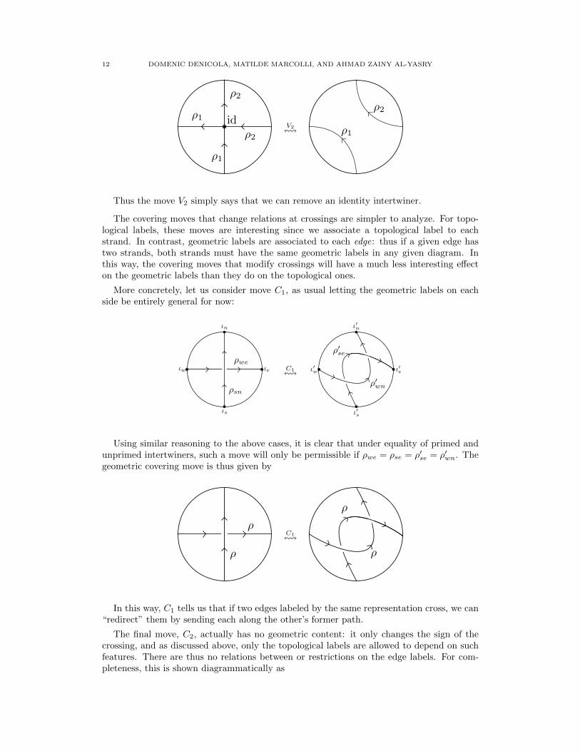
Thus the move V2 simply says that we can remove an identity intertwiner.
The covering moves that change relations at crossings are simpler to analyze. For topo-logical labels, these moves are interesting since we associate a topological label to eachstrand. In contrast, geometric labels are associated to each edge: thus if a given edge hastwo strands, both strands must have the same geometric labels in any given diagram. Inthis way, the covering moves that modify crossings will have a much less interesting effecton the geometric labels than they do on the topological ones.
More concretely, let us consider move C1, as usual letting the geometric labels on eachside be entirely general for now:
C1!
Using similar reasoning to the above cases, it is clear that under equality of primed andunprimed intertwiners, such a move will only be permissible if ρwe = ρse = ρ′se = ρ′wn. Thegeometric covering move is thus given by
C1!
In this way, C1 tells us that if two edges labeled by the same representation cross, we can“redirect” them by sending each along the other’s former path.
The final move, C2, actually has no geometric content: it only changes the sign of thecrossing, and as discussed above, only the topological labels are allowed to depend on suchfeatures. There are thus no relations between or restrictions on the edge labels. For com-pleteness, this is shown diagrammatically as
SPIN FOAMS AND NONCOMMUTATIVE GEOMETRY 13
C1!
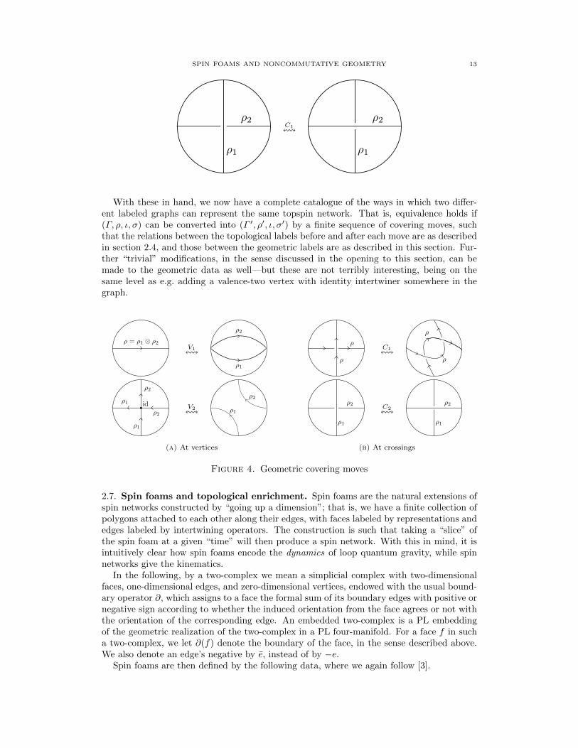
With these in hand, we now have a complete catalogue of the ways in which two differ-ent labeled graphs can represent the same topspin network. That is, equivalence holds if(Γ, ρ, ι, σ) can be converted into (Γ ′, ρ′, ι, σ′) by a finite sequence of covering moves, suchthat the relations between the topological labels before and after each move are as describedin section 2.4, and those between the geometric labels are as described in this section. Fur-ther “trivial” modifications, in the sense discussed in the opening to this section, can bemade to the geometric data as well—but these are not terribly interesting, being on thesame level as e.g. adding a valence-two vertex with identity intertwiner somewhere in thegraph.
V1!
V2!
(a) At vertices
C1!
C2!
(b) At crossings
Figure 4. Geometric covering moves
2.7. Spin foams and topological enrichment. Spin foams are the natural extensions ofspin networks constructed by “going up a dimension”; that is, we have a finite collection ofpolygons attached to each other along their edges, with faces labeled by representations andedges labeled by intertwining operators. The construction is such that taking a “slice” ofthe spin foam at a given “time” will then produce a spin network. With this in mind, it isintuitively clear how spin foams encode the dynamics of loop quantum gravity, while spinnetworks give the kinematics.
In the following, by a two-complex we mean a simplicial complex with two-dimensionalfaces, one-dimensional edges, and zero-dimensional vertices, endowed with the usual bound-ary operator ∂, which assigns to a face the formal sum of its boundary edges with positive ornegative sign according to whether the induced orientation from the face agrees or not withthe orientation of the corresponding edge. An embedded two-complex is a PL embeddingof the geometric realization of the two-complex in a PL four-manifold. For a face f in sucha two-complex, we let ∂(f) denote the boundary of the face, in the sense described above.We also denote an edge’s negative by e, instead of by −e.
Spin foams are then defined by the following data, where we again follow [3].
14 DOMENIC DENICOLA, MATILDE MARCOLLI, AND AHMAD ZAINY AL-YASRY
Definition 2.4. Suppose that ψ = (Γ, ρ, ι) and ψ′ = (Γ ′, ρ′, ι′) are spin networks over G,with the graphs Γ and Γ ′ embedded in three-manifolds M and M ′, respectively. A spin foamΨ : ψ → ψ′ embedded in a cobordism W with ∂W = M ∪ M ′ is then a triple Ψ = (Σ, ρ, ι)consisting of:
(1) an oriented two-complex Σ ⊆W , such that Γ ∪ Γ ′ borders Σ: that is, ∂Σ = Γ ∪ Γ ′,and there exist cylinder neighborhoods Mε = M × [0, ε) and M ′ε = M ′ × (−ε, 0] inW such that Σ ∩Mε = Γ × [0, ε) and Σ ∩ M ′ε = Γ ′ × (−ε, 0];
(2) a labeling ρ of each face f of Σ by a representation ρf of G;(3) a labeling ι of each edge e of Σ that does not lie in Γ or Γ ′ by an intertwiner
ιe :⊗
f :e∈∂(f)
ρf →⊗
f ′:e∈∂(f ′)
ρf ′
with the additional consistency conditions
(1) for any edge e in Γ , letting fe be the face in Σ ∩Mε bordered by e, we must havethat ρfe = (ρe)
∗ if e ∈ ∂(fe), or ρfe = ρe if e ∈ ∂(fe);(2) for any vertex v of Γ , letting ev be the edge in Σ ∩Mε adjacent to v, we must have
that ιev = ιv after appropriate dualizations to account for the different orientationsof faces and edges as above;
(3) dual conditions must hold for edges and vertices from Γ ′ and faces and edges inΣ ∩M ′ε, i.e. we would have ρfe = ρe if e ∈ ∂(fe) and ρfe = (ρe)
∗ if e ∈ ∂(fe), andlikewise for vertices.
Thus, spin foams are cobordisms between spin networks, with compatible labeling of theedges, vertices, and faces. They represent quantized four-dimensional geometries inside afixed smooth four-manifold W .
Notice that, in the context of spin foams, there are some variants regarding what no-tion of cobordisms between embedded graphs one considers. A more detailed discussion ofcobordisms of embedded graphs is given in section 2.9 below.
When working with topspin networks, one can correspondingly modify the notion of spinfoams to provide cobordisms compatible with the topological data, in such a way that oneno longer has to specify the four-manifold W with ∂W = M ∪ M ′ in advance: one can workwith two-complexes Σ embedded in the trivial cobordism S3× [0, 1] and the topology of Wis encoded as part of the data of a topspin foam, just as the three-manifolds M and M ′ areencoded in their respective topspin networks.
In the following we say that a three-manifold M corresponds to (Γ, σ) if it is the branchedcover of S3 determined by the representation σ : π1(S3 rΓ )→ Sn, and similarly for a four-manifold W corresponding to data (Σ, σ).
Definition 2.5. Suppose that ψ = (Γ, ρ, ι, σ) and ψ′ = (Γ ′, ρ′, ι′, σ′) are topspin networksover G, with topological labels in the same permutation group Sn and with Γ, Γ ′ ⊂ S3. Atopspin foam Ψ : ψ → ψ′ over G is a tuple Ψ = (Σ, ρ, ι, σ) of data consisting of
(1) a spin foam (Σ, ρ, ι) between ψ and ψ′ in the sense of definition 2.4, with Σ ⊂S3 × [0, 1];
(2) a representation σ : π1((S3 × [0, 1]) r Σ) → Sn, such that the manifold W corre-sponding to the labeled branch locus (Σ, σ) is a branched cover cobordism between Mand M ′, where the three-manifolds M and M ′ are those corresponding to the labeledbranch loci (Γ, σ) and (Γ ′, σ′) respectively.
We recall briefly the analog of the Wirtinger relations for a two-complex Σ embedded inS4 (or in S3 × [0, 1] as in our case below), which are slight variants on the ones given in[17]. One considers a diagram D(Σ) obtained from a general projection of the embeddedtwo-complex Σ ⊂ S4 (which one can assume is in fact embedded in R4 = S4 \ {∞}) onto athree-dimensional linear subspace L ⊂ R4. The complement of the projection of Σ in three-dimensional space L is a union of connected components L0 ∪ · · · ∪ LN . One chooses then
SPIN FOAMS AND NONCOMMUTATIVE GEOMETRY 15
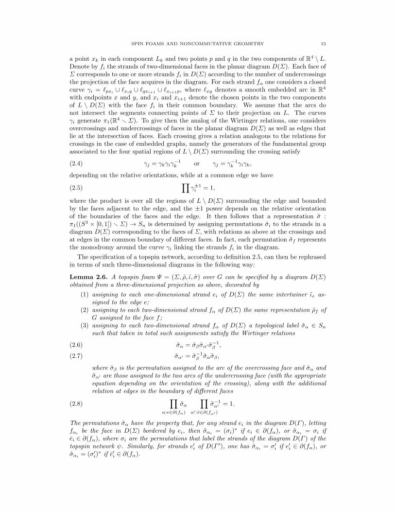
a point xk in each component Lk and two points p and q in the two components of R4 \ L.Denote by fi the strands of two-dimensional faces in the planar diagram D(Σ). Each face ofΣ corresponds to one or more strands fi in D(Σ) according to the number of undercrossingsthe projection of the face acquires in the diagram. For each strand fα one considers a closedcurve γi = `pxi ∪ `xiq ∪ `qxi+1
∪ `xi+1p, where `xy denotes a smooth embedded arc in R4
with endpoints x and y, and xi and xi+1 denote the chosen points in the two componentsof L \ D(Σ) with the face fi in their common boundary. We assume that the arcs donot intersect the segments connecting points of Σ to their projection on L. The curvesγi generate π1(R4 r Σ). To give then the analog of the Wirtinger relations, one considersovercrossings and undercrossings of faces in the planar diagram D(Σ) as well as edges thatlie at the intersection of faces. Each crossing gives a relation analogous to the relations forcrossings in the case of embedded graphs, namely the generators of the fundamental groupassociated to the four spatial regions of L \D(Σ) surrounding the crossing satisfy
(2.4) γj = γkγiγ−1k or γj = γ−1
k γiγk,
depending on the relative orientations, while at a common edge we have
(2.5)∏
γ±1i = 1,
where the product is over all the regions of L \ D(Σ) surrounding the edge and boundedby the faces adjacent to the edge, and the ±1 power depends on the relative orientationof the boundaries of the faces and the edge. It then follows that a representation σ :π1((S3 × [0, 1]) r Σ) → Sn is determined by assigning permutations σi to the strands in adiagram D(Σ) corresponding to the faces of Σ, with relations as above at the crossings andat edges in the common boundary of different faces. In fact, each permutation σf representsthe monodromy around the curve γi linking the strands fi in the diagram.
The specification of a topspin network, according to definition 2.5, can then be rephrasedin terms of such three-dimensional diagrams in the following way:
Lemma 2.6. A topspin foam Ψ = (Σ, ρ, ι, σ) over G can be specified by a diagram D(Σ)obtained from a three-dimensional projection as above, decorated by
(1) assigning to each one-dimensional strand ei of D(Σ) the same intertwiner ιe as-signed to the edge e;
(2) assigning to each two-dimensional strand fα of D(Σ) the same representation ρf ofG assigned to the face f ;
(3) assigning to each two-dimensional strand fα of D(Σ) a topological label σα ∈ Snsuch that taken in total such assignments satisfy the Wirtinger relations
σα = σβ σα′ σ−1β ,(2.6)
σα′ = σ−1β σασβ ,(2.7)
where σβ is the permutation assigned to the arc of the overcrossing face and σα andσα′ are those assigned to the two arcs of the undercrossing face (with the appropriateequation depending on the orientation of the crossing), along with the additionalrelation at edges in the boundary of different faces
(2.8)∏
α:e∈∂(fα)
σα∏
α′:e∈∂(fα′ )
σ−1α′ = 1.
The permutations σα have the property that, for any strand ei in the diagram D(Γ ), lettingfαi be the face in D(Σ) bordered by ei, then σαi = (σi)
∗ if ei ∈ ∂(fα), or σαi = σi ifei ∈ ∂(fα), where σi are the permutations that label the strands of the diagram D(Γ ) of thetopspin network ψ. Similarly, for strands e′i of D(Γ ′), one has σαi = σ′i if e′i ∈ ∂(fα), orσαi = (σ′i)
∗ if e′i ∈ ∂(fα).

16 DOMENIC DENICOLA, MATILDE MARCOLLI, AND AHMAD ZAINY AL-YASRY
Proof. We can consider Σ ⊂ S3 × [0, 1] as embedded in S4, with the four-sphere obtainedby cupping Σ ⊂ S3 × [0, 1] with two 3-balls D3 glued along the two boundary componentsS3 × {0} and S3 × {1}. By removing the point at infinity, we can then think of Σ asembedded in R4 and obtain diagrams D(Σ) by projections on generic three-dimensionallinear subspaces in R4, where one marks by overcrossings and undercrossings the strands ofΓ that intersect in the projection, as in the case of embedded knots and graphs.
We can then use the presentation of the fundamental group of the complement π1(S4rΣ)given in terms of generators and Wirtinger relations as above. This shows that the dataσα define a representation σ : π1(S4 r Σ) → Sn, hence an n-fold branched covering of S4
branched along Σ. The compatibility with σα and the σi and σ′i show that the restrictionof this branched covering to S3 × [0, 1] determines a branched cover cobordism betweenthe covering M and M ′ of the three-sphere, respectively determined by the representationsσ : π1(S3 r Γ ) → Sn and σ′ : π1(S3 r Γ ′) → Sn. We use here the fact that, near theboundary, the embedded two-complex Σ is a product Γ × [0, ε) or (−ε, 0]× Γ ′. �
2.8. The case of cyclic coverings. A cyclic branched covering M of S3, branched alongΓ ⊂ S3, is a branched covering such that the corresponding representation σ maps surjec-tively
(2.9) σ : π1(S3 r Γ )→ Z/nZ.Topspin networks whose topological data define cyclic branched coverings are simpler thanthe general case discussed above, in the sense that the topological data are directly associatedto the graph Γ itself, not to the planar projections D(Γ ).
Proposition 2.7. Let ψ = (Γ, ρ, ι, σ) be a topspin network such that the branched coverM of S3 determined by (Γ, σ) is cyclic. Then the data ψ = (Γ, ρ, ι, σ) are equivalent to aspin networks (Γ, ρ, ι) together with group elements σe ∈ Z/nZ associated to the edges of Γsatisfying the relation
(2.10)∏
s(ei)=v
σei∏
t(ej)=v
σ−1ej = 1.
Proof. In terms of the Wirtinger presentation of π1(S3 r Γ ) associated to the choice of aplanar diagram D(Γ ) of the graph Γ , we see that, because the range of the representationσ is the abelian group Z/nZ, the Wirtinger relations at crossings eqs. (2.1) and (2.2) simplygive σi = σj , which means that the group elements assigned to all the strands in the planardiagram D(Γ ) belonging to the same edge of Γ are equal. Equivalently, the topologicallabels just consist of group elements σe ∈ Z/nZ attached to the edges of Γ . The remainingWirtinger relation eq. (2.3) then gives eq. (2.10). �
For such cyclic coverings, we can also introduce a notion of degenerate topspin networks.One may regard them as analogous to the degenerate Q-lattices of [19] in our analogy witharithmetic noncommutative geometry discussed in section 4 below. However, while in theQ-lattices case it is crucial to include the non-invertible (degenerate) Q-lattices in order tohave a noncommutative space describing the quotient by commensurability and a dynam-ical flow on the resulting convolution algebra, in the setting we are considering here onealready obtains an interesting algebra and dynamics on it just by restricting to the ordinary(nondegenerate) topspin foams and networks. In fact, the equivalence relation determinedby stabilization and covering moves suffices to give rise to a system with properties similarto those of the Q-lattices case.
Definition 2.8. A possibly-degenerate topspin network over a compact Lie group G is atuple (Γ, ρ, ι, σ) of data consisting of
(1) a spin network (Γ, ρ, ι) in the sense of definition 2.1, with Γ ⊂ S3;(2) a labeling σ of each e of Γ by a cyclic permutation σe ∈ Z/nZ.
SPIN FOAMS AND NONCOMMUTATIVE GEOMETRY 17KHOVANOV HOMOLOGY AND EMBEDDED GRAPHS 3
Saddle Point
Saddle Point
After
Before
FIGURE 2. Saddle Point
there is only one saddle point between the two cross sections and if the number of components de-
creases. We can define analogously a positive hyperbolic transformation.
Definition 2.1. [6] We say that two knots K1 and K2 are related by an elementary cobordism if the
knot K2 is obtained by r! 1 negative hyperbolic transformations from a split link consisting of K1
together with r! 1 circles.
What we mean by split link is a link with n components (Ki, i = 1....n) in S3 such that there are
mutually disjoint n 3-cells (Di, i= 1....n) containing Ki, i= 1,2...,n
Lemma 2.2. [6] Two knots are called knot cobordic if and only if they are related by a sequence of
elementary cobordisms
It is well known that the oriented knots form a commutative semigroup under the operation of
composition #. Given two knots K1 and K2, we can obtain a new knot by removing a small arc from
each knot and then connecting the four endpoints by two new arcs. The resulting knot is called the
composition of the two knots K1 and K2 and is denoted by K1#K2.
Notice that, if we take the composition of a knot K with the unknot " then the result is again K.
Lemma 2.3. The set of oriented knots with the connecting operation # forms a semigroup with identity
"Fox and Milnor [2] showed that composition of knots induces a composition on knot cobordism
classes [K]#[K#]. This gives an abelian groupGK with ["] as identity and the negative is ![K] = [!K],where the !K denotes the reflected inverse of K.
Theorem 2.4. The knot cobordism classes with the connected sum operation # form an abelian group,
called the knot cobordism group and denoted by GK.
2.2. Link cobordism group. [6] For links, the conjunction operation & between two links gives a
commutative semigroup. L1&L2 is a link represented by the union of the two links l1 $ l2 where l1represents L1 and l2 represents L2 with mutually disjoint 3-cells D1 and D2 contain l1 and l2 respec-
tively. Here “represents” means that we are working with ambient isotopy classes Li of links (also
called link types) and the li are chosen representatives of these classes. In the following we loosely
refer to the classes Li also simply as links, with the ambient isotopy equivalence implicitly under-
stood. The zero of this semigroup is the link consisting of just the empty link. The link cobordism
group is constructed using the conjunction operation and the cobordism classes. We recall below the
definition of cobordism of links.
Let L be a link in S3 containing r-components k1, ....,kr with a split sublink Ls = k1 $k2 $ ....$kt , t % r
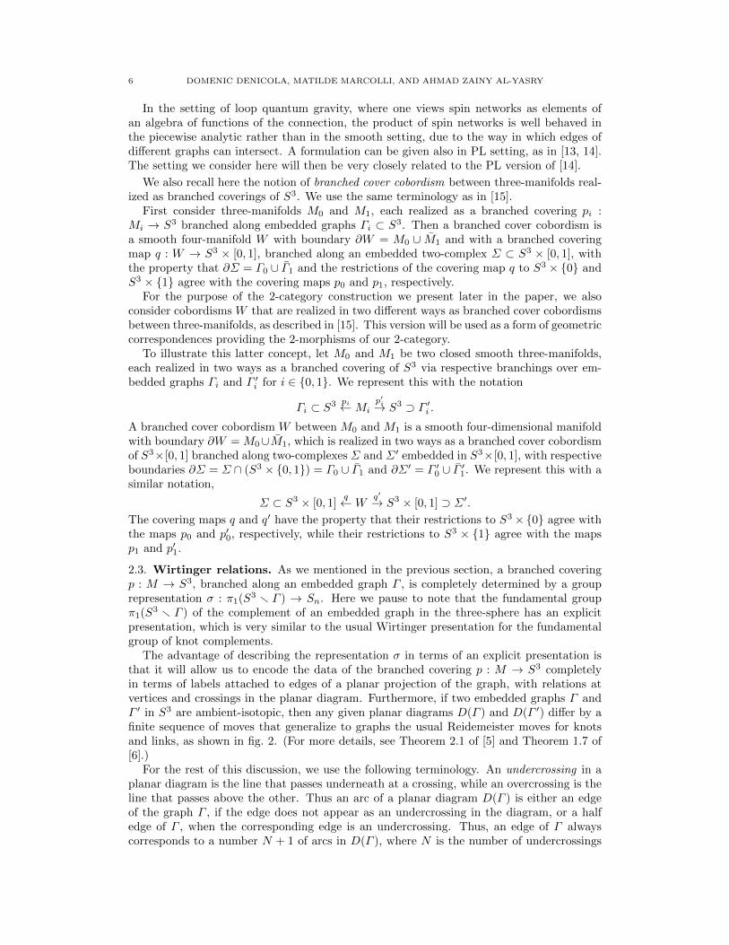
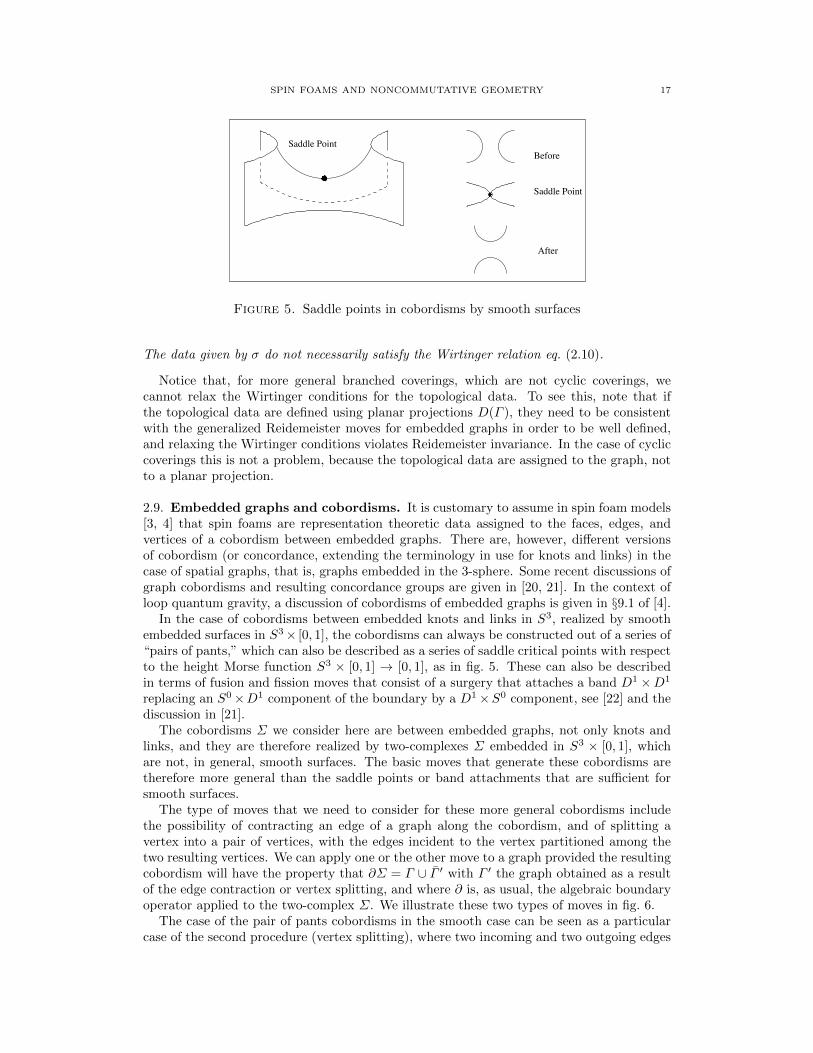
Figure 5. Saddle points in cobordisms by smooth surfaces
The data given by σ do not necessarily satisfy the Wirtinger relation eq. (2.10).
Notice that, for more general branched coverings, which are not cyclic coverings, wecannot relax the Wirtinger conditions for the topological data. To see this, note that ifthe topological data are defined using planar projections D(Γ ), they need to be consistentwith the generalized Reidemeister moves for embedded graphs in order to be well defined,and relaxing the Wirtinger conditions violates Reidemeister invariance. In the case of cycliccoverings this is not a problem, because the topological data are assigned to the graph, notto a planar projection.
2.9. Embedded graphs and cobordisms. It is customary to assume in spin foam models[3, 4] that spin foams are representation theoretic data assigned to the faces, edges, andvertices of a cobordism between embedded graphs. There are, however, different versionsof cobordism (or concordance, extending the terminology in use for knots and links) in thecase of spatial graphs, that is, graphs embedded in the 3-sphere. Some recent discussions ofgraph cobordisms and resulting concordance groups are given in [20, 21]. In the context ofloop quantum gravity, a discussion of cobordisms of embedded graphs is given in §9.1 of [4].
In the case of cobordisms between embedded knots and links in S3, realized by smoothembedded surfaces in S3× [0, 1], the cobordisms can always be constructed out of a series of“pairs of pants,” which can also be described as a series of saddle critical points with respectto the height Morse function S3 × [0, 1] → [0, 1], as in fig. 5. These can also be describedin terms of fusion and fission moves that consist of a surgery that attaches a band D1 ×D1
replacing an S0×D1 component of the boundary by a D1×S0 component, see [22] and thediscussion in [21].
The cobordisms Σ we consider here are between embedded graphs, not only knots andlinks, and they are therefore realized by two-complexes Σ embedded in S3 × [0, 1], whichare not, in general, smooth surfaces. The basic moves that generate these cobordisms aretherefore more general than the saddle points or band attachments that are sufficient forsmooth surfaces.
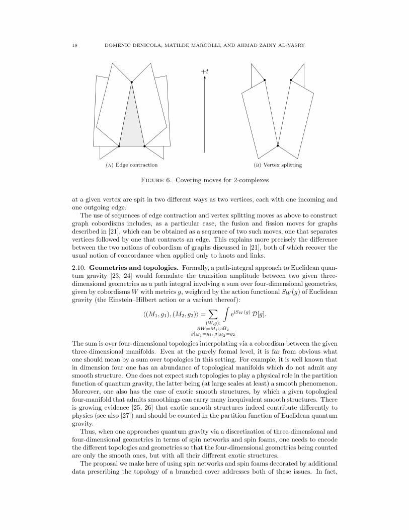
The type of moves that we need to consider for these more general cobordisms includethe possibility of contracting an edge of a graph along the cobordism, and of splitting avertex into a pair of vertices, with the edges incident to the vertex partitioned among thetwo resulting vertices. We can apply one or the other move to a graph provided the resultingcobordism will have the property that ∂Σ = Γ ∪ Γ ′ with Γ ′ the graph obtained as a resultof the edge contraction or vertex splitting, and where ∂ is, as usual, the algebraic boundaryoperator applied to the two-complex Σ. We illustrate these two types of moves in fig. 6.
The case of the pair of pants cobordisms in the smooth case can be seen as a particularcase of the second procedure (vertex splitting), where two incoming and two outgoing edges
18 DOMENIC DENICOLA, MATILDE MARCOLLI, AND AHMAD ZAINY AL-YASRY
(a) Edge contraction
+t
6
(b) Vertex splitting
Figure 6. Covering moves for 2-complexes
at a given vertex are spit in two different ways as two vertices, each with one incoming andone outgoing edge.
The use of sequences of edge contraction and vertex splitting moves as above to constructgraph cobordisms includes, as a particular case, the fusion and fission moves for graphsdescribed in [21], which can be obtained as a sequence of two such moves, one that separatesvertices followed by one that contracts an edge. This explains more precisely the differencebetween the two notions of cobordism of graphs discussed in [21], both of which recover theusual notion of concordance when applied only to knots and links.
2.10. Geometries and topologies. Formally, a path-integral approach to Euclidean quan-tum gravity [23, 24] would formulate the transition amplitude between two given three-dimensional geometries as a path integral involving a sum over four-dimensional geometries,given by cobordisms W with metrics g, weighted by the action functional SW (g) of Euclideangravity (the Einstein–Hilbert action or a variant thereof):
〈(M1, g1), (M2, g2)〉 =∑
(W,g):∂W=M1∪M2
g|M1=g1, g|M2
=g2
∫eiSW (g)D[g].
The sum is over four-dimensional topologies interpolating via a cobordism between the giventhree-dimensional manifolds. Even at the purely formal level, it is far from obvious whatone should mean by a sum over topologies in this setting. For example, it is well known thatin dimension four one has an abundance of topological manifolds which do not admit anysmooth structure. One does not expect such topologies to play a physical role in the partitionfunction of quantum gravity, the latter being (at large scales at least) a smooth phenomenon.Moreover, one also has the case of exotic smooth structures, by which a given topologicalfour-manifold that admits smoothings can carry many inequivalent smooth structures. Thereis growing evidence [25, 26] that exotic smooth structures indeed contribute differently tophysics (see also [27]) and should be counted in the partition function of Euclidean quantumgravity.
Thus, when one approaches quantum gravity via a discretization of three-dimensional andfour-dimensional geometries in terms of spin networks and spin foams, one needs to encodethe different topologies and geometries so that the four-dimensional geometries being countedare only the smooth ones, but with all their different exotic structures.
The proposal we make here of using spin networks and spin foams decorated by additionaldata prescribing the topology of a branched cover addresses both of these issues. In fact,
SPIN FOAMS AND NONCOMMUTATIVE GEOMETRY 19
the main result we refer to in the case of four-dimensional geometries, is the description ofall compact PL four-manifolds as branched coverings of the four-sphere, obtained in [12].Since in the case of four-manifolds one can upgrade PL structures to smooth structures, thisalready selects only those four-manifolds that admit a smooth structures, and moreover itaccounts for the different exotic structures.
3. Noncommutative spaces as algebras and categories
Noncommutative spaces are often described either as algebras or as categories. In fact,there are several instances in which one can convert the data of a (small) category into analgebra and conversely.
3.1. Algebras from categories. We recall here briefly some well known examples in non-commutative geometry which can be described easily in terms of associative algebras deter-mined by categories. We then describe a generalization to the case of 2-categories.
Example 3.1. The first example, and prototype for the generalizations that follow, isthe well known construction of the (reduced) group C∗-algebra. Suppose we are given adiscrete group G. Let C[G] be the group ring. Elements in C[G] can be described as finitelysupported functions f : G→ C, with the product given by the convolution product
(f1 ? f2)(g) =∑
g=g1g2
f1(g1)f2(g2).
This product is associative but not commutative. The involution f∗(g) ≡ f(g−1) satisfies(f1?f2)∗ = f∗2 ?f
∗1 and makes the group ring into an involutive algebra. The norm closure in
the representation π : C[G] → B(`2(G)), given by (π(f)ξ)(g) =∑g=g1g2
f(g1)ξ(g2), defines
the reduced group C∗-algebra C∗r (G).
Example 3.2. The second example is similar, but one considers a discrete semigroup Sinstead of a group G. One can still form the semigroup ring C[S] given by finitely supportedfunctions f : S → C with the convolution product
(f1 ? f2)(s) =∑
s=s1s2
f1(s1)f2(s2).
Since this time elements of S do not, in general, have inverses, one no longer has theinvolution as in the group ring case. One can still represent C[S] as bounded operators actingon the Hilbert space `2(S), via (π(f)ξ)(s) =
∑s=s1s2
f(s1)ξ(s2) This time the elements s ∈ Sact on `2(S) by isometries, instead of unitary operators as in the group case. In fact, thedelta function δs acts on the basis element εs′ as a multiplicative shift, δs : εs′ 7→ εss′ . If onedenotes by π(f)∗ the adjoint of π(f) as an operator on the Hilbert space `2(S), then onehas δ∗sδs = 1 but δsδ
∗s = es is an idempotent not equal to the identity. One can consider
then the C∗-algebra C∗r (S), which is the C∗-subalgebra of B(`2(S)) generated by the δs andtheir adjoints.
Example 3.3. The third example is the groupoid case: a groupoid G = (G(0),G(1), s, t) is a(small) category with a collection of objects G(0) also called the units of the groupoids, andwith morphisms γ ∈ G(1), such that all morphisms are invertible. There are source and targetmaps s(γ), t(γ) ∈ G(0), so that, with the equivalent notation used above γ ∈ MorG(s(γ), t(γ)).One can view G(0) ⊂ G(1) by identifying x ∈ G(0) with the identity morphisms 1x ∈ G(1).The composition γ1 ◦ γ2 of two elements γ1 and γ2 in G(1) is defined under the conditionthat t(γ2) = s(γ1). Again we assume here for simplicity that G(0) and G(1) are sets with thediscrete topology. One considers then a groupoid ring C[G] of finitely supported functionsf : G(1) → C with convolution product
(f1 ? f2)(γ) =∑
γ=γ1◦γ2
f1(γ1)f2(γ2).
20 DOMENIC DENICOLA, MATILDE MARCOLLI, AND AHMAD ZAINY AL-YASRY
Since a groupoid is a small category where all morphisms are invertible, there is an involutionon C[G] given again, as in the group case, by f∗(γ) = f(γ−1). In fact, the group case is aspecial case where the category has a single object. One obtains C∗-norms by considering
representations πx : C[G] → B(`2(G(1)x )), where G(1)
x = {γ ∈ G(1) : s(γ) = x}, given by(πx(f)ξ)(γ) =
∑γ=γ1◦γ2 f(γ1)ξ(γ2). This is well defined since for the composition s(γ) =
s(γ2). One has corresponding norms ‖f‖x = ‖πx(f)‖B(`2(G(1)x ))
and C∗-algebra completions.
Example 3.4. The generalization of both the semigroup and the groupoid case is then thecase of a semigroupoid, which is the same as a small category S. In this case one can describethe data Obj(S) and MorS(x, y) for x, y ∈ Obj(S) in terms of S = (S(0),S(1), s, t) as in thegroupoid case, but without assuming the invertibility of morphisms. The the algebra C[S]of finitely supported functions on S(1) with convolution product
(f1 ? f2)(φ) =∑
φ=φ1◦φ2
f1(φ1)f2(φ2)
is still defined as in the groupoid case, but without the involution. One still has representa-
tions πx : C[G]→ B(`2(S(1)x )) as in the groupoid case.
Example 3.5. A simple example of C∗-algebras associated to small categories is given bythe graph C∗-algebras. Consider for simplicity a finite oriented graph Γ . It can be thoughtof as a small category with objects the vertices v ∈ V (Γ ) and morphisms the oriented edgese ∈ E(Γ ). The source and target maps are given by the boundary vertices of edges. Thesemigroupoid algebra is then generated by a partial isometry δe for each oriented edge withsource projections ps(e) = δ∗eδe. One has the relation pv =
∑s(e)=v δeδ
∗e .
Example 3.6. The convolution algebra associated to a small category S is constructedin such a way that the product follows the way morphisms can be decomposed in thecategory as a composition of two other morphisms. When one has a category with sufficientextra structure, one can do a similar construction of an associative algebra based on adecomposition of objects instead of morphisms. This is possible when one has an abeliancategory C, and one associates to it a Ringel–Hall algebra, see [28]. One considers the setIso(C) of isomorphism classes of objects and functions with finite support f : Iso(C) → Cwith the convolution product
(f1 ? f2)(X) =∑X′⊂X
f1(X ′)f2(X/X ′),
with the splitting of the object X corresponding to the exact sequence
0→ X ′ → X → X/X ′ → 0.
All these instances of translations between algebras and categories can be interpretedwithin the general framework of “categorification” phenomena. We will not enter here intodetails on any of these examples. We give instead an analogous construction of a convolutionalgebra associated to a 2-category. This type of algebras were used both in [15] and in [29];here we give a more detailed discussion of their properties.
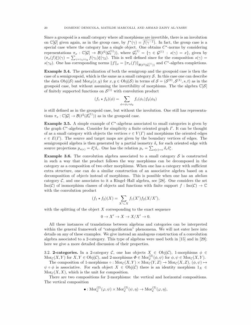
3.2. 2-categories. In a 2-category C, one has objects X ∈ Obj(C), 1-morphisms φ ∈MorC(X,Y ) for X,Y ∈ Obj(C), and 2-morphisms Φ ∈ Mor
(2)C (φ, ψ) for φ, ψ ∈ MorC(X,Y ).
The composition of 1-morphisms ◦ : MorC(X,Y )×MorC(Y, Z)→ MorC(X,Z), (φ, ψ) 7→ψ ◦ φ is associative. For each object X ∈ Obj(C) there is an identity morphism 1X ∈MorC(X,X), which is the unit for composition.
There are two compositions for 2-morphisms: the vertical and horizontal compositions.The vertical composition
• : Mor(2)C (ϕ,ψ)×Mor
(2)C (ψ, η)→ Mor
(2)C (ϕ, η),
SPIN FOAMS AND NONCOMMUTATIVE GEOMETRY 21
which is defined for ϕ,ψ, η ∈ MorC(X,Y ), is associative and has identity elements 1φ ∈Mor
(2)C (φ, φ).
The horizontal composition
◦ : Mor(2)C (ϕ,ψ)×Mor
(2)C (ξ, η)→ Mor
(2)C (ξ ◦ ϕ, η ◦ ψ),
which follows the composition of 1-morphisms and is therefore defined for ϕ,ψ ∈ MorC(X,Y )and ξ, η ∈ MorC(Y, Z), is also required to be associative. It also has a unit element, givenby the identity 2-morphism between the identity morphisms IX ∈ Mor
(2)C (1X , 1X).
The compatibility between vertical and horizontal composition is given by
(3.1) (Φ1 ◦ Ψ1) • (Φ2 ◦ Ψ2) = (Φ1 • Φ2) ◦ (Ψ1 • Ψ2).
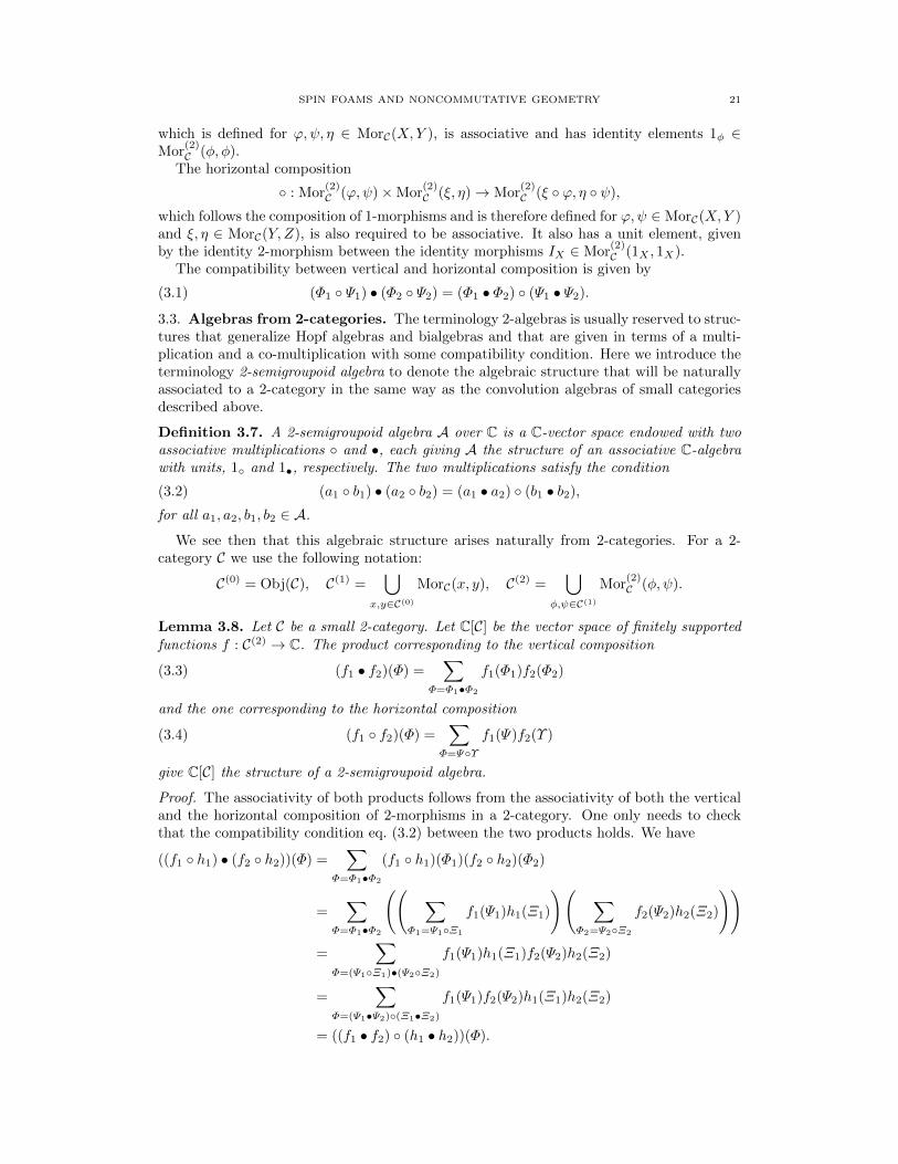
3.3. Algebras from 2-categories. The terminology 2-algebras is usually reserved to struc-tures that generalize Hopf algebras and bialgebras and that are given in terms of a multi-plication and a co-multiplication with some compatibility condition. Here we introduce theterminology 2-semigroupoid algebra to denote the algebraic structure that will be naturallyassociated to a 2-category in the same way as the convolution algebras of small categoriesdescribed above.
Definition 3.7. A 2-semigroupoid algebra A over C is a C-vector space endowed with twoassociative multiplications ◦ and •, each giving A the structure of an associative C-algebrawith units, 1◦ and 1•, respectively. The two multiplications satisfy the condition
(3.2) (a1 ◦ b1) • (a2 ◦ b2) = (a1 • a2) ◦ (b1 • b2),
for all a1, a2, b1, b2 ∈ A.
We see then that this algebraic structure arises naturally from 2-categories. For a 2-category C we use the following notation:
C(0) = Obj(C), C(1) =⋃
x,y∈C(0)MorC(x, y), C(2) =
⋃φ,ψ∈C(1)
Mor(2)C (φ, ψ).
Lemma 3.8. Let C be a small 2-category. Let C[C] be the vector space of finitely supportedfunctions f : C(2) → C. The product corresponding to the vertical composition
(3.3) (f1 • f2)(Φ) =∑
Φ=Φ1•Φ2
f1(Φ1)f2(Φ2)
and the one corresponding to the horizontal composition
(3.4) (f1 ◦ f2)(Φ) =∑
Φ=Ψ◦Υf1(Ψ)f2(Υ )
give C[C] the structure of a 2-semigroupoid algebra.
Proof. The associativity of both products follows from the associativity of both the verticaland the horizontal composition of 2-morphisms in a 2-category. One only needs to checkthat the compatibility condition eq. (3.2) between the two products holds. We have
((f1 ◦ h1) • (f2 ◦ h2))(Φ) =∑
Φ=Φ1•Φ2
(f1 ◦ h1)(Φ1)(f2 ◦ h2)(Φ2)
=∑
Φ=Φ1•Φ2
(( ∑Φ1=Ψ1◦Ξ1
f1(Ψ1)h1(Ξ1)
)( ∑Φ2=Ψ2◦Ξ2
f2(Ψ2)h2(Ξ2)
))=
∑Φ=(Ψ1◦Ξ1)•(Ψ2◦Ξ2)
f1(Ψ1)h1(Ξ1)f2(Ψ2)h2(Ξ2)
=∑
Φ=(Ψ1•Ψ2)◦(Ξ1•Ξ2)
f1(Ψ1)f2(Ψ2)h1(Ξ1)h2(Ξ2)
= ((f1 • f2) ◦ (h1 • h2))(Φ).
22 DOMENIC DENICOLA, MATILDE MARCOLLI, AND AHMAD ZAINY AL-YASRY
�
A 2-semigroupoid algebra corresponding to a 2-category of low dimensional geometrieswas considered in [15], as the “algebra of coordinates” of a noncommutative space of geome-tries. A similar construction of a 2-semigroupoid algebra coming from surgery presentationsof three-manifolds was considered in [29].
4. A model case from arithmetic noncommutative geometry
We discuss here briefly a motivating construction that arises in another context in non-commutative geometry, in applications of the quantum statistical mechanical formalism toarithmetic of abelian extensions of number fields and function fields. We refer the reader toChapter 3 of the book [19] for a detailed treatment of this topic.
The main feature of the construction we review below, which is directly relevant to our set-ting of spin networks and spin foams, is the following. One considers a space parameterizinga certain family of possibly singular geometries. In the arithmetic setting these geometriesare pairs of an n-dimensional lattice Λ and a group homomorphism φ : Qn/Zn → QΛ/Λ,which can be thought of as a (possibly degenerate) level structure, a labeling of the torsionpoints of the lattice Λ in terms of the torsion points of the “standard lattice.” Among thesegeometries one has the “nonsingular ones,” which are those for which the labeling φ is anactual level structure, that is, a group isomorphism. On this set of geometries there is anatural equivalence relation, which is given by commensurability of the lattices, QΛ1 = QΛ2
and identification of the labeling functions, φ1 = φ2 modulo Λ1 + Λ2. One forms a convo-lution algebra associated to this equivalence relation, which gives a noncommutative spaceparameterizing the moduli space of these geometries up to commensurability.
The resulting convolution algebra has a natural time evolution, which can be describedin terms of the covolume of lattices. The resulting quantum statistical mechanical systemexhibits a spontaneous symmetry breaking phenomenon. Below the critical temperature,the extremal low temperature KMS equilibrium states of the system automatically selectonly those geometries that are nondegenerate.
This provides a mechanism by which the correct type of geometries spontaneously emergeas low temperature equilibrium states. A discussion of this point of view on emergentgeometry can be found in §8 of Chapter 4 of [19].
The reason why this is relevant to the setting of spin foam models is that one can similarlyconsider a convolution algebra that parameterizes all (possibly degenerate) topspin foamscarrying the metric and topological information on the quantized four-dimensional geometry.One then looks for a time evolution on this algebra whose low temperature equilibrium stateswould automatically select, in a spontaneous symmetry breaking phenomenon, the correctnondegenerate geometries.
We recall in this section the arithmetic case, stressing the explicit analogies with the caseof spin foams we are considering here.
4.1. Quantum statistical mechanics. The formalism of Quantum Statistical Mechanicsin the operator algebra setting can be summarized briefly as follows. (See [30, 31] and §3 of[19] for a more detailed treatment.)
One has a (unital) C∗-algebra A of observables, together with a time evolution—that is,a one-parameter family of automorphisms σ : R→ Aut(A).
A state on the algebra of observables is a linear functional ϕ : A → C, which is normalizedby ϕ(1) = 1 and satisfies the positivity condition ϕ(a∗a) ≥ 0 for all a ∈ A.
Among states on the algebra, one looks in particular for those that are equilibrium statesfor the time evolution. This property is expressed by the KMS condition, which dependson a thermodynamic parameter β (the inverse temperature). Namely, a state ϕ is a KMSβstate for the dynamical system (A, σ) if for every choice of two elements a, b ∈ A there existsa function Fa,b(z) which is holomorphic on the strip in the complex plane Iβ = {z ∈ C :
SPIN FOAMS AND NONCOMMUTATIVE GEOMETRY 23
0 < =(z) < β} and extends to a continuous function to the boundary ∂Iβ of the strip, withthe property that, for all t ∈ R,
Fa,b(t) = ϕ(aσt(b)),
Fa,b(t+ iβ) = ϕ(σt(b)a).
This condition can be regarded as identifying a class of functionals which fail to be traces byan amount that is controlled by interpolation via a holomorphic function that analyticallycontinues the time evolution. An equivalent formulation of the KMS condition in fact statesthat the functional ϕ satisfies
ϕ(ab) = ϕ(bσiβ(a)),
for all a, b in a dense subalgebra of “analytic elements”.At zero temperature T ≡ 1/β = 0, the KMS∞ states are defined in [32] as the weak limits
of KMSβ states ϕ∞(a) = limβ→∞ ϕβ(a).KMS states are equilibrium states, namely one has ϕ(σt(a)) = ϕ(a) for all t ∈ R. This
can be seen from an equivalent formulation of the KMS condition as the identity ϕ(ab) =ϕ(bσiβ(a)) for all a, b in a dense subalgebra of analytic elements on which the time evolutionσt admits an analytic continuation σz, see [31] §5.
Given a representation π : A → B(H) of the algebra of observables as bounded operatorson a Hilbert space, one has a Hamiltonian H generating the time evolution σt if there is anoperator H (generally unbounded) on H satisfying
π(σt(a)) = eitHπ(a)e−itH
for all a ∈ A and for all t ∈ R.A particular case of KMS states is given by the Gibbs states
(4.1)1
Z(β)Tr(π(a) e−βH
),
with partition function Z(β) = Tr(e−βH
). However, while the Gibbs states are only defined
under the condition that the operator exp(−βH) is trace class, the KMS condition holdsmore generally and includes equilibrium states that are not of the Gibbs form.
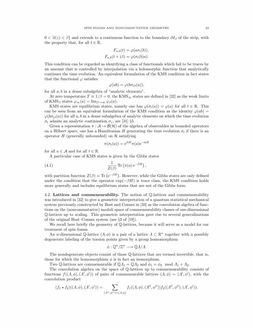
4.2. Lattices and commensurability. The notion of Q-lattices and commensurabilitywas introduced in [32] to give a geometric interpretation of a quantum statistical mechanicalsystem previously constructed by Bost and Connes in [33] as the convolution algebra of func-tions on the (noncommutative) moduli space of commensurability classes of one-dimensionalQ-lattices up to scaling. This geometric interpretation gave rise to several generalizationsof the original Bost–Connes system (see §3 of [19]).
We recall here briefly the geometry of Q-lattices, because it will serve as a model for ourtreatment of spin foams.
An n-dimensional Q-lattice (Λ, φ) is a pair of a lattice Λ ⊂ Rn together with a possiblydegenerate labeling of the torsion points given by a group homomorphism
φ : Qn/Zn −→ QΛ/Λ.
The nondegenerate objects consist of those Q-lattices that are termed invertible, that is,those for which the homomorphism φ is in fact an isomorphism.
Two Q-lattices are commensurable if QΛ1 = QΛ2 and φ1 = φ2 mod Λ1 + Λ2.The convolution algebra on the space of Q-lattices up to commensurability consists of
functions f((Λ, φ), (Λ′, φ′)) of pairs of commensurable lattices (Λ, φ) ∼ (Λ′, φ′), with theconvolution product
(f1 ? f2)((Λ, φ), (Λ′, φ′)) =∑
(Λ′′,φ′′)∼(Λ,φ)
f1((Λ, φ), (Λ′′, φ′′))f2((Λ′′, φ′′), (Λ′, φ′)).

24 DOMENIC DENICOLA, MATILDE MARCOLLI, AND AHMAD ZAINY AL-YASRY
In the case of one-dimensional or two-dimensional Q-lattices considered in [32], one cansimilarly consider the convolution algebra for the commensurability relation on Q-latticesconsidered up to a scaling action of R∗+ or C∗, respectively. One then has on the resultingalgebra a natural time evolution by the ratio of the covolumes of the pair of commensurablelattices,
σt(f)((Λ, φ), (Λ′, φ′)) =
(Vol(Rn/Λ′)Vol(Rn/Λ)
)it
f((Λ, φ), (Λ′, φ′)).
4.3. Low temperature KMS states. The quantum statistical mechanical systems of one-dimensional or two-dimensional Q-lattices introduced in [32] exhibit a pattern of symmetrybreaking and the low temperature extremal KMS states are parameterized by exactly thoseQ-lattices that give the nondegenerate geometries, the invertible Q-lattices.
One considers representations of the convolution algebra on the Hilbert space `2(C(Λ,φ)),with C(Λ,φ) the commensurability class of a given Q-lattice,
π(f)ξ(Λ′, φ′) =∑
(Λ′′,φ′′)∼(Λ,φ)
f((Λ′, φ′), (Λ′′, φ′′))ξ(Λ′′, φ′′).
In the case when (Λ, φ) is invertible, the Hamiltonian generating the time evolution in thisrepresentation has positive energy and one has a corresponding Gibbs KMS state
(4.2) ϕL,β(f) = Z(β)−1∑
m∈SL2(Z)\M+2 (Z)
f(mρ,m(z)) det(m)−β ,
for L = (Λ, φ) an invertible Q-lattice, where we use the parametrization as in [32] of the
invertible Q-lattice L = (Λ, φ) by a pair (ρ, z) of an element ρ ∈ GL2(Z) and a pointz ∈ H, and the Q-lattices in the commensurability class with elements (mρ,m(z)) withm ∈ SL2(Z)\M+
2 (Z). The partition function is Z(β) =∑
det(m)−β = ζ(β)ζ(β − 1). Acomplete characterization of extremal KMS states in terms of measures on the space ofinvertible Q-lattices was given in [32].
4.4. The paradigm of emergent geometry. Without entering into further details, theimportant observation here is the fact that the nondegenerate geometries (the invertibleQ-lattices) are selected out of a larger space containing all possibly degenerate geometries(all Q-lattices) via a dynamical phenomenon of spontaneous symmetry breaking.
This was discussed in §8 of Chapter 4 of [19], in order to propose a scenario of emergentgeometry according to which spacetime geometry should arise spontaneously as a symmetrybreaking phenomenon. The analogy described there is between the setting of Q-latticesrecalled here above and the setting of almost-commutative geometries used in the particlephysics models based on noncommutative geometry (see [34] and Chapter 1 of [19], as well assection 8 below). The proposed analog of the possibly degenerate Q-lattices is a degenerateversion of the notion of spectral triple in noncommutative geometry, regarded as a kind ofcorrespondence, while the nondegenerate geometries that provide physical models of matterand gravity are expected to arise dynamically through a symmetry breaking phenomenonas the invertible Q-lattices do. We present here a similar picture, where the analogy is nowbetween the case of Q-lattices and that of spin foam models.
In the setting we describe here, we obtain a noncommutative space by considering topspinfoams and networks (our analog of Q-lattices) with the equivalence relation generated bycovering moves, which plays the role of commensurability, and the dynamics is generated bythe lack of invariance under these moves of the spin foam amplitudes. Other more elaborateconstructions based on composition operations of topspin foams, which we describe in thefollowing sections, also fit into a similar conceptual picture.
A frequent problem with the construction of spin foam models through combinatorialdata of simplicial complexes with spin labels is that one often obtains, along with ordinarysmooth geometries, also spurious solutions that do not correspond to manifolds and which are
SPIN FOAMS AND NONCOMMUTATIVE GEOMETRY 25
often difficult to recognize and separate from the “good solutions.” The idea of spontaneousemergence of geometry as a symmetry breaking phenomenon proposed in [19] suggests thatthe correct solutions, or nondegenerate geometries, should arise as low temperature extremalKMS equilibrium states from a natural dynamics on a noncommutative space describing theoverall moduli space of all possibly-degenerate geometries. Thus, the type of convolutionalgebras with dynamics that we consider here may also have possible generalizations thataddress this problem.
5. Categories of topspin networks and foams
We give here two natural constructions of categories of topspin networks and foams andthe corresponding algebras. These will serve as a simpler toy model, before we discuss themore elaborate construction of the 2-category in section 6 below.
5.1. The groupoid of topspin networks and covering moves. Let G denote thegroupoid of the equivalence relation on topspin networks generated by stabilization andcovering moves. The objects of G are topspin networks ψ = (Γ, ρ, ι, σ) and the morphismsare pairs (ψ,ψ′) of topspin foams such that the data (Γ, σ) and (Γ ′, σ′) are related, afterstabilization, by a finite sequence of covering moves. The data (ρ, ι) and (ρ′, ι′) are relatedby the compatibility conditions of section 2.6.
We consider then the groupoid algebra C[G] of finitely supported functions f(ψ,ψ′) ofpairs of covering moves equivalent topspin networks, with the convolution product
f1 ? f2(ψ,ψ′) =∑
ψ∼ψ′′∼ψ′f1(ψ,ψ′′)f2(ψ′′, ψ′).
One can construct a similar groupoid using topspin foams Ψ = (Σ, ρ, ι, σ) and the sameequivalence relation Ψ ∼ Ψ ′ when (Σ, σ) and (Σ′, σ′) determine the same four-manifold,expressed in terms of stabilizations and covering moves in the four-dimensional setting. Thecorresponding groupoid algebra of functions f(Ψ) has convolution product as above
f1 ? f2(Ψ, Ψ ′) =∑
Ψ∼Ψ ′′∼Ψ ′f1(Ψ, Ψ ′′)f2(Ψ ′′, Ψ ′).
5.2. The category of topspin networks and foams. We can also consider the usualcategory of spin networks and foams used in loop quantum gravity, which has objects thatare spin networks and morphisms that are spin foams cobordisms. One can enrich it withtopological data and obtain a category, or semigroupoid, S whose objects are topspin net-works ψ = (Γ, ρ, ι, σ) and whose morphisms MorC(ψ,ψ
′) are topspin foams Ψ = (Σ, ρ, ι, σ)cobordisms with ∂Σ = Γ ∪ Γ ′ and compatible data (ρ, ι, σ).
Again, one can associate to this category the semigroupoid algebra C[S] of functions offinite support f(Ψ) with convolution product
f1 ? f2(Ψ) =∑
Ψ=Ψ1Ψ2
f1(Ψ1)f2(Ψ2),
where the composition of topspin foams is obtained by gluing them along a common bound-ary topspin network.
5.3. Including degenerate geometries. A variant of the categories G and S describedabove can be obtained by restricting to cyclic coverings. In that case, we can include amongthe objects also the degenerate topspin networks and topspin foams, as in definition 2.8.The covering moves would still be the same, and the topspin cobordisms would also be asbefore, except that among the cobordisms one also allows for those where the Wirtingerrelations at edges for the data σf is not imposed. This variants allows us to illustrate, inthis toy model, a simple dynamical mechanisms that selects the nondegenerate geometriesamong the degenerate ones.
26 DOMENIC DENICOLA, MATILDE MARCOLLI, AND AHMAD ZAINY AL-YASRY
5.4. Representations. We consider the usual representations of C[G] on the Hilbert space
spanned by the arrows in the groupoid with fixed source, `2(G′(1)ψ ). This is the space `2(Cψ′)
of the equivalence class Cψ′ = {ψ : ψ ∼ ψ′} under the equivalence relation determined bystabilizations and covering moves. The representation πψ′ of C[G] on this Hilbert space isthen given by
πψ′(f)ξ(ψ) =∑
ψ′′∼ψ∼ψ′f(ψ,ψ′′)ξ(ψ′′),
where we have identified, in the standard way, an element ξ ∈ `2(Cψ′) with a square integrablefunction ξ on the set of ψ ∈ Cψ′ .
The case of the groupoid of the covering moves equivalence on topspin foams is analogous,with
πΨ ′(f)ξ(Ψ) =∑
Ψ ′′∼Ψ∼Ψ ′f(Ψ, Ψ ′′)ξ(Ψ ′′).
In a similar way, in the case of C[S] we can consider representations on a Hilbert spaceHψ,which in this case is spanned by all the topspin foams Ψ with ψ ⊂ ∂Ψ . The representationis again given by the same convolution product
πψ(f)ξ(Ψ) =∑
Ψ=Ψ1Ψ2 :ψ⊂∂Ψ2
f(Ψ1)ξ(Ψ2).
5.5. Dynamics on algebras of topspin networks and foams. In general spin foammodels [3, 4], one assigns to a spin foam Ψ = (Σ, ρ, ι) an amplitude of the form
(5.1) A(Ψ) = ω(Σ)∏f
Af (ρf )∏e
Ae(ρF (e), ιe)∏v
Av(ρF (v), ιE(v)),
where the weight factor ω(Σ) is a term that depends only on the two-complex Σ, whilethe amplitude Af at a given face depends on the representation ρf , the amplitude Ae ata given edge depends on the representations ρF (e) assigned to the faces adjacent to thatedge and on the intertwiner ιe at the edge, and the amplitude Av at a vertex depends onthe representations ρF (v) and intertwiners ιE(v) of the faces and edges adjacent to the givenvertex. One obtains the transition amplitudes between spin networks ψ and ψ′ by summingall the A(Ψ) for all the spin foams connecting ψ and ψ′.
We introduced topspin networks and topspin foams as a way to encode the topology ofthe underlying manifold as part of the discrete combinatorial data of quantized geometry.Thus, topspin networks and topspin foams that are related by covering moves, with thecorrect compatibility conditions on the representation theoretic data, should be regarded asdescribing the same quantum geometry. However, it is not always true that the spin foamamplitudes are necessarily invariant under covering moves. In a spin foam model where theamplitudes are not covering-moves invariant, this lack of invariance determines a nontrivialdynamics on the algebra of the groupoid of the equivalence relation.
For a choice of the amplitude (5.1) which is not invariant under covering moves, and forwhich the amplitudes are positive real numbers, one can define a dynamics on the groupoidalgebra of section 5.1 by setting
(5.2) σt(f)(Ψ, Ψ ′) =
(A(Ψ)
A(Ψ ′)
)it
f(Ψ, Ψ ′).
It is easy to check that this indeed defines a time evolution on the resulting groupoid algebra.Moreover, if one includes in the groupoid, in the case of topological data σ with values
in a cyclic group Z/nZ, also the degenerate topspin foams of definition 2.8, then one caninclude in the time evolution of eq. (5.2) a factor that measures how degenerate the geometryis.
SPIN FOAMS AND NONCOMMUTATIVE GEOMETRY 27
Let χ : S∞ → U(1) be a multiplicative character of the infinite symmetric group S∞ =⋃n Sn. We define an element W(ψ) ∈ Sn as the elements in the permutation group given
by the product of the Wirtinger relations at vertices:
W(ψ) ≡
∏v∈V (Γ )
∏e:v∈∂(e)
σe∏
e:v∈∂(e)
σ−1e
.
In fact, for cyclic coverings the elements W(Ψ) are contained in the subgroup Z/nZ of cyclicpermutations in Sn, so it suffices to take a character χ of U(1) and identify the elementsW(Ψ) with roots of unity in U(1).
This element is always W(ψ) = 1 for the nondegenerate geometries, while it can beW(ψ) 6= 1 in the degenerate cases. We can similarly define W(Ψ) for a degenerate topspinfoams, using the Wirtinger relation for faces incident to an edge,
(5.3) W(Ψ) ≡∏
f :e∈∂(f)
σf∏
f :e∈∂(f)
σ−1f .
With these in hand, we modify the time evolution of eq. (5.2) by setting
(5.4) σt(f)(Ψ, Ψ ′) =
(A(Ψ)
A(Ψ ′)
)it
χ(W(Ψ)W(Ψ ′)−1)t f(Ψ, Ψ ′).
In this way, the time evolution of eq. (5.4) accounts not only for the normalized amplitudediscrepancy between topspin foams related by covering moves, but also for the degeneracy ofthe geometry, measured by the failure if the topological data to satisfy the Wirtinger relationsand therefore define a genuine three-dimensional topology or four-dimensional cobordism.It is possible that more sophisticated examples of this type of dynamics may be constructedusing, instead of multiplicative characters of the infinite symmetric group, categorical rep-resentations of embedded graphs in the sense of [6] and quantum groups.
One can treat in a similar way the case of the algebra C[S] of topspin foams described insection 5.2. We define a normalized amplitude of the form
(5.5) A0(Ψ) =A(Ψ)
A(ψ0),
where Ψ is a spin foams connecting spin networks ψ0 and ψ1, with ∂Σ = Γ0 ∪ Γ1, and theamplitude for the spin network ψ0 is defined as
(5.6) A(ψ0) =∏e
Afe(ρ)∏v
Aev (ρ, ι),
where the amplitudes Afe(ρ) and Aev (ρ, ι) are those assigned to the spin foam with two-complex Σ × [0, 1], with fe = e× [0, 1] and ev = v × [0, 1]. One can equivalently normalizeby the amplitude of the spin network ψ1.
We assume also that the weight factor ω(Σ) satisfies the multiplicative property
(5.7) ω(Σ1 ∪Γ Σ2) = ω(Σ1)ω(Σ2),
for two two-complexes glued together along a boundary graph Γ . This assumption is nec-essary for the result that follows.
Notice how any additive invariant of embedded surfaces satisfying inclusion–exclusionwhen gluing two surfaces along a common boundary will give rise, by exponentiation, to aninvariant satisfying eq. (5.7). In fact, let χ be an additive invariant. The inclusion–exclusionproperty gives
χ(Σ1 ∪Γ Σ2) = χ(Σ1) + χ(Σ2)− χ(Γ ).
Then setting
ω(Σ) = exp(α(χ(Σ)− χ(Γ1))),
28 DOMENIC DENICOLA, MATILDE MARCOLLI, AND AHMAD ZAINY AL-YASRY
where ∂Σ = Γ1 ∪ Γ , and for some constant α, gives an invariant with the property eq. (5.7)above.
Lemma 5.1. Consider a spin foam model with amplitudes eq. (5.1), where the weight factorsatisfies eq. (5.7). Then the normalized amplitude eq. (5.5) has the property that, if Σ =Σ1 ∪Γ Σ2 is obtained by gluing together two two-complexes along their common boundary,then the normalized amplitudes multiply:
A0(Σ1 ∪Γ Σ2) = A0(Σ1)A0(Σ2).
Setting
(5.8) σt(f)(Ψ) = A0(Σ)itf(Ψ),
for Ψ = (Σ, ρ, ι, σ), defines a time evolution on the algebra C[S] introduced in section 5.2.
Proof. The faces of Σ are faces of either Σ1 or Σ2, so the factor∏f Af (ρ) in the (normalized)
amplitude is a product∏f1Af1(ρ1)
∏f2Af2(ρ2). The edges and vertices of Σ are those of
Σ1 and Σ2, except for those that lie on the common boundary graph Γ , which are counteda single time instead of two. One then has∏
e
Ae(ρ, ι)∏v
Av(ρ, ι) =
∏e1,v1
Ae1(ρ1, ι1)Av1(ρ1, ι1)∏e2,v2
Ae2(ρ2, ι2)Av2(ρ2, ι2)∏e,v∈Γ Ae(ρ, ι)Av(ρ, ι)
,
so that one has, for ∂Σ1 = Γ1 ∪ Γ and ∂Σ2 = Γ ∪ Γ2,
A0(Ψ) =ω(Σ)
∏f Af (ρ)
∏eAe(ρ, ι)
∏v Av(ρ, ι)∏
e,v∈Γ1Afe(ρ)Aev (ρ, ι)
=ω(Σ1)ω(Σ2)
∏e1Ae1(ρ1, ι1)
∏e2Ae2(ρ2, ι2)∏
e,v∈Γ1Afe(ρ)Aev (ρ, ι)
∏e,v∈Γ Afe(ρ)Aev (ρ, ι)
= A0(Ψ1)A0(Ψ2).
One can then check directly that eq. (5.8) defines a time evolution on the algebra C[S]. �
One can again modify the time evolution to include the case of degenerate geometries,as in the case of the groupoid algebra. In fact, using the same modification of the timeevolution by a term of the form χ(W(Ψ))t will still give rise to a time evolution.
Corollary 5.2. Setting
(5.9) σt(f)(Ψ) = A0(Σ)itχ(W(Ψ))tf(Ψ),
defines a time evolution on the algebra C[S] where degenerate topspin foams have been in-cluded in the category S.
Proof. When gluing two (degenerate) topspin foams along a common boundary, Ψ = Ψ1 ∪ψΨ2, the term W(Ψ) of eq. (5.3) spits multiplicatively as W(Ψ) = W(Ψ1)W(Ψ2). This followsfrom the fact that the spin foams are products Γ × [0, ε) near the boundary, so that theWirtinger relation coming from the edges along which the two spin foams are glued togetherare trivially satisfied, being just the equality between the σfe and σf ′e of the two adjacentfaces fe ⊃ (−ε, 0]× e and f ′e ⊃ e× [0, ε). �
Notice the conceptual difference between the time evolution on the groupoid algebra C[G]and the one on the semigroupoid algebra C[S] considered here. The time evolution on thegroupoid algebra measures the failure of the spin foam amplitude to be invariant undercovering moves. On the other hand the time evolution on the semigroupoid algebra C[S]measures how large the amplitude is on different spin foams with the same spin networkboundary. These very different roles of these two time evolutions explain why, as observedin [15], when one combines 1-morphisms and 2-morphisms in a 2-category, it is usually anontrivial problem to find a time evolution that is simultaneously compatible with both thevertical and the horizontal composition of 2-morphisms.
SPIN FOAMS AND NONCOMMUTATIVE GEOMETRY 29
5.6. Equilibrium states. We now consider explicitly the problem of the existence of lowtemperature KMS states of Gibbs type for the time evolutions discussed above. We workwith the representations of these algebras described in section 5.4.
Lemma 5.3. The infinitesimal generator of the time evolution on the groupoid algebra ofspin foams is the operator H acting on the Hilbert space HΨ by Hξ(Ψ ′) = logA(Ψ ′) ξ(Ψ ′),for Ψ ′ ∼ Ψ under the covering moves equivalence.
Proof. One checks that πΨ (σt(f)) = eitHπΨ (f)e−itH. �
This means that, formally, low temperature KMS states of Gibbs form should be givenby expressions of the form
(5.10) ϕβ(f) =Tr(πΨ (f)e−βH)
Tr(e−βH).
However, this expression makes sense only under the assumption that Tr(e−βH) < ∞ forsufficiently large β. This brings about the problem of multiplicities in the spectrum, whichwe will encounter in a more dramatic form in the 2-category case we discuss later.
We are working with spin networks and spin foams that are defined, respectively, byembedded graphs in the three-sphere and embedded two-complexes in S3 × [0, 1], but thepart of the amplitudes eq. (5.1) consisting of the terms
(5.11) Acomb(Ψ) :=∏f
Af (ρf )∏e
Ae(ρF (e), ιe)∏v
Av(ρF (v), ιE(v))
depends only on the combinatorial structure of the two-complex Σ, not on the topologicallydifferent ways in which it can be embedded in S3 × [0, 1]. Thus, it is clear that, if weonly include the terms (5.11) in the amplitude, we would have infinite multiplicities in thespectrum, as all the possible different topological embeddings of the same combinatorial Σwould have the same amplitude.
The only term that can distinguish topologically inequivalent embeddings, and resolvethese infinite multiplicities, is therefore the weight factor ω(Σ). This should be thoughtof as a generalization of invariants of two-knots embedded in four-dimensional space. Thisleads naturally to the following questions on the existence of an invariant with the followingproperties.
Question 5.4. Is it possible to construct a topological invariant ω(Γ ) of embedded graphsΓ ⊂ S3 with the following properties?
(1) ω(Γ ) only depends on the ambient isotopy class of Γ ⊂ S3.(2) The values of ω(Γ ) form discrete set of positive real numbers {α(n)}n∈N ⊂ R∗+,
which grows exponentially, α(n) ≥ O(ecn), for sufficiently large n and for somec > 0.
(3) The number of embedded graph Γ ⊂ S3 combinatorially equivalent to a given com-binatorial graph Γ0, with a fixed value of ω(Γ ) is finite and grows like
(5.12) #{Γ ⊂ S3 : Γ ' Γ0, ω(Γ ) = α(n)} ∼ O(eκn),
for some κ > 0.
Similarly, is it possible to construct a topological invariant ω(Σ) of embedded two-complexesΣ ⊂ S3 × [0, 1], with the same properties?
We do not attempt to address this problem in the present paper. However, we see thatan invariant ω(Γ ), respectively ω(Σ), with the properties listed above will suffice to obtainKMS states of the desired form (5.10), if the part of the spin foam amplitude (5.11) sufficesto distinguish the combinatorics of graphs. More precisely, we have the following situation.
30 DOMENIC DENICOLA, MATILDE MARCOLLI, AND AHMAD ZAINY AL-YASRY
Proposition 5.5. Consider a time evolution of the form (5.2), with an amplitude of theform (5.1), where the weight factor ω(Σ) has the properties listed in question 5.4, andthe combinatorial part of the amplitude (5.11) also has the property that the values growexponentially and that each value is assumed by only a finite number of combinatoriallydifferent Σ, which grows at most exponentially. Then the operator H has the property that,for sufficiently large β > 0, Tr(e−βH) <∞.
Proof. We denote by
Nω(n) := #{Σ ⊂ S3 × [0, 1] : Σ ' Σ0, ω(Γ ) = α(n)}.Also, if {An}n∈N ⊂ R∗+ is an enumeration of the discrete set of values of the combinatorialamplitude Acomb of (5.11), we denote by
NAcomb(n) := #{Ψ = (Σ, ρ, ι) : Acomb(Ψ) = An}.We are assuming that An ≥ O(ecn) for sufficiently large n and that NAcomb(n) ≤ O(eλn)for some λ > 0 and Nω(n) ≤ O(eκn) for some κ > 0. We then have in this case that theconvergence of the series computing Tr(e−βH) is dominated by the convergence of∑
n,m
Nω(n)NAcomb(m)(α(n)Am)−β ≤∑n,m
exp(κn+ λm− βc(n+m)),
which converges for β > max{κ, λ}/c. Notice that here we do not have to worry about theadditional presence of the topological labels σi, since we are looking at the representationon the Hilbert space HΨ spanned by topspin foams equivalent to a given Ψ , so the σi oneach element in the equivalence class are uniquely determined and they do not contributefurther multiplicities to the spectrum. �
6. A 2-category of spin foams and fibered products
In this section we give a construction of a 2-category of topspin foams where the 1-morphisms will still be defined by pairs of topspin networks that are equivalent under cov-ering moves as in section 5.1, but the horizontal composition will be different. In particular,the 1-morphisms will no longer be invertible and the resulting category will no longer bethe groupoid of the equivalence relation generated by covering moves. However, the newcomposition product will be constructed in such a way as to correspond to the fibered prod-uct of the branched coverings. This will provide a composition product analogous to thecomposition of correspondences used in KK-theory. Moreover, the topspin foam cobordismsas in section 5.2 will give the 2-morphisms of this 2-category.
6.1. KK-classes, correspondences, and D-brane models. The construction of [35] ofgeometric correspondences realizing KK-theory classes shows that, given manifolds X1 andX2, classes in KK(X1, X2) are realized by geometric data (Z,E) of a manifold Z withsubmersions X1 ← Z → X2 and a vector bundle E on Z. We write kk(Z,E) for the elementin KK(X1, X2) determined by the data (Z,E). It is shown in [35] that the Kasparov productx ◦ y ∈ KK(X1, X3), for x = kk(Z,E) ∈ KK(X1, X2) and y = kk(Z ′, E′) ∈ KK(X2, X3),is given by the fibered product x ◦ y = kk(Z ◦ Z ′, E ◦ E′), where
Z ◦ Z ′ = Z ×X2Z ′ and E ◦ E′ = π∗1E × π∗2E′.
This geometric construction of KK-theory classes in terms of geometric correspondences,with the Kasparov product realized by a fibered product, was recently used extensively inthe context of D-brane models in high-energy physics [36].
The use of KK-theory in string theory arises from the fact that D-brane charges areclassified topologically by K-theory classes, while D-branes themselves are topological K-cycles, which define Fredholm modules and K-homology classes. Thus, KK-theory providesthe correct bivariant setting that combines K-theory and K-homology. As explained in [36],the Kasparov product, realized geometrically as the fibered product of correspondences, then
SPIN FOAMS AND NONCOMMUTATIVE GEOMETRY 31
gives a kind of Fourier–Mukai transform, which is used to provide a treatment for T -dualitybased on noncommutative geometry. More generally, for KK-classes for noncommutativealgebras of open string fields, the KK-theory product should provide the operator productexpansion on the underlying open string vertex operator algebras.
We are dealing here with a very different type of high-energy physics model, based on thespin networks and spin foams of loop quantum gravity. However, we show that here alsowe can introduce a similar kind of fibered product on spin foams, in addition to the usualcomposition product given by gluing spin foams along a common boundary spin network.
When we consider spin foams without additional data of matter and charges, the fiberedproduct will be only of the three-manifolds and cobordisms defined as branched coveringsby the topological data of the topspin foams and topspin networks. However, if one fur-ther enriches the spin networks and spin foams with matter data as we outline in the lastsection, then the fibered product will also involve bundles over the three-manifolds and four-manifolds, and will be much more similar to the one considered in the D-branes setting.
6.2. A 2-category of low dimensional geometries. We recall here a construction in-troduced in [15], for which we give a reinterpretation in terms of spin networks and spinfoams.
In the 2-category of low dimensional geometries constructed in [15], one considers asobjects the embedded graphs (up to ambient isotopy) Γ ⊂ S3.
The 1-morphisms between two embedded graphs Γ, Γ ′ ∈ S3 are given by three-manifoldsthat can be realized as branched coverings of S3
MorC(Γ, Γ′) = {Γ ⊂ Γ ⊂ S3 p←M
p′→ S3 ⊃ Γ ′ ⊃ Γ ′},with branch locus given by embedded graphs Γ and Γ ′, respectively containing Γ and Γ ′ assubgraphs.
The composition of 1-morphisms
Γ ⊂ Γ ⊂ S3 p←Mp′1→ S3 ⊃ Γ ′1 ⊃ Γ ′ and Γ ′ ⊂ Γ ′2 ⊂ S3 p′2←M ′
p′′→ S3 ⊃ Γ ′′ ⊃ Γ ′′
is given by the fibered product
M = M ×S3 M ′ = {(x, y) ∈M ×M ′ : p′1(x) = p′2(y)},which is also a branched cover
Γ ⊂ Γ ∪ p((p′1)−1(Γ ′2)) ⊂ S3 ← M → S3 ⊃ Γ ′′ ∪ p′′((p′2)−1(Γ ′1)) ⊃ Γ ′′.The 2-morphisms are given by branched cover cobordisms
Σ ⊂ Σ ⊂ S3 × [0, 1]←W → S3 × [0, 1] ⊃ Σ′ ⊃ Σ′
with
∂W = M0 ∪ M1, ∂Σ = Γ0 ∪ Γ1, ∂Σ = Γ1 ∪ Γ ′1, ∂Σ′ = Γ ′0 ∪ Γ ′1, ∂Σ′ = Γ ′0 ∪ Γ ′1,where Σ,Σ′, S, S′ are two-complexes embedded in S3 × [0, 1]. The sphere S3, seen as atrivial covering of itself over the empty graph, gives the unit for composition.
The vertical composition is given by gluing cobordisms along a common boundary,
W1 •W2 = W1 ∪M W2,
while the horizontal composition is again given by the fibered product
W1 ◦W2 = W1 ×S3×[0,1] W2,
which is a branched cover of S3 × [0, 1], with branch loci
S ∪ p((p′1)−1(S′2)) and S′′ ∪ p′′((p′2)−1(S′1)).
The cylinder S3 × [0, 1] with S = ∅ gives the unit for horizontal composition, while theidentity 2-morphisms for vertical composition are the cylinders M × [0, 1].
32 DOMENIC DENICOLA, MATILDE MARCOLLI, AND AHMAD ZAINY AL-YASRY
All the maps here are considered in the PL category. In dimension three and four, onecan always upgrade from PL to smooth, so we can regard this as a description of smoothlow dimensional geometries. More precisely, one should also allow for orbifold geometries aswell as smooth geometries in the three-manifolds M and four-manifolds W , which can beobtained as fibered products as above.
6.3. A 2-category of topspin networks and topspin foams. The 2-category we in-troduce here is based on the construction given in [15] of a 2-category of low dimensionalgeometries, recalled here in section 6.2 above. We call the resulting 2-category the loopquantum gravity 2-category, because of the relevance of spin networks and spin foams toloop quantum gravity, and we denote it with the notation L(G), where G stands for thechoice of the Lie group over which to construct spin networks and spin foams.
Theorem 6.1. The 2-category of low dimensional geometries constructed in [15] extends toa 2-category L(G) of topspin networks and topspin foams over a Lie group G.
Proof. We show how to extend the definition of objects, 1-morphisms and 2-morphisms,given in [15] and recalled in section 6.2 above, to the rest of the data of spin foams andnetworks, consistently with compositions and with the axioms of 2-categories.
Objects: Objects in the 2-category L(G) are topspin networks ψ = (Γ, ρ, ι, σ) over G,as in definition 2.3.
1-morphisms: Given two objects ψ and ψ′, the 1-morphisms in MorL(G)(ψ,ψ′) are pairs
of topspin networks ψ = (Γ , ρ, ι, σ) and ψ′ = (Γ ′, ρ′, ι′, σ′) with the property that Γ ⊂ Γ and
Γ ′ ⊂ Γ ′ as subgraphs, with ρ|Γ = ρ, ι|Γ = ι, and for any planar diagrams D(Γ ) the labels
σi of the strands, determined by the representation σ : π1(S3 r Γ ) → Sn satisfy σi = σifor all strands that are in the corresponding diagram D(Γ ). The conditions relating ψ′ and
ψ′ are analogous. We use the notation ψ ⊂ ψ and ψ′ ⊂ ψ′ to indicate that the conditionsabove are satisfied.
An equivalent description of 1-morphisms MorL(G)(ψ,ψ′) is in terms of branched cover-
ings. Namely, a 1-morphism consists of a closed, smooth (PL) three-manifold M with two
branched covering maps to S3 branched over graphs Γ and Γ ′, respectively containing Γand Γ ′ as subgraphs. We write this as
Γ ⊂ Γ ⊂ S3 p←Mp′→ S3 ⊃ Γ ′ ⊃ Γ ′.
Additionally, the graphs Γ and Γ ′ carry spin network data (ρ, ι) and (ρ′, ι′) compatible with
the data on ψ and ψ′. In particular, the data (Γ , ρ, ι, σ) and (Γ ′, ρ′, ι′, σ′) have to satisfythe compatibility condition under covering moves, possibly after a stabilization to make thetwo coverings of the same order.
One can also equivalently describe 1-morphisms as pairs (Γ , ρ, ι, σ) and (Γ ′, ρ′, ι′, σ′)related (after stabilization) by covering moves compatibility, each endowed with a markedsubgraph, Γ and Γ ′ respectively.
In the following, we use the notation
ψ⊂ψMψ′⊃ψ′ ∈ MorL(G)(ψ,ψ′)
to indicate 1-morphism. We refer to ψ and ψ′ as the source and target topspin networks and
to ψ and ψ′ as the branching topspin networks. For simplicity of notation, we sometimeswrite only ψMψ′ if we wish to emphasize the source and target, or ψMψ′ if we emphasize
the branch loci. The distinction in these cases will be clear from the context.
2-morphisms: Given two 1-morphisms
φ0 = ψ0Mψ′0
and φ1 = ψ1M ′ψ′1,
SPIN FOAMS AND NONCOMMUTATIVE GEOMETRY 33
with the same source and target ψ ⊂ ψi and ψ′ ⊂ ψ′i, the 2-morphisms Φ ∈ Mor(2)L(G)(φ0, φ1)
consist of a smooth (PL) four-manifold W with boundary ∂W = M ∪M ′ with two branched
covering maps to S3 × [0, 1] with branch loci Σ and Σ′ two embedded two-complexes with
∂Σ = Σ ∩ (S3 × {0, 1}) = Γ0 ∪ Γ1 and ∂Σ′ = Σ′ ∩ (S3 × {0, 1}) = Γ ′0 ∪ Γ ′1.The two-complexes Σ and Σ′ are endowed with topspin foam data Ψ = (Σ, ρ, ι, σ) and
Ψ ′ = (Σ′, ρ′, ι′, σ′), such that the induced topspin network data ψ and ψ′, on the boundary
graphs Γ and Γ ′ respectively, agree with the assigned topspin network data ψ and ψ′ onthe subgraphs Γ and Γ ′, respectively. The two-complexes Σ and Σ′ contain a markedsubcomplex, Σ and Σ′, respectively, which is a (possibly nontrivial) cobordism between Γand itself, or respectively between Γ ′ and itself. We write this as
Σ ⊂ Σ ⊂ S3 × [0, 1]q←W
q′→ S3 × [0, 1] ⊃ Σ′ ⊃ Σ′.Equivalently, a 2-morphism is specified by a pair of topspin foams Ψ = (Σ, ρ, ι, σ) and
Ψ ′ = (Σ′, ρ′, ι′, σ′) between topspin networks ψ0 and ψ1 (respectively ψ′0 and ψ′1), which afterstabilization are related by covering moves for two-complexes and four-manifolds branchedcoverings, together with marked subcomplexes Σ and Σ′ that are coboundaries between Γand itself and between Γ ′ and itself.
We use the notation
ΨWΨ ′ ∈ Mor(2)L (ψ⊂ψ0
M0ψ′⊃ψ′0, ψ⊂ψ1
M1ψ′⊃ψ′1)
to indicate 2-morphisms.
Horizontal composition: The composition of 1-morphisms and the horizontal compo-sition of 2-morphisms in L(G) follows the analogous compositions of branched cover cobor-disms by fibered products in [15]. Namely, suppose we are given objects ψ = (Γ, ρ, ι, σ),ψ′ = (Γ ′, ρ′, ι′, σ′), and ψ′′ = (Γ ′′, ρ′′, ι′′, σ′′) and 1-morphisms given by three-manifolds
Γ ⊂ Γ ⊂ S3 p←Mp1→ S3 ⊃ Γ ′1 ⊃ Γ ′
Γ ′ ⊂ Γ ′2 ⊂ S3 p2←Mp′→ S3 ⊃ Γ ′′ ⊃ Γ ′′,
the composition is given by
ψ⊂ψMψ′1⊃ψ′◦ ψ′⊂ψ′2M
′ψ′′⊃ψ′′ = ψ⊂ψMψ′⊃ψ′′ ,
where ψ is the topspin network with embedded graph Γ = Γ ∪ pp−11 (Γ ′2), with labeling ρ on
the edges of Γ and ρ′2 on the edges of pp−11 (Γ ′2), with the convention that on edges common
to both graphs one assigns the tensor product of the two representations. We use thenotation ρ ∪ ρ′2 to indicate this. The multipliers are assigned similarly. The representation
of p1(S3 r Γ ) → Snm, for n the order of the covering map p and m the order of p2, is
the one that defines the branched covering space Π : M → S3 given by the compositionof the projection p1 of the fibered product M = M ×S3 M ′ on the first factor, followedby p. Similarly, for the data of the spin network ψ′. The horizontal composition of the2-morphisms is defined in the same way, using the fibered product of two branched covercobordisms W and W ′, as in the case of the 2-category of [15], with resulting topspin foams
Ψ with two-complex Σ ∪ qq−12 (Σ′2) ⊃ Σ and with the remaining data assigned as in the case
of topspin networks, and similarly for Ψ ′ with two-complex Σ′′ ∪ q′q−11 (Σ′1) ⊃ Σ′′.
Vertical composition: The vertical composition of 2-morphisms is the usual com-position of spin foams along a common boundary spin network, extended to include thetopological data by performing the corresponding gluing of the four-manifolds W along thecommon boundary three-manifold. In terms of diagrams D(Σ) one glues together two suchdiagrams along a common boundary D(Γ ) with matching labels (ρ, ι, σ) at the faces, edges,
34 DOMENIC DENICOLA, MATILDE MARCOLLI, AND AHMAD ZAINY AL-YASRY
and strands of faces that emerge from the edges, vertices, and strands of edges of the dia-gram D(Γ ). These are unique by the assumption that spin foams are products Γ × [0, ε)near the boundary.
The associativity of both the vertical and the horizontal composition of 2-morphismsfollows as in the corresponding argument given in [15] for the 2-semigroupoid algebra ofthe 2-category of low dimensional geometries. The unit for composition of 1-morphismsis the empty graph in the three-sphere S3, which corresponds to the trivial unbranchedcovering of the three-sphere by itself, and the unit for composition of 2-morphisms is thetrivial cobordism S3 × [0, 1] with Σ = ∅, the unbranched trivial covering of S3 × [0, 1] byitself, as shown in [15]. The horizontal and vertical composition of 2-morphisms satisfy thecompatibility condition eq. (3.1),
(W1 ×S3×[0,1] W′1) ∪M×S3M ′ (W2 ×S3×[0,1] W
′2) = (W1 ∪M W2)×S3×[0,1] (W ′1 ∪M ′ W ′2),
hence the vertical and horizontal products in L(G) satisfy the compatibility conditioneq. (3.2). �
6.4. The case of bicategories: loop states and spin networks. When one realizesthree-manifolds as branched covers of the three-sphere, the Hilden–Montesinos theorem[10, 11] ensures that it is in fact always possible to arrange so that the branch locus is anembedded knot (or link) and the covering is of order 3. However, when considering thefibered products as above, one does not necessarily have transversality: even assuming thatthe branch covering maps one begins with have branch loci that are knots or links, onlyafter deforming the maps by a homotopy one can ensure that the branch loci of the fiberedproduct will still be links. This is the reason for not restricting only to the case of linksin [15]. However, if one wishes to only consider branch loci that are links, or embeddedsurfaces in the four-dimensional case, one can do so at the cost of replacing associativityof the composition of 1-morphisms by associativity only up to homotopy. This correspondsto replacing the 2-category of low dimensional geometries described above with the weakernotion of a bicategory.
A bicategory B, as in the case of a 2-category, has objects B(0) = Obj(B), 1-morphismsB(1) =
⋃x,y∈B(0) MorB(x, y) and 2-morphisms B(2) =
⋃φ,ψ∈B(1) Mor
(2)B (φ, ψ). The compo-
sition of 1-morphisms ◦ : MorB(x, y) ×MorB(y, z) → MorB(x, z) is only associative up tonatural isomorphisms (the associators)
αx,y,z,w : MorB(x, z)×MorB(z, w)→ MorB(x, y)×MorB(y, w)
(φ1 ◦ φ2) ◦ φ3 = αx,y,z,w(φ1 ◦ (φ2 ◦ φ3)),
with φ1 ∈ MorB(z, w), φ2 ∈ MorB(y, z), and φ3 ∈ MorB(x, y). For every object x ∈ B(0)
there is an identity morphisms 1x ∈ MorB(x, x). This acts as the unit for composition, butonly up to canonical isomorphism,
αx,y,1(φ ◦ 1x) = φ = α1,x,y(1y ◦ φ).
The associators satisfy the same compatibility condition of monoidal categories, namely thepentagonal identity
φ ◦ (ψ ◦ (η ◦ ξ)) = 1 ◦ α (φ ◦ ((ψ ◦ η) ◦ ξ)) = 1 ◦ α (α ((φ ◦ (ψ ◦ η)) ◦ ξ)) =
1 ◦ α (α (α ◦ 1 (((φ ◦ ψ) ◦ η) ◦ ξ))) = α ((φ ◦ ψ) ◦ (η ◦ ξ)) = α (α (((φ ◦ ψ) ◦ η) ◦ ξ)),and the triangle relation
φ ◦ ψ = 1 ◦ α(φ ◦ (1 ◦ ψ)) = 1 ◦ α(α((φ ◦ 1) ◦ ψ)) = α ◦ 1((φ ◦ 1) ◦ ψ).
Vertical composition of 2-morphisms is associative and unital, as in the 2-category case, whilehorizontal composition of 2-morphisms follows the same rules as composition of 1-morphismand is associative and unital only up to canonical isomorphisms.
SPIN FOAMS AND NONCOMMUTATIVE GEOMETRY 35
One can correspondingly modify the notion of 2-semigroupoid algebra discussed aboveand replace it with a weaker notion of bi-associative algebra, where the vertical product •is still associative, while the horizontal product ◦ is no longer associative, with the lack ofassociativity controlled by associators.
We will not get into more details here on this possible variant, since it is less directlyrelevant to the loop quantum gravity context. We remark, however, that a similar type ofnonassociative algebras (without the associative vertical product), has been already widelyused in the context of T -duality in string theory [37].
Replacing associativity of the composition of geometric correspondences by associativ-ity up to homotopy that produce associators is natural if one wants to work under theassumption of transversality, in the KK-theory approach developed in [36].
In loop quantum gravity it is now customary to describe states in terms of spin networks,though it is known that these can equivalently be described as linear combinations of “loopstates,” the latter being associated to knots and links, see §6.3.2 of [4]. In the point of viewwe describe here, restricting to the use of loop states corresponds to a loss of associativity inthe convolution algebra of geometries, which corresponds to working with a bicategory of lowdimensional geometries instead of a 2-category. The main point where the difference betweenusing spin networks as opposed to loop states arises in our setting is in the composition ofcorrespondences via the fibered product. The other composition, by gluing cobordisms alongtheir boundaries, is unaffected by the difference.
6.5. Convolution algebras of topspin networks and topspin foams. We associate tothe 2-category L(G) described in section 6.3 an associative convolution algebra Atsn(G)of topological spin networks, which is the semigroupoid algebra of the composition of1-morphisms, and a 2-semigroupoid algebra Atsf(G) of topspin foams, which is the 2-semigroupoid algebra (in the sense of definition 3.7) associated to the 2-category L(G).From hereon, we suppress for simplicity the explicit dependence on G.
The algebra Atsn is generated algebraically by finitely supported functions f =∑φ aφδφ
on the set of 1-morphisms φ ∈ MorL(G). Recalling the description of 1-morphisms in termsof branched coverings, we can thus write such functions as
f(ψ⊂ψMψ′⊃ψ′
),
i.e. as functions of three-manifolds with branched covering maps to S3 and with spin networkdata on the branch loci. The associative, noncommutative convolution product then followsthe composition of 1-morphisms:
(f1 ? f2)(ψ⊂ψMψ′⊃ψ′′
)=∑
f1
(ψ⊂ψMψ′1⊃ψ′
)f2
(ψ′⊂ψ′2
M ′ψ′′⊃ψ′′
),
where the sum is over all the possible ways to write the 1-morphism ψ⊂ψMψ′⊃ψ′′ as acomposition
ψ⊂ψMψ′1⊃ψ′◦ ψ′⊂ψ′2M
′ψ′′⊃ψ′′ = ψ⊂ψMψ′⊃ψ′′
of two other 1-morphisms, given by the fibered product of the three-manifold as describedin section 6.3.
One considers then all representations of this algebra on the Hilbert space Hψ′ spannedby all the 1-morphisms with range ψ′. Equivalently, it is spanned by the topspin networks
that are equivalent under branched covering moves (after stabilization) to ψ′ ⊃ ψ′, which isto say, by the three-manifolds M with branched covering maps
Γ ⊂ Γ ⊂ S3 p←Mp′→ S3 ⊃ Γ ′ ⊃ Γ ′
with spin network data (ρ, ι) obtained from the data (ρ′, ι′) of the given ψ′ by the consistencyconditions under covering moves. Thus, we can write in the standard way an element
36 DOMENIC DENICOLA, MATILDE MARCOLLI, AND AHMAD ZAINY AL-YASRY
ξ ∈ Hψ′ , which is a combination of the basis vectors |ψMψ′〉, as a function ξ(ψMψ′). Therepresentation πψ′ of the algebra Atsn on B(Hψ′) is then given by
πψ′(f)ξ(ψMψ′) =∑
f(ψ⊂ψM1ψ′′1⊃ψ′′
)ξ(ψ′′⊂ψ′′2
M2ψ′⊃ψ′),
with the sum over all the ways of writing ψMψ′ as a composition of ψM1ψ′′ and ψ′′M2ψ′ .
The convolution algebraAtsn is not involutive, but one can obtain a C∗-algebra containingAtsn by taking the C∗-subalgebra of B(Hψ′) generated by the operators πψ′(f) with f ∈ Atsn.This general procedure for semigroupoid algebras was described in [15] in terms of creation-annihilation operators.
One obtains in a similar way the 2-semigroupoid algebra Atsf . Namely, one considersfunctions with finite support f =
∑aΦδΦ, with Φ ∈ Mor
(2)L(G), with two associative convolu-
tion products corresponding to the horizontal and vertical composition of 2-morphisms,
(f1 ◦ f2)(ΨWΨ ′′) =∑
f1(ΨWΨ ′) f2(Ψ ′W′Ψ ′′),
with the sum taken over all ways of obtaining the 2-morphism Φ = ΨWΨ ′′ as the hori-zontal composition of 2-morphisms ΨWΨ ′ and Ψ ′W
′Ψ ′′ , given by the fibered product of the
corresponding branched coverings. The other associative product is given by
(f1 • f2)(ΨWΨ ′) =∑
f1(Ψ1W1Ψ ′1
) f2(Ψ2W2Ψ ′2
),
with the sum over all decompositions of the 2-morphism ΨWΨ ′ as a vertical composition
ΨWΨ ′ = Ψ1W1Ψ ′1• Ψ2W2Ψ ′2
given by gluing the cobordisms W1 and W2 together along theircommon boundary.
7. Topspin foams and dynamics
In [15] several examples were given of time evolutions on the algebra of the 2-categoryof low dimensional geometries that were either compatible with the horizontal or with thevertical time evolution, but not with both simultaneously. We see here that one can, in fact,construct several examples of time evolution on the 2-semigroupoid algebra Atsf , that arecompatible with both the vertical and the horizontal associative products. These time evo-lutions therefore capture the full underlying algebraic structure coming from the 2-category.
We first present a very basic and simple example of a dynamics on Atsn and a variantof the same time evolution on Atsf , which is compatible with both the vertical and thehorizontal composition of 2-morphisms, and then we give more general and more interestingexamples.
Proposition 7.1. One obtains a time evolution on Atsn by setting
(7.1) σOt (f) = Oitf,
where O(f)(ψMψ′) = n f(ψMψ′) multiplies by the order n of the covering p : M → S3
branched over Γ ⊃ Γ , with Γ the graph of the spin network ψ. Similarly, one obtains a timeevolution on Atsf , simultaneously compatible with the vertical and horizontal time evolution,by setting
(7.2) σOt (f) = OF it f,
where F is the number of faces of the source Σ, and O multiplies by the order of the coveringq : W → S3 × [0, 1] branched along Σ ⊃ Σ.
Proof. The fact that f 7→ Oitf is a time evolution was shown already in [15], and one seesthat, under composition of 1-morphisms, if the multiplicities of the covering maps p, p1, p2,p′ in
Γ ⊂ Γ ⊂ S3 p←Mp1→ S3 ⊃ Γ1 ⊃ Γ ′ and Γ ′ ⊂ Γ2 ⊂ S3 p2←M ′
p′→ S3 ⊃ Γ ′′ ⊃ Γ ′′
SPIN FOAMS AND NONCOMMUTATIVE GEOMETRY 37
are n, n1, n2, n′, respectively, then the multiplicities of the covering maps for the fiberedproduct
Γ ⊂ Γ ∪ pp−11 (Γ2) ⊂ S3 ← M → S3 ⊃ Γ ′′ ∪ p′′p−1
2 (Γ1) ⊃ Γ ′′
are nn2 and n1n′, respectively. Thus, one has Oit(f1 ? f2) = Oit(f1) ?Oit(f2).
The case of Atsf is analogous. For the horizontal composition we have the same propertythat the orders of coverings multiply, so that we obtain
OF it(f1 ◦ f2)(W ) =∑
nF itf1(W )nF it2 f2(W ′) = (OF it(f1) ◦OF it(f2))(W ).
For the vertical product W = W1∪MW2, we have F (W ) = F (W1)+F (W2), while the orderof covering stays the same in the vertical composition. So we obtain
OF it(f1 • f2)(W ) =∑
n(F (W1)+F (W2))itf1(W1)f2(W2) = (OF it(f1) •OF it(f2))(W ).
�
7.1. Dynamics from quantized area operators. For a three-manifold M realized in twodifferent ways as a covering of S3,
Γ ⊂ S3 p←Mp′→ S3 ⊃ Γ ′,
let S and S′ be two closed surfaces embedded in S3. Consider the subset of M given by thepreimages p−1(S ∩ Γ ) and (p′)−1(S′ ∩ Γ ′).
Suppose we are given two SU(2)-topspin networks ψ = (Γ, ρ, ι, σ) and ψ′ = (Γ ′, ρ′, ι′, σ′),such that the data (Γ, σ) and (Γ ′, σ′) define the same three-manifold M with two branchedcovering maps to S3 as above. Let S ⊂ S3 be a closed embedded smooth (or PL) surface.In the generic case where S intersects Γ transversely in a finite number of points along theedges of the graph, one has the usual quantized area operator, given by
(7.3) AS f(ψMψ′) = ~
( ∑x∈S∩Γ
(jx(jx + 1))1/2
)f(ψMψ′),
where f(ψMψ′) is a function in the convolution algebra of topspin networks, and jx is thespin je of the SU(2)-representations ρe attached to the edge of Γ that contains the point x.
We can similarly define the operator AS′ using labelings of the edges of the graph Γ ′ withthe spins je′ . The compatibility conditions of section 2.6 for topspin networks ψ = (Γ, ρ, ι, σ)and ψ′ = (Γ ′, ρ′, ι′, σ′) related by covering moves shows that these two choices are equivalent,when the surfaces S and S′ are also related by corresponding moves.
It is convenient to think of the area operator AS as
AS f(ψMψ′) = ~
∑e∈E(Γ )
NS(e) (je(je + 1))1/2
f(ψMψ′),
where NS : E(Γ ) → Z is a multiplicity assigned to each edge of Γ given by the number ofpoints (counted with orientation) of intersection of e with the surface S.
This suggests an easy generalization, which gives a quantized area operator associatedto each function N :
⋃Γ E(Γ ) → Z that assigns an integer multiplicity to the edges of all
embedded graphs Γ ⊂ S3. The corresponding quantized area operator is given by
(7.4) Af(ψMψ′) = ~
∑e∈E(Γ )
N(e) (je(je + 1))1/2
f(ψMψ′),
in analogy with the above. In particular, one can consider such operators associated tothe choice of a subgraph in each graph Γ , with N the characteristic function χΓ of thatsubgraph.
38 DOMENIC DENICOLA, MATILDE MARCOLLI, AND AHMAD ZAINY AL-YASRY
Recall that, in the definition of the 2-category of low dimensional geometries of [15], the1-morphisms MorC(Γ, Γ
′), with Γ and Γ ′ embedded graphs in S3, are defined by branchedcoverings
Γ ⊂ Γ ⊂ S3 p←Mp′→ S3 ⊃ Γ ′ ⊃ Γ ′,
where the branch loci are graphs Γ and Γ ′ that contain the domain and range graphs Γ ′ andΓ ′ as subgraphs. Thus, the corresponding elements of the convolution algebra of topspinnetworks ψMψ′ consist of a pair of topspin networks ψ = (Γ , ρ, ι, σ) and ψ′ = (Γ ′′, ρ′, ι′, σ′),
together with a marking of a subgraph Γ ⊆ Γ and Γ ′ ⊆ Γ ′. This marking can be viewed as amultiplicity function χΓ : E(Γ )→ {0, 1}, which is the characteristic function of the subgraphΓ , and similarly we have a χΓ ′ for Γ ′. Thus, a morphism ψMψ′ in the convolution algebra oftopspin networks has two naturally associated quantum area operators, respectively markingthe source and target of the morphism. We denote them by As and At,
As f(ψMψ′) = ~
∑e∈E(Γ )
χΓ (e) (je(je + 1))1/2
f(ψMψ′),(7.5)
At f(ψMψ′) = ~
∑e∈E(Γ ′)
χΓ ′(e) (je(je + 1))1/2
f(ψMψ′).(7.6)
Notably, the difference between the eigenvalues of As and At on the same eigenfunctionmeasures the difference in quanta of area between the source and target graphs Γ and Γ ′
with their labeling by representations ρe and ρe′ on the edges. This difference of areasgenerates a dynamics on the algebra of topspin networks.
Proposition 7.2. Setting σAt (f) = exp(it(As−At))f defines a time evolution on the convo-lution algebra of topspin networks, i.e. a one-parameter family σA : R→ Aut(Atsn). In therepresentation πψ′ of Atsn on the Hilbert space Hψ′ spanned by 1-morphisms with a giventarget ψ′, the time evolution is generated by As, i.e.
πψ′(σAt (f)) = eitAsπψ′(f)e−itAs .
Proof. We need to check that this time evolution is compatible with the convolution product,i.e. that σAt (f1 ?f2) = σAt (f1)?σAt (f2). This follows from the fact that the operators As andAt only depend on the source and range subgraphs Γ and Γ ′, and not on the entire branchloci graphs Γ and Γ ′. To see this, note that for the composition ψMψ′′ given by the fiberedproduct of ψMψ′ and ψ′M
′ψ′′ , we have branched coverings
Γ ⊂ Γ ∪ pp−11 (Γ2) ⊂ S3 Π← M
Π′→ S3 ⊃ Γ ′′ ∪ p′′p−12 (Γ1) ⊃ Γ ′′,
where
Γ ⊂ Γ ⊂ S3 p←Mπ1→ S3 ⊃ Γ1 ⊃ Γ ′
Γ ′ ⊂ Γ2 ⊂ S3 p2←M ′p′′→ S3 ⊃ Γ ′′ ⊃ Γ ′′
SPIN FOAMS AND NONCOMMUTATIVE GEOMETRY 39
are the branched covering data of the morphisms ψMψ′ and ψ′M′ψ′′ . Thus, we have
σAt (f1 ? f2)(ψMψ′′) = exp
it~∑
e∈Γ∪Γ ′′(χΓ (e)− χΓ ′′(e))(je(je + 1))1/2
(f1 ? f2)(ψMψ′′)
=∑
M=M◦M ′exp
it~∑
e∈Γ∪Γ1
(χΓ (e)− χΓ ′(e))(je(je + 1))1/2
f1(ψMψ′)
× exp
it~∑
e∈Γ2∪Γ ′′(χΓ ′(e)− χΓ ′′(e))(je(je + 1))1/2
f2(ψ′Mψ′′).
Let Hψ′′ denote the Hilbert space spanned by all the 1-morphisms with a given targetψ′′. This means that elements ξ ∈ Hψ′′ are square integrable functions on the discrete setof all the ψ⊂ψMψ′′⊃ψ′′ with fixed ψ′′, corresponding to branched coverings
Γ ⊂ Γ ⊂ S3 p←Mp′′→ S3 ⊃ Γ ′′ ⊃ Γ ′′.
The action of Atfn is then given by the representation
πψ′′(f)ξ(ψMψ′′) =∑
M=M◦M ′f(ψ⊂ψMψ′1⊃ψ′
)ξ(ψ′⊂ψ′2M ′ψ′′⊃ψ′′).
We then have
e−itAsξ(ψ′⊂ψ′2M ′ψ′′⊃ψ′′) = e
−it~(∑e∈Γ ′2
χΓ ′ (e)(je(je+1))1/2)ξ(ψ′⊂ψ′2
M ′ψ′′⊃ψ′′),
so that
πψ′′(σAt (f))ξ(ψMψ′′) = eit(As−At)πψ′′(f)ξ(ψMψ′′) = eit(As)πψ′′(f)e−it(As)ξ(ψMψ′′).
�
We now consider the convolution algebra of the 2-category of topspin foams, with boththe vertical and the horizontal associative convolution products.
The 2-morphisms in the category of topspin foams are data of a branched cover cobordismW , specified by a pair of covering-move equivalent topspin foams Ψ = (Σ, ρ, ι, σ) and Ψ ′ =
(Σ′, ρ′, ι′, σ′), where Σ and Σ′ are two-complexes embedded in S3×[0, 1]. Since 2-morphismsconnect 1-morphisms with same source and target, the spin networks associated to thegraphs Γ0 = Σ ∩ S3 × {0} and Γ1 = Σ ∩ S3 × {1} both contain the same marked subgraphΓ , the domain of the 1-morphisms, and similarly with the range Γ ′ contained in bothΓ ′0 = Σ′ ∩ S3 × {0} and Γ ′1 = Σ′ ∩ S3 × {1}.
Thus, each branched cover cobordism W which gives a 2-morphism between given 1-morphisms M and M ′ contains inside the branch loci Σ and Σ′ two subcomplexes Σ and Σ′
which are (possibly nontrivial) cobordisms of Γ with itself and of Γ ′ with itself, ∂Σ = Γ ∪ Γand ∂Γ ′ = Σ′ ∪ Σ′. We can then assign to each 2-morphism W between assigned 1-morphisms M and M ′ two multiplicity functions that are the characteristic functions of theset of faces of Σ ⊂ Σ and of Σ′ ⊂ Σ′. The analog of the quantized area operator in thiscase becomes
As f(W ) = ~
∑f∈F (Σ)
χΣ(f) (jf (jf + 1))1/2
f(W ),
where jf are the spins of the representations ρf assigned to the faces of Σ in the spin foamΨ . The operator At is defined similarly.
40 DOMENIC DENICOLA, MATILDE MARCOLLI, AND AHMAD ZAINY AL-YASRY
Proposition 7.3. The time evolution σAt (f) = eit(As−At)f defines a time evolution on theconvolution algebra Atsf of the 2-category of topspin foams, which is compatible with boththe horizontal and with the vertical convolution products.
Proof. The compatibility with the horizontal composition works as in proposition 7.2 above.In fact, given Σ ⊂ Σ, one has analogously Σ ⊂ Σ ∪ qq−1
1 (Σ2) and Σ′′ ⊂ Σ′′ ∪ q′′q−12 (Σ1) as
the branch loci of the fibered product W
Σ ⊂ Σ ∪ qq−11 (Σ2) ⊂ S3 × [0, 1]
Q← WQ′→ S3 × [0, 1] ⊃ Σ′′ ∪ q′′q−1
2 (Σ1) ⊃ Σ′′
of the branched cover cobordisms
Σ ⊂ Σ ⊂ S3 × [0, 1]q←W
q1→ S3 × [0, 1] ⊃ Σ1 ⊃ Σ′
Σ′ ⊂ Σ2 ⊂ S3 × [0, 1]q2←W ′
q′→ S3 × [0, 1] ⊃ Σ′′ ⊃ Σ′′.The compatibility with the vertical composition comes from the fact that counting faces ofΣ or Σ′ with weights given by spins (jf (jf + 1))1/2 is additive under gluing of cobordismsalong a common boundary and, as observed in [15], any additive invariant of the cobordismsgives rise to a time evolution compatible with the vertical composition of 2-morphisms. �
7.2. More general time evolutions from spin foam amplitudes. We gave in propo-sitions 7.2 and 7.3 a time evolution on the algebra Atsn and on the 2-semigroupoid algebraAtsf , based on the quantized area operator. In fact, one can generalize this construction andobtain similar time evolutions based on amplitudes in various types of spin foam models.
We consider again the spin foam amplitudes as in section 5.5. Suppose we are given aspin foam model where the amplitudes A(Σ) are positive. One then proceeds as above andreplaces the time evolution σAt (f) = exp(it(As −At))f with the similar form
(7.7) σAt (f) =
(As
At
)it
f,
where, for a 2-morphism Ψ⊂ΨWΨ ′⊃Ψ ′ ∈ Mor(2)L(G), one sets As(W ) ≡ A0(Ψ) and At(W ) ≡
A0(Ψ ′), with A0 the normalized amplitude defined in eq. (5.5), so that
(7.8) σAt (f)
(Ψ⊂ΨWΨ ′⊃Ψ ′
)=
(A0(Ψ)
A0(Ψ ′)
)it
f(Ψ⊂ΨWΨ ′⊃Ψ ′
).
The quantized area case can be seen as a special case where one takes A(Σ) = exp(A(Σ)),with Af = exp(~(jf (jf + 1))1/2).
Then one can show as in proposition 7.3 that one obtains in this way a time evolution onAtsf , compatible with both the vertical and the horizontal convolution product.
Proposition 7.4. Consider a spin foam model with positive amplitudes, where the weightfactor satisfies eq. (5.7). Then the transformation eq. (7.8) defines a time evolution on Atsf ,compatible with both the vertical and the horizontal products.
Proof. The compatibility with the horizontal product can be checked as in proposition 7.3.Namely, one has
σAt (f1 ◦ f2)(ΨWΨ ′′) =
(A0(Ψ)
A0(Ψ ′′)
)it
(f1 ◦ f2)(ΨWΨ ′′)
=
(A0(Ψ)
A0(Ψ ′′)
)it∑f1(ΨWΨ ′) f2(Ψ ′W
′Ψ ′′)
=∑(
A0(Ψ)
A0(Ψ ′)
)it
f1(ΨWΨ ′)
(A0(Ψ ′)
A0(Ψ ′′)
)it
f2(Ψ ′W′Ψ ′′),
SPIN FOAMS AND NONCOMMUTATIVE GEOMETRY 41
where the sum is over all decompositions of the 2-morphism ΨWΨ ′′ as a horizontal com-position (fibered product) of 2-morphisms ΨWΨ ′ and Ψ ′W
′Ψ ′′ , and we use the fact that the
operators As and At only depend upon the source and target Ψ and Ψ ′′ and not on thelarger branch loci Ψ ⊃ Ψ and Ψ ′′ ⊃ Ψ ′′. The compatibility with the vertical compositionfollows directly from lemma 5.1. �
Once again, if we want to use low temperature KMS states as a way to select a class ofgeometries as equilibrium states of this dynamics, we run into the problem of the multiplic-ities in the spectrum which we have already discussed in the simpler setting of section 5.6.The situation here is more complicated, as there are now three different but related reasonsfor the occurrence of infinite multiplicities in the spectrum of the infinitesimal generator ofthe time evolution.
(1) The normalized amplitude A0 is computed only on a fixed subcomplex Σ ⊂ Σ ofthe branch locus, the source of the morphism. One needs to resolve the ambiguitydue to the possible choices of Σ with fixed Σ.
(2) The amplitudes of eq. (5.5) do not depend on the additional topological data σ onthe source spin foam Ψ . This generates an additional degeneracies, due to the factthat, for instance, the order n of the covering can be assigned arbitrarily.
(3) The combinatorial part of the amplitudes of eq. (5.11) depends only on the com-binatorial structure of Σ, not on its different topological embeddings in S3 × [0, 1].Only the weight factor ω(Σ) may distinguish topologically inequivalent embeddings.
Trying to resolve this problem leads once again to a question about the existence of anumerical invariant of embedded two-complexes in S3 × [0, 1] with some growth conditions.We formulate here the necessary requirements that such a hypothetical invariant would haveto fulfill.
Question 7.5. Is it possible to construct an invariant χ(Σ,W ) of embedded two-complexesΣ ⊂ S3× [0, 1], which depends on the data of a branched cover q : W → S3× [0, 1], with thefollowing properties?
(1) The values of χ(Γ,W ) form discrete set of positive real numbers {α(n)}n∈N ⊂ R∗+,which grows at least linearly, α(n) ≥ c1n+ c0, for sufficiently large n and for someci > 0.
(2) The number of embedded two-complexes Σ ⊂ S3 × [0, 1] such that χ(Σ,W ) = α(n),for fixed branched covering data W , grows like
(7.9) #{Σ ⊂ S3 × [0, 1] : χ(Γ,W ) = α(n)} ≤ O(eκn),
for some κ > 0, independent of W .(3) For W the fibered product of two branched coverings W and W ′,
(7.10) χ(Σ ∪ qq−11 (Σ2), W ) = χ(Σ,W ) + χ(Σ2,W
′),
where
Σ ⊂ S3 × [0, 1]q←W
q1→ S3 × [0, 1] ⊃ Σ1
Σ2 ⊂ S3 × [0, 1]q2←W ′
q′→ S3 × [0, 1] ⊃ Σ′
Σ ∪ qq−11 (Σ2) ⊂ S3 × [0, 1]
Q← WQ′→ S3 × [0, 1] ⊃ Σ′ ∪ q′q−1
2 (Σ1)
are the branched covering maps.
Notice that the property (7.10) by itself can be interpreted as a kind of weighted Eulercharacteristic. For instance, suppose given a PL branched cover q : W → S3 × [0, 1] and
42 DOMENIC DENICOLA, MATILDE MARCOLLI, AND AHMAD ZAINY AL-YASRY
an embedded two-complex Σ ⊂ S3 × [0, 1]. Assume that, if Σ intersect the branch locus, itdoes so on a subcomplex. Set
(7.11) χ(Σ,W ) :=∑
f∈Σ(2)
nf −∑
e∈Σ(1)
ne +∑
v∈Σ(0)
nv,
where the nf , ne, nv are the order of the covering map over the faces, edges, and verticesof Σ. This computes an Euler characteristic weighted by the multiplicities of the covering.By the inclusion-exclusion property of the Euler characteristic and its multiplicativity undercovering maps, one sees that χ(Σ,W ) = χ(q−1(Σ)) is in fact the Euler characteristic of thepreimage of Σ under the covering map. If Σ does not intersect the branched locus, thenχ(Σ,W ) = nχ(Σ), where n is the order of the covering q : W → S3×[0, 1]. When taking the
fibered product W of W and W ′, the multiplicities of the covering map Q : W → S3× [0, 1]are the product of the multiplicities of the map q and of the first projection W ×W ′ →Wrestricted to W ⊂ W ×W ′. The latter is the same as the multiplicity n′(x) of the mapq2 : W ′ → S3 × [0, 1], on each point of the fiber q−1
1 (x). Thus, we have
χ(Σ, W ) =∑
f∈Σ(2)
n′q1q−1(f)nf −∑
e∈Σ(1)
n′q1q−1(e)ne +∑
v∈Σ(0)
n′q1q−1(v)nv.
Similarly, we have
χ(qq−11 (Σ2), W ) =
∑f∈Σ(2)
2
nqq−11 (f)n
′f −
∑e∈Σ(1)
2
nqq−11 (e)n
′e +
∑v∈Σ(0)
2
nqq−11 (v)n
′v.
In the generic case where Σ ∩ qq−11 (Σ2) = ∅, we have nqq−1
1 (f) = nqq−11 (e) = nqq−1
1 (v) = n
and n′q1q−1(f) = n′q1q−1(e) = n′q1q−1(v) = n′, so that we get
χ(Σ ∪ qq−11 (Σ2), W ) = n′χ(Σ,W ) + nχ(Σ2,W
′).
One then sets χ(Σ,W ) = χ(Σ,W )/n and one obtains
χ(Σ ∪ qq−11 (Σ2), W ) = χ(Σ ∪ qq−1
1 (Σ2), W )/(nn′) = χ(Σ,W )/n+ χ(Σ2,W′)/n′.
This invariant does not suffice to satisfy the properties listed in question 7.5, but it helps toillustrate the meaning of condition (7.10).
7.3. Multiplicities in the spectrum and type II geometry. The problem of infinitemultiplicities in the spectrum, that we encountered in our construction of time evolutions onthe convolution algebras of topspin foams and topspin networks, may in fact be related to theoccurrence of type II spectral triples associated to spin networks in the work [38, 39]. Type IIspectral triples also typically occur in the presence of infinite multiplicities in the spectrum,and passing to a construction where regular traces are replaced by von Neumann tracesprovides a way to resolve these multiplicities. A similar occurrence also arises in the contextof Q-lattices in [32], where one considers the determinant part of the quantum statisticalmechanical system of 2-dimensional Q-lattices. In that case, again, the partition functionof the system is computed with respect to a von Neumann trace instead of the ordinarytrace. A similar occurrence of infinite multiplicities and partition function computed withrespect to a von Neumann trace also occurs in the quantum statistical mechanical systemsconsidered in [29]. Thus, a different way to approach the problem of infinite multiplicitiesand of obtaining a well defined and finite partition function for the system at low temperaturemay be through passing to a type II setting, instead of attempting to construct invariantsof embedded two-complexes with the prescribed growth conditions. We do not pursue thisline of investigation in the present paper.
SPIN FOAMS AND NONCOMMUTATIVE GEOMETRY 43
8. Spin foams with matter: almost-commutative geometries
One of the most appealing features of general relativity is its geometric nature. That is, ingeneral relativity the gravitational force manifests as the evolution of the metric structure ofspacetime itself. In contrast, quantum field theories are generally non-geometric, with theirdynamical variables being located in an abstract Hilbert space and interacting according tovarious representation-theoretic data that specify “particles.” An exception should be madefor the case of gauge theories, which are indeed much more geometric. Yang–Mills theory, infact, brought quantum field theory in contact with sophisticated geometric ideas, generatinga beautiful interplay of high-energy physics and differential geometry, and naturally leadingto more serious efforts to achieve a geometrization of quantum physics.
Even in the richer case of gauge theories, however, one typically places quantum fieldtheories on a background spacetime M by postulating the existence of a bundle structureover M . In this way, one creates an a priori distinction between the base manifold andfibers over it. The former is a geometric object, invariant under diffeomorphisms, while thelatter are quantum field-theoretic, and invariant under gauge transformations. While thisis more or less the most straightforward way of combining these two theories into one withthe desired symmetry group C∞(M,G) o Diff(M), in the end what we have is a ratherunmotivated and inelegant fusion.
The idea that noncommutative geometry could provide a purely geometric interpretationfor quantum field theories goes back to the beginnings of the former subject. Since noncom-mutative geometry gives us access to more general spaces beyond our ordinary “commuta-tive manifolds,” the hope is that we could find some noncommutative space X such that ourquantum field theory is given by the evolution of the geometry on this space, just as generalrelativity is a theory of the evolution of the geometry of a commutative manifold M .
Quickly summarizing the current state of the art on this approach, we will simply saythat this hope was indeed born out. In [34], Chamseddine, Connes, and Marcolli were ableto reproduce the Standard Model minimally coupled to gravity and with neutrino mixing ina fully geometric manner—that is, as a theory of pure gravity on a suitable noncommutativespace. This space is a product of an ordinary four-dimensional spacetime manifold witha small noncommutative space, which is metrically zero-dimensional but K-theoreticallysix-dimensional, and which accounts for the matter content of the particle physics model.In particular, the analogue of the diffeomorphism group for the noncommutative space inquestion reproduces the desired symmetry structure C∞(M,G)oDiff(M), with G = SU(3)×SU(2)×U(1) as desired.
The elegant success of noncommutative-geometry techniques in coupling quantum field-theoretic matter to classical spacetime geometry then suggests a possible approach for doingthe same with the quantum spacetime geometry of loop quantum gravity. In what follows,we give a brief flavor of how gauge theories on a classical manifold are constructed in theframework of noncommutative geometry, before surveying existing work on incorporatingthe spin networks and foams of loop quantum gravity into this same framework. Oncewe have an idea of how quantum spacetime and matter are separately accounted for bynoncommutative geometry, we suggest an approach to combining them, thus adding matterto loop quantum gravity and achieving a unified theory of quantum matter on quantumspacetime.
8.1. The noncommutative geometry approach to the Standard Model. The basicprimitive of noncommutative differential geometry is known as a spectral triple:
Definition 8.1. A spectral triple is a tuple (A,H, D) consisting of an involutive unitalalgebra A represented as operators on a Hilbert space H, along with a self-adjoint operatorD on H with compact resolvent such that the commutators [D, a] are bounded for all a ∈ A.
44 DOMENIC DENICOLA, MATILDE MARCOLLI, AND AHMAD ZAINY AL-YASRY
Intuitively, A gives the algebra of observables over our space, while H describes the(fermionic) matter fields on it. The so-called Dirac operator D contains both metric in-formation about the space and interaction information for the matter fields on it. It alsodetermines all the boson fields via inner fluctuations, as illustrated below.
The spectral triple formalism is very powerful. We first note that it entirely reproduces the“commutative case” of a spin manifold M as the corresponding Dirac spectral triple. This isdefined by taking as A the algebra C∞(M) of scalar fields, as H the Hilbert space L2(M,S)of square-integrable spinor fields, and as D the Dirac operator /∂M ≡ iγµ∇Sµ derived fromthe spin connection over M .
We then turn to the case of an almost-commutative geometry, described as a productM ×F of a commutative spin manifold and a finite noncommutative space. Here F is finitein the sense that it is given by a spectral triple (AF ,HF , DF ), where the algebra AF isfinite dimensional. The product geometry is then described by the cup product of the twospectral triples
(A,H, D) = (C∞(M), L2(M,S), /∂M ) ∪ (AF ,HF , DF ),
where
A = C∞(M)⊗AF = C∞(M,AF ),
H = L2(M,S)⊗HF = L2(M,S ⊗HF ),
D = /∂M ⊗ 1 + γ5 ⊗DF .
The simplest example of an almost-commutative spectral triple is given by
(AF ,HF , DF ) = (MN (C),MN (C), 0),
i.e. withAF the algebra of N×N matrices acting on the Hilbert space of these same matrices,endowed with the Hilbert–Schmidt norm, and with trivial Dirac operator. (To avoid overlycomplicating the discussion, we omit mention of certain important additional data relatedto these spectral triples, namely their real structure and grading ; for more details on these,and on the overall construction of these spaces, see §1.10 of [19].)
Remarkably, if one takes the tensor product of these spectral triples, obtaining the almost-commutative geometry given by
A = C∞(M,MN (C)),
H = L2(M,S)⊗MN (C),
D = /∂M ⊗ 1,
one can show that the natural field theory arising from the resulting spectral triple is in factgravity coupled to a SU(N) Yang–Mills field over M .
This, of course, raises the question of how one determines the “natural field theory”arising from a given spectral triple. Such a field theory is realized in two parts.
First, one obtains the gauge bosons of the theory from inner fluctuations of the Diracoperator. These are generated by the natural notion of isomorphism for noncommutativespaces, which is Morita equivalence of the algebras. When the noncommutative spaces areendowed with the structure of spectral triples, given an algebra A′ Morita-equivalent to A,there is a natural choice of Hilbert space H′, derived from H by tensoring with the bimoduleE that realizes the Morita equivalence, on which A′ therefore acts; however, in order toobtain a new Dirac operator D′, one needs the additional datum of a connection on E . Asa particular case of this procedure, one has the inner fluctuation, which correspond to thetrivial Morita equivalence that leaves the algebra and the Hilbert space unchanged, butmodifies the Dirac operator D′ = D + A by adding a self-adjoint perturbation of the formA =
∑i ai[D, bi], with elements ai, bi ∈ A. These are called the inner fluctuations of the
Dirac operator D, and are related to the inner automorphisms of A that recover the gauge
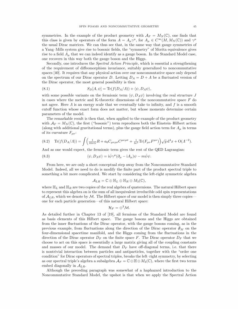
SPIN FOAMS AND NONCOMMUTATIVE GEOMETRY 45
symmetries. In the example of the product geometry with AF = MN (C), one finds thatthis class is given by operators of the form A = Aµγ
µ, for Aµ ∈ C∞(M,MN (C)) and γµ
the usual Dirac matrices. We can thus see that, in the same way that gauge symmetries ofa Yang–Mills system give rise to bosonic fields, the “symmetry” of Morita equivalence givesrise to a field Aµ that we can indeed identify as a gauge boson. In the Standard Model case,one recovers in this way both the gauge boson and the Higgs.
Secondly, one introduces the Spectral Action Principle, which is essential a strengtheningof the requirement of diffeomorphism invariance, suitably generalized to noncommutativespaces [40]. It requires that any physical action over our noncommutative space only dependon the spectrum of our Dirac operator D. Letting DA = D + A be a fluctuated version ofthe Dirac operator, the most general possibility is then
(8.1) SD[A,ψ] = Tr(f(DA/Λ)) + 〈ψ,DAψ〉,with some possible variants on the fermionic term 〈ψ,DAψ〉 involving the real structure Jin cases where the metric and K-theoretic dimensions of the noncommutative space F donot agree. Here Λ is an energy scale that we eventually take to infinity, and f is a smoothcutoff function whose exact form does not matter, but whose moments determine certainparameters of the model.
The remarkable result is then that, when applied to the example of the product geometrywith AF = MN (C), the first (“bosonic”) term reproduces both the Einstein–Hilbert action(along with additional gravitational terms), plus the gauge field action term for Aµ in termsof its curvature Fµν :
(8.2) Tr(f(DA/Λ)) =
∫ (1
16πGR+ a0CµνρσCµνρσ + 1
4e2 Tr(FµνFµν))√
g d4x+ O(Λ−2).
And as one would expect, the fermionic term gives the rest of the QED Lagrangian:
(8.3) 〈ψ,DAψ〉 = iψγµ(∂µ − iAµ)ψ −mψψ.
From here, we are only a short conceptual step away from the Noncommutative StandardModel. Indeed, all we need to do is modify the finite part of the product spectral triple tosomething a bit more complicated. We start by considering the left-right symmetric algebra
ALR = C⊕HL ⊕HR ⊕M3(C),
where HL and HR are two copies of the real algebra of quaternions. The natural Hilbert spaceto represent this algebra on is the sum of all inequivalent irreducible odd spin representationsof ALR, which we denote byM. The Hilbert space of our model is then simply three copies—one for each particle generation—of this natural Hilbert space:
HF = ⊕3M.
As detailed further in Chapter 13 of [19], all fermions of the Standard Model are foundas basis elements of this Hilbert space. The gauge bosons and the Higgs are obtainedfrom the inner fluctuations of the Dirac operator, with the gauge bosons coming, as in theprevious example, from fluctuations along the direction of the Dirac operator /∂M on thefour-dimensional spacetime manifold, and the Higgs coming from the fluctuations in thedirection of the Dirac operator DF on the finite space F . The Dirac operator DF that wechoose to act on this space is essentially a large matrix giving all of the coupling constantsand masses of our model. The demand that DF have off-diagonal terms, i.e. that thereis nontrivial interaction between particles and antiparticles, together with the “order onecondition” for Dirac operators of spectral triples, breaks the left–right symmetry, by selectingas our spectral triple’s algebra a subalgebra AF = C⊕H⊕M3(C), where the first two termsembed diagonally in ALR.
Although the preceding paragraph was somewhat of a haphazard introduction to theNoncommutative Standard Model, the upshot is that when we apply the Spectral Action
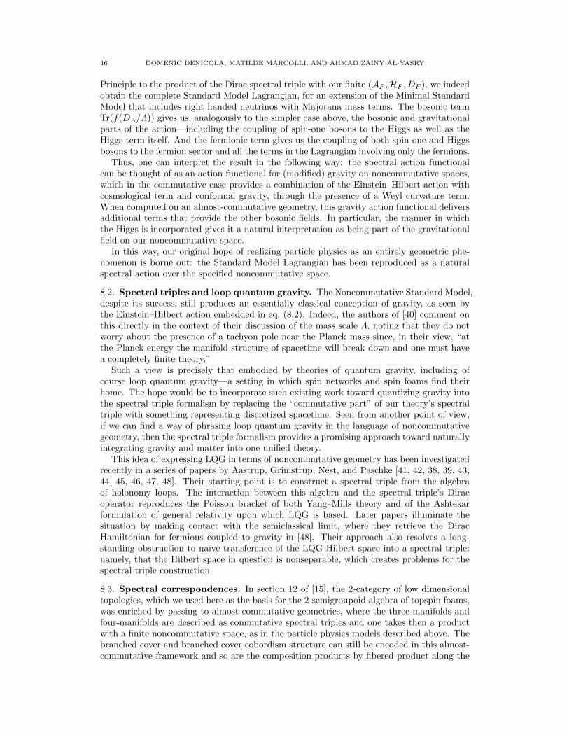
46 DOMENIC DENICOLA, MATILDE MARCOLLI, AND AHMAD ZAINY AL-YASRY
Principle to the product of the Dirac spectral triple with our finite (AF ,HF , DF ), we indeedobtain the complete Standard Model Lagrangian, for an extension of the Minimal StandardModel that includes right handed neutrinos with Majorana mass terms. The bosonic termTr(f(DA/Λ)) gives us, analogously to the simpler case above, the bosonic and gravitationalparts of the action—including the coupling of spin-one bosons to the Higgs as well as theHiggs term itself. And the fermionic term gives us the coupling of both spin-one and Higgsbosons to the fermion sector and all the terms in the Lagrangian involving only the fermions.
Thus, one can interpret the result in the following way: the spectral action functionalcan be thought of as an action functional for (modified) gravity on noncommutative spaces,which in the commutative case provides a combination of the Einstein–Hilbert action withcosmological term and conformal gravity, through the presence of a Weyl curvature term.When computed on an almost-commutative geometry, this gravity action functional deliversadditional terms that provide the other bosonic fields. In particular, the manner in whichthe Higgs is incorporated gives it a natural interpretation as being part of the gravitationalfield on our noncommutative space.
In this way, our original hope of realizing particle physics as an entirely geometric phe-nomenon is borne out: the Standard Model Lagrangian has been reproduced as a naturalspectral action over the specified noncommutative space.
8.2. Spectral triples and loop quantum gravity. The Noncommutative Standard Model,despite its success, still produces an essentially classical conception of gravity, as seen bythe Einstein–Hilbert action embedded in eq. (8.2). Indeed, the authors of [40] comment onthis directly in the context of their discussion of the mass scale Λ, noting that they do notworry about the presence of a tachyon pole near the Planck mass since, in their view, “atthe Planck energy the manifold structure of spacetime will break down and one must havea completely finite theory.”
Such a view is precisely that embodied by theories of quantum gravity, including ofcourse loop quantum gravity—a setting in which spin networks and spin foams find theirhome. The hope would be to incorporate such existing work toward quantizing gravity intothe spectral triple formalism by replacing the “commutative part” of our theory’s spectraltriple with something representing discretized spacetime. Seen from another point of view,if we can find a way of phrasing loop quantum gravity in the language of noncommutativegeometry, then the spectral triple formalism provides a promising approach toward naturallyintegrating gravity and matter into one unified theory.
This idea of expressing LQG in terms of noncommutative geometry has been investigatedrecently in a series of papers by Aastrup, Grimstrup, Nest, and Paschke [41, 42, 38, 39, 43,44, 45, 46, 47, 48]. Their starting point is to construct a spectral triple from the algebraof holonomy loops. The interaction between this algebra and the spectral triple’s Diracoperator reproduces the Poisson bracket of both Yang–Mills theory and of the Ashtekarformulation of general relativity upon which LQG is based. Later papers illuminate thesituation by making contact with the semiclassical limit, where they retrieve the DiracHamiltonian for fermions coupled to gravity in [48]. Their approach also resolves a long-standing obstruction to naıve transference of the LQG Hilbert space into a spectral triple:namely, that the Hilbert space in question is nonseparable, which creates problems for thespectral triple construction.
8.3. Spectral correspondences. In section 12 of [15], the 2-category of low dimensionaltopologies, which we used here as the basis for the 2-semigroupoid algebra of topspin foams,was enriched by passing to almost-commutative geometries, where the three-manifolds andfour-manifolds are described as commutative spectral triples and one takes then a productwith a finite noncommutative space, as in the particle physics models described above. Thebranched cover and branched cover cobordism structure can still be encoded in this almost-commutative framework and so are the composition products by fibered product along the
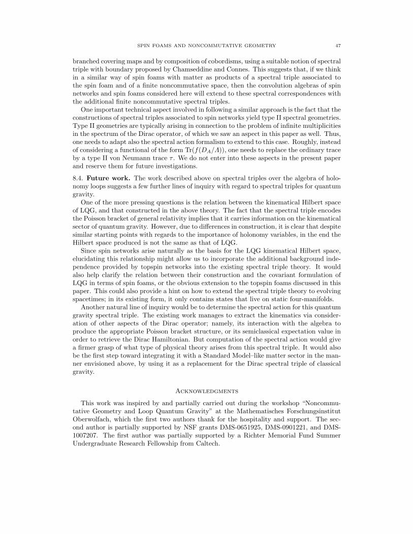
SPIN FOAMS AND NONCOMMUTATIVE GEOMETRY 47
branched covering maps and by composition of cobordisms, using a suitable notion of spectraltriple with boundary proposed by Chamseddine and Connes. This suggests that, if we thinkin a similar way of spin foams with matter as products of a spectral triple associated tothe spin foam and of a finite noncommutative space, then the convolution algebras of spinnetworks and spin foams considered here will extend to these spectral correspondences withthe additional finite noncommutative spectral triples.
One important technical aspect involved in following a similar approach is the fact that theconstructions of spectral triples associated to spin networks yield type II spectral geometries.Type II geometries are typically arising in connection to the problem of infinite multiplicitiesin the spectrum of the Dirac operator, of which we saw an aspect in this paper as well. Thus,one needs to adapt also the spectral action formalism to extend to this case. Roughly, insteadof considering a functional of the form Tr(f(DA/Λ)), one needs to replace the ordinary traceby a type II von Neumann trace τ . We do not enter into these aspects in the present paperand reserve them for future investigations.
8.4. Future work. The work described above on spectral triples over the algebra of holo-nomy loops suggests a few further lines of inquiry with regard to spectral triples for quantumgravity.
One of the more pressing questions is the relation between the kinematical Hilbert spaceof LQG, and that constructed in the above theory. The fact that the spectral triple encodesthe Poisson bracket of general relativity implies that it carries information on the kinematicalsector of quantum gravity. However, due to differences in construction, it is clear that despitesimilar starting points with regards to the importance of holonomy variables, in the end theHilbert space produced is not the same as that of LQG.
Since spin networks arise naturally as the basis for the LQG kinematical Hilbert space,elucidating this relationship might allow us to incorporate the additional background inde-pendence provided by topspin networks into the existing spectral triple theory. It wouldalso help clarify the relation between their construction and the covariant formulation ofLQG in terms of spin foams, or the obvious extension to the topspin foams discussed in thispaper. This could also provide a hint on how to extend the spectral triple theory to evolvingspacetimes; in its existing form, it only contains states that live on static four-manifolds.
Another natural line of inquiry would be to determine the spectral action for this quantumgravity spectral triple. The existing work manages to extract the kinematics via consider-ation of other aspects of the Dirac operator; namely, its interaction with the algebra toproduce the appropriate Poisson bracket structure, or its semiclassical expectation value inorder to retrieve the Dirac Hamiltonian. But computation of the spectral action would givea firmer grasp of what type of physical theory arises from this spectral triple. It would alsobe the first step toward integrating it with a Standard Model–like matter sector in the man-ner envisioned above, by using it as a replacement for the Dirac spectral triple of classicalgravity.
Acknowledgments
This work was inspired by and partially carried out during the workshop “Noncommu-tative Geometry and Loop Quantum Gravity” at the Mathematisches ForschungsinstitutOberwolfach, which the first two authors thank for the hospitality and support. The sec-ond author is partially supported by NSF grants DMS-0651925, DMS-0901221, and DMS-1007207. The first author was partially supported by a Richter Memorial Fund SummerUndergraduate Research Fellowship from Caltech.
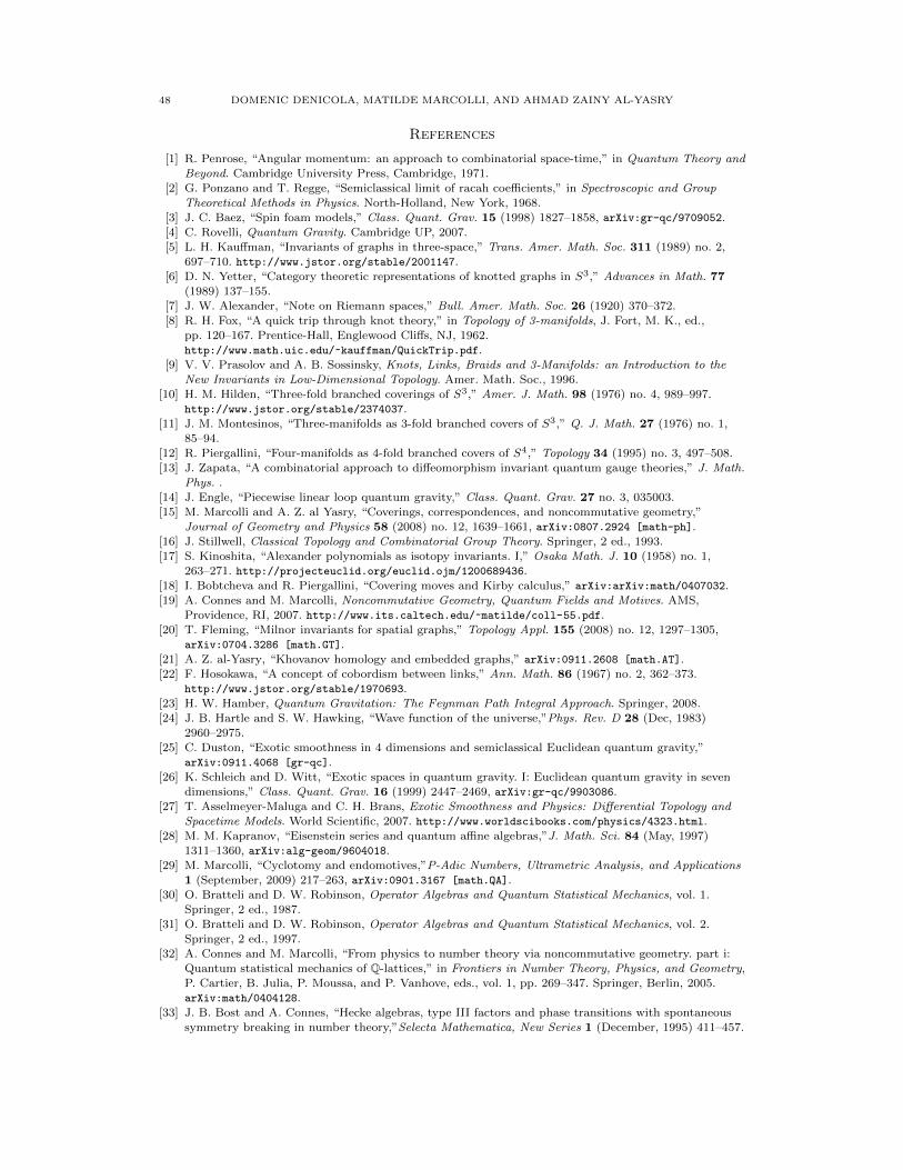
48 DOMENIC DENICOLA, MATILDE MARCOLLI, AND AHMAD ZAINY AL-YASRY
References
[1] R. Penrose, “Angular momentum: an approach to combinatorial space-time,” in Quantum Theory and
Beyond. Cambridge University Press, Cambridge, 1971.[2] G. Ponzano and T. Regge, “Semiclassical limit of racah coefficients,” in Spectroscopic and Group
Theoretical Methods in Physics. North-Holland, New York, 1968.[3] J. C. Baez, “Spin foam models,” Class. Quant. Grav. 15 (1998) 1827–1858, arXiv:gr-qc/9709052.
[4] C. Rovelli, Quantum Gravity. Cambridge UP, 2007.
[5] L. H. Kauffman, “Invariants of graphs in three-space,” Trans. Amer. Math. Soc. 311 (1989) no. 2,697–710. http://www.jstor.org/stable/2001147.
[6] D. N. Yetter, “Category theoretic representations of knotted graphs in S3,” Advances in Math. 77
(1989) 137–155.[7] J. W. Alexander, “Note on Riemann spaces,” Bull. Amer. Math. Soc. 26 (1920) 370–372.
[8] R. H. Fox, “A quick trip through knot theory,” in Topology of 3-manifolds, J. Fort, M. K., ed.,
pp. 120–167. Prentice-Hall, Englewood Cliffs, NJ, 1962.http://www.math.uic.edu/~kauffman/QuickTrip.pdf.
[9] V. V. Prasolov and A. B. Sossinsky, Knots, Links, Braids and 3-Manifolds: an Introduction to the
New Invariants in Low-Dimensional Topology. Amer. Math. Soc., 1996.[10] H. M. Hilden, “Three-fold branched coverings of S3,” Amer. J. Math. 98 (1976) no. 4, 989–997.
http://www.jstor.org/stable/2374037.[11] J. M. Montesinos, “Three-manifolds as 3-fold branched covers of S3,” Q. J. Math. 27 (1976) no. 1,
85–94.
[12] R. Piergallini, “Four-manifolds as 4-fold branched covers of S4,” Topology 34 (1995) no. 3, 497–508.[13] J. Zapata, “A combinatorial approach to diffeomorphism invariant quantum gauge theories,” J. Math.
Phys. .
[14] J. Engle, “Piecewise linear loop quantum gravity,” Class. Quant. Grav. 27 no. 3, 035003.[15] M. Marcolli and A. Z. al Yasry, “Coverings, correspondences, and noncommutative geometry,”
Journal of Geometry and Physics 58 (2008) no. 12, 1639–1661, arXiv:0807.2924 [math-ph].
[16] J. Stillwell, Classical Topology and Combinatorial Group Theory. Springer, 2 ed., 1993.[17] S. Kinoshita, “Alexander polynomials as isotopy invariants. I,” Osaka Math. J. 10 (1958) no. 1,
263–271. http://projecteuclid.org/euclid.ojm/1200689436.
[18] I. Bobtcheva and R. Piergallini, “Covering moves and Kirby calculus,” arXiv:arXiv:math/0407032.[19] A. Connes and M. Marcolli, Noncommutative Geometry, Quantum Fields and Motives. AMS,
Providence, RI, 2007. http://www.its.caltech.edu/~matilde/coll-55.pdf.[20] T. Fleming, “Milnor invariants for spatial graphs,” Topology Appl. 155 (2008) no. 12, 1297–1305,
arXiv:0704.3286 [math.GT].
[21] A. Z. al-Yasry, “Khovanov homology and embedded graphs,” arXiv:0911.2608 [math.AT].[22] F. Hosokawa, “A concept of cobordism between links,” Ann. Math. 86 (1967) no. 2, 362–373.
http://www.jstor.org/stable/1970693.
[23] H. W. Hamber, Quantum Gravitation: The Feynman Path Integral Approach. Springer, 2008.[24] J. B. Hartle and S. W. Hawking, “Wave function of the universe,”Phys. Rev. D 28 (Dec, 1983)
2960–2975.
[25] C. Duston, “Exotic smoothness in 4 dimensions and semiclassical Euclidean quantum gravity,”arXiv:0911.4068 [gr-qc].
[26] K. Schleich and D. Witt, “Exotic spaces in quantum gravity. I: Euclidean quantum gravity in sevendimensions,” Class. Quant. Grav. 16 (1999) 2447–2469, arXiv:gr-qc/9903086.
[27] T. Asselmeyer-Maluga and C. H. Brans, Exotic Smoothness and Physics: Differential Topology andSpacetime Models. World Scientific, 2007. http://www.worldscibooks.com/physics/4323.html.
[28] M. M. Kapranov, “Eisenstein series and quantum affine algebras,”J. Math. Sci. 84 (May, 1997)
1311–1360, arXiv:alg-geom/9604018.
[29] M. Marcolli, “Cyclotomy and endomotives,”P-Adic Numbers, Ultrametric Analysis, and Applications1 (September, 2009) 217–263, arXiv:0901.3167 [math.QA].
[30] O. Bratteli and D. W. Robinson, Operator Algebras and Quantum Statistical Mechanics, vol. 1.Springer, 2 ed., 1987.
[31] O. Bratteli and D. W. Robinson, Operator Algebras and Quantum Statistical Mechanics, vol. 2.
Springer, 2 ed., 1997.
[32] A. Connes and M. Marcolli, “From physics to number theory via noncommutative geometry. part i:Quantum statistical mechanics of Q-lattices,” in Frontiers in Number Theory, Physics, and Geometry,
P. Cartier, B. Julia, P. Moussa, and P. Vanhove, eds., vol. 1, pp. 269–347. Springer, Berlin, 2005.arXiv:math/0404128.
[33] J. B. Bost and A. Connes, “Hecke algebras, type III factors and phase transitions with spontaneous
symmetry breaking in number theory,”Selecta Mathematica, New Series 1 (December, 1995) 411–457.
SPIN FOAMS AND NONCOMMUTATIVE GEOMETRY 49
[34] A. H. Chamseddine, A. Connes, and M. Marcolli, “Gravity and the Standard Model with neutrinomixing,” Adv. Theor. Math. Phys. 11 (2007) 991–1089, arXiv:hep-th/0610241.
[35] A. Connes and G. Skandalis, “The longitudinal index theorem for foliations,” Publ. Res. Inst. Math.
Sci. 20 (1984) no. 6, 1139–1183.[36] J. Brodzki, V. Mathai, J. Rosenberg, and R. J. Szabo, “Noncommutative correspondences, duality
and D-branes in bivariant K-theory,” Adv. Theor. Math. Phys. 13 (2009) 497–552, arXiv:0708.2648
[hep-th].[37] P. Bouwknegt, K. Hannabuss, and V. Mathai, “Nonassociative tori and applications to T-duality,”
Commun. Math. Phys. 264 (2006) 41–69, arXiv:hep-th/0412092.[38] J. Aastrup, J. M. Grimstrup, and R. Nest, “On spectral triples in quantum gravity I,” Class. Quant.
Grav. 26 (2009) 065011, arXiv:0802.1783 [hep-th].
[39] J. Aastrup, J. M. Grimstrup, and R. Nest, “On spectral triples in quantum gravity II,” J.Noncommut. Geom. 3 (2009) 47–81, arXiv:0802.1784 [hep-th].
[40] A. H. Chamseddine and A. Connes, “The spectral action principle,” Commun. Math. Phys. 186
(1997) 731–750, arXiv:hep-th/9606001.[41] J. Aastrup and J. M. Grimstrup, “Spectral triples of holonomy loops,” Commun. Math. Phys. 264
(2006) 657–681, arXiv:hep-th/0503246.
[42] J. Aastrup and J. M. Grimstrup, “Intersecting Connes noncommutative geometry with quantumgravity,” Int. J. Mod. Phys. A22 (2007) 1589, arXiv:hep-th/0601127.
[43] J. Aastrup, J. M. Grimstrup, and R. Nest, “A new spectral triple over a space of connections,”
Commun. Math. Phys. 290 (2009) 389–398, arXiv:0807.3664 [hep-th].[44] J. Aastrup, J. M. Grimstrup, and R. Nest, “Holonomy loops, spectral triples & quantum gravity,”
Class. Quant. Grav. 26 (2009) 165001, arXiv:0902.4191 [hep-th].[45] J. Aastrup, J. M. Grimstrup, M. Paschke, and R. Nest, “On semi-classical states of quantum gravity
and noncommutative geometry,” arXiv:0907.5510 [hep-th].
[46] J. Aastrup, J. M. Grimstrup, and M. Paschke, “Emergent Dirac hamiltonians in quantum gravity,”arXiv:0911.2404 [hep-th].
[47] J. Aastrup and J. M. Grimstrup, “Lattice loop quantum gravity,” arXiv:0911.4141 [gr-qc].
[48] J. Aastrup, J. M. Grimstrup, and M. Paschke, “On a derivation of the Dirac Hamiltonian from aconstruction of quantum gravity,” arXiv:1003.3802 [hep-th].
E-mail address: [email protected]
E-mail address: [email protected]
E-mail address: [email protected]
MSC #240, California Institute of Technology, 1200 E. California Blvd., Pasadena, CA 91126,USA
Division of Physics, Mathematics, and Astronomy, California Institute of Technology, 1200
E. California Blvd., Pasadena, CA 91125, USA
Abdus Salam International Center for Theoretical Physics, Strada Costiera 11, Trieste,
I-34151, Italy


![S-Dualities in noncommutative and nonanticommutative field ... F-Dayi.pdf · Noncommutative space is defined by constant B : [XIL, XV] = BILv Duality can be generalized to noncommutative](https://static.fdocuments.us/doc/165x107/605cc47844073f56bf09ce8c/s-dualities-in-noncommutative-and-nonanticommutative-field-f-dayipdf-noncommutative.jpg)