Spillovers, disclosure lags, and incentives to … · Spillovers, disclosure lags, and incentives...

Spillovers, disclosure lags, and incentives toinnovate: Do oligopolies over-invest in R&D?

Gianluca Femminisx� and Gianmaria Martini+

October 2007

xCatholic University of Milan, Italy

+University of Bergamo, Italy

Abstract

We develop a dynamic duopoly, where �rms have to take into account atechnological externality, that reduces over time their innovation costs,and an inter-�rm spillover, that lowers only the second comer�s R&Dcost. This spillover exerts its e¤ect after a disclosure lag. We identifythree possible equilibria, which are classi�ed, according to the timingof R&D investments, as early, intermediate, and late. The intermedi-ate equilibrium is subgame perfect for a wide parameters range. Whenthe innovation size is large, it implies that the duopolistic market equi-librium involves underinvestment. Hence, even in presence of a mod-erate degree of inter-�rms spillover, the competitive equilibrium callsfor public policies aimed at increasing the research activity. When wefocus on minor innovations �the case in which, according to the ear-lier literature, the market equilibrium underinvests �our results implythat the policies aimed at stimulating R&D have to be less sizeablethan suggested before, despite the presence of an inter-�rm spillover.

JEL classi�cation: L13, L41, O33Keywords: R&D, knowledge spillover, dynamic oligopoly

�Correspondence to: G. Femminis, ITEMQ, Università Cattolica di Milano, LargoGemelli 1, 20123 Milano, ITALY, email: [email protected]. We thank PieroTedeschi for helpful comments and suggestions. Preliminary versions of this paper havebeen presented at the Royal Economic Society 2007 Conference, and at the 5th IIOCAnnual Conference, and in various Universities. Usual disclaimers apply.

1

1 Introduction

Understanding �rms�decision to innovate is of fundamental importance todesign policies aimed at maximizing welfare. The �rms�decisions are drivenby their incentives; hence the market structure in which �rms operate playsa crucial role in determining the pace of technical progress. This provides astrong motivation for the analysis of oligopolies, which are the most wide-spread market con�guration.

In our study, we analyze a duopoly in which �as in many recent contri-butions (e.g. Stenbacka and Tombak (1994), Hoppe (2000), and Schmidt-Dengler (2006)) �the R&D cost shrinks over time thanks to general advancesin knowledge and technology. In addition to this standard technological ex-ternality, �rms take into account a spillover that lowers the second comer�sinnovation cost. A distinctive features of our duopoly game is that thespillover exerts its e¤ect after a time period which we label �disclosure lag�.

When the oligopolistic competition is driven by the innovative activity,inter-�rm spillovers play an important role. In fact, they alter the length ofthe follower�s strategic delay, and hence the leader�s cost advantage period.1

Also the presence of a disclosure lag has important strategic implications.In fact, the �rst innovator is aware that the second comer cannot exploit thespillovers before the relevant information are disclosed. Hence, the behaviorof the interacting �rms is in�uenced by the existence of a production cost-advantage period for the �rst comer.

What we �nd is that in our framework three types of equilibria arise,while the existing contributions, following Fudenberg and Tirole (1985),identi�es two possible market equilibria: an early and a late one.

This literature, which starts with Reinganum (1981), and is excellentlysurveyed by Hoppe (2002), identi�es two driving forces characterizing theequilibria: the length of the follower�s strategic delay, and the intensity ofthe competitive pressure. In the early equilibrium, the second innovatordelays his decision to invest for a relatively long period. This choice isdriven by the desire to grasp the bene�t of technical progress, that reducesthe innovation cost as time goes by. The follower�s optimal choice impliesa long competitive advantage period for the innovator leader, which favorsthe latter�s payo¤ at the expenses of the former�s one. Hence, to avoid beingpreempted, the �rst mover invests �very soon�, and the R&D investment issocially excessive. The preemption possibility also implies rent equalization.

1The importance of spillovers for R&D is underscored in De Bondt (1996), who providesmany reference to earlier contributions, which, however, adopt static even if multi-stageframeworks.

1

In contrast, a late equilibrium arises once technical progress has substantiallyreduced the innovation costs, so that an innovation leader cannot emerge,because the rival would immediately copy her decision. In this case, anyinnovator �anticipating that there will be no leadership �waits until herchoice maximizes the joint discounted stream of net pro�ts. The collusive�avour of this equilibrium is apparent: accordingly, Fudenberg and Tirole�sanalysis implies that this type of market equilibrium underinvests. Theircontribution also suggests that the early equilibrium is subgame perfectwhen the size of the innovation is large. In this case, in fact, the per-period �rst innovator pro�ts are considerable, which triggers the preemptivebehavior.

We label �intermediate�the third type of equilibrium we identify, sincethe decisions to innovate take place, for both �rms, at dates positioned be-tween the early and the late ones. This happens because the �rst innovatorknows that the second comer will exploit the spillovers as soon as the rel-evant information is obtained, i.e. exactly at the end of the disclosure lag.Because in the early equilibrium the follower waits more than the disclosurelag, the leader�s competitive advantage period is shorter in the intermedi-ate equilibrium than in the early one. This harms the leader�s discountedpro�ts, but the follower is bene�ted. Therefore the competitive pressure �that leads to rent equalization�is weaker than in the early equilibrium, anddoes not force the leader to invest �very soon�. However, the competitivepressure is high enough to avoid a late equilibrium.

We select the equilibrium for the overall game by applying the subgameperfection criterion, and we �nd that the intermediate equilibrium is par-ticularly relevant because it is the prevailing one for a large range of theparameters set. Notice that � in our framework � the natural indicatorsof an highly competitive environment, namely an equilibrium with R&Ddi¤usion and rent equalization, do not imply that the R&D investment isexcessive from the social planner�s perspective.

When the innovation size is large, the intermediate equilibrium impliesthat the duopolistic market equilibrium involves underinvestment. An un-derinvesting equilibrium in presence of a major innovation is a result thatcontrasts not only with the literature following Fudenberg and Tirole, butalso with the previous contributions inspired by Loury (1979), and by Leeand Wilde (1980).2 The relevant implication is that, according to our model,

2Loury, and Lee and Wilde assume that a new technique becomes suddenly available,and immediately triggers the industry investment in R&D. The competitive pressure in-duced by the market structure implies that the equilibrium involves an R&D investmentthat is higher than the social optimum. This result can partially be ascribed to the tourna-

2

the competitive equilibrium calls for public policies aimed at increasing theresearch activity.

When, instead, we focus on minor innovations, the equilibrium we de-scribe is more realistic than the late one, which is characterized by simulta-neous adoptions, a phenomenon seldom observed in the real world. Noticethat, with minor innovations � the case in which, according to the earlierliterature, the market equilibrium underinvests �the prevalence of the in-termediate equilibrium imply that the policies aimed at stimulating R&Dhave to be less sizeable than suggested before, despite the presence of aninter-�rm spillover.

To understand why the intermediate equilibrium is subgame perfect,consider �rst the case of an innovation of limited size. In this situation,when the spillover is (relatively) high, the follower grasps (relatively) largebene�ts from investing at the end of the disclosure lag, so that he �ndsoptimal to select this strategy for a long time interval. This makes theleader unwilling to wait until the late equilibrium prevails, which gives riseto the intermediate equilibrium. When, instead, the spillover is very low,the subgame perfect equilibrium is the late one, because the �immediatereply�strategy for the follower becomes optimal at earlier dates.3

In contrast, when the innovation size is large, an early equilibrium mayemerge, because a major innovation, bringing a large cost advantage to theleader, enhances her incentive to be �rst. However, the higher the spillover,the sooner the second comer �due to the reduction in innovation costs �optimally invests in reply to an early leader�s investment. This reducesthe leaders� e¢ ciency advantage period, leading to the dominance of theintermediate equilibrium. Moreover, a (relatively) high spillover increasesthe second comer�s payo¤ in the intermediate time interval, and this softensthe leader�s preemption incentive to invest. This milder competition implieshigher payo¤s for both �rms in the intermediate equilibrium.

These results, being driven by the assumption of an inter-�rm spillovercoupled with the one of a disclosure lag, di¤er from the ones already obtainedin the literature. In fact, Riordan (1992) focuses on the early equilibrium,and analyses the impact of price and entry regulations on the timing of

ment nature of these models. In a non-tournament model, Beath et al (1989) underscorethe role of the competitive threat as a major determinant of R&D expenditure. Becausethe larger is the competitive threat, the more resources �rms invest in R&D, overinvest-ment is more likely, the larger is the size of the innovation. Delbono and Denicolò (1991),again in a non-tournament framework, �nd that the equilibrium R&D e¤ort can be lowerthan the social optimum if the marginal cost of the innovation is low.

3As in the previous literature, a small cost reduction, implying a weak incentive toinnovate �rst, does not give rise to an equilibrium with preemption.

3

adoption. Because these regulatory schemes tend to reduce the �rst innova-tor�s rents, they are likely to delay the early adoption, which can be sociallybene�cial.

Stenbacka and Tomback (1994) analyze the role of experience, whichimplies that the probability of successful implementation of an innovationis an increasing function of the time distance from the investment date.As for welfare, they show that a collusive adoption timing may improvewelfare when compared with the market equilibrium. This happens whenthe pace of technical progress is fairly high: when this is the case, a collusiveadoption is bene�cial because the industry can fully take advantage of thereduction of innovation cost. In contrast, a competitive market equilibrium,being driven by the incentives to obtain a strategic advantage, induces apremature adoption.

In Hoppe (2000), �rms are uncertain about the pro�tability of the inno-vation. Her framework di¤ers from the one by Fudenberg and Tirole, thanksto the presence of technological uncertainty, which induces an asymmetrybetween the leader and the follower. The latter observes the leader�s out-come, and hence becomes aware about the actual pro�tability characterizingthe new technique. This informational spillover may bring about a second-mover advantage. Moreover, an high probability of failure induces a latesimultaneous adoption because it curtails the �rst mover expected payo¤.When the late equilibrium is subgame perfect, Hoppe �nds that an earliersimultaneous adoption would be welfare increasing, while the result are lessde�nite when the early equilibrium prevails.

Weeds (2002) presents a tournament version of Fudenberg and Tirole(1985), in which pro�ts evolve stochastically. She suggests that the early(late) equilibrium over(under)-invests; however the late equilibrium is closerto the social optimum than the early one.4

The paper proceeds in the standard way. In Section 2 we present ourmodel. In Section 3 we discuss the equilibrium concept adopted in theanalysis and we compute the di¤erent market equilibria, in which �rmscompete both in the innovation and in the product stages. Then, subgame

4The presence of an inter-�rm spillover assimilates our model to the frameworks pro-posed by Katz and Shapiro (1987), Dutta et al. (1995), and Hoppe and Lehmann-Gruber(2005) among others. Katz and Shapiro introduce an extreme form of technologicalspillover, assuming that, in a duopoly, the follower can adopt at no cost the new tech-nology as soon as the leader has invested. This hypothesis induces the possibility of asecond mover advantage. A similar approach is followed in Dasgupta (1988). Dutta et al.demonstrate that the second mover advantage may prevail as subgame perfect equilibriumoutput in product innovation games. Hoppe and Lehmann-Gruber generalize the previousresults by analyzing the issue of multiple peaks in the leader�s payo¤ function.

4

perfectness is invoked as a selection device among market equilibria. InSection 4 we spell out the welfare implications of our analysis. Concludingcomments in Section 5 end the paper.

2 The model

2.1 The production stage and its welfare implications

We consider an industry composed of two �rms, 1 and 2, which, in each(in�nitesimally short) period, are involved in a two�stage interaction: �rstthey decide whether to innovate or not, and then they compete à la Cournot.Time is continuous and �rms� horizon is in�nite. Firms discount futurepro�ts at the common rate r. Market demand is linear and equal to: P =a � bQ, where P is the market clearing price and Q = q1 + q2 is the totalquantity supplied. Each �rm has a unit cost of production c.

The R&D cost evolves over time.5 In each period t �rm i (i = 1; 2)decides whether to invest in R&D or not. This investment immediatelyyields a cost-reducing process innovation, which shrinks the unit productioncost by an amount x, with x < c. Hence �rm i�s post�innovation productioncost is C(qi) = (c� x)qi.

Each �rm�s payo¤ will depend not only on its adoption date but also onits rival�s one. If both �rms have not invested up to period t, their individualpro�ts in the Cournot subgame at t are those of the pre�innovation stage,i.e.

�00i =A2

9b; (1)

where A = a � c: The superscript f00g indicates that both �rms do notinnovate at t: The instantaneous welfare (computed à la Marshall) is thenequal to:

W 00 =4

9

A2

b: (2)

If instead only one �rm, say �rm 1; invests in R&D at t, it bene�ts ofan e¢ ciency advantage, and obtains a higher market share. The marketprice at t decreases in comparison with the pre-innovation level, while theindividual pro�ts become:

5The functional forms and dynamics for the �rms�R&D costs are modeled in Section2.2.

5

�101 =(A+ 2x)2

9b;�102 =

(A� x)29b

; (3)

where f10g indicates that �rm 1 has invested in R&D while �rm 2 has not.Notice that �101 > �102 ; �

101 > �001 and �102 < �002 : Because q

102 = A�x

3b ;

to preserve the duopolistic structure characterizing our market we need tointroduce:

Assumption 1: A > x.This hypothesis implies that, in a Cournot environment, the cost-reducing

innovation is non�drastic (see, Denicolò (1996)). In case of asymmetric be-havior at t, welfare is:

W 10 =8A(A+ x) + 11x2

18b; (4)

with W 10 > W 00:

Finally, we need to compute the outcomes when both �rms have inno-vated at t. In this case, being more e¢ cient, they both produce more thanin the status quo; therefore, the market price is lower. Individual pro�ts att are:

�11i =(A+ x)2

9b; (5)

where the superscript f11g indicates that both �rms have innovated.Obviously, �101 > �111 ; notice, moreover, that the di¤erence between �

101

and �111 is increasing in x: when only one �rm enjoys a cost advantage, sheobtains a larger market share while bene�ting from an higher price to costmargin.

When both �rms have innovated, the social welfare is:

W 11 =4(A+ x)2

9b; (6)

with W 11 > W 10 (by Assumption 1).When �rms simultaneously invest in R&D, individual pro�ts rise from

(1) to (5) and welfare jumps from (2) to (6). Alternatively, �rms may behaveasymmetrically, so that there are both an innovation leader and a follower.Under these circumstances individual pro�ts �rst change from to (1) to (3)(and welfare from (2) to (4)) and then from (3) to (5) (and welfare from (4)to (6)).

6

2.2 R&D costs

In our set-up, �rms decides whether to invest in a �xed-size research project.For the �rst �rm investing in R&D, the innovation cost evolves over timeaccording to the following equation:

C1(t1) = xe��(t1�t0); for t1 2 [t0;1); (7)

where t1 is the calendar time when the �rst �rm has introduced the inno-vation. Hence, we are assuming that the innovation becomes technicallyfeasible at time t0 at a cost, x, which then decreases at the constant rate� � 0; thanks to the advances in pure research and to the availability of newresults obtained in related �elds. Of course, this form of technical progressis exogenous to any single �rm. It is clear from (7) that, if a �rm innovatesin period t, R&D costs are sunk at that time.

As for the second �rm introducing the innovation, the cost evolution isdescribed by the following equation:

C2(t2) =

� xe��(t2�t0) for t2 2 [t1; t1 +�)(1� �) xe��(t2�t0) for t2 2 [t1 +�;1)

; (8)

where � 2 [0; ��] is the inter-�rm spillover parameter; �� shall be assumed asbeing strictly lower than unity. In fact, with � = 1, the follower �bearingno innovation cost �would always invest at the end of the disclosure lag.Hence, this (irrealistic) particular case would deliver trivial results. � isthe delay needed to grasp the bene�t stemming from the rival�s innovativeactivity. Hence, � is the exogenously determined disclosure lag.

Whenever � > 0 the innovation is only partially appropriable: the secondcomer enjoys a reduction in R&D costs by imitating his competitor at t2 �t1 + �. In our formulation, it takes time to imitate an innovation: in hisclassic study, Mans�eld (1985) reports that in 59% of cases it takes more thantwelve months to the innovator�s rival to obtain the relevant information.More recently, Cohen et al. (2002) compute that the average adoption lag forunpatented process innovation is 2.03 and 3.37 years in Japan and in the US,respectively. An obvious but important consequence of our assumption isthat the introduction of an innovation grants to the leader a cost advantage(and hence higher pro�ts) for a time period (at least) equal to �.

We stylize an extremely simple form of spillover: it would have beenpreferable to consider a stochastic disclosure lag, with a probability of in-formation di¤usion depending upon the time elapsed from the introductionof the innovation, and on the follower�s imitation e¤ort. The latter should

7

be used to in�uence also the spillover size.6 However, even the simpleststochastic formulation � namely the one involving a constant probabilityof information di¤usion coupled with a �xed spillover size �precludes theattainment of explicit results.7 Hence, our formulation has been chosen asthe optimal compromise between analytical tractability and �realism�.

In what follows we will restrict the values for �; � and : In particular,we now introduce the following technical assumptions:

Assumption 2: max�

xA+x ; 1�

4A6A+3x

�1 + r

�2A+3x6A+3x

� �r

�� < 1:

Assumption 3: � � �� = 1r ln

�1 + r

�2A+3x6A+3x

�;

Assumption 4: � � = 4A exp(� ��)

9b(r+�)(1��) :

Assumption 2 allows for su¢ ciently high spill-over levels, which makesthe discussion more interesting.

The purpose of Assumption 3 is to limit the number of cases that we needto consider. To verify that Assumption 3 does not restrict � to values tooshort to be sensible, we compute �� when x approaches 0 (since this choicelowers ��); the annual interest rate is 0.03, and � = {0.01, 0.05, 0.09}.8

With these values, �� becomes, respectively, equal to {23.105, 6.077, 3.512}.Hence, the restriction implied by Assumption 3 is realistic in most contexts.From the vantage point of economic analysis, a low � is interesting, becauseit makes more relevant the role of the inter-�rms spillovers.

Assumption 4 guarantees the existence of all the three types of equilibriain the space [0; ��] x [0; ��]:

3 The market equilibria

In this Section we discuss the equilibria in the non-cooperative R&D game.To this purpose, we �rst explain the equilibrium concept adopted to solvethe model. Because the payo¤ functions, in general, are not single-peaked,we deal with the existence of multiple equilibria. We divide time in threesub-intervals, in such a way that in each interval the equilibrium is unique.

6To endogenize � we could have followed Jin and Troege (2006), which suggest that�rms can raise it, paying a convex imitation cost. Nevertheless, we preferred not topursue this development of the model, because our framework is already fairly complex:any further extension requires a much heavier use of numerical techniques to determineand select the equilibrium. For the same reason we do not endogenize the lenght of thedisclosure lag.

7Notice also that a constant probability of information disclosure does not represent animprovement upon our formulation, since the sparse empirical evidence available suggeststhat the probability of successful imitation increases over time.

8These values for � have a relevant economic interpretation that will become apparentlater.

8

We then select the globally unique equilibrium referring to the concept ofsubgame perfectness.

3.1 The equilibrium concept

As already mentioned, in our set-up only one research project is available tothe �rms: hence, the choice to innovate at time ti is an irreversible stoppingdecision. Therefore, our model belongs to the class of symmetric timinggames, which can be divided into two sub-classes, depending upon which�rm (the one that moves �rst or the one that moves second) obtains thehigher payo¤.

We can make this point more precise, by assuming for the moment thatwe have exogenously assigned the task of moving �rst to one of the two�rms. In this case, there is a �rst mover advantage if the �rm that mustmove �rst obtains the higher payo¤. If, instead, the �rst mover obtains thelower payo¤, there is a second mover advantage. Obviously the �rst mover isassumed to behave optimally, choosing the innovation time that maximizesits payo¤, given the second mover optimal choice.

To deal with �rst mover advantage games, we drop the hypothesis ofexogenously assigned roles and we follow Hoppe and Lehman-Gruber (2005)assuming that:

Assumption 5: If the two �rms are indi¤erent between being the �rst orthe second mover at any date t, then the role of the leader is played by the�rm with a female CEO9 and the role of the follower is played by the other�rm, which is run by a male CEO.

Assumption 5 is used to rule out, as it happens in most of the literature,the possibility of coordination failures as an equilibrium outcome. In otherwords, �rms do not choose to move at the same instant of time if they knowthat they would regret this choice afterwards.10

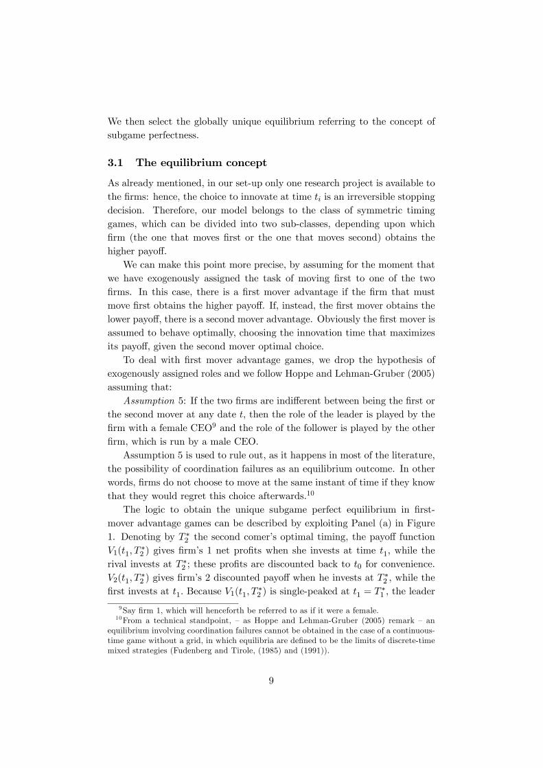
The logic to obtain the unique subgame perfect equilibrium in �rst-mover advantage games can be described by exploiting Panel (a) in Figure1. Denoting by T �2 the second comer�s optimal timing, the payo¤ functionV1(t1; T

�2 ) gives �rm�s 1 net pro�ts when she invests at time t1; while the

rival invests at T �2 ; these pro�ts are discounted back to t0 for convenience.V2(t1; T

�2 ) gives �rm�s 2 discounted payo¤ when he invests at T

�2 ; while the

�rst invests at t1: Because V1(t1; T�2 ) is single-peaked at t1 = T

�1 ; the leader

9Say �rm 1, which will henceforth be referred to as if it were a female.10From a technical standpoint, � as Hoppe and Lehman-Gruber (2005) remark � an

equilibrium involving coordination failures cannot be obtained in the case of a continuous-time game without a grid, in which equilibria are de�ned to be the limits of discrete-timemixed strategies (Fudenberg and Tirole, (1985) and (1991)).

9

would like to adopt �rst at T �1 : But the roles of innovation leader and followerare not pre-assigned. Hence, when the second �rm knows that the other willadopt at time T �1 , it is in his interest to preempt at time T

�1�dt. By backward

induction, we conclude that the equilibrium strategy for the �rst innovatoris to invest as soon as the leader�s payo¤ is equal to the follower�s one (i.e.at T¯ 1). (Assumption 5 grants us that the �rst innovator is actually �rm 1.)

Notice that the preemption argument spelled out above yields equal payo¤sto the two �rms in the subgame perfect equilibrium. Hence, in this case theequilibrium involves rent dissipation.

[Figure 1 about here]

In dealing with second mover advantage games, we rely again on Hoppeand Lehman-Gruber�s analysis. In this case, they assume that the equilib-rium is driven by expectations and make the following hypothesis:

Assumption 6: Whenever the innovation leader payo¤ is lower than thesecond comer�s, �rm 1 believes that �rm 2 never enters �rst.

The logic to obtain the unique subgame perfect equilibrium in this casecan be explained by means of Panel (d) in Figure 1. V1(t1; T

�2 ) is single-

peaked at t1 = T�1 ; moreover, the V1(t1; T

�2 ) curve lies below the V2(t1; T

�2 )

curve for any t1 � T �1 : Hence �rm 1 chooses t1 = T�1 (the date granting her

the highest possible payo¤) while no �rm has an incentive to preempt itsrival before date t1:

Assumption 6 (and therefore the equilibrium it implies) may seem ar-bitrary. In fact, it rules out the mixed-strategies equilibria, often referredto as a war of attrition (Fudenberg and Tirole (1991)). However�if we re-ject Assumption 6�our �rms would start to randomize at T �1 , obtaining, inevery instant of time an expected payo¤ equal to the leader�s one. Hence,the rejection of Assumption 6 leads �in the second mover advantage cases �to the attainment of equilibria implying later adoption dates but the sameexpected payo¤ than the one we study. In what follows, it will becomeapparent that removing Assumption 6 is harmless for our results.

3.2 Alternative market equilibria

In the next Sub-sections, we divide the time line [t0;1) into three sub-intervals, in which three di¤erent equilibria arise.

When the innovation leader decides to invest �very early�, the follower�soptimal strategy is to wait more than � periods before imitating the leader.This gives rise to an early equilibrium, which will be analyzed in Sub-section3.2.1.

10

We then consider the equilibrium that arises when the innovation leaderdelays her innovation, so that the follower�s optimal choice is to invest ex-actly � periods after the leader, grasping the inter-�rm spillover as soon aspossible. We shall refer to this situation as the intermediate equilibrium,which will be analyzed in Sub-section 3.2.2.

Finally, the innovation leader may decide to invest �very late�. In thiscase, the R&D cost is so low that it is optimal for the second �rm to imme-diately enter upon the rival�s investment, forsaking the inter-�rm spillover.An equilibrium with these characteristics is labeled the late one and it willbe discussed in Sub-section 3.2.3.

We denote by V1(t1; t2) the discounted stream of future pro�ts obtainedby the �rst �rm investing at t1 while her rival sinks the innovation cost att2, that is:

V1(t1; t2) =

Z t1

t0

�001 e�r(t�t0)dt+

Z t2

t1

�101 e�r(t�t0)dt+ (9)

+

Z 1

t2

�111 e�r(t�t0)dt� C1(t1)e�r(t1�t0):

Accordingly, the second �rm�s payo¤ is:

V2(t1; t2) =

Z t1

t0

�002 e�r(t�t0)dt+

Z t2

t1

�102 e�r(t�t0)dt (10)

+

Z 1

t2

�112 e�r(t�t0)dt� C2(t2)e�r(t2�t0):

3.2.1 The early equilibrium

By investing early, the leader incurs a high innovation cost (equation (7)),because pure research has not yet provided many results upon which tobuild upon. The high innovation cost is the reason why the follower prefersto invest with a delay longer than � years: in fact, if he waits more than �,he not only nets the bene�ts from imitation, but he can also grasp relevantadditional gains from pure research, which is still producing results that arequantitatively important for reducing the R&D cost.

Maximizing (10) with respect to t2; we obtain the follower�s optimalchoice, which is to invests at

T �2 = t0 �1

�ln

�4A

9b (r + �)(1� �)

�: (11)

11

This solution applies when the leader sinks the costs at t1 � T �2 ��:11The comparative statics on T �2 gives sensible results. In particular, the

higher the inter-�rms spillover, the sooner the second comer invests: a high� reduces � ceteris paribus �the follower�s costs and therefore anticipateshis investment date.12

Having quali�ed the follower�s optimal investment timing, we analyzethe leader�s behavior.

As a preliminary, we de�ne by T �1 the value for t1 that maximizesV1(t1; T

�2 ); i.e.

T �1 = t0 �1

�ln

�4(A+ x)

9b (r + �)

�; (12)

and we introduce three thresholds for � that �as it will be proved in theAppendix �are crucial to formalize the leader�s behavior.13

The �rst threshold, �0(�); is the value such that, for � 2 [0; �0(�)]; wehave that T �1 < T

�2 ��: In words, when � is below �0(�); the maximal payo¤

for the leader, V1(T �1 ; T�2 ); is attained in the interval [t0; T

�2 � �). This

happens because a low � allows for the typical inverted-U leader�s payo¤function. In fact, this shape is determined by two opposing forces. Anincrease in the leader�s adoption time induces a reduction in her innovationcost, which increases V1(t1; T �2 ), but implies also a shortening in her e¢ ciencyadvantage period, which reduces V1(t1; T �2 ). When t1 is relatively low; theformer e¤ect dominates the latter because the cost reduction induced bythe technological externality is quantitatively relevant. When � is low, T �2is large: a low �, implying an high follower�s costs, postpones his optimalinvestment date, which gives room for the second e¤ect to prevail.

The second relevant threshold, �00(�); is such that, for � 2 [0; �00(�)];then V1(T �2 ��; T �2 ) � V2(T �2 ��; T �2 ).

Finally, ~�; is the value such that, for � 2 [0; ~�); V1(T �1 ; T �2 ) � V2(T �1 ; T �2 ):an high inter-�rm spillover �favouring the follower �may lead to situations

11Assumptions 3 and 4 guarantee that T �2 �� t0 for any � 2 [0; ��]; � 2 [0; ��]:12An increase in A or a decrease in b induce an expansion in per-period pro�t and hence

they anticipate the second comer�s decision to innovate; an increase in or in r delays hisinvestment decision, because the innovation is more costly, or the future pro�ts are moreheavily discounted. The technical progress parameter � plays a twofold role: on the onehand, its increase implies that, at any date t2, the innovation costs are lower, which callsfor an earlier investment; on the other hand, a faster reduction in innovation costs mayinduce a �rm to wait because it knows that the cost will quickly become smaller. With alow spillover, the �rst direct e¤ect prevails over the second indirect one; in contrast, when� is high, the impact of an increase in � on T �2 may well be positive for realistic parametervalues.13Assumptions 1, 2, and 4 guarantee that T �1 � t0 for any � 2 [0; ��]; � 2 [0; ��]:

12

where even the highest possible leader�s payo¤ is lower than the follower�sone.14

It is now important to distinguish �rst from second mover�s advantagesituations.

Our timing game is of the �rst mover advantage type in two cases. First,it belongs to this sub-class when the leader�s payo¤ function V1(t1; T �2 ) hasan inverted-U shape, and we have that V1(T �1 ; T

�2 ) > V2(T

�1 ; T

�2 ): The second

case arises when V1(t1; T �2 ) and V2(t1; T�2 ) are increasing in [t0; T

�2 ��], and

V1(T�2 ��; T �2 ) � V2(T �2 ��; T �2 ):The �rst case applies when � � minf~�; �0(�)g; i.e. in area A in Figure

2. There, the leader�s payo¤ function displays the inverted-U shape because� � �0(�), and we have that V1(T �2 � �; T �2 ) � V2(T

�2 � �; T �2 ), because

� � ~�. Figure 1, panel (a), portrays this case, for which the equilibrium isobtained applying the preemption argument; hence, we conclude that theequilibrium strategy for the �rst innovator is to invest as soon as the leader�spayo¤ is equal to the follower�s one (at T

¯ 1� T �1 in panel (a)).


The second sub-case is represented in Figure 1, panel (b), which high-lights a preemptive equilibrium at fT

¯ 1; T �2 g: In this case, the inter-�rm

spillover parameter � is above the threshold �0(�); so that the �rst innova-tor�s payo¤ does not reach an internal maximum in the interval [t0; T �2 ��];but it is below the threshold �00(�); which implies V1(T �2 ��; T �2 ) � V2(T �2 ��; T �2 ). Hence, when � 2 (�0(�); �00(�)]; i.e. in area B in Figure 2, there isa �rst mover advantage in some left interval of T �2 ��; and the preemptionargument applies.

We now need to discuss the two cases in which our timing game is of thesecond mover advantage type. In the �rst instance, V1(t1; T �2 ) and V2(t1; T

�2 )

are increasing but V1(T �2 ��; T �2 ) < V2(T �2 ��; T �2 ): In the second case, theleader�s payo¤ function V1(t1; T �2 ) has an inverted-U shape, but V1(T

�1 ; T

�2 ) <

V2(T�1 ; T

�2 ):

Figure 1, panel (c), depicts the �rst second mover advantage sub-case.Here, we have � 2 (maxf�0(�); �00(�)g; ��]; (area C in Figure 2) so that the�rst innovator�s payo¤does not reach a maximum in the interval [t0; T �2 ��];and V1(T �2 ��; T �2 ) < V2(T �2 ��; T �2 ). In words, � is su¢ ciently high that14 In the Appendix we show that:�0(�) � 1� A

A+xe��;

�00(�) � 1� 4Are(r+�)�

(r+�)(6A+3x)(er��1)+4Ar ; and that

~� � 1� AA+x

h1 + 4xr

�3(2A+x)+r(2A�x)

i �r:

13

even the optimal timing for the �rst mover yields her a payo¤ that is lowerthan the follower�s one. Note that Assumption 6 implies that the �rst �rm�sequilibrium adoption date is T �2 ��:

Finally, Figure 1, panel (d) portrays the case in which � is between ~� and�0(�): the spillover is such that the �rst adopter payo¤ function reaches amaximum in [t0; T �2 � �]; (because � � �0(�)); but its maximum is belowthe corresponding follower�s payo¤ (because � > ~�): In this case, being �small, the leader�s payo¤ function is inverted U-shaped even if the spilloverparameter is relatively high. However, � is high enough to guarantee that,even at T �1 , the �rst mover enjoys a payo¤ that is lower than the follower�sone. Again, Assumption 6 implies that the �rst �rm�s equilibrium adoptiondate is T �1 : In Figure 2, the Area where this case applies is D.

The above arguments are formally presented in:

Proposition 1

When Assumptions 2, 3 and 4 are satis�ed, for t1 2 [t0; T �2 ��];(a) if � 2 [0;minf~�; �0(�)g] the unique subgame perfect equilibrium is

fmaxfT¯ 1;t0g; T �2 g; where T¯ 1 is the earliest adoption date for the �rst �rm,

such that, V1(T¯ 1; T �2 ) � V2(T¯ 1; T

�2 );

(b) if � 2 (�0(�); �00(�)]; the unique subgame perfect equilibrium, isfmaxfT

¯ 1;t0g; T �2 g;

(c) if � 2 (maxf�0(�); �00(�)g; ��]; the unique subgame perfect equilib-rium is fT �2 ��; T �2 g;

(d) if � 2 (~�; �0(�)]; the unique subgame perfect equilibrium is fT �1 ; T �2 g:

Proof: See the Appendix.

3.2.2 The intermediate equilibrium

We now analyze what happens when the innovation leader invests afterT �2 ��:

When t1 > T �2 ��; the follower�s choice is among to copy immediately,to wait less than �; and to wait exactly � before investing (to grasp theinter-�rm spillover).15 We de�ne �T as the �rst date such that the second�rm payo¤ gained by the �immediately following�strategy, becomes as highas the payo¤ granted by the decision of waiting � periods before investingin R&D. When t1 < �T ; the follower�s optimal choice is to wait exactly �

15Waiting more than � can never be optimal for the follower, just because such strategycalls for an investment at T �2 as a reply to a previous leader�s investment.

14

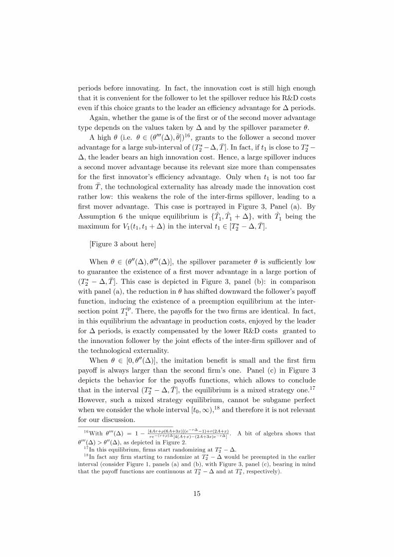
periods before innovating. In fact, the innovation cost is still high enoughthat it is convenient for the follower to let the spillover reduce his R&D costseven if this choice grants to the leader an e¢ ciency advantage for � periods.

Again, whether the game is of the �rst or of the second mover advantagetype depends on the values taken by � and by the spillover parameter �:

A high � (i.e. � 2 (�000(�); ��])16, grants to the follower a second moveradvantage for a large sub-interval of (T �2 ��; �T ]: In fact, if t1 is close to T �2 ��; the leader bears an high innovation cost. Hence, a large spillover inducesa second mover advantage because its relevant size more than compensatesfor the �rst innovator�s e¢ ciency advantage. Only when t1 is not too farfrom �T , the technological externality has already made the innovation costrather low: this weakens the role of the inter-�rms spillover, leading to a�rst mover advantage. This case is portrayed in Figure 3, Panel (a). ByAssumption 6 the unique equilibrium is fT̂1; T̂1 + �g; with T̂1 being themaximum for V1(t1; t1 +�) in the interval t1 2 [T �2 ��; �T ]:


When � 2 (�00(�); �000(�)]; the spillover parameter � is su¢ ciently lowto guarantee the existence of a �rst mover advantage in a large portion of(T �2 � �; �T ]: This case is depicted in Figure 3, panel (b): in comparisonwith panel (a), the reduction in � has shifted downward the follower�s payo¤function, inducing the existence of a preemption equilibrium at the inter-section point T ip1 : There, the payo¤s for the two �rms are identical. In fact,in this equilibrium the advantage in production costs, enjoyed by the leaderfor � periods; is exactly compensated by the lower R&D costs granted tothe innovation follower by the joint e¤ects of the inter-�rm spillover and ofthe technological externality.

When � 2 [0; �00(�)]; the imitation bene�t is small and the �rst �rmpayo¤ is always larger than the second �rm�s one. Panel (c) in Figure 3depicts the behavior for the payo¤s functions, which allows to concludethat in the interval (T �2 ��; �T ]; the equilibrium is a mixed strategy one.17

However, such a mixed strategy equilibrium, cannot be subgame perfectwhen we consider the whole interval [t0;1);18 and therefore it is not relevantfor our discussion.

16With �000(�) = 1 � [4Ar+�(6A+3x)](e�r��1)+r(2A+x)re�(r+�)�[4(A+x)�(2A+3x)e�r�] . A bit of algebra shows that

�000(�) > �00(�); as depicted in Figure 2.17 In this equilibrium, �rms start randomizing at T �2 ��:18 In fact any �rm starting to randomize at T �2 �� would be preempted in the earlier

interval (consider Figure 1, panels (a) and (b), with Figure 3, panel (c), bearing in mindthat the payo¤ functions are continuous at T �2 �� and at T �2 ; respectively).

15

The above arguments are summarized in:

Proposition 2

Let �T = t0 � 1� ln

�4A(1�e�r�)

9br [1�(1��)e�(r+�)�]

�:

When Assumptions 2, 3 and 4 are satis�ed, in the interval t1 2 (T �2 ��; �T ];

(a) if � 2 (�000(�); ��]; the unique subgame perfect equilibrium is fT̂1; T̂1+�g; where:

T̂1 = t0 �1

�ln

�4(A+ x)� (2A+ 3x)e�r�

9b (r + �)

�;

(b) if � 2 [�00(�); �000(�)] the unique subgame perfect equilibrium isfT ip1 ; T

ip1 +�g; where:

T ip1 = t0 �1

�ln

�3(2A+ x)(1� e�r�)

9br [1� (1� �)e�(r+�)�]

�: (13)

(c) if � 2 [0; �00(�)); there is no pure strategy equilibrium in the interval[T �2 ��; �T ]:


�T is raised by an increase in the inter-�rm spillover: in fact, a morerelevant bene�t from imitation postpones the undertaking of a line of actionthat prescribes the forsaking of the bene�t itself.19

More interestingly, we see from (13) that in case (b) an increase in theinter-�rm spillover delays the equilibrium. This happens because the equi-librium fT ip1 ; T

ip1 + �g is preemptive: the �rst innovator sinks the R&D

costs as soon as her payo¤s becomes larger than the rival�s one. Because anhigher � bene�ts the follower, it also softens the incentive to invest for theleader and hence mitigates the competitive pressure.

We conclude this Sub-section by jointly discussing the results obtainedin Propositions 1 and 2, which allow us to select the equilibrium in the wholeinterval [t0; �T ] for most parameters con�gurations.

When � 2 (maxf�0(�); �00(�)g; ��]; which is in area C of Figure 2, theintermediate equilibrium is the one described in Proposition 2, parts (a)and (b)), while, in the interval [t0; T �2 ��]; the equilibrium is fT �2 ��; T �2 g(Proposition 1, part (c)). Since V1(t1; t1 + �) is increasing in the whole

19Apart from the e¤ect of �; the comparative static for �T is quite similar to the one forT �2 :

16

interval t1 2 (t0; T �2 ��] (Figure 1, panel (c)); the intermediate equilibriumis the subgame perfect one in the interval [t0; �T ]: there is no �rst �rmdeviation payo¤ that can undermine this equilibrium for t1 2 [t0; �T ]:

When � 2 [0; �00(�)] (i.e. in the lower portion of area A and in area B ofFigure 2), the intermediate equilibrium is not relevant: any �rm investing in[T �2 ��; �T ] would be preempted in the earlier interval. (Bear in mind thatthe two payo¤ functions are continuous at T �2 �� and at T �2 ; respectively,and consider Figure 1, panels (a) and (b), and Figure 3, panel (c)). Accord-ingly, the pure strategy preemption equilibrium which exists in [t0; T �2 ��]�as granted by Proposition 1, parts (a) and (b) � is the subgame perfectequilibrium in [t0; �T ]:

In the remainder of area A and in area D (i.e. for �00(�) < � < �0(�)),the �rst innovator payo¤ function has local maxima both in (t0; T �2 ��] andin (T �2 � �; �T ] (Proposition 1, parts (a) and (d) and Proposition 2, parts(a). Refer also to panels (a) and (b) in Figure 1 and to panel (a) in Figure3). In this case, the equilibrium selection on the ground of the subgameperfectness criterion requires the use of numerical simulations. This analysiswill be carried out in Sub-section 3.3.

3.2.3 The late equilibrium

Finally, if the innovation leader decides to invest �late� (i.e. when t1 2[ �T ;1)) the R&D cost is so low that it is optimal for the second �rm toimmediately enter upon rival�s investment, without exploiting the inter-�rmspillover.

In this case the �rst �rm is aware that�as soon as she innovates�thesecond �rm will �immediately�follow her decision, and invest. Hence, each�rm takes her decision anticipating such a follower�s behavior. This leadsto an equilibrium where the two �rms maximize their joint payo¤: knowingthat it will be immediately followed, each �rm delays its innovation until itsdiscounted sum of pro�ts reaches its maximum. In this context, where �rmsremain symmetric, the maximization of a single �rm�s payo¤ coincides withtheir joint maximization.

Formally, the innovation leader�s behavior is summarized by the followingproposition.

Proposition 3

When Assumptions 2, 3 and 4 are satis�ed, for t1 2 [ �T ;1);(a) if � 2 [�̂(�); ��] where �̂(�) = 1 � e(r+�)�

h1� (r + �)1�e�r�r

4A2A+x

i;

both �rms invest at �T ;

17

(b) if � 2 [1� r+�r e

�� + �r e(r+�)�; �̂(�)); both �rms invest at:

T le = t0 �1

�ln

�2A+ x

9b (r + �)

�: (14)

(c) if � 2 [0; 1 � r+�r e

�� + �r e(r+�)�); the subgame perfect equilibrium

is either T le; or it is such that it cannot be subgame perfect in the intervalt1 2 [t0;1).


When the spillover is low, the scope for waiting � before investing islimited and hence �T is low. Therefore, for a low � the payo¤-maximizingchoice for the adoption time is unconstrained and thus the late equilibriumis given by (14).

3.3 Equilibrium selection

As already remarked, subgame perfectness is the criterion we use to se-lect among the equilibria identi�ed in the previous Sub-section. Subgameperfectness requires that the equilibrium must survive all the possible o¤-equilibrium deviations. Accordingly, in the present context, the equilibriumselection must be carried out comparing the leader�s payo¤ at any candidateequilibrium, with her payo¤ at any adoption date earlier than the one thatis part of the equilibrium. Unfortunately, this task cannot be performedanalytically, due to the high degree of non linearity in our model. Hence,we now present some numerical results.20

In our simulations, we normalize to unity the market dimension para-meter A, and we �x the discount rate r to 0.03, which is consistent withcomputing calendar time in years. The parameter does not play any sub-stantial role: the e¤ect of an higher (i.e. of a less e¢ cient R&D) is topostpone all of the equilibria, without changing their relative convenience.Likewise, the choice for b is inconsequential: an increase in b always inducesa proportional contraction in per period pro�ts. Hence, we choose b = 1

and = 150 with no loss of generality. As for �; we study�in the schum-peterian tradition�industry-speci�c rates of reduction in innovation costs.Industry I is technologically mature, but it still bene�ts from some technicalprogress in the sectors producing its machinery. Accordingly, � = 0:01: In

20Our routine has been written in Gauss, and it is based on a discretization of thespace [� x �]; for � 2 [10(�10); 0:8] and � 2 [10(�10); 3]: We have used 240.000 gridpoints,however our results do not relevantly change for any number of evaluation points largerthan 15.000. This routine is available upon request from the authors.

18

industry II, � = 0:05; which is the case of a fairly dynamic sector. Finally,industry III is a sector involved in a �technical revolution�, where � = 0:09.To appreciate our �gures, consider that the average economy-wide increasein productivity is of the order of 2% a year; moreover consider that thecost-e¤ective technical progress parameter, �; may well be lower than theproductivity growth rate, due to increases in the real wage in the researchsectors.

To preserve the duopolistic structure of our market, we consider onlynon-drastic innovation (Assumption 1). Hence, the size of the R&D output,x; is lower than A (x < 1): We investigate two types of innovative output:a moderate innovation where x = 0:05A(= 0:05) and a major innovationwhere x = 0:5A(= 0:5):

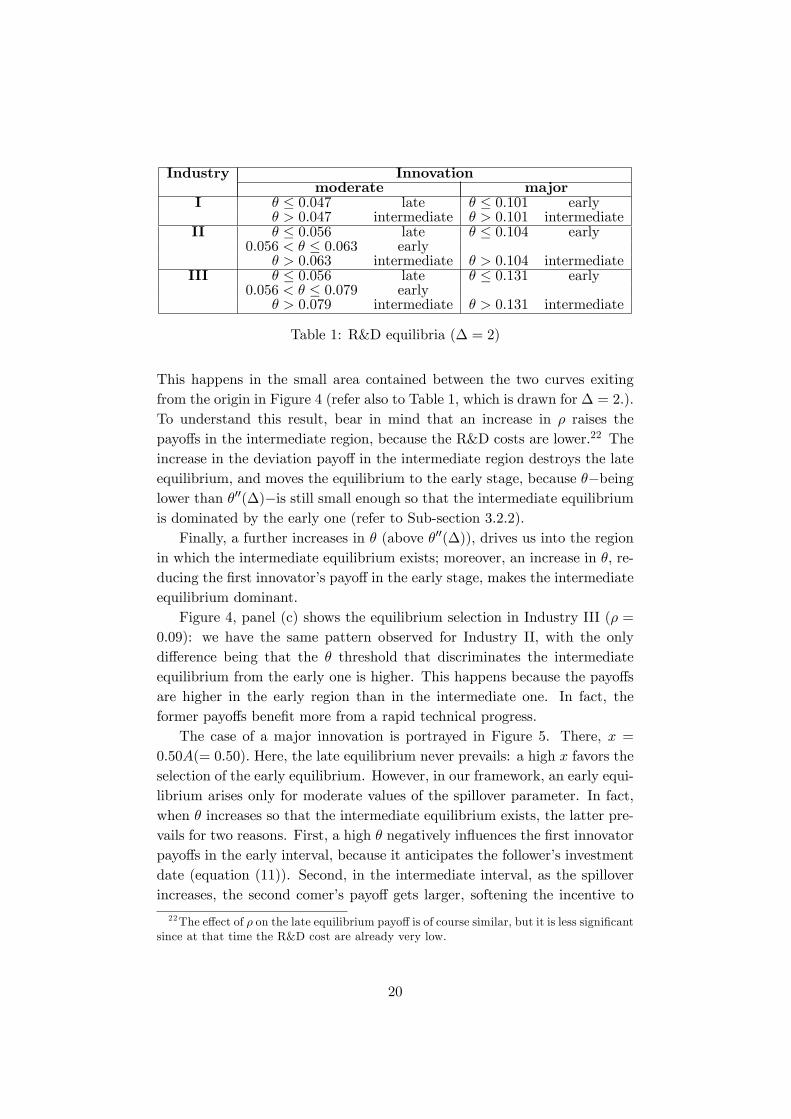
Figure 4 portrays the equilibria arising in the case of a moderate inno-vation. Panel (a) highlights that in Industry I a low spillover implies, for agiven �; a late equilibrium, while as the spillover increases the intermedi-ate equilibrium prevails. For instance, when � = 2; (refer to Table 1) thelate equilibrium prevails when � � 0:047, while if � > 0:047 we have theintermediate equilibrium.


The intuition for this result is the following: as underscored by Fuden-berg and Tirole (1985), the smaller the cost reduction, the weaker is theincentive to innovate �rst.21 Hence, a small x means that the highest de-viation payo¤ for an early innovator is low, so that the early equilibriumnever prevails over the late one. Moreover, a low spillover gives rise to alate equilibrium because it shrinks the intermediate region, since the second�rm has a weak incentive to wait � to enjoy a modest R&D cost-reducingspillover (refer to the de�nition for �T and to Figure 3, panel (c)). Hence,the late equilibrium prevails over any possible deviation occurring in theintermediate period.

When � grows, the intermediate region enlarges, leading to a situationin which the �rst �rm�s deviation payo¤ becomes greater than her late equi-librium payo¤. This leads to the prevalence of the intermediate equilibrium.

Panel (b) in Figure 4 shows the equilibria arising in Industry II. Again,for a given �; if the spillover is very low, the equilibrium in the R&D stageis the late one, for the same reasons as explained before. However, as �increases (but it is still lower than �00(�)), the early equilibrium prevails.

21This happens because the single innovator pro�t function, �101 ; is more convex in xthan �111 (see Sub-section 2.1).

19

Industry Innovationmoderate major

I � � 0:047 late � � 0:101 early� > 0:047 intermediate � > 0:101 intermediate

II � � 0:056 late � � 0:104 early0:056 < � � 0:063 early

� > 0:063 intermediate � > 0:104 intermediateIII � � 0:056 late � � 0:131 early

0:056 < � � 0:079 early� > 0:079 intermediate � > 0:131 intermediate

Table 1: R&D equilibria (� = 2)

This happens in the small area contained between the two curves exitingfrom the origin in Figure 4 (refer also to Table 1, which is drawn for � = 2:).To understand this result, bear in mind that an increase in � raises thepayo¤s in the intermediate region, because the R&D costs are lower.22 Theincrease in the deviation payo¤ in the intermediate region destroys the lateequilibrium, and moves the equilibrium to the early stage, because ��beinglower than �00(�)�is still small enough so that the intermediate equilibriumis dominated by the early one (refer to Sub-section 3.2.2).

Finally, a further increases in � (above �00(�)), drives us into the regionin which the intermediate equilibrium exists; moreover, an increase in �; re-ducing the �rst innovator�s payo¤ in the early stage, makes the intermediateequilibrium dominant.

Figure 4, panel (c) shows the equilibrium selection in Industry III (� =0:09): we have the same pattern observed for Industry II, with the onlydi¤erence being that the � threshold that discriminates the intermediateequilibrium from the early one is higher. This happens because the payo¤sare higher in the early region than in the intermediate one. In fact, theformer payo¤s bene�t more from a rapid technical progress.

The case of a major innovation is portrayed in Figure 5. There, x =0:50A(= 0:50): Here, the late equilibrium never prevails: a high x favors theselection of the early equilibrium. However, in our framework, an early equi-librium arises only for moderate values of the spillover parameter. In fact,when � increases so that the intermediate equilibrium exists, the latter pre-vails for two reasons. First, a high � negatively in�uences the �rst innovatorpayo¤s in the early interval, because it anticipates the follower�s investmentdate (equation (11)). Second, in the intermediate interval, as the spilloverincreases, the second comer�s payo¤ gets larger, softening the incentive to

22The e¤ect of � on the late equilibrium payo¤ is of course similar, but it is less signi�cantsince at that time the R&D cost are already very low.

20

invest for the leader. This milder competition implies higher payo¤s for both�rms, inducing the selection of the intermediate equilibrium.


In sum, our analysis of the equilibrium selection process suggests thatthe intermediate equilibrium is the subgame perfect one in large portions ofthe parameter space.

This may help to explain the results in Schmidt-Dengler (2006). He esti-mates the determinants of the adoption of equipment for magnetic resolutionimages, which allows him to disentangle the preemption from the stand alonepro�t-maximizing e¤ect. He �nds that preemption accounts only for a rela-tively small share of the acceleration of investment timing that caracterizesthe duopolistic market solution when compared to the collusive scenario.This is what our model prescribes for � > �00(�).

4 Welfare analysis

Having characterized the market equilibria, we can now analyze the benev-olent planner problem.

In dealing with this issue, we introduce some hypotheses. First, weadopt a second best perspective, assuming that neither the number of �rmsacting in the market nor the way they compete in the second stage quantitygame lies within the regulatory power of the benevolent planner. Hence,what this non-omnipotent planner can choose, is the timing of innovation.23

Therefore, its decisions will be based on the instantaneous welfare levels �computed in Sub-section 2.1 �that have been obtained under the Cournotdecentralized solution.

Second, the spillover obtained by �rms engaging in a joint R&D projectat the dates induced by the planner, is the same that is grasped by thesecond entrant when he waits � (i.e., the joint R&D activity grants a fasterinformation �ow, but not a cost advantage, when compared to a decentral-ized solution). The innovation costs incorporate the expenditures for thetraining of the employees required by the new production process, for somenew machineries (or for adaptation of the existing plant), and so on (see De

23This approach is standard in the literature: see Stenbacka and Tombak (1994), Hoppe(2000), and Weeds (2002). The �rst best equilibrium for an omnipotent planner impliesthe presence of only one �rm: whenever there are non-decreasing returns in the innovationsize or probability, it is optimal to have only one �rm to innovate and cover the entiremarket at the marginal (post-innovation) cost.

21

Bondt (1996)). Hence, the spillover parameter is not signi�cantly increasedby an R&D agreement.24

Therefore, the social planner maximizes �with respect to the adoptiondates t1 and t2 �the following welfare function

W1(t1; t2) =

Z t1

t0

W 00e�r(t�t0)dt+

Z t2

t1

W 10e�r(t�t0)dt+

Z 1

t2

W 111 e

�r(t�t0)dt

� xe�(r+�)(t1�t0) � (1� �) xe�(r+�)(t2�t0); (15)

where the (second best) instantaneous welfare levels, are given by Eqs. (2),(4) and (6), and t1 � t2 is a natural constraint.

The maximization of (15) yields

TSP1 = t0 �1

�ln

�8A+ 11x

18b (r + �)

�; TSP2 = t0 �

1

�ln

�8A� 3x

18b (r + �)(1� �)

�;

if � � 14x8A+11x ; and

TSP1 = TSP2 = TSP = t0 �1

�ln

�8A+ 4x

9b (r + �)(2� �)

�;

if not. The superscript SP stands for �social planner�.To verify whether the decentralized solution induces overinvestment in

comparison with the centralized one, we compare the discounted (to t0) in-novation costs implied by the subgame perfect market solution with thoseobtained by the social planner. When the market innovation costs are higher(lower) than the planner solution ones, there is overinvestment (underivest-ment). The di¤erence in the �rms�timings that characterize the centralizedsolution and the decentralized one adds to the ine¢ ciency related to the useof a non-optimal amount of resources.

Because the market game often does not have a closed form solution,to appreciate the di¤erences in the discounted innovation costs, we need torely on numerical simulations, which allow to obtain the following results:

i) Whenever the early equilibrium prevails, the market solution implies anexcessive use of resources (i.e. overinvestment).

ii) Symmetrically, when the late equilibrium is subgame perfect, the decen-tralized solution involves a too low level of investment.

24The alternative assumption of an increasing � will be brie�y discussed in footnote 26.

22

iii) When the intermediate equilibrium dominates, it implies underinvest-ment, but for a small parameters sub-set when the size of the inno-vation is small, and the speed of the exogenous technical progress ishigh.

While the �rst two results are intuitive, the third deserves more atten-tion.

To understand why an overinvesting intermediate equilibrium is possibleonly if the innovation size is small, consider the analysis in Sub-section 2.1.There, we have shown that both the instantaneous social welfare, and the�rms pro�ts increase more than proportionally with the size of the innova-tion. Because the social welfare is larger than the �rms pro�t, also the wedgebetween the social and the private incentives to innovate increases with x;which acts against the possibility of overinvestment with a large innovation.

An increase in � reduces both the social planner�s optimal adoptiondate(s) and the intermediate equilibrium ones. In the market game a steepercost reduction pro�le, has strong e¤ects on the innovation dates. In fact,given the leader�s optimal timing, a faster cost reduction bene�ts the fol-lower�s payo¤. This provides an incentive for his preemptive behavior, whichmay lead to overinvestment.

Accordingly, the portion of the parameter space with overinvestment isthe widest, the largest is �, and the lowest is x. However, even in this case,the overinvestment area is very small: e. g. for � = 0:09; x = 0:05, and � =2, the intermediate equilibrium implies overivestment for � 2 [0:080; 0:115]:25

Hence, not only the intermediate equilibrium prevails for most of the pa-rameter con�gurations (as shown in Sub-section 3.3), but it also implies thatthe duopolistic market equilibrium involves underinvestment. This applieseven when the innovation size is large, and hence the incentives to hasteninnovation are remarkable. Therefore, the market equilibrium calls for pub-lic policies aimed at increasing the research activity even in this case, unlessthe inter-�rm spillover is very low. Notice that the natural indicators ofa highly competitive environment, namely a di¤usion equilibrium and rentequalization, do not necessarily imply that the R&D investment is excessivefrom the social planner�s perspective.

When we focus on minor innovations � the case in which the marketequilibrium underinvests, according to the earlier literature �our result im-ply that the policies aimed at stimulating R&D have to be less sizeablethan suggested before, because the underinvesting intermediate equilibrium

25Notice that Assumption 6 applies only if � > �000(�), i.e. when the intermediateequilibrium already implies underinvestment. Hence, it is not crucial for our results.

23

is closer to the social optimum than the late equilibrium.26

5 Conclusions

In our duopoly game, �rms, in addition to a technological externality, takesinto account a spillover that lowers the second comer�s innovation cost. Thisspillover exerts its e¤ect after a �disclosure lag�. In this setting, a newequilibrium arises, in which the R&D investment takes place at intermediatedates in comparison with those already identi�ed in the literature.

Preemption, R&D di¤usion, and the possibility of rent equalization char-acterize the intermediate equilibrium, which is competitive, although in amild form. The intermediate equilibrium is subgame perfect for a large rangeof the parameters set; moreover, it is socially ine¢ cient, implying a low levelof investment in R&D.

This happens even in presence of major innovations, despite the largeincentive to invest in R&D provided by this type of innovation. This re-sult has important implications for innovation policy. For example, researchjoint ventures should be assessed in more favorable terms than those im-plied by the literature following d�Aspremont and Jacquemin (1988), andKamien, Muller, and Zhang (1992). In fact, while a RJV may underinvestin comparison to an highly competitive equilibrium, it is likely to improvesocial welfare over a �mildly competitive�, underinvesting, market outcome.Furthermore, our paper suggests that R&D subsidies should be set in placein a range of market con�gurations wider than that has been previously pro-posed. Finally, our analysis provides an argument against the use of entryregulations (or price caps), which are sometimes used to slow technologyadoption, e.g. in telecommunication industries. We leave the analysis ofthese policy instruments for further research.

When the innovation size is small, the prevalence of the intermediateequilibrium implies that R&D enhancing policies must be less intense thandevised in the earlier literature. Actually, policies designed without takinginto account the inter-�rm spillover can be largely oversized, even whenthe spillover is quantitatively modest. Notice also that the intermediateequilibrium calls for moderate policies, which may prove easy to implement

26Suppose that a joint R&D activity guarantees not only a faster but also an easier,and hence less costly, information �ow. In this case the spillover parameter in Eq. (15)should be higher than in the market game, and the social planner should dictate earlierinvestment date(s). Under this alternative assumption, result ii) is una¤ected, result iii)is strenghtened, because it applies for even larger parameters set, while result i) weakens.In fact, it is possible � for a sizeable (and somehow irrealistic) increase in � � that thesecond best optimal timing anticipates the early equilibrium ones.

24

from a political economy perspective.Our setting can be extended in various directions, which however, would

require an heavy use of numerical techniques. For example, it would be inter-esting to consider a stochastic inter-�rm spillover, in which the probabilityof information di¤usion depends upon the time elapsed from the introduc-tion of the innovation, and on the follower�s imitation e¤ort. Also, we wouldlike to consider the possibility that the leader actively (and hence costly)attempts to prevent information leakages, thereby increasing the disclosurelag. Whenever the �rms�e¤orts lenghten this lag, they reduce the follower�sequilibrium payo¤, and hence, also the leader�s one. Therefore, they tend toreduce the intermediate equilibrium dominance area. However, the analy-sis developed in Section 3.3 suggests that the e¤ect of the disclosure lagon the dominance areas are weak. Hence, our main result should not beundermined by the adoption of a richer framework.

References

Beath, J., Katsoulacos, Y. and Ulph, D. �Strategic R&D Policy�, EconomicJournal, Vol. 99 (1989), pp. 74-83.

Cohen, W.M., Goto A., Nagata A., Nelson R.R., andWalsh, J.P., �R&D spillovers,patents and the incentives to innovate in Japan and the United States�, Re-search Policy, Vol. 31 (2002), pp. 1349-1367.

Dasgupta, P., �Patents, priority and imitation or, the economics of races andwaiting games.�Economic Journal, Vol. 98 (1988), pp. 66�80.

d�Aspremont, C., and Jacquemin, A., �Cooperative and Non-cooperative R&Din Duopoly with Spillovers.�American Economic Review, Vol. 78 (1988),pp. 1133�1137.

De Bondt, R., �Spillovers and innovative activities.� International Journal ofIndustrial Organization, Vol. 15 (1996), pp. 1�28.

Delbono, F. and Denicolò, V. �Incentives to innovate in a Cournot oligopoly.�Quarterly Journal of Economics, Vol. 105 (1991), pp.950-961.

Denicolò, V., �Patent Races and Optimal Patent Breadth and Length.�Journalof Industrial Economics, Vol. 44 (1996), pp. 249�265.

Dutta, P. K., Lach, S., and Rustichini, A., �Better Late Than Early: VerticalDi¤erentiation in the Adoption of a New Technology �Journal of Economicsand Management Strategy, Vol. 4 (1995), pp. 563-89.

25

Fudenberg, D., and Tirole, J., �Preemption and Rent Equalization in the Adop-tion of New Technology.�Review of Economic Studies, Vol. 52 (1985), pp.383�401.

� Game Theory. Cambridge, MA: MIT Press, 1991.Hernan, R., Marin, P.L., and Siotis, G., �An Empirical Evaluation of the Deter-

minants of Research Joint Venture Formation.�Journal of Industrial Eco-nomics, Vol. 51 (2003), pp. 75�89.

Hoppe, H.C., �Second-mover advantages in the strategic adoption of new tech-nology under uncertainty.�International Journal of Industrial Organization,Vol. 18 (2000), pp. 315�338.

Hoppe, H.C., �The timing of new technology adoption: theoretical models andempirical evidence.�The Manchester School, Vol. 70 (2002), pp. 56-76.

Hoppe, H.C., Lehmann-Grube, U., �Innovation Timing Games: A General Frame-work with Applications.�Journal of Economic Theory, Vol. 121 (2005), pp.30�50.

Jin, J.Y., and Troege, M., �R&D Competition and Endogenous Spillovers.�TheManchester School, Vol. 74 (2006), pp. 40�51.

Kamien, M.I., Muller, E., and Zhang, I., �Research Joint Ventures and R&DCartels.�American Economic Review, Vol. 82 (1992), pp. 1293�1306.

Katz, M.L., and Shapiro, C., �R&D Rivalry with Licensing or Imitation.�Amer-ican Economic Review, Vol. 77 (1987), pp. 402�420.

Lee, T. and Wilde, L., �Market structure and innovation: a reformulation.�Quarterly Journal of Economics, Vol. 94 (1980), pp.429-36.

Loury, G., �Market structure and innovation.�Quarterly Journal of Economics,Vol. 93 (1979), pp.395-410.

Mans�eld, E., �How Rapidly Does New Industrial Technology Leak Out?�Jour-nal of Industrial Economics, Vol. 34 (1985), pp. 217�223.

Mans�eld, E., Schwartz, M., and Wagner, S., �Imitation Costs and Patents: AnEmpirical Study.�Economic Journal, Vol. 91 (1981), pp. 907�918.

Reinganum, J., �On the di¤usion of new technologies: a game theoretic ap-proach.�Review of Economic Studies, Vol. 48, pp. 395-405.

Riordan, M.H., �Regulation and preemptive technology adoption.�RAND Jour-nal of Economics Vol. 23 (1992), pp.334-349.

Schmidt-Dengler, P., �The Timing of New Technology Adoption: The Case ofMRI�, mimeo LSE ; (2006).

Stenbacka, R. and Tombak, M.H., �Strategic timing of adoption of new technolo-gies under uncertainty.� International Journal of Industrial Organization,Vol. 12 (1994), pp. 387�411.

Weeds, H., �Strategic Delay in a Real Options Model of R&D Competition.�Review of Economic Studies, Vol. 69 (2002), pp. 729�747.

26

APPENDIX

Proof of Proposition 1As a preliminary, notice that Assumption 4 guarantees that the interval [t0; T �2 �

�] is non empty for � 2 [0; ��]: Notice, moreover, that Assumption 2 impliesthat all the four sub-cases in Proposition 1 are well de�ned. This is becauseAssumption 2 can be written as: �� max

nx

A+x ; �00( ��)

o:

Proof of part (a). As it is standard, we start characterizing the optimal strategyfor the follower. When the �rst �rm has sunk the innovation cost at timet1 2 [t0; T �2 ��], the payo¤ at time t0 for the second �rm, when it investsat t2; is given by (10).

Suppose that the second comer decides to wait more than �; to grasp the inter-�rms spillover; in this case Eq. (8) prescribes that the innovation cost isC2(T2) = (1 � �) xe��(T2�t0); and a few straightforward calculations showthat T �2 ; as given by (11), maximizes V2(t1; t2):

Alternatively, the second comer could decide not to wait for � periods, and inthis case he should invest at:

T 02 = t0 �1

�ln

�4A

9b (r + �)

�: (A.1)

This second alternative requires that T 02 2 [t1; t1+�). Had the latter restrictionnot been satis�ed, the innovation follower would have bene�ted from thespillover. Since T 02 > T

�2 , whenever t1 2 [t0; T �2 ��] the innovation follower

grasps the imitation bene�ts and invests at T �2 : Because of this, his payo¤can be written as:

V2(t1; T�2 ) =

A2

9br��(2A� x)x9br

�e�r(t1�t0)

+�

r(r + �)

4Ax

9b

�4A

9b (r + �)(1� �)

� r�

; (A.2)

which implies: @V2(t1;T �2 )@t1

> 0; and @2V2(t1;T �2 )(@t1)2

< 0 in the whole interval

[t0; T�2 ��]. Also notice that

@V2(t1;T �2 )@� > 0 for every t1 2 [t0; T �2 ��]:

Having determined the optimal decision for the follower, we now determine theleader�s best strategy. When t1 2 [t0; T �2 ��]; the innovation leader payo¤ isgiven by (9) in which the innovation costs are provided by (7) and t2 = T �2 :

Exploiting equation (11), we obtain:

27

V1(t1; T�2 ) =

A2

9br+

�4(A+ x)x

9br� xe��(t1�t0)

�e�r(t1�t0)

�(2A+ 3x)x9br

�4A

9b (r + �)(1� �)

� r�

: (A.3)

Hence, @V1(t1;T�2 )

@t1? 0 when t1 7 T �1 (with T �1 given by (12)). Notice that T �1 , in

general, need not be smaller than T �2 � �: Notice also that@V1(t1;T �2 )

@� < 0

for every t1 2 [t0; T �2 ��]:When � � �0(�); it is easy to show that T �1 � T �2 � �; because the latter

inequality requires A + x � A1��e

��; and hence � � 1 � AA+xe

��: We nowcheck whether � when t1 = T �1� the leader�s payo¤ is larger than thefollower�s one. Exploiting equation (A.3), V1(T �1 ; T

�2 ) can be easily written

as:

V1(T�1 ; T

�2 ) =

=A2

9br+4�(A+ x)x

9br(r + �)

�4(A+ x)

9b (r + �)

� r�

� (2A+ 3x)x9br

�4A

9b (r + �)(1� �)

� r�

;

while, from (A.2), V2(T �1 ; T�2 ) is:

V2(T�1 ; T

�2 ) =

=A2

9br� (2A� x)x

9br

�4(A+ x)

9b (r + �)

� r�

+�

r(r + �)

4Ax

9b

�4A

9b (r + �)(1� �)

� r�

:

A few calculations allow us to show that V1(T �1 ; T�2 ) � V2(T �1 ; T �2 ) if � � ~�: Notice

moreover that ~� � �0(�) for � 2 [0;�0]; where

�0 =1

rln

�1 +

r4x

�3(2A+ x) + r(2A� x)

�> 0:

Hence, V1(T �1 ; T�2 ) � V2(T

�1 ; T

�2 ) and T

�1 < T �2 � � if � � minf~�; �0(�)g:

Because �0 > 0; and �0(�) > 0; we have that ~� > 0; which guarantees thatthe region � � minf~�; �0(�)g is non-empty.

To conclude that the �rst �rm equilibrium adoption date ismaxfT¯ 1;t0g; we follow

the argument developed in Fudenberg and Tirole (1985): when V1(T �1 ; T�2 ) >

V2(T�1 ; T

�2 ); it is in each �rm�s interest to adopt at time T

�1 if the other �rm

has not adopted up to that time. But if a �rm knows that the other willadopt at time T �1 , it is in its interest to preempt at time T

�1 � dt, whenever

V1(T�1 � dt; T �2 ) � V2(T �1 ; T �2 ): By backward induction, we conclude that the

28

equilibrium strategy for the �rst innovator is maxfT¯ 1;t0g; where T¯ 1 is the

earliest adoption date such that V1(T¯ 1; T �2 ) � V2(T¯ 1

; T �2 ): In this case no�rm wants to invest and anticipate the other to avoid be preempted lateron. Mixed strategy equilibria are ruled out by Assumption 4. Hence, Part(a) is proved.

We now consider case (b), i.e. �0(�) < � � �00(�): A few calculations show thatthe restriction � � �00(�); implies: V1(T �2 ��; T �2 ) � V2(T �2 ��; T �2 ): Hence,the preemption argument sketched above applies again and the equilibriumis {maxfT

¯ 1;t0g; T �2 g (refer to Figure 1, panel (b)): Notice that, at � = �0;

�0(�0) = �00(�0)(= ~�): Therefore, this case applies only when � � �0: Thiscompletes the proof of Part (b).

To prove Part (c), split the restriction � > maxf�0(�); �00(�)g; into � > �0(�);and � > �00(�) (which must hold simultaneously). The restriction � > �0(�)implies that T �1 > T

�2 �� and hence that V1(t1; T �2 ) is increasing in the whole

interval t1 2 [t0; T �2 ��]: In its turn, � > �00(�) implies V2(T �2 ��; T �2 ) >V1(T

�2 ��; T �2 ): Hence, it is in each �rm�s interest to wait until T �2 ��; while

the preemption argument does not apply. By Assumption 6, this completesthe proof of Part (c).

Finally, we analyze case (d), i.e. ~� < � � �0(�): The restriction � � �0(�)

implies T �1 � T �2 ��: However, if � > ~�, as shown in Part (a), V1(T �1 ; T �2 ) <V2(T

�1 ; T

�2 ). Therefore, by Assumption 6, the �rst �rm becomes the leader

and invest at T �1 , while the second invests at T�2 : This completes the proof

of Part (d).

Proof of Proposition 2As a preliminary, notice that Assumption 2 guarantees that all the sub-cases in

Proposition 2 are well de�ned.Notice, moreover, that �T > T �2 �� for any � 2 [0; ��]:Notice, �nally, that some tedious calculations grant that: �000(�) � �00(�):As before, we start characterizing the optimal strategy for the follower.When t1 � T �2 ��; the innovation follower will never wait more than �, simply

because t1 � T �2 ��: Hence, his available strategies are:(1) wait exactly � periods to grasp the bene�t of the spillover,(2) invest immediately after the innovation leader, and(3) wait for a time span shorter than � (to exploit the exogenous technological

externality), and then invest (therefore, without exploiting the inter-�rmspillover).

First we compare what the innovation follower obtains by waiting � periods(strategy 1) with what he gets by investing immediately after the innovationleader (strategy 2). Hence, we determine when V2(t1; t1 + �) � V2(t1; t1):

29

This inequality immediately boils down to:

4Ax

9bre�r(t1+��t0) � (1� �) xe�(r+�)(t1+��t0)

� 4Ax

9bre�r(t1�t0) � xe�(r+�)(t1�t0);

which, in its turn, is satis�ed when: t1 � �T : Hence, the innovation followernever chooses to immediately follow the leader for any t1 2 [T �2 ��; �T ]:

Next, we compare strategy 1 with strategy 3.In doing so, recall the de�nition of T 02 from (A.1), and distinguish the case �T � T 02

from the case �T < T 02: Notice that the inequality �T � T 02 is satis�ed when� � 1 � r+�

r e�� + �

r e(r+�)�; and some calculations allow us to verify that:

�00(�) � 1� r+�r e

�� + �r e(r+�)�:

Hence, in cases (a) and (b), �T � T 02.Suppose now that the leader invests at t1 2 [T �2 ��; T 02��]: In this interval, the

payo¤ function for a follower who does not exploit the inter-�rm spillover isalways increasing. In fact, this function is concave with a global maximumat t2 = T 02 8 t1(refer to the Proof for Proposition 1). Hence, it is optimalfor the follower to invest later than T 02 ��; which implies that the spilloveris actually exploited.

When t1 2 (T 02 � �; T 02]; the optimal strategy for the innovation follower mustbe determined by comparing what it gets by delaying its investment for �periods with what can be obtained by investing at T 02: Hence, we need todetermine when V2(t1; t1+�)� V2(t1; T 02) � 0: This inequality immediatelyboils down to:

4Ax

9br

he�r(t1+��t0) � e�r(T 02�t0)

i� x

h(1� �)e�(r+�)(t1+��t0) � e�(r+�)(T 02�t0)

i� 0: (A.4)

It is easy to show that the left hand side of (A.4) is non-increasing in t1 inthe whole interval (T 02 � �; T 02]: Evaluate equation (A.4) at t1 = T 02, and�exploiting equation (A.1)�substitute out T 02 when convenient, to obtain:

e�r(T02�t0) 4Ax

9br

"e�r� � 1� r(1� �)e

�(r+�)�

r + �+

r

r + �

#� 0;

which is ful�lled when � � 1 � r+�r e

�� + �r e(r+�)�: Hence, under this re-

striction, the follower�s strategy of waiting � periods is chosen for anyt1 2 (T 02 ��; T 02]:

Finally, strategy 3 can never be optimal for t1 2 (T 02;�T ] simply because the

30

payo¤ function for a follower who does not exploit the spillover is decreasingin t2 2 (t1; �T ] and thus there is no point in waiting when the leader hasalready invested; recall moreover that the immediate investment strategyhas already been proven to be dominated by a time � delay.

Hence, in cases (a) and (b) the follower�s optimal reply to the innovation leader�sdecision to invest is to wait exactly� periods to grasp the inter-�rm spilloverand then invest.

The analysis for case (c) must be splitted into two sub-cases.c1) When � 2 [1 � r+�

r e�� + �

r e(r+�)�; �00(�)); then �T � T 02 and the analysis

developed above applies.c2) When � 2 [0; 1� r+�

r e��+ �

r e(r+�)�); then �T < T 02: Notice, however, that it is

possible to prove that T 02�� < �T : In the time interval t1 2 [T �2 ��; T 02��]the optimal strategy is again to wait � and exploit the inter-�rm spillover,because the follower�s payo¤ function V2(t1; t2) is increasing in t2 2 [t1; T 02��]:

When t1 2 (T 02 ��; �T ]; the optimal strategy for the innovation follower must bedetermined by comparing what he gets by delaying his investment for � pe-riods with what can be obtained by investing at T 02: Unfortunately, it is notpossible to characterize analytically the sub-intervals in which the two al-ternative strategies prevail. Let us denote by �T1 the instant when V2(t1; t1+�) = V2(t1; T

02):

�T1 2 (T 02 � �; �T ] because: V2(t1; t1 + �) � V2(t1; T 02) isnon-increasing in t1; lim�!0 [V2(T 02 ��+ �; T 02 + �)� V2(T 02 ��+ �; T 02)] >0 and V2( �T ; �T + �) � V2( �T ; T 02) < 0, in fact, by de�nition V2( �T ; �T + �) =V2( �T ; �T ) and V2( �T ; �T ) < V2( �T ; T 02): Hence, for t1 2 (T 02 ��; �T1] strategy (1)is optimal, while for t1 2 ( �T1; T 02] the innovation follower decides to innovateat T 02 (strategy 3).

We conclude our characterization for the follower�s optimal strategy by notingthat V2(t1; t1 + �) is a concave function with its maximum at the right ofT �2 ��:

We now proceed to analyzing the �rst �rm�s behavior.If � 2 (�000(�); ��] (case a), the �rst innovator is aware of the fact that her com-

petitor will always invest with a delay of � periods. Hence, she computesher payo¤ for t1 2 [T �2 ��; �T ] which is:

V1(t1; t1 +�) =A2

9br+��

4(A+ x)x

9br� xe��(t1�t0)

�� (2A+ 3x)x

9bre�r�

�e�r(t1�t0):

Notice that � � �00(�) implies that V2(T �2 ��; T �2 ) � V1(T �2 ��; T �2 ); hence the

31

latter inequality applies also for � � �000(�); notice moreover that the payo¤function V1(t1; t1 +�) reaches its maximum at t1 = T̂1:

Consider now the equation: V1(t1; t1 +�) = V2(t1; t1 +�); which has a unique

solution: T ip1 = t0 � 1� ln

�3(2A+x)(1�e�r�)

9br [1�(1��)e�(r+�)�]

�: Notice that T ip1 > T̂1 if

� > �000(�); hence for � 2 (�000(�); ��]; T ip1 2 [T̂1; �T ]: (This happens becausethe inter-�rm spillover is very high, implying a high payo¤ for the second�rm). Because the V2(t1; t1 + �) curve lies above the V1(t1; t1 + �) curvefor t1 2 [T �2 ��; T̂1]; no �rm has an incentive to preempt its rival before T̂1:The �rst �rm, under Assumption 6, has no incentive to delay her adoptionbeyond T̂1; because V1(t1; t1 + �) is decreasing for t1 2 [T̂1; �T ]: Hence, inthe interval [T �2 ��; �T ]; the unique subgame perfect equilibrium is t1 = T̂1;t2 = T̂1 + �: The �rst panel in Figure 3 portrays the situation analyzedhere. This proves Part (a).

In case (b) (� 2 [�00(�); �000(�)]); the �rst innovator is aware, again, of the factthat her competitor will invest with a delay of � periods. In this case,however, T ip1 2 [T �2 � �; T̂1]: in fact, with respect to the previous case,the reduction in the spillover parameter shifts downward the follower�s pay-o¤ function (as depicted in Figure 3, panel (b)) and, for t1 2 [T

ip1 ;�T ] the

V2(t1; t1 + �) curve lies below the V1(t1; t1 + �) curve. Hence, t1 = Tip1 is

part of the unique pure strategy equilibrium, due to the usual preemptionargument. This proves Part (b).

When considering the follower�s optimal strategy in case (c), we must distinguishagain the two sub-cases: c1) � 2 [1 � r+�

r e�� + �

r e(r+�)�; �00(�)); and c2)

� 2 [0; 1� r+�r e

�� + �r e(r+�)�):

c1) When � 2 [1 � r+�r e

�� + �r e(r+�)�; �00(�)); the �rst innovator is aware of

the fact that her competitor will invest with a delay of � periods. In thiscase one can show that the unique solution for the equation V1(t1; t1+�) =V2(t1; t1 + �); lies outside the interval [T

�2 � �; �T ]: (i.e. T

ip1 < T �2 � �):

Because the follower�s payo¤ is lower than the �rst innovator�s one, in thewhole interval [T �2 ��; �T ]; and standard arguments imply the existence ofa mixed strategy equilibrium, in which �rms start to randomize at T �2 ��:This case is portrayed in panel (c) of Figure 3.

c2) When � 2 [0; 1� r+�r e

��+ �r e(r+�)�); the �rst �rm is aware that, if she chooses

t1 2 [T �2 ��; �T1]; the follower picks an innovation time characterized by adelay of span �; while if she chooses t1 2 [ �T1; �T ] the follower innovates attime T 02 > �T :

Suppose �rst that the follower innovates with a delay of �: In this case, becauseT ip1 < T �2 ��; it is obvious that V1(t1; t1 +�) > V2(t1; t1 +�) for any t1 2[T �2 ��; �T ] and hence, a fortiori, for any t1 2 [T �2 ��; �T1]: Suppose now that

32

the follower innovates at time T 02: In this case, again, V1(t1; T02) > V2(t1; T

02)

for t1 2 [T 02��; �T ] and hence, a fortiori, for any t1 2 [ �T1; �T ]: (To show this,consider that V1(T 02; T

02) = V2(T

02; T

02) and that @[V1(t1; T

02)�V2(t1; T 02)]=@t1 <

0:). Hence, in the whole interval [T �2 ��; �T ]; the follower�s payo¤ is lowerthan the �rst innovator�s one; again standard arguments imply the existenceof a mixed strategy equilibrium, in which �rms start to randomize at T �2 ��:This proves Part (c).

Proof of Proposition 3.Notice, as a preliminary, that Assumption 2 guarantees that all the sub-cases in

Proposition 3 are non-empty.As usual, we start characterizing the optimal strategy for the follower.The proof of Proposition 2 implies that the innovation follower will never wait

�; for any t1 � �T : Hence, his available strategies are:(1) invest immediately after the innovation leader, and(2) wait for a time span shorter than � (to exploit the exogenous technological

externality), and then invest without exploiting the inter-�rm spillover.The proof of Proposition 1 implies that �when the innovation follower decides to

wait �he invests at T 02; for any t1 2 (T 02��; T 02]. In fact, the payo¤ functionfor the follower, V2(t1; t2) has a maximum at T 02:

In the proof for Proposition 2, we showed that, for � 2 [1� r+�r e

��+ �r e(r+�)�; ��];

then �T � T 02. Hence, under this parameter restriction, the second innovatorinvests immediately after the innovation leader. In fact, it is never in thefollower�s interest to wait � periods, because t1 > �T ; while the follower�spayo¤ function is decreasing in t2 in the whole interval t1 2 [ �T ;1): Hence,the follower has no point in waiting.

In contrast, when � 2 [0; 1� r+�r e

��+ �r e(r+�)�); then T 02�� < �T < T 02 (as shown

in the proof for Proposition 2). Therefore, under this parameter restriction,the second innovator invests at T 02 when t1 2 [ �T ; T 02]; when t1 2 (T 02;1); theinnovation follower invests immediately after the innovation leader becauseits payo¤ function is decreasing in t2.

We now analyze the �rst �rm�s behavior.Suppose �rst, that � 2 [1� r+�

r e��+ �

r e(r+�)�; ��]; so that the �rst �rm knows that

�as soon as she innovates �the rival �rm immediately sinks the innovationcost.

Hence, the payo¤ for the �rst �rm is:

33

V1(t1; t1) =

Z t1

t0

�001 e�r(t�t0)dt+

+

Z 1

t1

�111 e�r(t�t0)dt� xe�(r+�)(t1�t0): (A.5)

Maximization of (A.5) with respect to t1 under the constraint t1 � �T yields thatthe �rst �rm optimal timing is:

�T if � � �̂(�);T le = t0 � 1

� ln�

2A+x9b (r+�)

�if � < �̂(�):

It is now easy to show that �̂(�) � 1 � r+�r e

�� + �r e(r+�)�: Accordingly, when

� � �̂(�); both �rms invest at �T : This proves part (a).To prove part (b), notice �rst that � when � 2 [1� r+�

r e��+ �

r e(r+�)�; �̂(�))� the

second �rm invests immediately after the �rst �rm. Hence, the equilibriumis T le:

Finally, consider part (c), which requires. � 2 [0; 1� r+�r e

�� + �r e(r+�)�): When

t1 2 [ �T ; T 02] the second �rm invests at T 02; when t1 2 [T 02;1); the second �rminvests immediately after the �rst one. For the �rst �rm, the optimal replyto T 02 would be to invest at �T : In fact,

@V1(t1;T 02)@t1

< 0 for t1 2 [ �T ; T 02] (di¤er-entiate V1(t1; T 02) and check that �T � T �1 ): Notice that, for t1 2 [ �T ; T 02) theinnovation leader�s payo¤ is higher than the follower�s one. (This is shownby noting that V1(T 02; T

02) = V2(T

02; T

02); and that

@V1(t1;T 02)@t1

� @V2(t1;T 02)@t1

fort1 2 [T 02 � �; T 02]; and therefore, a fortiori, for t1 2 [ �T ; T 02].) The �rstmover advantage interval t1 2 [ �T ; T 02] gives rise to preemptive behaviors ifV1( �T ; T

02) � V1(T le; T le): Hence, in the interval t1 2 [ �T ;1); the equilibrium

is T le when V1( �T ; T 02) < V1(Tle; T le). Instead, when V1( �T ; T 02) � V1(T le; T le);

we have a mixed strategy equilibrium, in which �rms randomize at �T : (How-ever, notice that the preemption argument implies that such an equilibriumis not subgame perfect for t1 2 [t0;1); in fact �rms adopt earlier than atf �T ; T 02g: Refer to Figure 3, Panel (c)). This proves Part (c).

34

T1* T2

*− Δt0 T1

V1(t1,T2* )

V2(t1,T2* )

t1 t0 T2*− Δ

V2(t1,T2* )

V1(t1,T2* )

T1

t0

V1(t1,T2* )

T2*− Δ

t1

t1

V2(t1,T2* )

t0

V1(t1,T2* )

T2*− ΔT1

* t1

Figure 1: Alternative behaviors for the firms’ discountedpayoffs in the early interval

Panel (a) Panel (b)

Panel (c) Panel (d)

V2(t1,T2* )

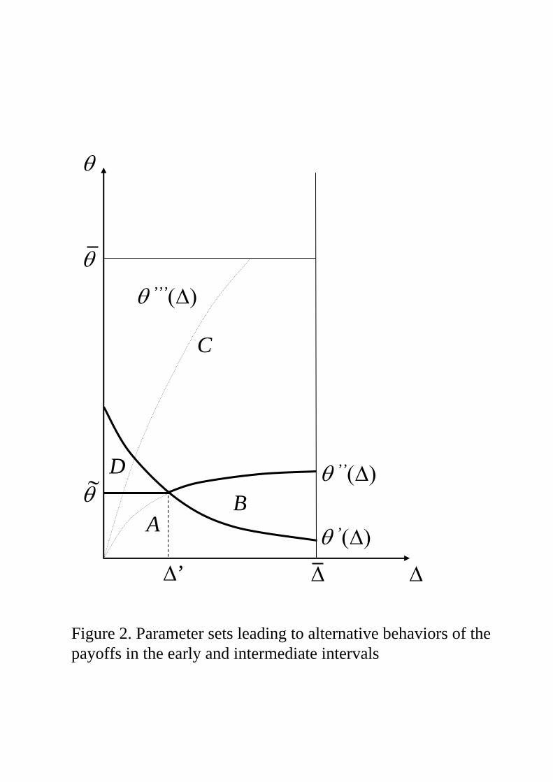
B

ΔΔ’

θ ’’(Δ)θ ∼

θ

Δ

Figure 2. Parameter sets leading to alternative behaviors of the payoffs in the early and intermediate intervals

C

θ ’’’(Δ)

θ ’(Δ)A

D

θ

Panel (c)

T2*− Δ

V1(t1, t1+Δ)

V2(t1, t1+Δ)

t1

T2*− Δ T1

ip_

V1(t1, t1+Δ)

t1

Panel (a)

T2*− Δ T1

ipT1^ T(Δ,θ)

_

V1( t1, t1+Δ)

V2(t1, t1+Δ)

t1

T(Δ,θ)

_T(Δ,θ)

T1^

V2(t1, t1+Δ)

Figure 3: Alternative behaviors for the firms’ discountedpayoffs in the intermediate interval

Panel (b)

Figure 4 Equilibrium selection − minor innovation (x = 0.05)

Δ

Δ

θ

θ

θ

Δ

Panel (a): ρ = 0.01

Panel (b): ρ = 0.05

Panel (c): ρ = 0.09

early eq.

intermediate eq.

intermediate eq.

intermediate eq.

early eq.

late eq.

late eq.

late eq.

Figure 5 Equilibrium selection − major innovation (x = 0.50)

Δ

Δ

θ

θ

θ

Δ

Panel (a): ρ = 0.01

Panel (b): ρ = 0.05

Panel (c): ρ = 0.09

intermediate eq.

intermediate eq.

intermediate eq.

early eq.

early eq.

early eq.

Spillovers, disclosure lags, and incentives to … · Spillovers, disclosure lags, and incentives...

Documents

Transcript of Spillovers, disclosure lags, and incentives to … · Spillovers, disclosure lags, and incentives...