Spike-timing-dependent ensemble encoding by non-classically responsive 1

cortical neurons 2

Authors: Michele N. Insanally1,2

, Ioana Carcea1,2

, Rachel E. Field1,2

, Chris C. Rodgers3, 3

Brian DePasquale4, Kanaka Rajan

5, Michael R. DeWeese

6, Badr F. Albanna

7 and Robert 4

C. Froemke1,2,8

*

5

Affiliations: 6

1 Skirball Institute for Biomolecular Medicine, Neuroscience Institute, Departments of 7

Otolaryngology, Neuroscience and Physiology, New York University School of 8

Medicine, New York, NY, 10016, USA. 9

2 Center for Neural Science, New York University, New York, NY, 10003, USA. 10

3 Department of Neuroscience and Kavli Institute of Brain Science, Columbia University, 11

New York, NY 10032, USA 12

4 Princeton Neuroscience Institute, Princeton University, Princeton NJ, USA 13

5 Department of Neuroscience and Friedman Brain Institute, Icahn School of Medicine at 14

Mount Sinai, One Gustave L. Levy Place, New York, NY, 10029, USA 15

6 Helen Wills Neuroscience Institute and Department of Physics, University of California, 16

Berkeley, CA, 94720, USA 17

7 Department of Natural Sciences, Fordham University, New York, NY, 10023, USA. 18

8 Howard Hughes Medical Institute Faculty Scholar. 19

20

* To whom correspondence should be addressed: 21

Phone: 212-263-4082 22

Email: robert.froemke@med.nyu.edu 23

p. 2 of 95

Neurons recorded in behaving animals often do not discernibly respond to sensory 24

input and are not overtly task-modulated. These non-classically responsive neurons 25

are difficult to interpret and are typically neglected from analysis, confounding 26

attempts to connect neural activity to perception and behavior. Here we describe a 27

trial-by-trial, spike-timing-based algorithm to reveal the coding capacities of these 28

neurons in auditory and frontal cortex of behaving rats. Classically responsive and 29

non-classically responsive cells contained significant information about sensory 30

stimuli and behavioral decisions. Stimulus category was more accurately 31

represented in frontal cortex than auditory cortex, via ensembles of non-classically 32

responsive cells coordinating the behavioral meaning of spike timings on correct but 33

not error trials. This unbiased approach allows the contribution of all recorded 34

neurons – particularly those without obvious task-related, trial-averaged firing rate 35

modulation – to be assessed for behavioral relevance on single trials. 36

p. 3 of 95

Spike trains recorded from the cerebral cortex of behaving animals can be complex, 37

highly variable from trial-to-trial, and therefore challenging to interpret. A fraction of 38

recorded cells typically exhibit trial-averaged firing rates with obvious task-related 39

features and can be considered ‘classically responsive’, such as neurons with tonal 40

frequency tuning in the auditory cortex or orientation tuning in the visual cortex. Another 41

population of responsive cells are modulated by multiple task parameters (‘mixed 42

selectivity cells’), and have recently been shown to have computational advantages 43

necessary for flexible behavior (Rigotti et al., 2013).. However, a substantial number of 44

cells have variable responses that fail to demonstrate firing rates with any obvious trial-45

averaged relationship to task parameters (Jaramillo & Zador, 2010; Olshausen & Field, 46

2006; Raposo, Kaufman, & Churchland, 2014; Rodgers & DeWeese, 2014). These ‘non-47

classically responsive’ neurons are especially prevalent in frontal cortical regions but can 48

also be found throughout the brain, including primary sensory cortex (Hromádka, 49

DeWeese, Zador, & others, 2008; Jaramillo & Zador, 2010; Rodgers & DeWeese, 2014). 50

These response categories are not fixed but can be dynamic, with some cells apparently 51

becoming non-classically responsive during task engagement without impairing 52

behavioral performance (Carcea, Insanally, & Froemke, 2017; Kuchibhotla et al., 2017; 53

Otazu, Tai, Yang, & Zador, 2009). The potential contribution of these cells to behavior 54

remains to a large extent unknown and represents a major conceptual challenge to the 55

field (Olshausen & Field, 2006). 56

57

How do these non-classically responsive cells relate to behavioral task variables on single 58

trials? While there are sophisticated approaches for dissecting the precise correlations 59

p. 4 of 95

between classically responsive cells and task structure (Erlich, Bialek, & Brody, 2011; 60

Jaramillo & Zador, 2010; Kiani & Shadlen, 2009; Murakami, Vicente, Costa, & Mainen, 61

2014; Raposo et al., 2014) there is still a need for complementary and straightforward 62

analytical tools for understanding any and all activity patterns encountered (Jaramillo & 63

Zador, 2010; Raposo et al., 2014; Rigotti et al., 2013). Moreover, most behavioral tasks 64

produce dynamic activity patterns throughout multiple neural circuits, but we lack unified 65

methods to compare activity across different regions, and to determine to what extent 66

these neurons might individually or collectively perform task-relevant computations. To 67

address these limitations, we devised a novel trial-to-trial analysis using Bayesian 68

inference that evaluates the extent to which relative spike timing in single-unit and 69

ensemble responses encode behavioral task variables. 70

71

Results 72

Non-classically responsive cells prevalent in auditory and frontal cortex during 73

behavior 74

We trained 15 rats on an audiomotor frequency recognition go/no-go task (Carcea et al., 75

2017; Froemke et al., 2013; King, Shehu, Roland, Svirsky, & Froemke, 2016; Martins & 76

Froemke, 2015) that required them to nose poke to a single target tone for food reward 77

and withhold from responding to other non-target tones (Figure 1A). Tones were 100 78

msec in duration presented sequentially once every 5-8 seconds at 70 dB sound pressure 79

level (SPL); the target tone was 4 kHz and non-target tones ranged from 0.5-32 kHz 80

separated by one octave intervals. After a few weeks of training, rats had high hit rates to 81

target tones and low false alarm rates to non-targets, leading to high d' values (mean 82

p. 5 of 95

performance shown in Figure 1B; each individual rat included in this study shown in 83

Figure 1-figure supplement 1). 84

85

To correctly perform this task, animals must first recognize the stimulus and then execute 86

an appropriate motor response. We hypothesized that two brain regions important for this 87

behavior are the auditory cortex (AC) and frontal cortical area 2 (FR2). Many but not all 88

auditory cortical neurons respond to pure tones with reliable, short-latency phasic 89

responses (Hromádka et al., 2008; Hubel, Henson, Rupert, & Galambos, 1959; Kadia & 90

Wang, 2002; Merzenich, Knight, & Roth, 1975; Polley, Read, Storace, & Merzenich, 91

2007; Wehr & Zador, 2003; Yaron, Hershenhoren, & Nelken, 2012). These neurons can 92

process sound in a dynamic and context-sensitive manner, and AC cells are also 93

modulated by expectation, attention, and reward structure, strongly suggesting that AC 94

responses are important for auditory perception and cognition (David, Fritz, & Shamma, 95

2012; J. Fritz, Shamma, Elhilali, & Klein, 2003; Hubel et al., 1959; Jaramillo & Zador, 96

2010; Weinberger, 2007). Previously we found that the go/no-go tone recognition task 97

used here is sensitive to AC neuromodulation and plasticity (Froemke et al., 2013). In 98

contrast, FR2 is not thought to be part of the canonical central auditory pathway, but is 99

connected to many other cortical regions including AC (Romanski, Bates, & Goldman-100

Rakic, 1999; Schneider, Nelson, & Mooney, 2014). This region has recently been shown 101

to be involved in orienting responses, categorization of perceptual stimuli, and in 102

suppressing AC responses during movement (Erlich et al., 2011; Hanks et al., 2015; 103

Schneider et al., 2014). These characteristics suggest that FR2 may be important for goal-104

oriented behavior. 105

p. 6 of 95

106

We first asked if activity in AC or FR2 is required for animals to successfully perform 107

this audiomotor task. We implanted cannulas into AC or FR2 (Figure 1-figure 108

supplement 2), and infused the GABA agonist muscimol bilaterally into AC or FR2, to 109

inactivate either region prior to testing behavioral performance. We found that task 110

performance was impaired if either of these regions was inactivated, although general 111

motor functions, including motivation or ability to feed were not impaired (Figure 1-112

figure supplement 3; for AC p=0.03; for FR2 p=0.009 Student’s paired two-tailed t-113

test). Thus activity in both AC and FR2 may be important, perhaps in different ways, for 114

successful performance on this task. We note that a previously published study (Gimenez, 115

Lorenc, & Jaramillo, 2015) observed a more modest effect of muscimol-based 116

inactivation of auditory cortex (although we used a separate task and higher dose of 117

muscimol than that study which might contribute to this difference). 118

119

Once animals reached behavioral criteria (hit rates ≥70% and d’ values ≥1.5), they were 120

implanted with tetrode arrays in either AC or FR2 (Figure 1- figure supplement 4). 121

After recovery, we made single-unit recordings from individual neurons or small 122

ensembles of 2-8 cells during task performance. The trial-averaged responses of some 123

cells exhibited obvious task-related features: neuronal activity was tone-modulated 124

compared to inter-trial baseline activity (Figure 1C) or gradually changed over the 125

course of the trial as measured by a ramping index (Figure 1D; hereafter referred to as 126

‘ramping activity’). However, 60% of recorded cells were non-classically responsive in 127

that they were neither tone modulated nor ramping according to statistical criteria 128

p. 7 of 95

(Figure 1E, 1F; Figure 1-figure supplement 5; 64/103 AC cells and 43/74 FR2 cells 129

from 15 animals had neither significant tone-modulated activity or ramping activity; pre 130

and post-stimulus mean activity compared via subsampled bootstrapping and considered 131

significant when p<0.05; ramping activity measured with linear regression and 132

considered significant via subsampled bootstrapping when p<0.05 and r>0.5; for overall 133

population statistics see Figure 1-figure supplement 6). While the fraction of non-134

classically responsive AC neurons observed is consistent with previous studies that use 135

different auditory stimuli or behavioral paradigms (Jaramillo & Zador, 2011; Rodgers & 136

DeWeese, 2014), this definition does not preclude the possibility that non-classically 137

responsive cells can be driven by other acoustic stimuli or behavioral paradigms. 138

139

Novel single-trial, ISI-based algorithm for decoding non-classically responsive 140

activity 141

Given that the majority of our recordings were from non-classically responsive cells, we 142

developed a general method for interpreting neural responses even when trial-averaged 143

responses were not obviously task-modulated which allowed us to compare coding 144

schemes across different brain regions (here, AC and FR2). The algorithm is agnostic to 145

the putative function of neurons as well as the task variable of interest (here, stimulus 146

category or behavioral choice). 147

148

Our algorithm empirically estimates the interspike interval (ISI) distribution of individual 149

neurons to decode the stimulus category (target or non-target) or behavioral choice (go or 150

no-go) on each trial via Bayesian inference. The ISI was chosen because its distribution 151

p. 8 of 95

could vary between task conditions even without changes in the firing rate – building on 152

previous work demonstrating that the ISI distribution contains complementary 153

information to the firing rate (Lundstrom & Fairhall, 2006; Reich, Mechler, Purpura, & 154

Victor, 2000; Zuo et al., 2015). The distinction between the ISI distribution and trial-155

averaged firing rate is subtle, yet important. While the ISI is obviously closely related to 156

the instantaneous firing rate, decoding with the ISI distribution is not simply a proxy for 157

using the time-varying, trial-averaged rate. To demonstrate this we constructed three 158

model cells: a stimulus-evoked cell with distinct target and non-target ISI distributions 159

(Figure 2A), a stimulus-evoked cell with identical ISI distributions (Figure 2B), and a 160

non-classically responsive cell with distinct target and non-target ISI distributions 161

(Figure 2C). These models clearly demonstrate that trial-averaged rate modulation can 162

occur with or without corresponding differences in the ISI distributions and cells without 163

apparent trial-averaged rate-modulation can nevertheless have distinct ISI distributions. 164

Taken together, these examples demonstrate that the ISI distribution and trial-averaged 165

firing rate capture different spike train statistics. This has important implications for 166

decoding non-classically responsive cells that by definition do not exhibit large firing rate 167

modulations but nevertheless may contain information latent in their ISI distributions. 168

169

For each recorded neuron, we built a library of ISIs observed during target trials and a 170

library for non-target trials from a set of ‘training trials’. Two different cells from AC are 171

shown in Figure 3A and Figure 3-figure supplement 1A-D, and another cell from FR2 172

is shown in Figure 3-figure supplement 1E-H. These libraries were used to infer the 173

probability of observing an ISI during a particular trial type (Figure 3B,C; Figure 3-174

p. 9 of 95

figure supplement 1C,G; left panels show target in red and non-target in blue). These 175

conditional probabilities were inferred using non-parametric statistical methods to 176

minimize assumptions about the underlying process generating the ISI distribution and 177

better capture the heterogeneity of the observed ISI distributions (Figure 3B; Figure 3-178

figure supplement 1C,G). We verified that our observed distributions were better 179

modeled by non-parametric methods rather than standard parametric methods (e.g. rate-180

modulated Poisson process; Figure 3-figure supplement 2). Specifically, we found the 181

distributions using Kernel Density Estimation where the kernel bandwidth for each 182

distribution was set using 10-fold cross-validation. To accommodate any non-stationarity, 183

these ISI distributions were calculated in 1 second long sliding windows recalculated 184

every 100 ms over the course of the trial. We then used these training set probability 185

functions to decode a spike train from a previously unexamined individual trial from the 186

set of remaining ‘test trials’. This process was repeated 124 times using 10-fold cross-187

validation with randomly generated folds. 188

189

Importantly, while the probabilities of observing particular ISIs on target and non-target 190

trials were similar (Figure 3B; Figure 3-figure supplement 1C,G), small differences 191

between the curves carried sufficient information to allow for decoding. To characterize 192

these differences, we used the weighted log likelihood ratio (W. LLR; Figure 3C; Figure 193

3-figure supplement 1C,G) to clearly represent which ISIs suggested target (W. LLR 194

>0) or non-target (W. LLR <0) stimulus categories. Our algorithm relies only on 195

statistical differences between task conditions; therefore, the W. LLR summarizes all 196

spike timing information necessary for decoding. Similar ISI libraries were also 197

p. 10 of 95

computed for behavioral choice categories (Figure 3B,C; Figure S3-figure supplement 198

1C,G; right panels show go decision in green and no-go in purple). These examples 199

clearly illustrate that the relationship between the ISIs and task variables cannot simply 200

be approximated by an ISI or firing rate threshold where short ISIs imply a one task 201

variable and longer ISIs imply another: in the cell shown in Figure 3, short ISIs (ISI <50 202

msec) indicated non-target, medium ISIs (50 msec < ISI < 100 msec) indicated target, 203

and longer ISIs indicated non-target (100 msec < ISI). 204

205

The algorithm uses the statistical prevalence of certain ISI values under particular task 206

conditions (in this case the ISIs accompanying stimulus category or behavioral choice), to 207

infer the task condition for each trial. Each trial begins with equally uncertain 208

probabilities about the stimulus categories (i.e., p(target) = p(non-target) = 50%). As each 209

ISI is observed sequentially within the trial, the algorithm applies Bayes’ rule to update 210

p(target|ISI) and p(non-target|ISI) using the likelihood of the ISI under each stimulus 211

category (p(ISI|target) and p(ISI|non-target) (Figure 3B-D). As these functions were 212

estimated in 1 second long sliding windows, each ISI was assessed using the distribution 213

that placed the final spike closest to the center of the sliding window. As shown for one 214

trial of the example cell in Figure 3D, ISIs observed between 0-1.0 seconds consistently 215

suggested the presence of the target tone, whereas ISIs observed between 1.0-1.4 seconds 216

suggested the non-target category thereby also necessarily reducing the belief that a target 217

tone was played (Figure 3D, top trace). These ISI likelihood functions consider each ISI 218

to be independent of previous ISIs and therefore ignore correlations between ISIs. After 219

this process was completed for all ISIs in the particular trial, we obtained the probability 220

p. 11 of 95

of a non-target tone and a target tone as a function of time during the trial (Figure 3D). 221

Because it is particularly challenging to dissociate choice from motor execution or 222

preparatory motor activity in this task paradigm, the prediction for the entire trial 223

p(target|ISI) is evaluated at the end of the trial (in the example trial, p(target|ISI) = 61%; 224

Figure 3D). This process is repeated for the behavioral choice (Figure 3B-D; right 225

panels; trials separated according to go, no-go; probabilities of ISIs in each condition 226

generated; conditional probabilities used as likelihood function to predict behavioral 227

choice on a given trial). The single-trial decoding performance of each neuron is then 228

averaged over all trials as a measure of the overall ability of each neuron to distinguish 229

behavioral conditions (Figure 4A). Note that this measure not only takes into account 230

whether the algorithm was correct on individual trials (i.e. target vs. non-target), but also 231

its prediction certainty. 232

233

Non-classically responsive cells contain spike-timing-based task information 234

Can we uncover task information from non-classically responsive cells? We found that 235

non-classically responsive cells in both AC and FR2 provided significant spike-timing-236

based information about each task variable (Figure 4A,B, red; Figure 4-figure 237

supplement 1). The ability to decode was poorly explained by the average firing rate 238

(Figure 4-figure supplement 2A-F, 0.30 < r

< 0.46), z-score (Figure 4-figure 239

supplement 2G-I, -0.05 < r < 0.05), and ramping activity (Figure 4-figure supplement 240

2J, -0.02 < r < 0.28). Stimulus decoding performance was also independent of receptive 241

field properties including best frequency and tuning curve bandwidth for AC neurons 242

(Figure 4-figure supplement 3). 243

p. 12 of 95

244

We also observed that task information was distributed across both AC and FR2, and 245

neural spike trains from individual units were multiplexed in that they often encoded 246

information about both stimulus category and choice simultaneously (Figure 4B, Table 247

1). Given the strong correlation between stimulus and choice variables in the task design, 248

it is difficult to fully separate information about one variable from information about the 249

other. To establish that multiplexing was not simply a byproduct of this correlation, an 250

independent measure of multiplexing relying on multiple regression was applied (Figure 251

4-figure supplement 4). This analysis confirmed that the information revealed by our 252

algorithm about a behavioral variable was primarily a reflection of that variable and not 253

simply an indirect measure of the other, correlated variable. This analysis establishes that 254

a certain degree of separability is possible and demonstrates that the multiplexing 255

observed in our decoding results is unlikely to be a trivial byproduct of correlations in the 256

task variables. 257

258

Despite the broad sharing of information about behavioral conditions, there were notable 259

systematic differences between AC and FR2. Surprisingly, neurons in FR2 were more 260

informative about stimulus category than AC, and AC neurons were more informative 261

about choice than stimulus category (Figure 4A, pAC=0.016, pstim=0.0013, Mann-262

Whitney U test, two-sided). Both of these observations would not have been detected at 263

the level of the PSTH, as most cells in AC were non-classically responsive for behavioral 264

choice (no ramping activity, 91/103), yet our decoder revealed that these same cells were 265

as informative as choice classically responsive cells (Figure 4C, p=0.32 Mann-Whitney 266

p. 13 of 95

U test, two-sided; red circles indicate cells non-classically responsive for both variables, 267

dark-red cells are choice non-classically responsive, and black cells are classically 268

responsive). Similarly, most cells in FR2 were sensory non-classically responsive (not 269

tone modulated, 60/74), yet contained comparable stimulus information to sensory 270

classically responsive cells (Figure 4D, p=0.29 Mann-Whitney U test, two-sided; red 271

cells are non-classically responsive for both variables, dark-red cells are sensory non-272

classically responsive, black cells are classically responsive). 273

274

To assess the statistical significance of these results, we tested our algorithm on two 275

shuffled data sets. First, we ran our analysis using synthetically-generated trials that 276

preserved trial length but randomly sampled ISIs with replacement from those observed 277

during a session without regard to condition (Figure 4E). Second, we left trial activity 278

intact, but permuted the stimulus category and choice for each trial (Figure 4F). We 279

restricted analysis to cells with decoding performance significantly different from 280

synthetic spike trains (all cells in Figure 4A-D significantly different from synthetic 281

condition shown in Figure 4E, p<0.05, bootstrapped 1240 times). 282

283

To directly assess the extent to which information captured by the ISI distributions in our 284

data set was distinct from the time-varying rate, we compared the performance from our 285

ISI-based decoder to a conventional rate-modulated (inhomogeneous) Poisson decoder 286

(Rieke, Warland, de de Ruyter van Steveninck, & Bialek, 1999) which assumes that 287

spikes are produced randomly with an instantaneous probability equal to the time-varying 288

firing rate. As our model cells illustrate (Figure 2), it is possible to decode using the ISI 289

p. 14 of 95

distributions even when firing rates are uninformative (Figure 5A). When applied to our 290

dataset, the ISI-based decoder generally outperformed this conventional rate-based 291

decoder confirming that ISIs capture information distinct from that of the firing rate 292

(Figure 5B; Overall stimulus decoding performance: pAC=0.0001, pFR2=8×10-6

; Overall 293

choice decoding performance pAC=0.0057, pFR2=0.02, Mann-Whitney U test, two-sided). 294

Moreover, comparing single trial decoding outcomes demonstrated weak to no 295

correlations between the ISI-based decoder and the conventional rate decoder, further 296

underscoring that these two methods rely on different features of the spike train to decode 297

(Figure 5C; stimulus medians: AC=0.10 FR2=0.11; choice medians: AC=0.07, 298

FR2=0.08). 299

300

We hypothesize that ISI-based decoding is biologically plausible. Short-term synaptic 301

plasticity and synaptic integration provide powerful mechanisms for differential and 302

specific spike-timing-based coding. We illustrated this capacity by making whole-cell 303

recordings from AC neurons in vivo and in brain slices (Figure 5-figure supplement 304

1A,B), as well as in FR2 brain slices (Figure 5-figure supplement 1C). In each case, 305

different cells could have distinct response profiles to the same input pattern, with similar 306

overall rates but different spike timings. 307

308

Moreover, we note that this type of coding scheme requires few assumptions about 309

implementation, and does not require additional separate integrative processes to 310

compute rates or form generative models. Thus ISI-based decoding coding could be 311

generally applicable across brain areas, as demonstrated here for AC and FR2. 312

p. 15 of 95

313

Non-classically responsive cells encode selection rule information in a novel task-314

switching paradigm 315

To further demonstrate the generalizability and utility of our approach, we applied our 316

decoding algorithm to neurons that were found to be non-classically responsive in a 317

previously published study (Rodgers & DeWeese, 2014). In this study, rats were trained 318

on a novel auditory stimulus selection task where depending on the context animals had 319

to respond to one of two cues while ignoring the other. Rats were presented with two 320

simultaneous sounds (a white noise burst and a warble). In the “localization” context the 321

animal was trained to ignore the warble and respond to the location of the white noise 322

burst and in the “pitch” context it was trained to ignore the location of the white noise 323

burst and respond to the pitch of the warble (Figure 6A). Using our algorithm, we found 324

significant stimulus and choice-related information in the activity of non-classically 325

responsive cells that displayed no stimulus modulation nor ramping activity in the firing 326

rate (Figure 6B-D). The main finding of the study is that the pre-stimulus activity in both 327

primary auditory cortex and prefrontal cortex encodes the selection rule (i.e. activity 328

reflects whether the animal is in the localization or pitch context). This conclusion was 329

entirely based on a difference in pre-stimulus firing rate between the two contexts. The 330

authors reported, but did not further analyze, cells that did not modulate their pre-331

stimulus firing rate. In our nomenclature these cells are “non-classically responsive for 332

the selection rule”. Using our algorithm we found that the ISI distributions of these cells 333

encoded the selection rule and were significantly more informative than the classically 334

responsive cells (Figure 6E, pAC=5×10-6

, pPFC<0.0002, Mann-Whitney U test, two-335

p. 16 of 95

sided). This surprising result demonstrates that our algorithm generalizes to novel 336

datasets, and may be used to uncover coding for cognitive variables beyond those 337

apparent from conventional trial-averaged, rate-based analyses. Furthermore, these 338

results indicate that as task complexity increases non-classically responsive cells are 339

differentially recruited for successful task execution. 340

341

Non-classically responsive ensembles are better predictors of behavioral errors 342

Downstream brain regions must integrate the activity of many neurons and this ISI-based 343

approach naturally extends to simultaneously recorded ensembles. We therefore asked 344

whether using small ensembles would change or improve decoding. To decode from 345

ensembles, likelihood functions from each cell were calculated independently as before, 346

but were used to simultaneously update the task condition probabilities (p(target | ISI) 347

and p(go | ISI)) on each trial (Figure 7A). Analyzing ensembles of 2-8 neurons in AC 348

and FR2 significantly improved decoding for both variables in FR2 and stimulus 349

decoding in AC (Figure 7B, pAC stim=0.04, pFR2 stim=1×10-5

, pAC=0.29, pFR2 choice=7×10-5

, 350

Mann-Whitney U test, two-sided). This was not a trivial consequence of using more 351

neurons, as the information provided by individual ISIs on single trials can be 352

contradictory (e.g., compare LLR functions in Figure 3C and Figure S3-figure 353

supplement 1C for 50 ms < ISIs < 120 ms). For ensemble decoding to improve upon 354

single neuron decoding, the ISIs of each member of the ensemble must indicate the same 355

task variable. 356

357

p. 17 of 95

Can our decoding method predict errors on a trial-by-trial basis? In general, trial-358

averaged PSTHs did not reveal systematic differences between correct and error trials 359

(Figure 7-figure supplement 1). However, when we examined single-trial performance 360

with our algorithm, ensembles of neurons in AC and FR2 predicted behavioral errors 361

(Figure 7C). In general, ensembles in AC predicted behavioral errors significantly better 362

than those in FR2 (Figure 7C, for 3-member ensembles: p=1.2×10-5

, for 4-member 363

ensembles: p=0.03, Mann-Whitney U test, two-sided). Interestingly, decoding with an 364

increasing number of non-classically responsive cells improved error prediction in both 365

AC and FR2 (Figure 7D, (pAC=0.013, pFR2=0.046, Welch’s t-test). 366

367

Timing-dependent ensemble consensus-building dynamics underlie task information 368

While improvements were seen in decoding performance with increasing ensemble size, 369

the ISI distributions/ISI-based likelihood functions were highly variable across individual 370

ensemble members. Thus, we wondered if there was task-related structure in the timing 371

of population activity that evolved over the course of the trial to instantiate behavior. To 372

answer this question, we examined whether local ensembles share the same 373

representation of task variables over the course of the trial. Do they “reach consensus” on 374

how to represent task variables using the ISI (Figure 8A)? Without consensus, a 375

downstream area would need to interpret ensemble activity using multiple disparate 376

representations rather than one unified code (Figure 8B). The firing rates and ISI 377

distributions of simultaneously-recorded units were generally variable across cells 378

requiring an exploratory approach to answer this question (Figure 8C, example three-379

member ensemble with heterogeneous conditional ISI distributions). Therefore, we 380

p. 18 of 95

examined changes in the distributions of ISIs across task conditions, asking how the 381

moment-to-moment changes in the log-likelihood ratio (LLR) of each cell were 382

coordinated to encode task variables (Figure 8C). We focused on the LLR because it 383

quantifies how the ISI represents task variables for a given cell and summarizes all spike 384

timing information needed by our algorithm (or a hypothetical downstream cell) to 385

decode. 386

387

We examined how ensembles coordinate their activity moment-to-moment over the 388

course of the trial by quantifying the similarity of the LLRs across cells in a sliding 389

window. Similarity was assessed by summing the LLRs of ensemble members, 390

calculating the total area underneath the resulting curve, and normalizing this value by 391

the sum of the areas of each individual LLR. We refer to this quantified similarity as 392

‘consensus’; a high consensus value indicates that ensemble members have similar LLRs 393

and therefore have a similar representation of task variables (Figure 8D). We should 394

emphasize that successful ensemble decoding (Figure 7) does not require the LLRs of 395

ensemble members to be related in any way; therefore, structured LLR dynamics (Figure 396

8) are not simply a consequence of how our algorithm is constructed. 397

398

While the conventional trial-averaged PSTH of non-classically responsive ensembles 399

recorded in AC and FR2 showed no task-related modulation, our analysis revealed 400

structured temporal dynamics of the LLRs (captured by the consensus value). On correct 401

trials, we observe a trajectory of increasing consensus at specific moments during the trial 402

signifying a dynamically created, shared ISI representation of task variables. In FR2, 403

p. 19 of 95

sensory non-classically responsive ensembles (ensembles in which at least two out of 404

three cells were not tone-modulated) encode stimulus information using temporally-405

precise stimulus-related dynamics on correct trials. The stimulus representation of 406

sensory non-classically responsive ensembles reached consensus rapidly after stimulus 407

onset followed by divergence (Figure 8E, stimulus-aligned, solid line, consensus, t = 0 408

to 0.42 s, pSNR = 3.9×10-4

Wilcoxon test with Bonferroni correction, two-sided). Sensory 409

classically responsive ensembles in AC increased consensus beyond stimulus 410

presentation, reaching a maximum ~750 ms after tone onset on correct trials (Figure 8E 411

stimulus-aligned, dotted line, consensus, t = 0 to 0.81 s, pSR = 0.14 Wilcoxon test with 412

Bonferroni correction, two-sided). For choice-related activity, choice non-classically 413

responsive ensembles in both regions as well as choice classically responsive ensembles 414

in FR2 each reached consensus within 500 ms of the behavioral response (Figure 8E, 415

response-aligned, consensus, t = -1.0 to 0.0 s, pCNR = 2.0×10-5

, pCR = 0.12 Wilcoxon test 416

with Bonferroni correction, two-sided). Importantly, this temporally precise pattern of 417

consensus building is not present on error trials. On error trials, stimulus consensus 418

dynamics decreased over the course of the trial whereas choice dynamics did not display 419

a systematic increase with the exception of choice non-classically responsive ensembles 420

in AC which remained systematically lower than correct trials (Figure 8F, consensus, 421

correct trials vs. error trials, stimulus: pSNR= 0.007, pSR = 0.065, choice: pCNR = 0.0048, 422

pCR = 0.065 Mann-Whitney U test, two-sided, consensus on error trials, t = 0 to 0.42 s, 423

pSNR = 1.3×10-33

, t = -1.0 to 0 s, pCNR = 0.032, pCR = 0.14 Wilcoxon test with Bonferroni 424

correction, two-sided). The observed increases in ensemble consensus on correct trials 425

p. 20 of 95

(while failing do so on error trials) suggests that achieving a shared ISI representation of 426

task variables may be relevant for successful task execution. 427

428

These results reveal that consensus-building and divergence occur at key moments during 429

the trial for successful execution of behavior in a manner that is invisible at the level of 430

the PSTH. As sensory and choice non-classically responsive ensembles participated in 431

these dynamics, changes in the consensus value cannot simply be a byproduct of 432

correlated firing rate modulation due to tone-evoked responses or ramping. While 433

consensus-building can only indicate a shared representation, divergence can indicate one 434

of two things: (1) the LLRs of each cell within an ensemble are completely dissimilar or 435

(2) they are ‘out of phase’ with one another – the LLRs partition the ISIs the same way 436

(Figure 8D, dotted lines), but the same ISIs code for opposite behavioral variables. This 437

distinction is important because (2) implies coordinated structure of ensemble activity 438

(the partitions of the ISI align) whereas (1) does not. To distinguish between these two 439

possibilities we used the ‘unsigned consensus’, a second measure sensitive to the ISI 440

partitions but insensitive to the sign of the LLR. Both ‘in phase’ and perfectly ‘out of 441

phase’ LLRs would produce an unsigned consensus of 1 whereas unrelated LLRs would 442

be closer to 0 (Figure 8D). For example, in the second row of Figure 8D, both cells 443

agree that ISIs < 100 ms indicate one stimulus category and ISIs > 100 ms indicate 444

another, but they disagree about which set of ISIs mean target and which mean non-445

target. This results in a consensus value of 0 (out of phase) but an unsigned consensus 446

value of 1. 447

448

p. 21 of 95

Using this metric, we found that the unsigned consensus pattern for non-classically 449

responsive ensembles (ensembles with two or more non-classically responsive members) 450

were shared between AC and FR2 – increasing until ~750 ms after tone onset on correct 451

trials (Figure 8G, stimulus-aligned, consensus, t = 0 to 0.89 s, p = 1.7×10-5

Wilcoxon 452

test, two-sided). Non-classically responsive ensembles in AC and FR2 also increased 453

their unsigned consensus immediately before behavioral response (although values in AC 454

were lower overall; Figure 8G, response-aligned, consensus, t = -1.0 to 0.0 s, p = 455

0.0011 Wilcoxon test, two-sided). This pattern of consensus-building was only present on 456

correct trials. On error trials unsigned consensus values did not systematically increase 457

(Figure 8H, consensus compared to error trials, p = 1.9×10-9

Mann-Whitney U test, 458

two-sided) suggesting that behavioral errors might result from a general lack of 459

consensus between ensemble members. In summary, we have shown that cells which 460

appear unmodulated during behavior do not encode task information independently, but 461

do so by synchronizing their representation of behavioral variables dynamically during 462

the trial. 463

464

Discussion 465

Using a straightforward, single-trial, ISI decoding algorithm that makes few assumptions 466

about the proper model for neural activity, we found task-specific information 467

extensively represented by non-classically responsive neurons in both AC and FR2 that 468

lacked conventional task-related, trial-averaged firing rate modulation. The complexity of 469

single-trial spiking patterns and the apparent variability between trials led to the 470

development of this novel decoding method. Furthermore, the heterogeneity in the 471

p. 22 of 95

observed ISI distributions within and across brain regions precluded a straightforward 472

interpretation of these distributions and instead suggested an approach which focused on 473

whether and when these distributions are shared in local ensembles via consensus-474

building. 475

476

The degree to which single neurons were task-modulated was uncorrelated with 477

conventional response properties including frequency tuning. AC and FR2 each represent 478

both task-variables; furthermore, in both regions we identified many multiplexed neurons 479

that simultaneously represented the sensory input and the upcoming behavioral choice 480

including non-classically responsive cells. This highlights that the cortical circuits that 481

generate behavior exist in a distributed network – blurring the traditional modular view of 482

sensory and frontal cortical regions. 483

484

Most notably, FR2 has a better representation of task-relevant auditory stimuli than AC. 485

The prevalence of stimulus information in FR2 might be surprising given that AC 486

reliably responds to pure tones in untrained animals; however, when tones take on 487

behavioral significance, this information is encoded more robustly in frontal cortex, 488

suggesting that this region is critical for identifying the appropriate sensory-motor 489

association. Furthermore, the stark improvement in stimulus encoding for small 490

ensembles in FR2 suggests that task-relevant stimulus information is reflected more 491

homogeneously in local firing activity across FR2 (perhaps through large scale ensemble 492

consensus-building) while this information is reflected in a more complex and distributed 493

manner throughout AC. 494

p. 23 of 95

495

We have identified task-informative non-classically responsive neurons recorded while 496

animals performed a frequency recognition task or a task-switching paradigm. This does 497

not preclude the possibility that these cells are driven by other acoustic stimuli or in other 498

behavioral contexts; however, determining the significance of non-classically responsive 499

activity must ultimately be considered in the specific behavioral context in question, as 500

their role may be dynamic and context dependent. 501

502

The finding that the ISI-based approach of our algorithm is not reducible to rate despite 503

their close mathematical relationship raises the question of how downstream regions 504

could respond preferentially to specific ISIs. Our whole-cell recordings from both AC 505

and FR2 demonstrate that different postsynaptic cells can respond differently to the same 506

input pattern with a fixed overall rate, emphasizing the importance of considering a code 507

sensitive to precise spike-timing perhaps via mechanisms of differential short-term 508

plasticity such as depression and facilitation (Figure 5-figure supplement 1). 509

Furthermore, this is supported by experimental and theoretical work showing that single 510

neurons can act as resonators tuned to a certain periodicity of firing input (Izhikevich, 511

2000). This view could also be expanded to larger neuronal populations comprised of 512

feedback loops that would resonate in response to particular ISIs. In this case, cholinergic 513

neuromodulation could offer a mechanism for adjusting the sensitivities of such a 514

network during behavior on short time-scales by providing rapid phasic signals (Hangya, 515

Ranade, Lorenc, & Kepecs, 2015). 516

517

p. 24 of 95

Our consensus results reveal dynamic changes in the relationship between the LLRs of 518

ensemble members. How might such a downstream resonator interpret a given ISI in the 519

context of these dynamics? Our consensus analysis provides one possible answer: 520

downstream neurons may be attuned to the ISIs specified by the consensus LLR of an 521

ensemble. In such a model, an ensemble would have the strongest influence on 522

downstream activity when they reach high consensus. We additionally hypothesize that 523

mechanisms of long-term synaptic plasticity such as spike-timing-dependent plasticity 524

can redistribute synaptic efficacy, essentially changing the dynamics of short-term 525

plasticity independent from overall changes in amplitudes (Markram & Tsodyks, 1996). 526

Thus, after training, downstream neurons do not need to continually change the readout 527

mechanism- rather, the upstream and downstream components might be modified 528

together by cortical plasticity during initial phases of behavioral training. This would set 529

the ISI distributions appropriate for firing of task-relevant downstream neurons, which 530

would ensure that ensemble consensus is reached for correct sensory processing in 531

highly-trained animals. 532

533

It is still unclear what the relevant timescales of decoding might be in relation to 534

phenomena such as membrane time constants, periods of oscillatory activity, and 535

behavioral timescales. Given that our ISI-based decoder and conventional rate-modulated 536

decoders reveal distinct information, future approaches might hybridize these rate-based 537

and temporal-based decoding methods to span multiple timescales. Other recent studies 538

have also contributed to our understanding of non-classically responsive activity, by 539

evaluating firing rates or responses from calcium imaging to demonstrate how 540

p. 25 of 95

correlations with classically responsive activity may contribute to the linear separability 541

of ensemble responses (Leavitt, Pieper, Sachs, & Martinez-Trujillo, 2017; Zylberberg, 542

2018). 543

544

We have shown that underlying the task-relevant information encoded by each ensemble 545

is a rich set of consensus-building dynamics that is invisible at the level of the PSTH. 546

Ensembles in both FR2 and AC underwent stimulus and choice-related consensus 547

building that was only observed when the animal correctly executed the task. Moreover, 548

non-classically responsive cells demonstrated temporal dynamics synchronized across 549

regions which were distinct from classically responsive ensembles. These results 550

underscore the importance of measuring neural activity in behaving animals and using 551

unbiased and generally-applicable analytical methods, as the response properties of 552

cortical neurons in a behavioral context become complex in ways that challenge our 553

conventional assumptions (Carcea et al., 2017; J. B. Fritz, David, Radtke-Schuller, Yin, 554

& Shamma, 2010; Kuchibhotla et al., 2017; Otazu et al., 2009). 555

556

p. 26 of 95

Methods 557

Key resources table 558

Reagent type

(species) or resource Designation

Source

or

reference

Identifiers Additional information

strain, strain

background (Rattus

norvegicus

domesticus, males and

females)

Sprague-

Dawley, rats

Charles

River,

Taconic

NTac:SD

chemical compound,

drug Muscimol

Sigma-

Aldrich

InChi:ZJQHPWUVQPJPQT-

UHFFFAOYSA-N;

SID:24896662

software, algorithm

Single-trial

Bayesian

decoding

algorithm

newly

created N/A https://github.com/badralbanna/Insanally2017

other

Rodgers &

DeWeese

2014 dataset

CRCNS pfc-1 http://crcns.org/data-sets/pfc/pfc-1

559

Behavior 560

All animal procedures were performed in accordance with National Institutes of Health 561

standards and were conducted under a protocol approved by the New York University 562

School of Medicine Institutional Animal Care and Use Committee. We used 23 adult 563

Sprague-Dawley male and female rats (Charles River) in the behavioral studies. Animals 564

were food restricted and kept at 85% of their initial body weight, and maintained at a 12 565

hr light/12 hr dark cycle. 566

Animals were trained on a go/no-go audiomotor task (Carcea et al., 2017; 567

Froemke et al., 2013). Operant conditioning was performed within 12” L x 10” W x 568

10.5” H test chambers with stainless steel floors and clear polycarbonate walls (Med 569

Associates), enclosed in a sound attenuation cubicle and lined with soundproofing 570

acoustic foam (Med Associates). The nose and reward ports were both arranged on one of 571

p. 27 of 95

the walls with the speaker on the opposite wall. The nose port, reward port, and the 572

speaker were controlled and monitored with a custom-programmed microcontroller. Nose 573

port entries were detected with an infrared beam break detector. Auditory stimuli were 574

delivered through an electromagnetic dynamic speaker (Med Associates) calibrated using 575

a pressure field microphone (ACO Pacific). 576

Animals were rewarded with food for nose poking within 2.5 seconds of 577

presentation of the target tone (4 kHz) and given a short 7-second time-out for incorrectly 578

responding to non-target tones (0.5, 1, 2, 8, 16, 32 kHz). Incorrect responses include 579

either failure to enter the nose port after target tone presentation (miss trials) or entering 580

the nose port after non-target tone presentation (false alarms). Tones were 100 msec in 581

duration and sound intensity was set to 70 dB SPL. Tones were presented randomly with 582

equal probability such that each stimulus category was presented. The inter-trial interval 583

delays used were 5, 6, 7, or 8 seconds. 584

p. 28 of 95

For experiments involving muscimol, we implanted bilateral cannulas in either 585

FR2 (+2.0 to +4.0 mm AP, ±1.3 mm ML from Bregma) of 7 animals or AC (-5.0 to -5.8 586

mm AP, 6.5-7.0 mm ML from Bregma) of 3 animals. We infused 1 μL of muscimol per 587

side into FR2 or infused 2 μL of muscimol per side into AC, at a concentration of 1 588

mg/mL. For saline controls, equivalent volumes of saline were infused in each region. 589

Behavioral testing was performed 30-60 minutes after infusions. Power analysis was 590

performed to determine sample size for statistical significance with a power of : 0.8; 591

these studies required at least 3 animals, satisfied in the experiments of Figure 1-figure 592

supplement 3B,E. For motor control study, animals could freely nose poke for food 593

reward without presentation of auditory stimuli after muscimol and saline infusion. 594

595

Implant preparation and surgery 596

Animals were implanted with microdrive arrays (Versadrive-8 Neuralynx) in either AC 597

(8 animals) or FR2 (7 animals) after reaching behavioral criteria of d’ ≥ 1.0. For surgery, 598

animals were anesthetized with ketamine (40 mg/kg) and dexmedetomidine (0.125 599

mg/kg). Stainless steel screws and dental cement were used to secure the microdrive to 600

the skull, and one screw was used as ground. Each drive consisted of 8 independently 601

adjustable tetrodes. The tetrodes were made by twisting and fusing four polyimide-coated 602

nichrome wires (Sandvik Kanthal HP Reid Precision Fine Tetrode Wire; wire diameter 603

12.5 μm). The tip of each tetrode was gold-plated to an impedance of 300-400 kOhms at 604

1 kHz (NanoZ, Neuralynx). 605

606

p. 29 of 95

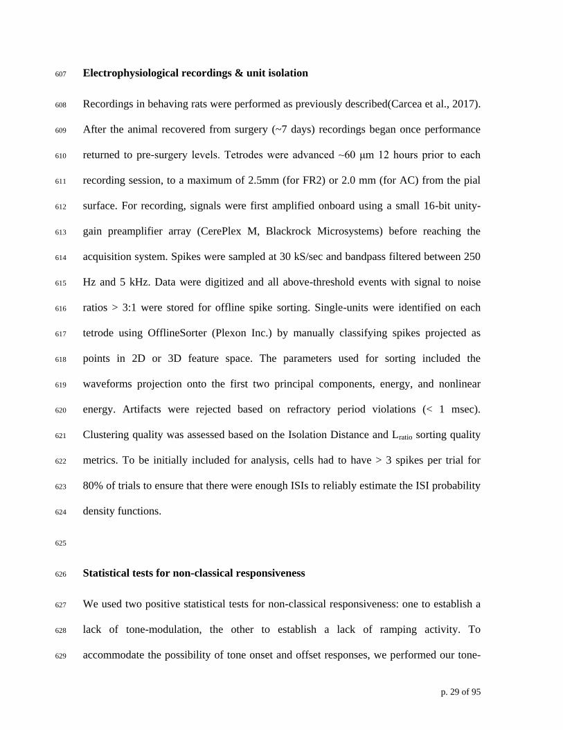
Electrophysiological recordings & unit isolation 607

Recordings in behaving rats were performed as previously described(Carcea et al., 2017). 608

After the animal recovered from surgery (~7 days) recordings began once performance 609

returned to pre-surgery levels. Tetrodes were advanced ~60 μm 12 hours prior to each 610

recording session, to a maximum of 2.5mm (for FR2) or 2.0 mm (for AC) from the pial 611

surface. For recording, signals were first amplified onboard using a small 16-bit unity-612

gain preamplifier array (CerePlex M, Blackrock Microsystems) before reaching the 613

acquisition system. Spikes were sampled at 30 kS/sec and bandpass filtered between 250 614

Hz and 5 kHz. Data were digitized and all above-threshold events with signal to noise 615

ratios > 3:1 were stored for offline spike sorting. Single-units were identified on each 616

tetrode using OfflineSorter (Plexon Inc.) by manually classifying spikes projected as 617

points in 2D or 3D feature space. The parameters used for sorting included the 618

waveforms projection onto the first two principal components, energy, and nonlinear 619

energy. Artifacts were rejected based on refractory period violations (< 1 msec). 620

Clustering quality was assessed based on the Isolation Distance and Lratio sorting quality 621

metrics. To be initially included for analysis, cells had to have > 3 spikes per trial for 622

80% of trials to ensure that there were enough ISIs to reliably estimate the ISI probability 623

density functions. 624

625

Statistical tests for non-classical responsiveness 626

We used two positive statistical tests for non-classical responsiveness: one to establish a 627

lack of tone-modulation, the other to establish a lack of ramping activity. To 628

accommodate the possibility of tone onset and offset responses, we performed our tone-629

p. 30 of 95

modulation test on a 100 ms long tone presentation window as well as the 100 ms 630

window immediately after tone presentation. The test compared the number of spikes 631

during each of these windows to inter-trial baseline activity as measured by three 632

sequential 100 ms windows preceding tone onset. Three windows were chosen to account 633

for variability in spontaneous spike counts. Given that spike counts are discrete, bounded, 634

and non-normal, we used subsampled bootstrapping to evaluate whether the mean change 635

in spikes during tone presentation was sufficiently close to zero (in our case 0.1 spikes). 636

We subsampled 90% of the spike count changes from baseline, calculated the mean of 637

these values, and repeated this process 5000 times to construct a distribution of means. If 638

95% of the subsampled means values were between -0.1 and 0.1 we considered the cell 639

sensory non-classically responsive (p<0.05). The range of mean values from -0.1 to 0.1 640

were included to account for both tone-evoked (increases in spike count) and tone-641

suppressed (decreases in spike count) activity. The value of 0.1 spikes was chosen to be 642

conservative as it is equivalent to an expected change of 1 spike every 10 trials. This is a 643

conservative, rigorous method for establishing sensory non-classical responsiveness that 644

is commensurate with more standard approaches for establishing tone responsiveness 645

such as the z-score. 646

To quantify the observed sustained increase or decrease in firing rate preceding 647

the behavioral response a ramp index was calculated adapted from the ‘build-up rate’ 648

used in previous literature31

. First, the trial averaged firing rate was determined in 50 649

msec bins leading up to the behavioral response. We then calculated the slope of a linear 650

regression in a 500 msec long sliding window beginning 850 msec before behavioral 651

response. The maximum value of these slopes was used as the ‘ramp index’ for each cell. 652

p. 31 of 95

Cells were classified as choice non-classically responsive if the ramp index did not 653

indicate an appreciable change in the firing rate (less than 50% change) established via 654

subsampled bootstrapping. Cells that were shown to be both sensory and choice non-655

classically responsive were considered non-classically responsive overall (Figure 4A,B, 656

red circles). 657

658

Additional firing statistics 659

Spontaneous average firing rate was established by averaging spikes in a 100 msec time 660

window immediately prior to tone onset on each trial. To quantify tone modulated 661

responses observed during stimulus presentation, we calculated z-scores of changes in 662

spike count from 100 msec before tone onset to 100 msec during tone presentation: 663

𝑧 = 𝜇

𝜎

where 𝜇 is the mean change in spike count and 𝜎 is the standard deviation of the change 664

in spike count. 665

666

Analysis of receptive field properties 667

Receptive fields were constructed by calculating the average change in firing rate from 668

50 ms before tone onset to 50 ms during tone presentation. The window used during tone 669

presentation was identical to that used to calculate the z-score. Best frequency was 670

defined as the frequency where the largest positive deviation in the evoked firing rate was 671

p. 32 of 95

observed. Tuning curve bandwidth was determined by calculating the width of the tuning 672

curve measured at the mean of the maximum and minimum observed evoked firing rates. 673

674

In vivo whole-cell recordings 675

Sprague-Dawley rats 3-5 months old were anesthetized with pentobarbital. Experiments 676

were carried out in a sound-attenuating chamber. Series of pure tones (70 dB SPL, 0.5-32 677

kHz, 50 msec, 3 msec cosine on/off ramps, inter-tone intervals between 50-500 msec) 678

were delivered in pseudo-random sequence. Primary AC location was determined by 679

mapping multiunit responses 500-700 µm below the surface using tungsten electrodes. In 680

vivo whole-cell voltage-clamp recordings were then obtained from neurons located 400-681

1100 µm below the pial surface. Recordings were made with an AxoClamp 2B 682

(Molecular Devices). Whole-cell pipettes (5-9 MΩ) contained (in mM): 125 Cs-683

gluconate, 5 TEACl, 4 MgATP, 0.3 GTP, 10 phosphocreatine, 10 HEPES, 0.5 EGTA, 3.5 684

QX-314, 2 CsCl, pH 7.2. Data were filtered at 2 kHz, digitized at 10 kHz, and analyzed 685

with Clampfit 10 (Molecular Devices). Tone-evoked excitatory postsynaptic currents 686

were recorded at –70 mV. 687

688

In vitro whole-cell recordings 689

Acute brain slices of AC or FR2 were prepared from 2-5 month old Sprague-Dawley rats. 690

Animals were deeply anesthetized with a 1:1 ketamine/xylazine cocktail and decapitated. 691

The brain was rapidly placed in ice-cold dissection buffer containing (in mM): 87 NaCl, 692

75 sucrose, 2.5 KCl, 1.25 NaH2PO4, 0.5 CaCl2, 7 MgCl2, 25 NaHCO3, 1.3 ascorbic 693

p. 33 of 95

acid, and 10 dextrose, bubbled with 95%/5% O2/CO2 (pH 7.4). Slices (300–400 µm 694

thick) were prepared with a vibratome (Leica), placed in warm dissection buffer (32-695

35C) for 10 min, then transferred to a holding chamber containing artificial 696

cerebrospinal fluid at room temperature (ACSF, in mM: 124 NaCl, 2.5 KCl, 1.5 MgSO4, 697

1.25 NaH2PO4, 2.5 CaCl2, and 26 NaHCO3,). Slices were kept at room temperature (22-698

24°C) for at least 30 minutes before use. For experiments, slices were transferred to the 699

recording chamber and perfused (2–2.5 ml min1

) with oxygenated ACSF at 33C. 700

Somatic whole-cell current-clamp recordings were made from layer 5 pyramidal cells 701

with a Multiclamp 700B amplifier (Molecular Devices) using IR-DIC video microscopy 702

(Olympus). Patch pipettes (3-8 M) were filled with intracellular solution containing (in 703

mM): 120 K-gluconate, 5 NaCl, 10 HEPES, 5 MgATP, 10 phosphocreatine, and 0.3 704

GTP. Data were filtered at 2 kHz, digitized at 10 kHz, and analyzed with Clampfit 10 705

(Molecular Devices). Focal extracellular stimulation was applied with a bipolar glass 706

electrode (AMPI Master-9, stimulation strengths of 0.1-10 V for 0.3 msec). Spike trains 707

recorded from AC and FR2 units during behavior were then divided into 150-1000 msec 708

fragments, and used as extracellular input patterns for these recordings. 709

710

ISI-based single-trial Bayesian decoding 711

Our decoding method was motivated by the following general principles: First, single-712

trial spike timing is one of the only variables available to downstream neurons. Any 713

observations about trial-averaged activity must ultimately be useful for single-trial 714

decoding, in order to have behavioral significance. Second, there may not be obvious 715

structure in the trial-averaged activity to suggest how non-classically responsive cells 716

p. 34 of 95

participate in behaviorally-important computations. This consideration distinguishes our 717

method from other approaches that rely explicitly or implicitly on the PSTH for 718

interpretation or decoding (Churchland, Kiani, & Shadlen, 2008; Erlich et al., 2011; 719

Jaramillo, Borges, & Zador, 2014; Jaramillo & Zador, 2010; Murakami et al., 2014; 720

Wiener & Richmond, 2003). Third, we required a unified approach capable of decoding 721

from both classically responsive and non-classically responsive cells in sensory and 722

frontal areas with potentially different response profiles. Fourth, our model should 723

contain as few parameters as possible to account for all relevant behavioral variables 724

(stimulus category and behavioral choice). This model-free approach also distinguishes 725

our method from others that rely on parametric models of neural activity. 726

These requirements motivated our use of ISIs to characterize neuronal activity. 727

For non-classically responsive cells with PSTHs that displayed no systematic changes 728

over trials or between task conditions, the ISI distributions can be variable. The ISI 729

defines spike timing relative to the previous spike and thus does not require reference to 730

an external task variable such as tone onset or behavioral response. In modeling the 731

distribution of ISIs, we use a non-parametric Kernel Density Estimator that avoids 732

assumptions about whether or not firing occurs according to a Poisson (or another) 733

parameterized distribution. We used 10-fold cross validation to estimate the bandwidth of 734

the Gaussian kernel in a data-driven manner. Finally, the use of the ISI was also 735

motivated by previous work demonstrating that the ISI can encode sensory information 736

(Lundstrom & Fairhall, 2006; Reich et al., 2000; Zuo et al., 2015) and that precise spike 737

timing has been shown to be important for sensory processing in rat auditory cortex 738

(DeWeese, Wehr, & Zador, 2003; Lu & Wang, 2004). Our data-driven method combines 739

p. 35 of 95

1) non-parametric statistical procedures (Kernel Density Estimation), 2) use of the ISI as 740

the response variable of interest (rather than an estimate of the instantaneous firing rate 741

locked to an external task variable), and 3) single-trial decoding via Bayesian inference 742

rendering it a novel decoder capable of decoding responsive as well as non-classically 743

responsive activity from any brain region. 744

Training probabilistic model: Individual trials were defined as the time from 745

stimulus onset to the response time of the animal (or average response time in the case of 746

no-go trials). Trials were divided into four categories corresponding to each of the four 747

possible variable combinations (target/go, target/no-go, non-target/go, non-target/no-go). 748

Approximately 90% of each category was set aside as a training set in order to determine 749

the statistical relationship between the ISI and the two task variables (stimulus category, 750

behavioral choice). 751

Each ISI observed was sorted into libraries according to the stimulus category and 752

behavioral choice of the trial. The continuous probability distribution of finding a 753

particular ISI given the task condition of interest (target or non-target, go or no-go) was 754

then inferred using nonparametric Kernel Density Estimation with a Gaussian kernel of 755

bandwidth set using a 10-fold cross-validation (Jones, Marron, & Sheather, 1996). 756

Because the domain of the distribution of ISIs is by definition positive (ISI > 0), the 757

logarithm of the ISI was used to transform the domain to all real numbers. In the end, we 758

produced four continuous probability distributions quantifying the probability of 759

observing an ISI on a trial of a given type: p(ISI|target), p(ISI|non-target), p(ISI|go), and 760

p(ISI|no-go). These distributions were estimated in a 1 second long sliding window 761

(recalculated every 100 ms) starting at the beginning of the trial and ending at the end of 762

p. 36 of 95

the trial to account for dynamic changes in the ISI distributions over the course of the 763

trial. These likelihood functions assume that the observed ISIs are independent of the 764

previous spiking history of the cell. While this assumption is violated in practice, 765

estimation of the joint probability of an ISI and previous ISIs using non-parametric 766

methods was infeasible given to the limited number of ISI combinations observed over 767

the session without including additional assumptions about the correlation structure 768

between ISIs. 769

Decoding: The remaining 10% of trials in the test set are then decoded using the 770

ISI likelihood function described in the previous section. Each trial begins with agnostic 771

beliefs about the stimulus category and the upcoming behavioral choice (p(target) = 772

p(non-target) = 50%). Each time an ISI was observed, beliefs were updated according to 773

Bayes’ rule with the four probability distributions obtained in the previous section 774

serving as the likelihood function. To update beliefs in the probability of the target tone 775

when a particular ISI has been observed we used the following relationship: 776

p(target|ISI, t) = p(ISI|target, t)p(target, t)

p(ISI|target, t)p(target, t) + p(ISI|non-target, t)p(non-target, t)

On the left hand side are the updated beliefs about the probability of a target. When the 777

next ISI is observed this value would be inserted as p(target, t) on the right side of the 778

equation and updated once more. Using the probability normalization, p(non-target, t) can 779

be determined, 780

p(target, t) + p(non-target, t) = 1

Similarly, for choice, 781

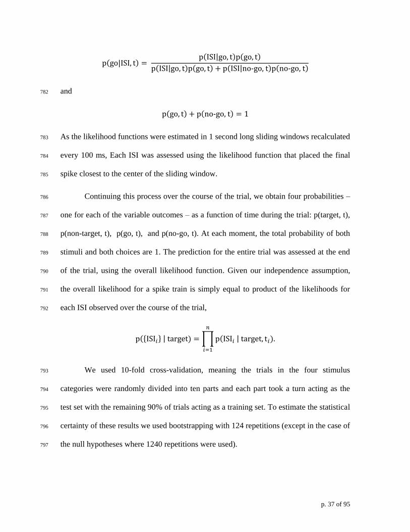
p. 37 of 95

p(go|ISI, t) = p(ISI|go, t)p(go, t)

p(ISI|go, t)p(go, t) + p(ISI|no-go, t)p(no-go, t)

and 782

p(go, t) + p(no-go, t) = 1

As the likelihood functions were estimated in 1 second long sliding windows recalculated 783

every 100 ms, Each ISI was assessed using the likelihood function that placed the final 784

spike closest to the center of the sliding window. 785

Continuing this process over the course of the trial, we obtain four probabilities – 786

one for each of the variable outcomes – as a function of time during the trial: p(target, t), 787

p(non-target, t), p(go, t), and p(no-go, t). At each moment, the total probability of both 788

stimuli and both choices are 1. The prediction for the entire trial was assessed at the end 789

of the trial, using the overall likelihood function. Given our independence assumption, 790

the overall likelihood for a spike train is simply equal to product of the likelihoods for 791

each ISI observed over the course of the trial, 792

p({ISI𝑖} | target) = ∏ p(ISI𝑖 | target, t𝑖)

𝑛

𝑖=1

.

We used 10-fold cross-validation, meaning the trials in the four stimulus 793

categories were randomly divided into ten parts and each part took a turn acting as the 794

test set with the remaining 90% of trials acting as a training set. To estimate the statistical 795

certainty of these results we used bootstrapping with 124 repetitions (except in the case of 796

the null hypotheses where 1240 repetitions were used). 797

p. 38 of 95

Ensemble decoding: Ensemble decoding proceeded very similarly to the single-798

unit case. The ISI probability distributions for each neuron in the ensemble were 799

calculated independently as described above. However, while decoding a given trial, the 800

spike trains of all neurons in the ensemble were used to simultaneously update the beliefs 801

about stimulus category and behavioral choice. In other words, p(stimulus, t) and 802

p(choice, t) were shared for the entire ensemble but each neuron updated them 803

independently using Bayes’ rule whenever a new ISI was encountered. Correlations 804

between neurons were ignored and each of the ISIs from each cell were assumed to were 805

assumed to be independent. For example, if an ISI is observed at time t from neuron j 806

with a likelihood pj: 807

p(target|ISI, t) = p𝑗(ISI|target, t)p(target, t)

p𝑗(ISI|target, t)p(target, t) + p𝑗(ISI|non-target, t)p(non-target, t)

This process is repeated every time a new ISI is encountered from any cell in the 808

ensemble. 809

The joint likelihood of observing a set of ISIs during a trial is then the product of 810

the likelihoods of each neuron independently. For example, for a two neuron ensemble, 811

the combined likelihood, p12, of observing the set {ISI𝑖}1 from neuron 1 and {ISI𝑖}2 from 812

neuron 2 is 813

p12({ISI𝑖}1, {ISI𝑖}2| target) = p1({ISI𝑖}1 | target) p2({ISI𝑖}2 | target)

where pj is the likelihood of observing a given set of ISIs from neuron j. 814

815

Synthetic spike trains 816

p. 39 of 95

To test the null hypothesis that the ISI-based single-trial Bayesian decoder performance 817

was indistinguishable from chance, synthetic spike trains were constructed for each trial 818

of a given unit by randomly sampling with replacement from the set of all observed ISIs 819

regardless of the original task variable values (synthetic spike trains, Figure 4E). In 820

principle under this condition, ISIs should no longer bear any relationship to the task 821

variables and decoding performance should be close to 50%. For single-unit responses, 822

this randomization was completed 1240 times. Significance from the null was assessed 823

by a direct comparison to the 124 bootstrapped values observed from the true data to the 824

1240 values observed under the null hypotheses. The p-value was determined as the 825

probability of finding a value from this synthetic condition that produced better decoding 826

performance than the values actually observed as in a standard permutation test. 827

As a secondary control, we used a traditional permutation test whereby observed 828

spike trains were left intact, but the task variables that correspond to each spike train were 829

randomly permuted (condition permutation, Figure 4F). This process was completed 830

1240 times. 831

832

Rate-modulated Poisson decoding 833

To decode using the trial-averaged firing rate, we implemented a standard method(Rieke 834

et al., 1999) which uses the probability of observing a set of n spikes at times t1, … , tn 835

assuming those spikes were generated by a rate-modulated Poisson process (Figure 4-836

figure supplement 4). Just as with this ISI-based decoder, we decoded activity from the 837

entire trial. First, we use a training set comprising 90% of trials to estimate the time-838

varying firing rate for each condition from the PSTH 839

p. 40 of 95

( 𝑟target(𝑡), 𝑟non-target(𝑡), 𝑟go(𝑡), 𝑟no-go(𝑡)) by Kernel Density Estimation with 10-fold 840

cross-validation. The remaining 10% of spike trains are then decoded using the 841

probability of observing each spike train on each condition assuming they were generated 842

according to a rate-modulated Poisson process 843

p({𝑡𝑖} | target) =1

𝑁!(𝑟target(𝑡1) 𝑟target(𝑡2) … 𝑟target(𝑡𝑛)) exp (− ∫ 𝑟target(𝑡) 𝑑𝑡

𝑇𝑓

𝑇𝑖

) ,

where 𝑇𝑖 and 𝑇𝑓 are the beginning and end of the trial respectively. This likelihood 844

function is straightforward to interpret: the first product is the probability of observing 845

spikes the spikes at the times they were observed (where the 1/N! term serves to divide 846

out by the number of permutations of spike labels) and the exponential term represents 847

the probability of silence in the periods between spikes. For comparison with our method, 848

we can reformulate this equation using interspike intervals, if we first break up the 849

exponential integral into domains that span the observed interspike intervals. 850

p({𝑡𝑖} | target)

=1

𝑁!(𝑟target(𝑡1) exp (− ∫ 𝑟target(𝑡) 𝑑𝑡

𝑡1

𝑇𝑖

))

× (𝑟target(𝑡2) exp (− ∫ 𝑟target(𝑡) 𝑑𝑡𝑡2

𝑡1

)) … × (exp (− ∫ 𝑟target(𝑡) 𝑑𝑡𝑇𝑓

𝑡𝑛

) ).

Collecting the first and last terms relating to trial start and trial end as 851

𝐿𝑖(𝑡1, 𝑇𝑖) ≡ 𝑟target(𝑡1) exp (− ∫ 𝑟target(𝑡) 𝑑𝑡𝑡1

𝑇𝑖

)

𝐿𝑓(𝑡𝑛, 𝑇𝑓) ≡ exp (− ∫ 𝑟target(𝑡) 𝑑𝑡𝑇𝑓

𝑡𝑛

) ,

this becomes 852

p. 41 of 95

p({𝑡𝑖} | target) =1

𝑁!𝐿𝑖 (∏ 𝑟target(𝑡𝑖 + Δ𝑡𝑖)

𝑛−1

𝑖=1

exp (− ∫ 𝑟target(𝑡) 𝑑𝑡𝑡𝑖+Δ𝑡𝑖

𝑡𝑖

)) 𝐿𝑓 ,

where Δti is the time difference between spikes ti and ti+1. The interpretation of each term 853

in the product is straightforward: it is the infinitesimal probability of observing a spike a 854

time Δt after a spike at time t multiplied by the probability of observing no spikes in the 855

intervening time. In other words, it is simply p(ISI | target, 𝑡), the probability of 856

observing an ISI conditioned on observing the first spike at time t, as predicted by the 857

assumption of a rate-modulated Poisson process. We can easily verify that this term is 858

normalized which allows us to write, 859

p(ISI | target, 𝑡) = 𝑟target(𝑡 + ISI) exp (− ∫ 𝑟target(𝑡) 𝑑𝑡𝑡+ISI

𝑡

).

With the exception of the terms relating to trial start and end, we can then view the 860

likelihood of a spike train as resulting from the likelihood of the individual ISIs (just as 861

with our ISI-decoder), 862

p({𝑡𝑖} | target) =1

𝑁!𝐿𝑖 𝐿𝑓 (∏ p(ISI𝑖 | target, 𝑡𝑖)

𝑛−1

𝑖=1

),

with the key difference that these ISI probabilities are inferred from the firing rate rather 863

than estimated directly using non-parametric methods. 864

865

Inferring the ISI distribution predicted by a rate-modulated Poisson process 866

To compare the ISI distribution inferred using non-parametric methods to one predicted 867

by a rate-modulated Poisson process we use the relationship above to calculate the 868

predicted probability of observing an ISI of given length within the 1 second window 869

used for our non-parametric estimates. The formula above assumes a spike has already 870

p. 42 of 95

occurred at time t, so we multiply by the probability of observing a spike at time t, 871

p(𝑡 | target) = 𝑟target(𝑡), to obtain the total probability of finding an ISI at any given 872

point in the trial. 873

p(ISI, 𝑡 | target) = p(ISI | target, t) p(t | target)

= 𝑟target(𝑡) 𝑟target(𝑡 + ISI) exp (− ∫ 𝑟target(𝑡) 𝑑𝑡𝑡+ISI

𝑡

).

In other words, the probability of observing an ISI beginning at time t is simply the 874

probability of observing spikes at times t and t + ISI with silence in between. 875

The probability of observing an ISI at any time within a time window spanning wi 876

to wf is simply the integral of this ISI probability as a function of time across the window. 877

To ensure the final spike occurs before wf the integral spans wi to (wf - ISI), 878

p(ISI | 𝑤𝑖 , 𝑤𝑓 , target) = 𝐶−1 ∫ p(ISI, 𝑡 | target) 𝑑𝑡𝑤𝑓−ISI

𝑤𝑖

where C is a normalization constant which ensures p(ISI | wi, wf, target) integrates to 1, 879

C = ∫ (∫ p(ISI, 𝑡 | target) 𝑑𝑡𝑤𝑓−ISI

𝑤𝑖

) 𝑑ISI𝑤𝑓−𝑤𝑖

0

.

880

Regression based method for verifying multiplexing 881

For each cell, we fit a Logit model for both the stimulus and choice decoding 882

probabilities on individual trials with the true stimulus category and behavioral choice as 883

regressors. We then calculated the extent to which the stimulus decoding probability was 884

determined by true stimulus category by subtracting the regression coefficient for 885

stimulus from that of choice (Figure 4-figure supplement 3A, x-axis, stimulus 886

selectivity index); when this number is positive it indicates that stimulus was a stronger 887

p. 43 of 95

predictor of stimulus decoding on a trial-by-trial basis. The same process was repeated 888

for choice (Figure 4-figure supplement 3A, y-axis, choice selectivity index). According 889

to this analysis we took multiplexed cells to be those that were positive for both measures 890

(Figure 4-figure supplement 3A, orange symbols, 19/90 cells). In other words, 891

multiplexed cells were cells for which stimulus decoding probabilities were primarily a 892

result of true stimulus category and choice decoding probabilities were primarily a result 893

of true behavioral choice. 894

Given the moderate negative correlation for these indices we projected each of 895

these points onto their linear regression to create a one-dimensional regression-based 896

uniplexing index. Cells with a value near zero are the multiplexed cells described above 897

and cells with positive or negative values are primarily stimulus or choice selective 898

(Figure 4-figure supplement 3A). 899

We compared the uniplexing values produced by this regression method to those 900

produced by examining only the average decoding performance for stimulus and choice 901

(Figure 4-figure supplement 3B). A decoding-based uniplexing index was defined as 902

the difference between average stimulus and choice decoding for each cell. When these 903

two values are comparable this measure returns a value close to zero and the cell is 904

considered multiplexed; moreover, cells that are uniplexed for stimulus or choice receive 905

positive and negative values respectively just as with the regression based measure. 906

While the overall magnitude of these two measures need not be related, both measures of 907

multi/uniplexing rank cells on a one-dimensional axis from choice uniplexed to 908

multiplexed to stimulus uniplexed centered on zero. 909

910

p. 44 of 95

911

Weighted log likelihood ratio 912

The log likelihood ratio (LLR) was calculated by first calculating the conditional ISI 913

probabilities and then taking the difference of the logarithm of these distributions. For 914

stimulus, 915

LLRstimulus(ISI) = log2(p(ISI|target)) − log2(p(ISI|non-target)),

and for choice, 916

LLRchoice(ISI) = log2(p(ISI|go)) − log2(p(ISI|no-go)).

The weighted LLR weights the LLR according to the prevalence of a given ISI. For 917

stimulus, 918

W. LLRstimulus(ISI) = p(ISI)[log2(p(ISI|target)) − log2(p(ISI|non-target))],

and for choice, 919

W. LLRchoice(ISI) = p(ISI)[log2(p(ISI|go)) − log2(p(ISI|no-go))].

920

Consensus and unsigned consensus 921

The consensus value evaluates the extent to which the LLR (or weighted LLR) is shared 922

across an ensemble. It is the norm of the sum of the LLRs (W. LLRs) divided by the sum 923

of the norms. In principle, the functional norm can be anything but in this case we used 924

the ℓ1 norm (the absolute area under the curve), 925

‖𝑓‖1 ≡ ∫|𝑓(𝑥)| 𝑑𝑥.

The for an n-member ensemble, the consensus is then 926

Consensus ≡ ‖∑ LLR𝑖

𝑛𝑖=1 ‖1

∑ ‖LLR𝑖‖𝑛𝑖=1 1

.

p. 45 of 95

For the unsigned consensus, we first generate every permutation of the LLRs used and 927

their inverses, -LLR, up to an overall sign. For example, for a pair of LLRs there are only 928

two options, 929

(LLR1, LLR2) or (LLR1, -LLR2), 930

and for three LLRs there are four options, 931

(LLR1, LLR2, LLR3), (-LLR1, LLR2, LLR3), (LLR1, -LLR2, LLR3), 932

or (LLR1, LLR2, -LLR3). 933

The consensus is then calculated over each these sets and the maximum value is taken to 934

be the value of the unsigned consensus. 935

To generate the consensus curves in Figure 8, LLRs are calculated using a 750 936

ms sliding window recalculated every 100 ms. The resulting consensus value is assigned 937

to the center of the 500 ms window. For visual clarity, these values were interpolated by a 938

third-degree univariate spline calculated using the python package 939

scipy.interpolate.InterpolatedUnivariateSpline (this technique is guaranteed to intercept 940

the measured values). 941

942

Analysis of Rodgers & DeWeese 2014 dataset 943

Using our novel ISI-based decoding algorithm, we analyzed cells found to be non-944

classically responsive in a previously published study (Rodgers & DeWeese, 2014). 945

Briefly, rats were trained on a novel auditory stimulus selection task where animals had 946

to respond to one of two cues while ignoring the other depending on the context. Rats 947

held their nose in a center port for 250 to 350 ms and were then presented with two 948

simultaneous sounds (a white noise burst played from only the left or right speaker and a 949

p. 46 of 95

high or low pitched warble played from both speakers). In the “localization” context 950

animals were trained to ignore the warble and respond to the location of the white noise 951

burst and in the “pitch” context they were trained to ignore the location of the white noise 952

burst and respond to the pitch of the warble. Cells recorded from both primary auditory 953

cortex and prefrontal cortex (prelimbic region) were shown to be classically responsive to 954

the selection rule during the pre-stimulus period (i.e. firing rates differed between the two 955

contexts). Non-classically responsive cells were reported but not further analyzed. 956

We established that cells were non-classically responsive for the stimulus location 957

or pitch using our own positive statistical criteria for non-classical responsiveness 958

(described above) by comparing the average spiking activity in the 250 ms stimulus 959

period and the 250 ms following stimulus to inter-trial baseline activity. Cells were also 960

determined to be non-classically responsive for ramping using the same criteria as with 961

our own data. We confirmed that cells were non-classically responsive for the selection 962

rule by comparing their average spiking activity in the 100 ms immediately preceding 963

stimulus onset across contexts. 964

To determine whether non-classically responsive cells also encoded task 965

information (stimulus location, stimulus pitch, behavioral choice, and the selection rule), 966

we decoded each variable on single-trials using our ISI-based decoding algorithm. 967

Selection rule information was only assessed in the pre-stimulus hold period whereas 968

stimulus and choice information was assessed in the period after stimulus onset prior to 969

behavioral response (as with our own data). Cells shown in Figure 5B were deemed 970

statistically significant when compared to the decoding performance of a control using 971

synthetically generated data (p<0.05). 972

p. 47 of 95

973

Statistical analysis 974

All statistical analyses were performed in Python, MATLAB, or GraphPad Prism 6. 975

Datasets were tested for normality, and appropriate statistical tests applied as described in 976

the text (e.g., Student’s paired t-test for normally distributed data, Mann-Whitney U test 977

for unmatched non-parametric data, and Wilcoxon matched-pairs signed rank test for 978

matched non-parametric data). 979

p. 48 of 95

980

Code and sample data availability: https://github.com/badralbanna/Insanally2017 981

982

Acknowledgements: We thank E. Simoncelli, N.D. Daw, C.S. Peskin, A.A. Fenton, E. 983

Kelemen, K. Kuchibhotla, E. Morina, M. Aoi, and A. Charles for comments, discussions, 984

and technical assistance, and C.A. Loomis and the NYU School of Medicine Histology 985

Core for assistance with anatomical studies. Shari E. Ross produced the illustration in 986

Figure 1A. This work was funded by an NYU Provost’s Postdoctoral Fellowship and 987

NIDCD (DC015543-01A1) to M.N.I.; a NARSAD Young Investigators Award, NIMH 988

(T32), and NIMH (KMH106744A) to I.C.; a James McDonnell Understanding Human 989

Cognition Scholar Award to K.R; a Fordham University Grant for Cloud Based 990

Computing Research Projects to B.F.A.; and NIDCD (DC009635 and DC012557), the 991

NYU Grand Challenge Award, a Howard Hughes Medical Institute Faculty Scholarship, 992

a Hirschl/Weill-Caulier Career Award, and a Sloan Research Fellowship to R.C.F. The 993

authors declare no competing financial interests. 994

995

Competing Interests: The authors declare no competing financial interests. 996

Correspondence and requests for materials should be addressed to 997

robert.froemke@med.nyu.edu. 998

999

1000

1001

1002

p. 49 of 95

References 1003

Carcea, I., Insanally, M. N., & Froemke, R. C. (2017). Dynamics of auditory cortical activity during 1004

behavioural engagement and auditory perception. Nature Communications, 8, 14412. 1005

https://doi.org/10.1038/ncomms14412 1006

Churchland, A. K., Kiani, R., & Shadlen, M. N. (2008). Decision-making with multiple alternatives. Nature 1007

Neuroscience, 11(6), 693–702. https://doi.org/10.1038/nn.2123 1008

David, S. V., Fritz, J. B., & Shamma, S. A. (2012). Task reward structure shapes rapid receptive field 1009

plasticity in auditory cortex. Proceedings of the National Academy of Sciences, 109(6), 2144–1010

2149. https://doi.org/10.1073/pnas.1117717109 1011

DeWeese, M. R., Wehr, M., & Zador, A. M. (2003). Binary spiking in auditory cortex. The Journal of 1012

Neuroscience, 23(21), 7940–7949. 1013

Erlich, J. C., Bialek, M., & Brody, C. D. (2011). A cortical substrate for memory-guided orienting in the 1014

rat. Neuron, 72(2), 330–343. https://doi.org/10.1016/j.neuron.2011.07.010 1015

Fritz, J. B., David, S. V., Radtke-Schuller, S., Yin, P., & Shamma, S. A. (2010). Adaptive, behaviorally 1016

gated, persistent encoding of task-relevant auditory information in ferret frontal cortex. Nature 1017

Neuroscience, 13(8), 1011–1019. https://doi.org/10.1038/nn.2598 1018

Fritz, J., Shamma, S., Elhilali, M., & Klein, D. (2003). Rapid task-related plasticity of spectrotemporal 1019

receptive fields in primary auditory cortex. Nature Neuroscience, 6(11), 1216–1223. 1020

https://doi.org/10.1038/nn1141 1021

Froemke, R. C., Carcea, I., Barker, A. J., Yuan, K., Seybold, B. A., Martins, A. R. O., … Schreiner, C. E. 1022

(2013). Long-term modification of cortical synapses improves sensory perception. Nature 1023

Neuroscience, 16(1), 79–88. https://doi.org/10.1038/nn.3274 1024

Gimenez, T. L., Lorenc, M., & Jaramillo, S. (2015). Adaptive categorization of sound frequency does not 1025

require the auditory cortex in rats. Journal of Neurophysiology, 114(2), 1137–1145. 1026

https://doi.org/10/f7p5bm 1027

Hangya, B., Ranade, S. P., Lorenc, M., & Kepecs, A. (2015). Central cholinergic neurons are rapidly 1028

recruited by reinforcement feedback. Cell, 162(5), 1155–1168. 1029

https://doi.org/10.1016/j.cell.2015.07.057 1030

p. 50 of 95

Hanks, T. D., Kopec, C. D., Brunton, B. W., Duan, C. A., Erlich, J. C., & Brody, C. D. (2015). Distinct 1031

relationships of parietal and prefrontal cortices to evidence accumulation. Nature, 520(7546), 220–1032

223. https://doi.org/10.1038/nature14066 1033

Hromádka, T., DeWeese, M. R., Zador, A. M., & others. (2008). Sparse representation of sounds in the 1034

unanesthetized auditory cortex. PLoS Biol, 6(1), e16. 1035

Hubel, D. H., Henson, C. O., Rupert, A., & Galambos, R. (1959). “Attention” units in the auditory cortex. 1036

Science, 129(3358), 1279–1280. 1037

Izhikevich, E. (2000). Neural excitability, spiking and bursting. International Journal of Bifurcation and 1038

Chaos, 10(6), 1171–1266. 1039

Jaramillo, S., Borges, K., & Zador, A. M. (2014). Auditory thalamus and auditory cortex are equally 1040

modulated by context during flexible categorization of sounds. The Journal of Neuroscience, 1041

34(15), 5291–5301. https://doi.org/10.1523/JNEUROSCI.4888-13.2014 1042

Jaramillo, S., & Zador, A. M. (2010). The auditory cortex mediates the perceptual effects of acoustic 1043

temporal expectation. Nature Neuroscience, 14(2), 246–251. 1044

Jones, M. C., Marron, J. S., & Sheather, S. J. (1996). A brief survey of bandwidth selection for density 1045

estimation. Journal of the American Statistical Association, 91(433), 401–407. 1046

https://doi.org/10.1080/01621459.1996.10476701 1047

Kadia, S. C., & Wang, X. (2002). Spectral integration in A1 of awake primates: neurons with single and 1048

multipeaked tuning characteristics. Journal of Neurophysiology, 89(3), 1603–1622. 1049

https://doi.org/10.1152/jn.00271.2001 1050

Kiani, R., & Shadlen, M. N. (2009). Representation of confidence associated with a decision by neurons in 1051

the parietal cortex. Science, 324(5928), 759–764. https://doi.org/10.1126/science.1169405 1052

King, J., Shehu, I., Roland, J. T., Svirsky, M. A., & Froemke, R. C. (2016). A physiological and behavioral 1053

system for hearing restoration with cochlear implants. Journal of Neurophysiology, 116(2), 844–1054

858. https://doi.org/10.1152/jn.00048.2016 1055

Kuchibhotla, K. V., Gill, J. V., Lindsay, G. W., Papadoyannis, E. S., Field, R. E., Sten, T. A. H., … 1056

Froemke, R. C. (2017). Parallel processing by cortical inhibition enables context-dependent 1057

behavior. Nature Neuroscience, 20(1), 62–71. https://doi.org/10.1038/nn.4436 1058

p. 51 of 95

Leavitt, M. L., Pieper, F., Sachs, A. J., & Martinez-Trujillo, J. C. (2017). Correlated variability modifies 1059

working memory fidelity in primate prefrontal neuronal ensembles. Proceedings of the National 1060

Academy of Sciences, 114(12), E2494–E2503. https://doi.org/10/f9wt5h 1061

Lu, T., & Wang, X. (2004). Information content of auditory cortical responses to time-varying acoustic 1062

stimuli. Journal of Neurophysiology, 91(1), 301–313. https://doi.org/10.1152/jn.00022.2003 1063

Lundstrom, B. N., & Fairhall, A. L. (2006). Decoding stimulus variance from a distributional neural code 1064

of interspike intervals. Journal of Neuroscience, 26(35), 9030–9037. 1065

https://doi.org/10.1523/JNEUROSCI.0225-06.2006 1066

Markram, H., & Tsodyks, M. (1996). Redistribution of synaptic efficacy between neocortical pyramidal 1067

neurons. Nature, 382(6594), 807–810. https://doi.org/10/bjwc9g 1068

Martins, A. R. O., & Froemke, R. C. (2015). Coordinated forms of noradrenergic plasticity in the locus 1069

coeruleus and primary auditory cortex. Nature Neuroscience, 18(10), 1483–1492. 1070

https://doi.org/10.1038/nn.4090 1071

Merzenich, M. M., Knight, P. L., & Roth, G. L. (1975). Representation of cochlea within primary auditory 1072

cortex in the cat. Journal of Neurophysiology, 38(2), 231–249. 1073

Murakami, M., Vicente, M. I., Costa, G. M., & Mainen, Z. F. (2014). Neural antecedents of self-initiated 1074

actions in secondary motor cortex. Nature Neuroscience, 17(11), 1574–1582. 1075

https://doi.org/10.1038/nn.3826 1076

Olshausen, B. A., & Field, D. J. (2006). What is the other 85% of V1 doing? In T. J. Sejnowski & L. van 1077

Hemmen (Eds.), 23 Problems in Systems Neuroscience (pp. 182–221). Oxford University Press. 1078

Otazu, G. H., Tai, L.-H., Yang, Y., & Zador, A. M. (2009). Engaging in an auditory task suppresses 1079

responses in auditory cortex. Nature Neuroscience, 12(5), 646–654. 1080

https://doi.org/10.1038/nn.2306 1081

Polley, D. B., Read, H. L., Storace, D. A., & Merzenich, M. M. (2007). Multiparametric auditory receptive 1082

field organization across five cortical fields in the albino rat. Journal of Neurophysiology, 97(5), 1083

3621–3638. https://doi.org/10.1152/jn.01298.2006 1084

p. 52 of 95

Raposo, D., Kaufman, M. T., & Churchland, A. K. (2014). A category-free neural population supports 1085

evolving demands during decision-making. Nature Neuroscience, 17(12), 1784–1792. 1086

https://doi.org/10.1038/nn.3865 1087

Reich, D. S., Mechler, F., Purpura, K. P., & Victor, J. D. (2000). Interspike intervals, receptive fields, and 1088

information encoding in primary visual cortex. The Journal of Neuroscience: The Official Journal 1089

of the Society for Neuroscience, 20(5), 1964–1974. 1090

Rieke, F., Warland, D., de de Ruyter van Steveninck, R., & Bialek, W. (1999). Spikes: Exploring the 1091

Neural Code. A Bradford Book. 1092

Rigotti, M., Barak, O., Warden, M. R., Wang, X.-J., Daw, N. D., Miller, E. K., & Fusi, S. (2013). The 1093

importance of mixed selectivity in complex cognitive tasks. Nature, 497(7451), 585–590. 1094

https://doi.org/10.1038/nature12160 1095

Rodgers, C. C., & DeWeese, M. R. (2014). Neural correlates of task switching in prefrontal cortex and 1096

primary auditory cortex in a novel stimulus selection task for rodents. Neuron, 82(5), 1157–1170. 1097

https://doi.org/10.1016/j.neuron.2014.04.031 1098

Romanski, L. M., Bates, J. F., & Goldman-Rakic, P. S. (1999). Auditory belt and parabelt projections to the 1099

prefrontal cortex in the rhesus monkey. The Journal of Comparative Neurology, 403(2), 141–157. 1100

Schneider, D. M., Nelson, A., & Mooney, R. (2014). A synaptic and circuit basis for corollary discharge in 1101

the auditory cortex. Nature, 513(7517), 189–194. https://doi.org/10.1038/nature13724 1102

Wehr, M., & Zador, A. M. (2003). Balanced inhibition underlies tuning and sharpens spike timing in 1103

auditory cortex. Nature, 426(6965), 442–446. https://doi.org/10.1038/nature02116 1104

Weinberger, N. M. (2007). Auditory associative memory and representational plasticity in the primary 1105

auditory cortex. Hearing Research, 229(1–2), 54–68. https://doi.org/10.1016/j.heares.2007.01.004 1106

Wiener, M. C., & Richmond, B. J. (2003). Decoding spike trains instant by instant using order statistics and 1107

the mixture-of-Poissons model. The Journal of Neuroscience, 23(6), 2394–2406. 1108

Yaron, A., Hershenhoren, I., & Nelken, I. (2012). Sensitivity to complex statistical regularities in rat 1109

auditory cortex. Neuron, 76(3), 603–615. https://doi.org/10.1016/j.neuron.2012.08.025 1110

p. 53 of 95

Zuo, Y., Safaai, H., Notaro, G., Mazzoni, A., Panzeri, S., & Diamond, M. E. (2015). Complementary 1111

Contributions of Spike Timing and Spike Rate to Perceptual Decisions in Rat S1 and S2 Cortex. 1112

Current Biology, 25(3), 357–363. https://doi.org/10.1016/j.cub.2014.11.065 1113

Zylberberg, J. (2018). The Role of Untuned Neurons In Sensory Information Coding. BioRxiv, 134379. 1114

https://doi.org/10/gfppmj 1115

1116

1117

p. 54 of 95

1118

1119

Figure 1. Recording from AC or FR2 during go/no-go audiomotor task. (A) 1120

Behavioral schematic for the go/no-go frequency recognition task. Animals were 1121

rewarded with food for entering the nose port within 2.5 seconds after presentation of a 1122

target tone (4 kHz) or given a 7- second time-out if they incorrectly responded to non-1123

target tones (0.5, 1, 2, 8,16, or 32 kHz). (B) Behavioral responses (nose pokes) to target 1124

and non-target tones (hit rates: 88 ± 7%, false alarms: 7 ± 5%, N=15 rats). (C) Left, AC 1125

p. 55 of 95

unit with significant tone modulated responses during target trials (red; top panel, average 1126

evoked spikes = 0.55) and non-target trials (blue; bottom panel, average evoked spikes = 1127

0.92). Rasters of individual trials as well as the firing rate histogram and moving average 1128

are shown. Histograms of average firing rate during a trial were constructed using 25 ms 1129

time bins. A moving average of the firing rate was constructed using a Gaussian kernel 1130

with a 20 ms standard deviation. Black circles represent behavioral responses. Right, 1131

population averages for all target (n=23) or nontarget (n=34) classically responsive singe-1132

units from AC. (D) Left, FR2 unit with ramping activity (green; ramp index = 2.82). 1133

Trials here are aligned to response time. Diamonds indicate stimulus onset. Right, 1134

population average for all ramping single-units from FR2 (n=21). (E) Left, FR2 unit that 1135

was not significantly modulated during target trials (red; average evoked spikes = .041, 1136

p<.001, 2,000 bootstraps). Black circles here represent behavioral responses. Right, 1137

population averages for all target (n=44) or non-target (n=44) non-classically responsive 1138

single-units from FR2 (F) Left, FR2 unit lacking ramping activity (green, ramp index = -1139

1.0, p<.001, 2,000 bootstraps). Right, population average for all non-ramping single-units 1140

from FR2 (n=44). 1141

p. 56 of 95

1142

Figure 2. ISIs capture information distinct from trial-averaged rate. Three simulated 1143

example neurons demonstrating that differences in the ISI are not necessary for 1144

differences in the trial-averaged firing rate to occur (and vice versa). Each trial was 1145

generated by randomly sampling from the appropriate conditional ISI distribution. 1146

Evoked responses were generated by shifting trials without altering the ISI distributions 1147

such that one spike during stimulus presentation is found at approximately 30 ms (with a 1148

p. 57 of 95

variance of 10 ms). (A) Example neuron with both an evoked target response and a 1149

difference in the conditional ISI distributions on target and non-target trials. (B) Example 1150

neuron with an evoked target response but identical conditional ISI distributions. 1151

(C) Example non-classically responsive neuron with no distinct trial-averaged activity 1152

relative to the pre-stimulus period that nevertheless is generated by distinct ISI 1153

distributions. 1154

1155

Source data has been provided in the spreadsheet titled ‘figure_2.csv’. 1156

p. 58 of 95

1157

Figure 3. ISI-based algorithm for decoding behavioral variables from AC and FR2 1158

single-units. (A) Single-unit activity was first sorted by task condition, here for target 1159

trials (red) and non-target trials (blue). All ISIs following stimulus onset and before 1160

behavioral choice were aggregated into libraries for each condition (average response 1161

time is used on no-go trials) as shown for a sample trial. (B) Probability of observing a 1162

given ISI on each condition was generated via Kernel Density Estimation on libraries 1163

from (A). Left, target (red) and non-target (blue) probabilities. Right, go (green) and no-1164

go (purple). (C) Relative differences between the two stimulus conditions (or choice 1165

conditions) was used to infer the actual stimulus category (or choice) from an observed 1166

spike train, in terms of weighted log likelihood ratio (W. LLR) for stimulus category 1167

(p(ISI)*(log2p(ISI|target) - log2(ISI|non-target)); on left) and behavioral choice 1168

(p(ISI)*(log p2(ISI|go) - log2(ISI|no-go)); on right). When curve is above zero the ISI 1169

suggests target (go) and when below zero the ISI suggests non-target (no-go). (D) 1170

p. 59 of 95

Probability functions from c were used as the likelihood function to estimate the 1171

prediction of a spike train on an individual trial (bottom). Bayes’ rule was used to update 1172

the probability of a stimulus (top) or choice (bottom) as the trial progressed and more 1173

ISIs were observed. The prediction for the trial was assessed at the end of the trial. 1174

p. 60 of 95

1175

Figure 4. Decoding performance of single-units recorded from AC or FR2. (A) 1176

Decoding performance of single-units for stimulus category and behavioral choice in AC 1177

(open circles) and FR2 (filled circles) restricted to those statistically significant relative to 1178

synthetically-generated spike trains (p<0.05, permutation test, two-sided). Note that 1179

decoding performance values reflect the algorithm’s prediction certainty on individual 1180

trials. Central symbol with error bars represents group medians and top and bottom 1181

quartiles (*p=0.02, **p=0.001, Mann-Whitney U test, two-sided). Black symbols, 1182

classically responsive cells; red symbols, non-classically responsive cells. (B) Decoding 1183

performance for choice versus stimulus, restricted to those statistically significant relative 1184

to synthetically-generated spike trains for either stimulus, choice, or both (p<0.05, 1185

permutation test, two-sided). Black symbols, classically responsive cells; red symbols, 1186

p. 61 of 95

non-classically responsive cells. (C) Choice decoding performance in AC of non-1187

classically responsive cells (red) and choice non-classically responsive (dark-red) versus 1188

choice classically responsive cells (black; i.e. ramping cells). Decoding performance was 1189

not statistically different (p=0.32 Mann-Whitney U test, two-sided). Central symbol with 1190

error bars represents group medians and top and bottom quartiles. (D) Stimulus decoding 1191

performance in FR2 for non-classically responsive cells (red) and sensory non-classically 1192

responsive (dark-red) versus choice responsive cells (black; i.e. ramping cells). Decoding 1193

performance was not statistically different (p=0.29, Mann-Whitney U test, two-sided). 1194

Central symbol with error bars represents group medians and top and bottom quartiles. 1195

(E) Decoding performance for choice versus stimulus, applied to spike trains 1196

synthetically generated from sampling (with replacement) over all ISIs observed without 1197

regard to stimulus category or behavioral choice. Black, classically responsive cells; red, 1198

non-classically responsive cells. Error bars represent standard deviation. (F) Decoding 1199

performance for choice versus stimulus, applied to spike trains left intact but trial 1200

conditions (stimulus category and behavioral choice) were randomly permuted (1000 1201

permutations per unit). Error bars represent standard deviation. 1202

1203

p. 62 of 95

1204

Figure 5. Information captured by ISI-based decoder distinct from conventional 1205

rate-modulated (inhomogeneous) Poisson decoder. (A) Decoding performance 1206

p. 63 of 95

comparison for example neurons shown in Figure 2. Left, Both the trial-averaged firing 1207

rate and the ISI distributions can be used to decode stimulus category for this example 1208

neuron. Middle, Only the firing rate can be used to decode this example. Right, In this 1209

case, the ISI distributions can be used to decode even when the trial-averaged firing rate 1210

cannot. (B) Comparison of decoding performance for conventional rate-modulated 1211

decoder to our ISI-based decoder. Top row, stimulus decoding, bottom row, choice 1212

decoding. Left, Overall comparison for all cells. Right, Comparison for classically 1213

responsive and non-classically responsive cells (Stimulus Overall: ***pAC=0.0001, 1214

***pFR2=8×10-6

, Stimulus Repsonsive: *pAC=0.031, ***pFR2=4×10-5

, Stimulus non-1215

classically responsive: **pAC=0.0019, n.s. pFR2=0.096, Choice Overall: **pAC=0.0057, 1216

*pFR2=0.02, Choice Repsonsive: n.s. pAC=0.031, n.s. pFR2=0.08, Choice non-classically 1217

responsive: *pAC=0.004, n.s. pFR2=0.19, Wilcoxon signed-rank test). Individual cells 1218

shown and median with error bars designating bottom and top quartiles superimposed. 1219

(C) Left, Matthews correlation coefficient (MCC) between correct predictions of our ISI-1220

based decoder and a conventional rate-modulated firing rate decoder. A MCC value of 1 1221

indicates each decoder correctly decodes exactly the same set of trials whereas -1 1222

indicates each decoder is correct on complementary trials. Values close to 0 indicate that 1223

that the relationship between the decoders is close to chance. Typically, values from -0.5 1224

to 0.5 are considered evidence for weak to no correlation (stimulus median & 1225

interquartile range: AC=0.10, 0.09, FR2=0.11, 0.12; choice median & interquartile range: 1226

AC=0.06, 0.15, FR2=0.08, 0.17). Right, Matthews correlation coefficient (MCC) 1227

rescaled by the maximum possible correlation given the decoding performance of each 1228

method remains fixed. This control demonstrates that the correlation values are not a 1229

p. 64 of 95

result of weak decoding performance for one of the decoding methods (stimulus median 1230

& interquartile range: AC=0.11, 0.11, FR2=0.12, 0.15; choice median & interquartile 1231

range: AC=0.08, 0.17, FR2=0.11, 0.19). 1232

1233

Source data has been provided in the spreadsheet titled ‘figure_5.csv’. 1234

1235

p. 65 of 95

1236

Figure 6. Non-classically responsive cells in both auditory cortex and prefrontal 1237

cortex (PFC) encode behavioral variables including the selection rule in a task 1238

switching paradigm. (A) Schematic of novel auditory stimulus selection task. Animals 1239

were presented with two simultaneous tones (a white noise burst and warble) and trained 1240

to respond to the location of the sound in the “localization” context while ignoring pitch 1241

and respond to the pitch while ignoring the location in the “pitch” context (figure adapted 1242

from Rodgers & DeWeese 2014, Neuron). Decoding performance for (B) stimulus 1243

localization on localization trials (pAC=0.24, pPFC=0.21, Mann-Whitney U test, two-1244

sided), (C) stimulus pitch on pitch trials (pAC=0.48, pPFC=0.47, Mann-Whitney U test, 1245

two-sided), and (D) choice (**pAC=0.0064, pPFC=0.22, Mann-Whitney U test, two-sided) 1246

for classically responsive cells (black) and non-classically responsive cells (red; no 1247

p. 66 of 95

stimulus modulation or ramping activity) in auditory (open symbols) and prefrontal 1248

cortex (closed symbols) previously reported but not further analyzed in this study. (E) 1249

Decoding performance for the selection rule for classically responsive (black) and non-1250

classically responsive cells (red; similar pre-stimulus firing rates for both pitch and 1251

localization blocks; ***pAC=5×10-6

, ***pPFC<0.0002, Mann-Whitney U test, two-sided). 1252

p. 67 of 95

1253

Figure 7. Decoding performance of neuronal ensembles recorded in AC or FR2. (A) 1254

Schematic of ensemble decoding. Left, conditional ISI distributions and corresponding 1255

weighted LLR shown for two simultaneously recorded neurons. Right, an example trial 1256

where each neuron’s ISIs and LLRs are used to independently update stimulus category 1257

according to Bayes’ rule. Arrows indicate the first updates from each neuron. (B) 1258

Stimulus and choice decoding performance for ensembles in AC and FR2 for ensembles 1259

of increasing size (Comparing smallest with largest ensembles. Stimulus: *pAC=0.04, 1260

***pFR2=1×10-5

, Choice: pAC=0.29, ***pFR2=7×10-5

, Mann-Whitney U test, two-sided). 1261

p. 68 of 95

(C) Error prediction performance in AC and FR2 as a function of ensemble size 1262

(*pAC=0.03, **pFR2=0.002; comparison between AC and FR2, for 3-member ensembles: 1263

p=1.2×10-5

, for 4-member ensembles: p=0.03, Mann-Whitney U test, two-sided). Chance 1264

performance is 50%. (D) Error prediction performance in AC and FR2 as a function of 1265

the number of non-classically responsive cells in the ensemble (*pAC=0.037, Welch’s t-1266

test with Bonferroni correction for multiple comparisons; *pFR2=0.015, Student’s t-test 1267

with Bonferroni correction), 3 and 5 member ensembles in c. shown for AC and FR2 1268

respectively. Chance performance is 50%. 1269

p. 69 of 95

1270

Figure 8. Ensemble consensus-building during behavior. (A) Schematic of consensus 1271

building in a three-member ensemble. When the LLRs of ensemble members are similar 1272

the meaning of any ISI is unambiguous to a downstream neuron. (B) Schematic of a 1273

three-member ensemble without consensus. The meaning of an ISI depends on the 1274

p. 70 of 95

upstream neuron it originates from. (C) ISI distributions, and LLRs for three members of 1275

a sample ensemble. Note that despite differences in ISI distributions, neuron #1 and 1276

neuron #2 have similar weighted log-likelihood ratios (ISIs > 200 ms indicate target, ISIs 1277

< 200 ms indicate non-target). (D) Consensus values for three illustrative two-member 1278

ensembles. Ensemble 1 members have identical LLRs, agreeing on the meaning of all 1279

ISIs (consensus = 1) and on how the ISIs should be partitioned (unsigned consensus = 1). 1280

Ensemble 2 contains cells with LLRs where the ISI meanings are reversed, disagreeing 1281

on meaning of the ISIs (consensus = 0) but still agree on how the ISIs should be 1282

partitioned (unsigned consensus = 1). Ensemble 3 contains two cells with moderate 1283

agreement about the ISI meanings and partitioning, leading to intermediate consensus and 1284

unsigned consensus values (0.5 for each). (E) Left, mean consensus as a function of time 1285

from tone onset (stimulus-aligned) on correct trials for three-member sensory classically 1286

responsive ensembles in AC (two or more members sensory classically responsive; black 1287

dotted line; n=11 ensembles) and sensory non-classically responsive ensembles in FR2 1288

(two or more members sensory non-classically responsive; dark red solid line; n=101 1289

ensembles). Standard deviation shown around each mean trendline. Thin solid and dotted 1290

line represent an individual consensus trajectory from FR2 and AC respectively. FR2 1291

sensory non-classically responsive cells consistently reached consensus and then 1292

diverged immediately after stimulus presentation (consensus, t = 0 to 0.42 s, pSNR = 1293

3.9×10-4

Wilcoxon test with Bonferroni correction, two-sided). AC classically responsive 1294

ensembles (black) increase consensus until 750 ms (Δconsensus, t = 0 to 0.81 s, pSR = 1295

0.14 Wilcoxon test with Bonferroni correction, two-sided). Right, mean consensus as a 1296

function of time to behavioral response (response-aligned) on correct trials for three-1297

p. 71 of 95

member choice classically responsive ensembles (two or more members choice 1298

classically responsive; black) in FR2 (solid line; n=47 ensembles) and choice non-1299

classically responsive (two or more members choice non-classically responsive; dark red) 1300

in AC (dotted line; n=11 ensembles) and FR2 (solid line; n=57 ensembles). Standard 1301

deviation shown around each mean trendline. On correct trials, choice classically 1302

responsive (black) and choice non-classically responsive ensembles (dark red) in both 1303

regions reached high consensus values ~500 ms before response (Δconsensus, t = -1.0 to 1304

0.0 s, pCNR = 2.0×10-5

, pCR = 0.12 Wilcoxon test with Bonferroni correction, two-sided). 1305

(F) As in e, but for error trials (Δconsensus, correct vs. error trials, stimulus: pSNR= 0.007, 1306

pSR = 0.065, choice: pCNR = 0.0048, pCR = 0.065 Mann-Whitney U test, two-sided). (G) 1307

Unsigned consensus index for non-classically responsive ensembles (two or more 1308

members non-classically responsive) in AC (dotted line; n=13 ensembles) and FR2 (solid 1309

line; n=36 ensembles), stimulus-aligned (left, Δconsensus, t = 0 to 0.89 s, p = 5.1×10-5

1310

Wilcoxon test with Bonferroni correction, two-sided) and response-aligned (right, 1311

Δconsensus, t = -1.0 to 0.0 s, p = 0.0033 Wilcoxon test with Bonferroni correction, two-1312

sided). On correct trials, ensembles reach high values of unsigned consensus ~750 ms 1313

after tone onset and within 500 ms of behavioral response. (H) As in (G), but for error 1314

trials (Δconsensus, correct vs. error trials, p = 1.9×10-9

Mann-Whitney U test, two-sided). 1315

(E) – (G) Combinations analyzed and shown are those for which there are significant 1316

numbers in our dataset. 1317

p. 72 of 95

Supplementary Figures 1318

1319

p. 73 of 95

Figure 1-figure supplement 1. Individual response curves from 15 animals included 1320

in this study. Each panel shows data from a different animal including behavioral d' for 1321

distinguishing target from non-target tones. We used a criteria of d' ≥1 for inclusion in 1322

this study. Response curves here are for an average of 3-4 sessions. Error bars represent 1323

S.E.M. 1324

p. 74 of 95

1325

Figure 1-figure supplement 2. Histological placement of cannulas in AC and FR2. 1326

(A) Example of a coronal section of a rat implanted with cannulas in primary auditory 1327

cortex (AC). The white lines represent the borders of AC38

. (B) Example of a coronal 1328

section of a rat implanted with cannulas in FR2. The white lines represent the borders of 1329

FR238

. 1330

p. 75 of 95

1331

Figure 1-figure supplement 3. Bilateral infusion of muscimol into either AC or FR2 1332

significantly impairs task performance. (A) Behavioral performance after muscimol 1333

infusion (red) or saline control (black) in AC from two individual animals. (B) Summary 1334

of performance on day before infusion, after muscimol infusion into AC, and after saline 1335

control infusion (N=3 animals). Performance was impaired after muscimol infusion 1336

(p=0.03 Student’s paired two-tailed t-test, *p <0.05). (C) Behavior of one animal allowed 1337

to freely nose poke for food without tones being presented. This behavior was not 1338

affected by muscimol inactivation (average of 3 sessions, p>0.99 Wilcoxon matched-1339

pairs signed rank test). Error bars represent S.E.M. (D) Behavioral performance for two 1340

animals infused bilaterally with muscimol into FR2. (E) Summary of performance before, 1341

during, and after muscimol infusion into FR2 (N=5 animals). Performance was impaired 1342

after muscimol infusion (p=0.009 Student’s paired two-tailed t-test, **p<0.01). (F) 1343

Muscimol in FR2 did not impair free nose poking for food without tones being presented 1344

in two animals (average of 4 sessions, p=0.62, Wilcoxon matched-pairs signed rank test). 1345

p. 76 of 95

1346

Figure 1-figure supplement 4. Histological placement of electrodes in AC and FR2. 1347

(A) Example of electrode tracks and electrolytic lesions in AC. The white lines represent 1348

the borders of AC. (B) Example of an electrode track in FR2. The white lines represent 1349

the borders of FR2. Left, section imaged at 10X. Right, the same section imaged at 40X. 1350

p. 77 of 95

1351

Figure 1-figure supplement 5. Examples of tone evoked, ramping, and non-1352

classically responsive cells from AC and FR2. (A) Two example tone-evoked cells 1353

recorded from AC. Rasters and PSTHs of target (red) and non-target (blue) trials shown. 1354

p. 78 of 95

Stimulus shown as grey bar and black circles represent behavioral response. (Example 1355

#1: average evoked spikes on target tones = 0.55, on non-target = 0.92. Example #2: 1356

average evoked spikes on target tones = 0.096, on non-target = 0.12; note that example 1357

#2 is only non-target tone evoked). (B) Example target tone-evoked cell recorded from 1358

FR2. Rasters and PSTHs of target (red) and non-target (blue) trials shown (average 1359

evoked spikes on target tones = 0.37, on non-target = 0.20). (C) Example ramping cell 1360

recorded from AC. Rasters and PSTH of go trials (green) shown (ramp index = 2.8). (D) 1361

Example ramping cell recorded from FR2 (ramp index = 4.9). Rasters and PSTH of go 1362

trials (green) shown. (E) Two example non-classically responsive cells recorded from 1363

AC. Rasters and PSTH of target (red), non-target (blue), and go (green) trials shown. 1364

(Example #1: average evoked spikes on target tones = 0.12, on non-target = -0.12, ramp 1365

index = -0.85; ptone<0.001, pramp=0.010, 2,000 bootstraps; Example #2: average evoked 1366

spikes on target tones = -0.020, on non-target = -0.038, ramp index = 1.1; ptone<0.001, 1367

pramp=0.004, 2,000 bootstraps). (F) Two example non-classically responsive cells 1368

recorded from FR2 (Example #1: average evoked spikes on target tones = 0.081, on non-1369

target = -0.15, ramp index = 1.4; ptone<0.001, pramp=0.019, 2,000 bootstraps; Example #2: 1370

average evoked spikes on target tones = 0.046, on non-target = -0.070, ramp index = 1.8; 1371

ptone<0.001, pramp=0.033, 2,000 bootstraps). Rasters and PSTH of target (red), non-target 1372

(blue), and go (green) trials shown. 1373

p. 79 of 95

1374

Figure 1-figure supplement 6. Summary statistics. Histograms of (A) spontaneous 1375

firing rate, (B) average number of tone-evoked spikes for preferred stimulus category, 1376

and (C) ramp index for AC (top) and FR2 (bottom). 1377

p. 80 of 95

1378

Figure 3-figure supplement 1. Decoding algorithm to determine stimulus category 1379

p. 81 of 95

and choice in single-unit ISIs from AC and FR2 for two additional neurons. (A-D) 1380

Decoding algorithm applied to a sample neuron in AC. (A) Single-unit activity sorted by 1381

stimulus condition: target trials (red) and non-target trials (blue). Black circles represent 1382

the behavioral response. (B) Trials aligned to behavioral response: go (green) and no-go 1383

(purple). Black diamonds in both go and no-go trials represent stimulus onset. (C) All 1384

ISIs during the trial (following stimulus onset and before behavioral choice) are 1385

aggregated into libraries for each condition (average response time is used on no-go 1386

trials). Probability of observing a given ISI on each condition was generated by using 1387

Kernel Density Estimation on the libraries from (A). Top left are target (red) and non-1388

target (blue) probabilities and on right are go (green) and no-go (purple). Below left 1389

(right) are the log likelihood ratios (LLR) for the ISIs conditioned on stimulus category 1390

(behavioral choice). When curve is above zero the ISI suggests target (go); when it is 1391

below zero the ISI suggests non-target (no-go). (D) Probability functions from c. were 1392

used as the likelihood function to estimate the prediction of a spike train on an individual 1393

trial (bottom). Bayes’ rule was used to update the probability of a stimulus (top) or choice 1394

(bottom) as the trial progresses and more ISIs were observed. Prediction for the trial was 1395

assessed at the end of the trial as depicted by the highlighted dot. (E-H) as in (A-D) 1396

except the decoding algorithm is applied to a neuron from FR2. 1397

p. 82 of 95

1398

1399

Figure 3-figure supplement 2. Empirical ISI distributions are better modeled using 1400

non-parametric methods. (A) ISI histograms from two example cells on target trials 1401

with the corresponding non-parametric Kernel Density Estimate (KDE) distribution 1402

(solid lines) and the distribution derived from a rate-modulated Poisson process (dashed 1403

lines). Above each example is the Kullback-Leibler divergence (DKL) quantifying the 1404

difference between these two distributions, and the difference in the average log-1405

likelihood of the data (ΔLL) where positive values indicate that the data is better 1406

p. 83 of 95

described by the non-parametric KDE distribution. (B) Constructed examples of the KL 1407

divergence for four pairs of normal distributions with equal standard deviations and 1408

various mean offsets as a visual reference (C) Summary of all KL divergence values for 1409

both stimulus and choice in AC (white) and FR2 (grey). Bar indicates median and error 1410

bars indicate bottom and top quartiles. (D) Summary of difference between log-likelihood 1411

of observed data under non-parametric KDE and rate-modulated Poisson distributions. 1412

Positive values indicate KDE distributions are generically a superior fit for the data (AC: 1413

p = 1.1×10-15

FR2: p = 1.2×10-16

, Wilcoxon signed-rank test). 1414

p. 84 of 95

1415

1416

Figure 4-figure supplement 1: Decoding performance of single cells on individual 1417

trials. Median decoding performance on individual trials with error bars denoting top and 1418

bottom quartiles. Neurons ordered according to median performance for each region and 1419

task variable. Black symbols, classically responsive units; red symbols, non-classically 1420

responsive units. 1421

p. 85 of 95

1422

Figure 4-figure supplement 2. Lack of correlations between classical firing rate 1423

p. 86 of 95

metrics and stimulus or choice decoding performance. (A) Stimulus and choice 1424

decoding performance versus the spontaneous firing rate for both target and non-target 1425

trials, (rAC = 0.37, 0.35; slopeAC=2.3⨉10-3, 2.2⨉10-3; pAC=1.7⨉10-4, 4.1⨉10-4; rFR2 = 1426

0.38, 0.30; slopeFR2=8.9⨉10-3, 4.6⨉10-3; pFR2=8.2⨉10-4, 6.6⨉10-3). (B) Stimulus and 1427

choice decoding performance versus average firing rate for both target and non-target 1428

trials, (rAC = 0.39, 0.36; slopeAC=2.3⨉10-3, 2.1⨉10-3; pAC=7.8⨉10-5, 3.0⨉10-4; rFR2 = 1429

0.42, 0.33; slopeFR2=8.7⨉10-3, 4.5⨉10-3; pFR2=2.3⨉10-4, 3.8⨉10-3). (C) Stimulus and 1430

choice decoding performance versus average firing rate for target trials only, (rAC = 0.38, 1431

0.35; slopeAC=1.9⨉10-3, 1.8⨉10-3; pAC=1.0⨉10-4, 4.2⨉10-4; rFR2 = 0.34, 0.30; 1432

slopeFR2=5.4⨉10-3, 3.0⨉10-3; pFR2=3.2⨉10-3, 0.011). (D) Stimulus and choice decoding 1433

performance versus average firing rate for non-target trials only, (rAC = 0.40, 0.35; 1434

slopeAC=2.2⨉10-3, 1.9⨉10-3; pAC=4.0⨉10-5, 6.6⨉10-4; rFR2 = 0.39, 0.30; 1435

slopeFR2=5.3⨉10-3, 2.5⨉10-3; pFR2=2.9⨉10-4, 0.010). (E) Stimulus and choice decoding 1436

performance versus average firing rate for go trials only, (rAC = 0.38, 0.37; 1437

slopeAC=1.9⨉10-3, 1.9⨉10-3; pAC=1.4⨉10-4, 2.3⨉10-4; rFR2 = 0.46, 0.36; 1438

slopeFR2=7.6⨉10-3, 3.8⨉10-3; pFR2=3.6⨉10-5, 2.0⨉10-3). (F) Stimulus and choice 1439

decoding performance versus average firing rate for no-go trials only, (rAC = 0.40, 0.35; 1440

slopeAC=2.1⨉10-3, 1.9⨉10-3; pAC=6.1⨉10-5, 4.7⨉10-4; rFR2 = 0.39, 0.30; 1441

slopeFR2=7.5⨉10-3, 3.7⨉10-3; pFR2=5.9⨉10-4, 9.2⨉10-3). (G) Stimulus and choice 1442

decoding performance versus z-score for all trials, (rAC = 0.01, -0.02; slopeAC=1.3⨉10-3, 1443

-2.4⨉10-3; pAC=0.91, 0.83; rFR2 = 0.01, -0.01; slopeFR2=-2.3⨉10-3, -1.8⨉10-3; pFR2=0.95, 1444

0.94). (H) Stimulus and choice decoding performance versus z-score for target trials only, 1445

(rAC = -0.04, -0.01; slopeAC=-5.1⨉10-3, -1.6⨉10-3; pAC=0.72, 0.91; rFR2 = -0.03, -0.002; 1446

p. 87 of 95

slopeFR2=-6.7⨉10-3, -1.9⨉10-4; pFR2=0.81, 0.99). (I) Stimulus and choice decoding 1447

performance versus z-score for non-target trials only, (rAC = 0.01, -0.05; slopeAC= 1448

1.0⨉10-3, -4.3⨉10-3; pAC=0.90, 0.61; rFR2 = 0.05, 0.02; slopeFR2=0.017, 4.3⨉10-3; 1449

pFR2=0.68, 0.87). (J) Stimulus and choice decoding performance versus ramp index, (rAC 1450

= 0.28, 0.07; slopeAC=5.1⨉10-4, 1.3⨉10-4; pAC=5.9⨉10-3, 0.49; rFR2 = 0.18, 0.09; 1451

slopeFR2=4.5⨉10-4, 1.4⨉10-4; pFR2=0.13, 0.47). 1452

p. 88 of 95

1453

Figure 4-figure supplement 3. Stimulus decoding in AC independent of receptive 1454

field properties. (A) Examples of tuning curves from four different neurons constructed 1455

from responses in AC. Gray regions represent S.E.M. (B) Stimulus decoding 1456

performance as a function of best frequency as measured relative to the target tone 1457

frequency. No significant differences were found between groups (p>0.2, Mann Whitney 1458

p. 89 of 95

U test, two-sided). (C) Stimulus decoding performance as a function of receptive field 1459

bandwidth tuning. No significant differences were found between groups (p>0.1, Mann 1460

Whitney U test, two-sided). 1461

p. 90 of 95

1462

Figure 4-figure supplement 4. Decoding performance is a sufficient measure of 1463

uni/multiplexing. Given the correlation between stimulus category and behavioral choice 1464

we used a regression based analysis to determine whether decoding performance alone 1465

was sufficient to establish whether cells were multiplexed for both behavioral variables. 1466

We used multiple regression to create an alternative definition of multiplexing and 1467

uniplexing and then demonstrated this definition coincides with the one used in the paper 1468

based solely on decoding performance. (A) Choice selectivity index versus stimulus 1469

selectivity index for single cells. Each index quantifies the extent to which the 1470

corresponding variable was predictive of decoding performance. Multiplexed cells 1471

(orange symbols) have positive values on both indices. Uniplexed cells (blue symbols) 1472

p. 91 of 95

are only positive for one of the two indices. Each cell was projected on the linear 1473

regression (grey line) to construct a regression-based uniplexing index. Multiplexed cells 1474

were close to zero on this measure and cells uniplexed for stimulus or choice were 1475

positive or negative respectively. (B) The decoding-based uniplexing index (difference 1476

between stimulus and choice decoding performance) versus the regression-based index 1477

defined in a for AC (left, open symbols) and FR2 (right, filled symbols). In both regions, 1478

these two measures of uni/multiplexing were correlated. (C) Overall decoding 1479

performance (average of stimulus and choice decoding) for multiplexed cells versus 1480

uniplexed cells in AC (left) and FR2 (right). There were no systematic differences in 1481

decoding performance between multiplexed and uniplexed units (n.s. pAC=0.22, 1482

pFR2=0.11, Mann-Whitney U test, two-sided). 1483

p. 92 of 95

1484

Figure 5-figure supplement 1. Whole-cell recordings from AC and FR2 neurons 1485

showing that different cells can have distinct responses to the same input pattern- 1486

necessary for ISI-based decoding by biological networks. In each case, note the 1487

reliability of response across trials but differences in response patterns across cells. (A) 1488

Two of eight in vivo whole-cell recordings from anesthetized adult rat primary AC, 1489

presenting trains of pure tones at the best frequency for each cell (top, ‘Stim’). (B) Two 1490

of nine whole-cell recordings from adult rat AC in brain slices. Extracellular stimulation 1491

was used to present input patterns previously recorded from cortex with tetrode 1492

recordings in behaving rats during the auditory task used here, and responses recorded in 1493

p. 93 of 95

current-clamp near spike threshold. (C) Two of 11 whole-cell recordings from adult rat 1494

FR2 in brain slices. 1495

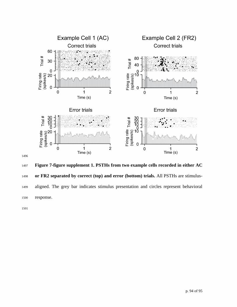
p. 94 of 95

1496

Figure 7-figure supplement 1. PSTHs from two example cells recorded in either AC 1497

or FR2 separated by correct (top) and error (bottom) trials. All PSTHs are stimulus-1498

aligned. The grey bar indicates stimulus presentation and circles represent behavioral 1499

response. 1500

1501

p. 95 of 95

# stimulus sig. # choice sig. Total #

AC CR 19 21 39

NCR 18 21 64

FR2 CR 20 22 31

NCR 10 11 43

1502

Table 1. Number of classically responsive (CR) or non-classically responsive (NCR) 1503

neurons in AC and FR2 with significant stimulus or choice information. 1504