SPI Observer's Manual - INTEGRALintegral.esac.esa.int/AO11/AO11 SPI ObsMan.pdf · 2013-02-27 ·...

INTEGRAL

Science Operations Centre

Announcement of Opportunity for Observing Proposals (AO-11)

SPI Observer's Manual INT/OAG/13-0384/Dc

Issue 1.0

4th March 2013

Prepared by C. Sánchez-Fernández

INTEGRAL SPI Observer's Manual

Doc.No: INT/OAG/13-0384/Dc

Issue: 1.0 Date: 4 March 2013 Page: 2 of 36

Based on inputs from:

J.P. Roques, SPI Co-PI, CESR Toulouse

R. Diehl, SPI Co-PI, MPE Germany




Table of Contents 1 Introduction .............................................................................................................................. 5

2 Description of the instrument ................................................................................................... 7

2.1 Overall design .................................................................................................................... 7

2.1.1 Detectors and pre-amplifiers ....................................................................................... 8

2.1.2 The detector electronics .............................................................................................. 9

2.1.3 Cryostat ....................................................................................................................... 9

2.2 Pulse Shape Discriminator (PSD)...................................................................................... 9

2.3 Anti-Coincidence Subassembly (ACS) ........................................................................... 10

2.4 The Plastic Scintillator Anti Coincidence Subassembly (PSAC) .................................... 11

2.5 Electronics ....................................................................................................................... 11

2.6 The passive mask ............................................................................................................. 11

3 Instrument operations ............................................................................................................. 13

3.1 How the instrument works ............................................................................................... 13

3.2 SPI operating modes ........................................................................................................ 13

3.3 Dead time ......................................................................................................................... 14

3.4 Telemetry budget ............................................................................................................. 14

3.5 Spectroscopy .................................................................................................................... 14

3.6 Timing ............................................................................................................................. 15

3.7 Imaging ............................................................................................................................ 15

3.8 Gamma-ray burst detection ............................................................................................. 15

4 Performance of the instrument ............................................................................................... 17

4.1 Components and sources of the SPI instrumental background ....................................... 17

4.2 Measured performance .................................................................................................... 18

4.2.1 Imaging resolution .................................................................................................... 18

4.2.2 Energy resolution ...................................................................................................... 19

4.2.3 Annealing .................................................................................................................. 21

4.2.4 Sensitivities ............................................................................................................... 22

4.2.5 Dithering sensitivity degradation .............................................................................. 23

4.2.6 Detection of off-axis sources .................................................................................... 24

4.2.7 Timing capabilities ................................................................................................... 25

4.3 Instrumental characterisation and calibration .................................................................. 25




4.4 Astronomical considerations on the use of the instrument .............................................. 27

5 Observation “Cook book” ...................................................................................................... 34

5.1 How to estimate observing times .................................................................................... 34

5.1.1 Gamma-ray line ........................................................................................................ 34

5.1.2 Gamma-ray continuum ............................................................................................. 35

5.2 Worked examples ............................................................................................................ 35




1 Introduction The SPectrometer onboard INTEGRAL (SPI) is one of the two prime instruments of the INTEGRAL scientific payload. SPI is a high spectral resolution gamma-ray telescope devoted to the observation of the sky in the 20 keV - 8 MeV energy range, using an array of 19 closely packed germanium detectors. SPI is the first high-resolution gamma-ray spectral imager to operate in this energy range. The spectral resolution is fine enough to resolve astrophysical lines and allow spectroscopy in the regime of gamma-rays. The coded mask provides imaging at moderate resolution. The main characteristics of the instrument are given in Table 1. An overall cut-away view of the instrument is shown in Figure 1.

Table 1- Main characteristics of the SPI instrument, nominal values

Detector dimensions 60 mm wide surface, 70 mm deep

Mask dimensions 665 mm flat to flat 30 mm thick Tungsten

Detector unit Encapsulated Ge, hexagonal

geometry, 19 detectors 70 mm thick

Energy range 20 keV - 8 MeV

Energy resolution (FWHM) 2.2 keV at 1.33 MeV for each

detector, 3 keV for the whole spec-trometer.

Angular resolution 2.5o for point sources

Point source positioning <1.3o for point sources (depending on point source intensity)

Field-of-view fully coded: 14o flat to flat,

16o corner to corner zero coding: 32o flat to flat,

35o corner to corner (zero sensitivity)

The science objectives of SPI are nucleosynthesis, relativistic-particle accelerators, and strong-field signatures in compact stars; this is studied through nuclear lines and spectral features in accreting binaries, pulsars, or solar flares, but also through energetic continuum radiation in the 20keV- 8MeV range from a variety of cosmic sources, including active galactic nuclei and gamma-ray bursts.

SPI is a collaborative international project developed for ESA under the responsibility of CNES Toulouse (France) as prime contractor. Subsystems for SPI have been built by: LDR and MPE (Germany; Anti-coincidence subsystem), the University of Louvain (Belgium; Germanium for detectors), CESR (France; Ge detectors and their electronics), CEA-Saclay (France; Digital Front End Electronics), CNES (France; cryostat, lower structure, flight software, thermal control), University of Valencia (Spain; coded mask), IFCTR Milano (Italy; Plastic Scintillator)




and the University of Berkeley and San Diego (USA; Pulse Shape Discriminator). The two Co-PIs responsible for the SPI instrument are J.P. Roques (CESR, Toulouse, France) and R. Diehl (MPE, Garching, Germany).

The following sections provide a description of the instrument (Section 2), its operations (Section 3), its performance (Section 4) and some hints on the use of the instrument (Section 5; “cook book”). For further details we refer the interested reader to a series of papers on the SPI instrument in the A&A special INTEGRAL issue (2003, 411, L63-L113). This issue also contains various other papers on the first results from in-flight observations. For a description of the SPI data analysis, we refer also to the special INTEGRAL issue (2003, A&A 411, L117-L127) and the SPI validation report of the Off-line-Scientific Analysis (OSA) software package released by the ISDC. Besides, the descriptions of the data analysis pipelines and modules and the use of the OSA software can be found at the ISDC website:

http://www.isdc.unige.ch/integral/analysis.




2 Description of the instrument

2.1 Overall design

Figure 1 - A cut-away view of SPI. The camera and detectors are described in sect. 2.1.1 and 2.1.2, the ACS system in sect 2.3, the PSAC in section 2.4 and the PSAC in sect. 2.6,

SPI is a coded mask spectrometer, composed of the following main subsystems:

- the camera, with 19 cooled, hexagonally shaped, high purity germanium detectors (GeDs) and their associated electronics;

- a two-stage cooling system, composed of a passive stage and an active stage;

- a pulse shape discrimination system (PSD) which allows discrimination between single and multi-site interactions in one Ge detector;




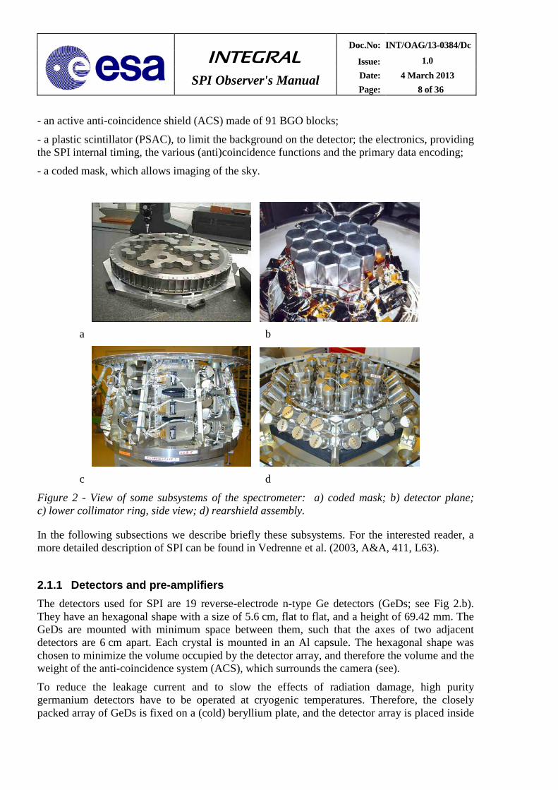
- an active anti-coincidence shield (ACS) made of 91 BGO blocks;

- a plastic scintillator (PSAC), to limit the background on the detector; the electronics, providing the SPI internal timing, the various (anti)coincidence functions and the primary data encoding;

- a coded mask, which allows imaging of the sky.

a b

c d

Figure 2 - View of some subsystems of the spectrometer: a) coded mask; b) detector plane; c) lower collimator ring, side view; d) rearshield assembly.

In the following subsections we describe briefly these subsystems. For the interested reader, a more detailed description of SPI can be found in Vedrenne et al. (2003, A&A, 411, L63).

2.1.1 Detectors and pre-amplifiers The detectors used for SPI are 19 reverse-electrode n-type Ge detectors (GeDs; see Fig 2.b). They have an hexagonal shape with a size of 5.6 cm, flat to flat, and a height of 69.42 mm. The GeDs are mounted with minimum space between them, such that the axes of two adjacent detectors are 6 cm apart. Each crystal is mounted in an Al capsule. The hexagonal shape was chosen to minimize the volume occupied by the detector array, and therefore the volume and the weight of the anti-coincidence system (ACS), which surrounds the camera (see).

To reduce the leakage current and to slow the effects of radiation damage, high purity germanium detectors have to be operated at cryogenic temperatures. Therefore, the closely packed array of GeDs is fixed on a (cold) beryllium plate, and the detector array is placed inside




a cryostat (see sect. 2.1.3). The bottom side of the cold plate houses the first stage of the preamplifier circuitry (PA-1), which has only passive components. The PA-1 electronics include the high voltage filter and the connection between the detector and the Charge Sensitive Amplifier (CSA). A second set of 19 pre-amplifiers (PA-2) is mounted on a second cold plate established at 210 K and thermally connected to the cryostat. This stage includes the FET, for which the low temperature allows a reduction of the electronic noise.

Currently, only 15 out of the 19 detectors are operated, following failures of detectors #2 in December 2003, #17 in July 2004, #5 in February 2009 and #1 in May 2010. 2.1.2 The detector electronics The signals from the pre-amplifiers are sent to the amplification chain, which is made up of a Pulse Shape Amplifier (PSA) and a Pulse Height Amplifier (PHA). The PSA amplifies the pulses such that the performance of the spectrometer is optimised. The PSA also provides a timing signal used for time-tagging each event analysed. The pulse heights are coded by the Pulse Height Analyser (PHA; 16384 channels in two energy ranges: 0-2 MeV and 2-8 MeV). For the first energy range, each channel has a resolution of 0.13 keV, while for the second range, one channel corresponds to 0.52 keV.

The detector electronics also comprise a high voltage power supply (0-5000 V) for the Ge detectors and a low voltage power supply for the pre-amplifiers (19 independent chains per amplification chain).

2.1.3 Cryostat For an optimum sensitivity and resolution, the Ge detectors must be kept at a constant cryogenic temperature. The SPI cryostat is designed to keep the detectors at the operating temperature. It also provides the functions necessary for Ge crystal annealing. The cryostat is composed of three systems: an active cooling system, a passive cooling system and a cold box.

The active cooling system brings the temperature of the cold plate, on which the detectors are mounted, down to 80 K. The cooling is obtained by 4 mechanical Stirling cycle coolers. The performance of the mechanical coolers in terms of heat lift is limited to a few Watts, so the Ge detectors have to be very well thermally insulated from their environment. Therefore, the detection plane is enclosed in a beryllium structure (cold box) controlled at an intermediate temperature (210 K) through a passive cooling device.

All temperatures of the cryostat subsystems are regularly monitored to provide the ground operators with early warnings in case of failures of the coolers, and to provide temperature information that can be used for the data processing.

2.2 Pulse Shape Discriminator (PSD)

The PSD subsystem compares the shape of the pulses produced by the pre-amplifiers, with pro-files stored in an onboard archive. It was aimed at the reduction of β-decay background in the Ge detectors. Experience obtained during the early mission revealed that using the information from the PSD does not significantly increase the signal to noise ratio: it is therefore not used currently.




2.3 Anti-Coincidence Subassembly (ACS)

The main function of the Anti-Coincidence Subassembly (ACS) is to shield the Ge detectors against background (photons and particles) from sources outside the field-of-view. The SPI ACS consists of 91 bismuth-germanate (BGO) scintillator blocks arranged in 4 subunits: two collimator rings (the upper and lower collimator ring, located between the coded mask and the detector plane) whose axes are along the viewing direction of the spectrometer; the side-shield and the rear-shield assemblies that surround the camera. The BGO crystal thickness was optimised via Monte Carlo simulations to minimize the detector background, because a too high mass of BGO can increase secondary neutron production, producing extra background in the Ge crystals.

Figure 3 – SPI background spectra of GeD events in anticoincidence with an event in the ACS ("ACS on'') and in coincidence with an event in the ACS ("vetoed only''). The total rate in the 20-8000 keV range changes by a factor of ~25 between both configurations (Jean et al. 2003, A&A vol. 411, L107).

The BGO scintillator crystals convert all incoming events into photons in the 480 nm region (visible light). Photo-multiplier tubes are then used to detect these photons and convert them into electrical pulses, which are combined into an overall veto signal. The ACS output data is directed to the Digital Front End Electronics (DFEE, see Sect. 2.5). The latter formats the data and time-tags each event. Photons that are not in coincidence with an ACS veto event are considered as “good”. Additionally, the DFEE time-tag these events, and transmit event rates at a 50 ms resolution. These can be used, e.g., for Gamma-Ray Burst (GRB) studies (see Sect 3.8 for detailed information on GRB detection by SPI/ACS). Photons that occur outside the ACS veto signal are considered, sorted, normalised and summed up by the ACS electronics.




The ACS significantly reduces the instrument background as can be seen in Figure 3, which shows the background spectra of the GeD events that did not coincide ("ACS on'') or that did coincide ("vetoed only'') with a trigger of the ACS. The total rate (in the 20 keV-8000 keV range) changes by a factor of ~25 between both configurations.

2.4 The Plastic Scintillator Anti Coincidence Subassembly (PSAC)

The purpose of the Plastic Scintillator Anti-Coincidence Subassembly (PSAC) is to reduce the 511 keV background due to particle emission by the passive mask. The PSAC consists of a plastic scintillator inside a light tight box, located just below the passive mask. It has a good gamma-ray transparency, and actively detects particles which deposit energies in excess of 300 keV. The light flashes produced by the impacts of high energy particles on the scintillator are detected with two photo-multiplier tubes located around the light-tight box and converted into electrical pulses. They are processed by the PSAC electronics assembly, which then sends to the DFEE a signal associated with the detected events, and compatible with the ACS veto signal. In-flight calibrations have shown that the PSAC provides background reductions of the order of a few %.

2.5 Electronics

The SPI electronics is divided into the Digital Front End Electronics (DFEE) and the Data Processing Electronics (DPE). The DFEE are in charge of the real-time acquisition, assembly, time-tagging and synchronization of the various signals from the SPI front end (detector electronics, PSD, ACS, etc). The DFEE subdivide the events into classes depending on their origin in the instrument and handle overall event energies and system monitoring statistics (dead time, signal counts, etc). Detected events are time-tagged with a 20 MHz local clock, which provides the timing resolution. The reset (timing reference) is done with the 8 Hz satellite clock. The statistics are passed on to the DPE every second. The DPE are part of the On-Board Data Handling (OBDH) unit. It provides the telecommand and telemetry interfaces to the instrument and the environment for the instrument dedicated software (Instrument Application Software, IASW).

2.6 The passive mask

The imaging capability of the spectrometer is obtained with the help of a coded-aperture mask, which codes the incident gamma rays in the field-of-view. The passive mask is located at the top of the instrument, above the plastic scintillator, and 171 cm from the detector plane. The distance is driven by the required field-of-view and angular resolution. The mask also provides stiffness to the primary structure of SPI.

The mask has a sandwich structure made of a nomex honeycomb core covered by two skins, a titanium ring that forms the interface to the rest of the instrument, and a coded motif made of 127 hexagonal elements. 63 of these elements are made of 3 cm thick tungsten and are opaque to gamma-ray radiation within the SPI operational range, with an absorption efficiency >95% at 1 MeV. The other 64 elements are nearly free of matter, and thus almost transparent to gamma-rays: they have a gamma-ray transparency of 60% at 20 keV and 80% at 50 keV. The imaging principle of a mask is based on the fact that each gamma-ray source in the field of view throws a shadow on the detector. Since the “shadowgrams” of different sources are independent from




each other, a deconvolution technique allows the reconstruction of sky-maps, with resolved source positions.

The mask-detector arrangement defines a fully-coded field of view of 16o × 14o (y/z dimension) and partially-coded field of view of 26o × 23o respectively. An image of the mask pattern is provided in Figure 2a.




3 Instrument operations

3.1 How the instrument works

The operating mode of SPI is based on the detection of GeD events which are in the 20 keV-8 MeV energy range, and which are not accompanied by ACS events. The events can be single detector events (SE), with photon energy deposit in only one detector, or multiple detector events (ME), which arise from an interaction cascade of a single primary photon with energy deposits in more than one detector. In this case, the sum of the energy deposits corresponds to the total energy deposited by the initial photon. All the events are processed by the DFEE, which provides event timing with 102.4 µs accuracy, event building and classification, and event rejection, using the ACS veto signal. The events are also counted and the dead time is permanently monitored. The DPE receive all the data from the DFEE, assemble all the information, and send the resulting stream to the satellite telemetry downlink system.

SPI provides a combination of high-resolution spectroscopy with imaging capabilities. The performance characteristics of the instrument depend on the instrumental design as follows:

• Energy resolution: it is determined by the cooled Ge detectors.

• Angular resolution: it is determined by the pixel size of both the mask and the detector, and by the distance between them. Since the GeD assembly consists of only 15 detectors, an image of the sky is not unambiguously defined by the “shadowgram” pattern. The ambiguity is resolved by introducing dithering steps of the telescope axis, around the direction of the gamma-ray source to be studied (dithering).

• Field-of-view: it is defined by the area of the mask, the germanium detector assembly, the distance between them, as well as the ACS shield.

• Narrow line sensitivity: achieved by making the detector as large as possible, by minimizing the background (using an ACS optimised in material and thickness), by choosing carefully the materials used in the instrument, and by adding a PSAC below the mask.

• Timing accuracy: requires a high telemetry rate, because the events are recorded photon-by-photon.

3.2 SPI operating modes

SPI has only one mode for normal observations, the so-called “photon by photon” mode, which has a high time resolution. In this mode, the scientific data are collected and transmitted to the ground for each detected (non-vetoed) photon, from which the type of event, the energy and the timing can be deduced. Furthermore, detector spectra of all events (including vetoed ones) can be accumulated and transmitted every 30-60 minutes.

In case the SPI telemetry is continuously overflowing due to background radiation higher than expected, or due to a strong solar flare, the instrument can be operated in a “degraded” science mode (TM emergency mode). In this case, the on-board processing and transmission of data will be restricted to “good” events (non-vetoed). The maximum data generation rate in this mode




will be about half the rate for normal photon by photon mode. The observer cannot select the TM emergency mode: in case it is needed, ground controllers command it.

Before any change of mode, the SPI instrument will be put into a special configuration mode. This is the only mode in which changes to the instrument configuration can be made. SPI will not be taking scientific data when in configuration mode (science telemetry processing is stopped). Several other special modes are available for engineering tasks (e.g., annealing) and for instrument calibrations; they are not of interest to the general observer.

3.3 Dead time

Due to several causes (e.g., veto signals), within a normal exposure, a dead time occurs during which no useful scientific data are collected. The amount of dead time depends on several external conditions (e.g., increase of the ACS rate during a solar flare). Experience obtained during previous AOs has shown that the SPI dead time is about 15% of the observing time.

3.4 Telemetry budget

INTEGRAL uses packet telemetry (TM). Each packet corresponds to 0.44 kbps. For SPI, the background mainly determines the telemetry usage. The telemetry allocated to SPI was changed several times since the launch of INTEGRAL to be adapted to the real background, and to follow its evolution (for example, it depends on the solar activity). Since October 2010, the TM allocation for SPI is 99 packets per cycle.

3.5 Spectroscopy

In the standard observing mode, the instrument can be used for spectroscopic observations. In the energy range of SPI, the signal-to-background ratio is in general small (typically a few to 10%). Knowing the background is critical to produce high quality gamma-ray spectra. Furthermore, the background in each of the 19 (15 currently operational) independent detectors can vary in time in a different way, further limiting the instrument sensitivity.

To solve the uncertainties in the background determination, an appropriate dithering strategy has to be adopted for every observation (see the “Overview, Policies and Procedures” document for further details). Dithering is also important to improve the image quality of the reconstructed sky images (see sect. 3.7). Therefore, all SPI observations should use dithering, since background calculation for staring observations is very difficult, if not impossible, due to background in-homogeneities over the detector plane.

The dithering strategy to be adopted should be preferably 5x5, because it is well suited for observations of a region containing multiple or complex sources, or for sources whose position is poorly known. It is also well suited for observations of extended or weak sources that can best be studied by accumulating exposure time through a sum of individual pointings. This observation mode should always be used as the default.

The use of the hex mode is discouraged, because it seriously compromises the imaging capabilities of SPI, rendering the data useless for use in large mosaics with or without using archival data, and, as such it renders the data useless for any investigation of high energy emission from celestial sources using SPI. Therefore, the use of the hexagonal mode must be very well motivated (see sect 3.7).




3.6 Timing

In the standard observing mode (photon by photon), SPI can be used for timing analysis. The data set for each photon includes timing information given by a 102.4 µs clock signal. This clock is synchronised to the on-board clock, and thus to the UTC, allowing for the instrument timing capabilities.

3.7 Imaging

In the photon by photon mode, the (x,y) coordinates of each event detected are registered and a “shadowgram” (i.e., a detector-plane image of the coded-mask shadow) is constructed. The sky image results from the deconvolution of the shadowgram, and the pattern of the mask. The imaging performance of SPI depends on the dithering pattern used: in general, the larger the number of pointings executed, the better the image reconstruction.

Users must be aware that when using the hexagonal dither pattern, the reconstructed point source response function shows very strong side lobes at distances of 10o to 20o from the centre. Therefore, the observers are discouraged to use this mode. The side lobes are still present, but significantly less with the 5 by 5 dither pattern (about 50% of the hexagonal case). To remove these side lobes, which will cause artefacts in the reconstructed sky images, the only possibility is to enlarge the imaged area by observing multiple pointings (i.e., multiple dither patterns).

3.8 Gamma-ray burst detection

One important contribution of the ACS to the science obtained with SPI is its use as a GRB monitor. The ACS shield provides a large effective area for the detection of bursts; unfortunately, the electronics impedes spatial resolution of the detection, because only the total event rate of all crystals with 50 ms time resolution is sent down to Earth through TM packets. Therefore, accurate positions of gamma ray bursts that are detected with the ACS have to be determined through triangulation methods, with other (distant) spacecrafts. The INTEGRAL Science Data Centre (ISDC) software checks the stream of veto count rates automatically. If a gamma ray burst is detected (sudden increase in the count rate over a short period of time), an alert is issued to the 3rd Interplanetary Network (IPN) of gamma-ray bursts detectors. From the accurate timing of the SPI detection and detections by other spacecraft, a position is constructed and communicated to the scientific community. The accuracy that can be achieved with this method is much better than an arcminute (due to the long baseline, and the accurate timing of the SPI ACS events). The SPI-ACS data do not include spectral information because the energy of the interacting gamma-ray photons is not measured. The ACS events are written to the instrument Housekeeping and are therefore made public immediately. Observers can be notified of these GRB events by subscribing to the INTEGRAL gamma-ray Burst Alert System (IBAS) of the ISDC: http://www.isdc.unige.ch/integral/ibas/ibasclnt_regform.html. Information on the SPI/ACS triggers since the start of the mission is available from this URL.

The SPI ACS detects a rate of 0.3 true GRB per day. It has now detected more than 800 confirmed cosmic GRBs. These are events which have been observed by at least one other experiment in the interplanetary network (IPN). The weakest event, confirmed so far, is GRB071112, with a fluence of 4.8 × 10-8 erg cm-2.

http://www.isdc.unige.ch/integral/ibas/ibasclnt_regform.html




The SPI-ACS has also detected over 476 events confirmed as soft gamma repeaters (SGRs). For example, about 45 short bursts and one giant flare were detected from the magnetar SGR1806-20 (Mereghetti et al. 2005), and several short bursts from SGR1900+14. Strong flaring activity from the anomalous X-ray pulsar 1E 1547.0-5408 was detected by the ACS on Jan 2009, when more than 200 bursts were detected within a few hours (Mereghetti et al. 2009, ApJ, 696, 74)

A review of the highlights of the SPI-ACS detections can be found in Hurley et al. 2010 (Proceedings of the 8th INTEGRAL Workshop. 27 - 30 September 2010 Dublin, Ireland. Available from http://pos.sissa.it/cgi-bin/reader/conf.cgi?confid=115; see also Rau et al. 2005, A&A, 438, 1175).

http://pos.sissa.it/cgi-bin/reader/conf.cgi?confid=115




4 Performance of the instrument

4.1 Components and sources of the SPI instrumental background

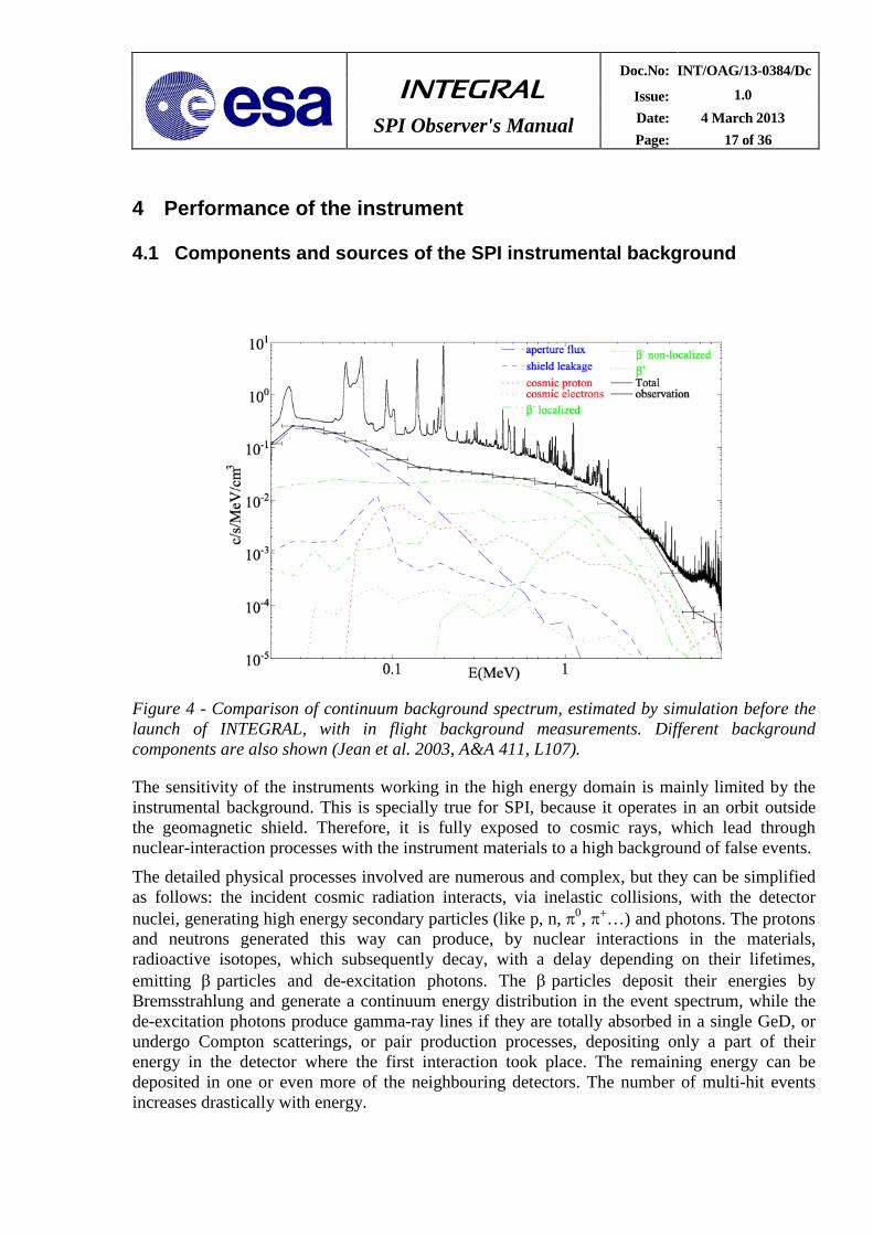
Figure 4 - Comparison of continuum background spectrum, estimated by simulation before the launch of INTEGRAL, with in flight background measurements. Different background components are also shown (Jean et al. 2003, A&A 411, L107).

The sensitivity of the instruments working in the high energy domain is mainly limited by the instrumental background. This is specially true for SPI, because it operates in an orbit outside the geomagnetic shield. Therefore, it is fully exposed to cosmic rays, which lead through nuclear-interaction processes with the instrument materials to a high background of false events.

The detailed physical processes involved are numerous and complex, but they can be simplified as follows: the incident cosmic radiation interacts, via inelastic collisions, with the detector nuclei, generating high energy secondary particles (like p, n, π0, π+…) and photons. The protons and neutrons generated this way can produce, by nuclear interactions in the materials, radioactive isotopes, which subsequently decay, with a delay depending on their lifetimes, emitting β particles and de-excitation photons. The β particles deposit their energies by Bremsstrahlung and generate a continuum energy distribution in the event spectrum, while the de-excitation photons produce gamma-ray lines if they are totally absorbed in a single GeD, or undergo Compton scatterings, or pair production processes, depositing only a part of their energy in the detector where the first interaction took place. The remaining energy can be deposited in one or even more of the neighbouring detectors. The number of multi-hit events increases drastically with energy.




In addition to these genuine gamma-ray events, there are other background events created in the detector via elastic neutron scatterings, which can only partially be recognized as background events.

The SPI background spectrum measured in flight is shown in Figure 4, which also plots the contribution of the various processes to the continuum. For further information on the SPI instrumental background and its variations, we refer the reader to Jean et al. 2003, A&A, 411, L107; for information on the identification and modelling of the SPI background lines see Weidenspointner et al. 2003, A&A, 411, L113 and references therein.

4.2 Measured performance 4.2.1 Imaging resolution The SPI imaging performance is highly dependent upon the analysis method, the complexity of the field observed (in terms of number of sources, their flux stability, and their relative intensity) and the background handling. Note, however, that although the background is not uniformly distributed on the camera, its shape, determined from empty field observations for each energy bin, is relatively stable (Roques et al. 2003 A&A 411, L91). The imaging capabilities of SPI are illustrated in Figure 5 (see also Bouchet et al. 2008, ApJ 679, 1315, for results on deeper exposures).

Figure 5 - The Galactic plane as observed by SPI during the Galactic Center Deep Exposure (GCDE) observation. Energy range: 20-50 keV (Roques et al. 2003, A&A, 411, L113)




The measured angular resolution for (isolated) point sources is about 2.5o (FWHM). This is the width of the instrument response correlation for a point source. Point sources can be located with better accuracy, but this depends on the strength of the source (the significance over the background) and locations of nearby sources. Strong sources can be located to an accuracy of 0.5 arcminute, while sources closer than 2 degrees will not be discriminated though imaging (see Dubath et al. 2005, MNRAS, 357, 420).

Positions measured by SPI have an uncertainty that is mainly statistical, and therefore count rate dependent. The uncertainties decrease as the inverse of the detection significance, and range from ~10 to ~1 arcminute for detection significances of ~10 to ~100. For higher detection significances (e.g., the Crab), the detection is ultimately limited to ~0.5 arcminute in position.

4.2.2 Energy resolution

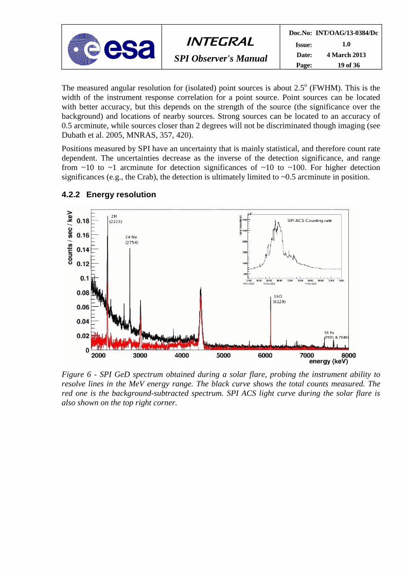
Figure 6 - SPI GeD spectrum obtained during a solar flare, probing the instrument ability to resolve lines in the MeV energy range. The black curve shows the total counts measured. The red one is the background-subtracted spectrum. SPI ACS light curve during the solar flare is also shown on the top right corner.




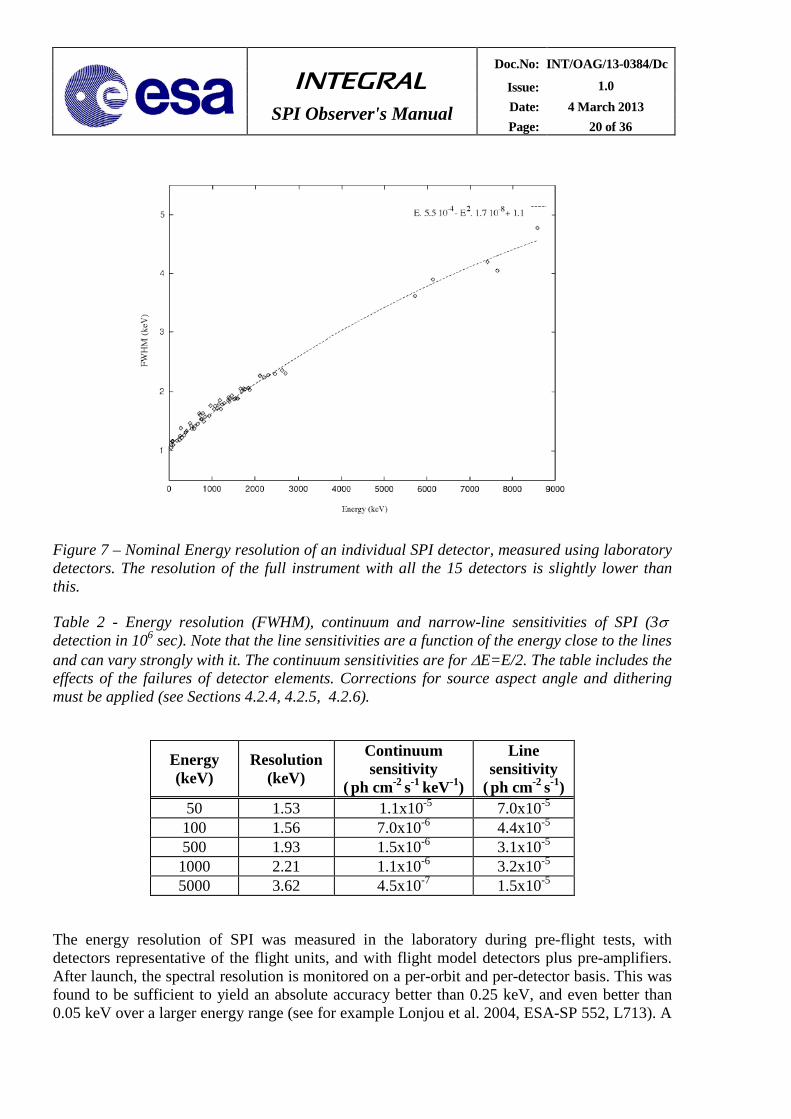
Figure 7 – Nominal Energy resolution of an individual SPI detector, measured using laboratory detectors. The resolution of the full instrument with all the 15 detectors is slightly lower than this.

Table 2 - Energy resolution (FWHM), continuum and narrow-line sensitivities of SPI (3σ detection in 106 sec). Note that the line sensitivities are a function of the energy close to the lines and can vary strongly with it. The continuum sensitivities are for ∆E=E/2. The table includes the effects of the failures of detector elements. Corrections for source aspect angle and dithering must be applied (see Sections 4.2.4, 4.2.5, 4.2.6).

Energy (keV)

Resolution (keV)

Continuum sensitivity

( ph cm-2 s-1 keV-1)

Line sensitivity

( ph cm-2 s-1) 50 1.53 1.1x10-5 7.0x10-5 100 1.56 7.0x10-6 4.4x10-5 500 1.93 1.5x10-6 3.1x10-5 1000 2.21 1.1x10-6 3.2x10-5 5000 3.62 4.5x10-7 1.5x10-5

The energy resolution of SPI was measured in the laboratory during pre-flight tests, with detectors representative of the flight units, and with flight model detectors plus pre-amplifiers. After launch, the spectral resolution is monitored on a per-orbit and per-detector basis. This was found to be sufficient to yield an absolute accuracy better than 0.25 keV, and even better than 0.05 keV over a larger energy range (see for example Lonjou et al. 2004, ESA-SP 552, L713). A




spectrum measured in-flight, during a solar flare, is shown in Figure 6 to illustrate the capability of SPI to revolve lines in the MeV domain. The energy resolution measured for an individual detector is shown in Figure 7, and the energy resolution for the full instrument is given in Table 2. The observers should be aware that in regimes of strong instrumental lines (such as the 511 keV line), the sensitivities are significantly worse than in between such lines.

The energy resolution of the GeDs evolves with time, and a continuous monitoring of the resolution is needed to analyse properly the data from SPI. This is because the GeD performance degrades with the damages created within the crystal by incident radiation (mainly protons and neutrons). This increases the number of hole traps within the active detection volume. In space, the particle flux is high enough to produce substantial degradation of the GeDs over times of a few months (about 20% in 6 months). The damage is not permanent and can be corrected by the annealing procedure.

4.2.3 Annealing

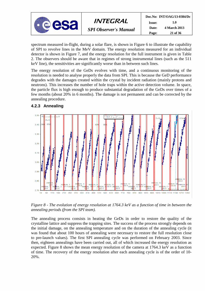
Figure 8 - The evolution of energy resolution at 1764.3 keV as a function of time in between the annealing periods (from the SPI team).

The annealing process consists in heating the GeDs in order to restore the quality of the crystalline lattice and suppress the trapping sites. The success of the process strongly depends on the initial damage, on the annealing temperature and on the duration of the annealing cycle (it was found that about 100 hours of annealing were necessary to restore the full resolution close to pre-launch values). The first SPI annealing cycle was performed on February 2003. Since then, eighteen annealings have been carried out, all of which increased the energy resolution as expected. Figure 8 shows the mean energy resolution of the camera at 1764.3 keV as a function of time. The recovery of the energy resolution after each annealing cycle is of the order of 10-20%.




4.2.4 Sensitivities The instrument performance numbers (energy resolution, continuum and line sensitivities) at specific energies are shown in Table 2. The sensitivities provided in this table correspond to 3σ detections in 106 seconds of pure integration time. The quoted sensitivities only include the statistical errors, the impact of imaging algorithm and background subtraction methods are not included. The line sensitivities indicated are for narrow lines. The continuum sensitivities are for ∆E=E, and are calculated from the narrow line sensitivity by dividing those by ER ∆⋅ , where R is the instrument resolution for lines. The sensitivity limit is 4.8x10-5 ph cm-2 s-1 at 511 keV, and 3.1x10-5 ph cm-2s-1 at 1809 keV. The continuum and line sensitivities of SPI are displayed in Figure 9 and Figure 10, respectively. The users should also be aware that the 511 sensitivity is worse than the surrounding continuum, due to the strong 511 keV background line originating in the instrument.

Figure 9 - The continuum sensitivity of SPI for an on-axis, 3σ detection in 106 seconds. Fluxes are for ∆E=E/2. Corrections for failures of detector #1, #2, #5 and #17 have been considered. Corrections for source aspect angle and dithering must be applied when necessary (see Sect. 4.2.5, 4.2.6).

Note that the failures of detectors #1, 2, 5 and 17 imply the loss of single events from these detector units, and an increase of the single-event rates in neighbouring detectors from the former multiple-events of #1, 2, 5 and 17 (scattering into neighbouring detectors). The sensitivity loss thus depends on the event type selection, and corresponds to between 5% for continuum and 20% for low-energy lines. The sensitivity Figures (9, 10) are for the 15-element Ge camera, hence they include these effects, as well as the loss in sensitivity caused by the current high background associated to the solar minimum.




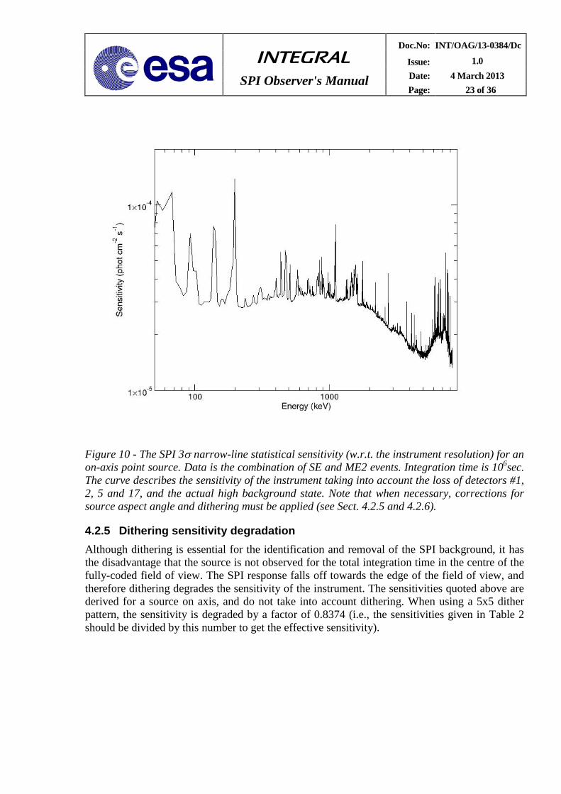
Figure 10 - The SPI 3σ narrow-line statistical sensitivity (w.r.t. the instrument resolution) for an on-axis point source. Data is the combination of SE and ME2 events. Integration time is 106sec. The curve describes the sensitivity of the instrument taking into account the loss of detectors #1, 2, 5 and 17, and the actual high background state. Note that when necessary, corrections for source aspect angle and dithering must be applied (see Sect. 4.2.5 and 4.2.6).

4.2.5 Dithering sensitivity degradation Although dithering is essential for the identification and removal of the SPI background, it has the disadvantage that the source is not observed for the total integration time in the centre of the fully-coded field of view. The SPI response falls off towards the edge of the field of view, and therefore dithering degrades the sensitivity of the instrument. The sensitivities quoted above are derived for a source on axis, and do not take into account dithering. When using a 5x5 dither pattern, the sensitivity is degraded by a factor of 0.8374 (i.e., the sensitivities given in Table 2 should be divided by this number to get the effective sensitivity).




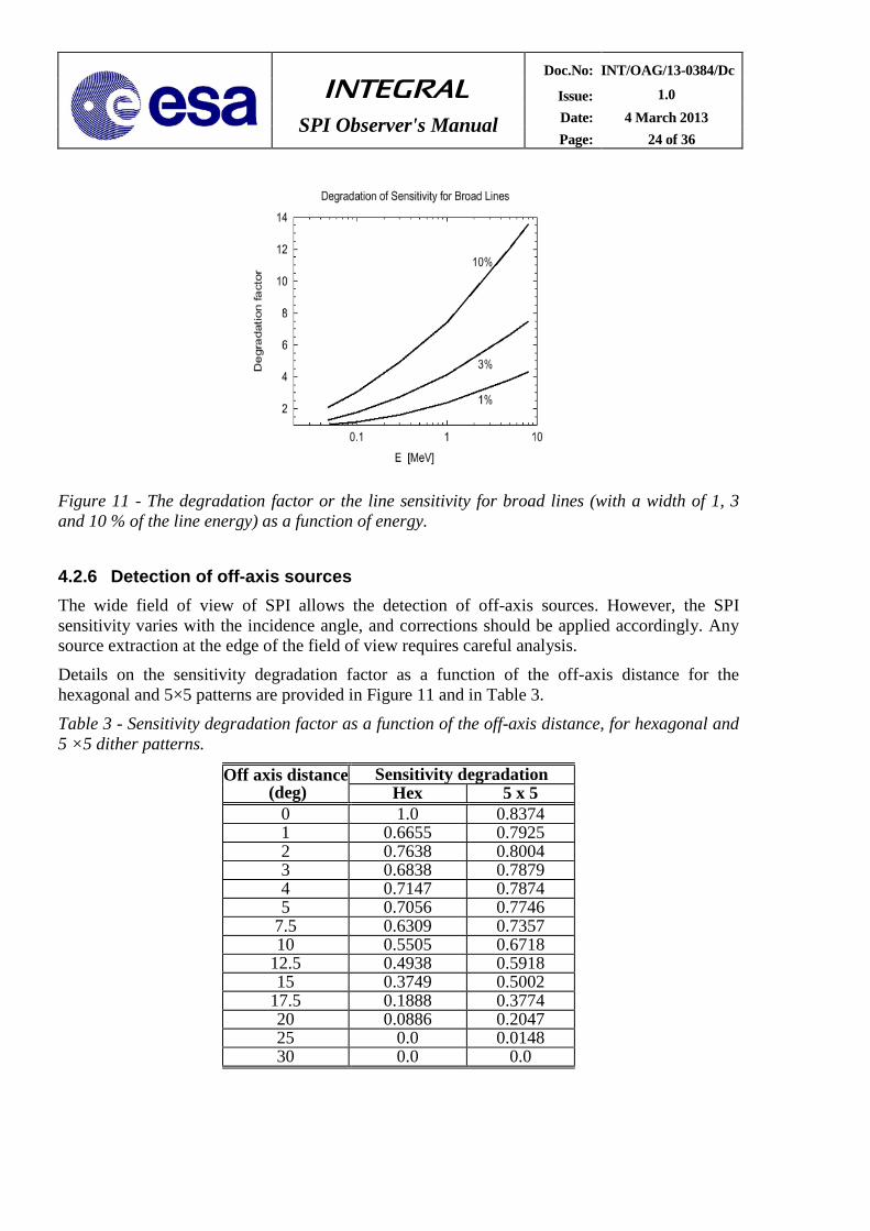
Figure 11 - The degradation factor or the line sensitivity for broad lines (with a width of 1, 3 and 10 % of the line energy) as a function of energy.

4.2.6 Detection of off-axis sources The wide field of view of SPI allows the detection of off-axis sources. However, the SPI sensitivity varies with the incidence angle, and corrections should be applied accordingly. Any source extraction at the edge of the field of view requires careful analysis.

Details on the sensitivity degradation factor as a function of the off-axis distance for the hexagonal and 5×5 patterns are provided in Figure 11 and in Table 3.

Table 3 - Sensitivity degradation factor as a function of the off-axis distance, for hexagonal and 5 ×5 dither patterns.

Off axis distance (deg)

Sensitivity degradation Hex 5 x 5

0 1.0 0.8374 1 0.6655 0.7925 2 0.7638 0.8004 3 0.6838 0.7879 4 0.7147 0.7874 5 0.7056 0.7746

7.5 0.6309 0.7357 10 0.5505 0.6718

12.5 0.4938 0.5918 15 0.3749 0.5002

17.5 0.1888 0.3774 20 0.0886 0.2047 25 0.0 0.0148 30 0.0 0.0




4.2.7 Timing capabilities In the standard photon by photon mode, each photon data set includes timing information given by a 102.4 µs clock signal. This clock is synchronised to the on-board clock, and thus to the U.T.C. There are, however small uncertainties affecting the event time accuracy, namely:

• the accuracy of the on-board clock and the synchronisation;

• the conversion between on-board time and U.T.C.;

• the conversion between U.T.C. arrival time at the spacecraft and the arrival time at the solar system barycentre.

The resulting timing resolution of SPI is 129 µs (3σ accuracy) with a 90% confidence accuracy of 94 µs. Timing analysis of the Crab data has revealed that the absolute timing accuracy is about 40 µs (1σ uncertainty; see Kuiper et al. 2003, A&A 411, L31).

The capabilities of SPI to perform timing analysis are illustrated in Figure 12, which shows the pulse profile of the Crab pulsar, as measured by the spectrograph.

Note that due to strict limits on the telemetry allocation, SPI was operated during a large part of AO1 in a mode where the single event photons were only downloaded as part of the histograms, severely degrading the time resolution for these events to 30 minutes. The increased telemetry budget for SPI allowed to restore the original time resolution for single events. Therefore, in combining new observations with data from the 2002-early 2003 period, a proper operation mode data must be selected.

4.3 Instrumental characterisation and calibration

The SPI instrument was tested and calibrated with radioactive sources on ground, before the launch. Further testing was performed during the Performance and Verification (PV) phase of the mission, and has been carried out thereafter by conducting regular calibration observations. The sensitivities, resolution, and other characteristics given in this document represent the current best knowledge of the SPI instrumental characterisation.

Figure 12 - Phase histogram of the Crab pulsar (PSR B0531+21; P=33 ms) as measured by SPI (20-100 keV, phase resolution of 0.0025). Phase 1 is that of the main radio pulse. The inner panels magnify the main pulse and the interpulse peaks. (Molkov et al. 2010, ApJ, 708, 410).




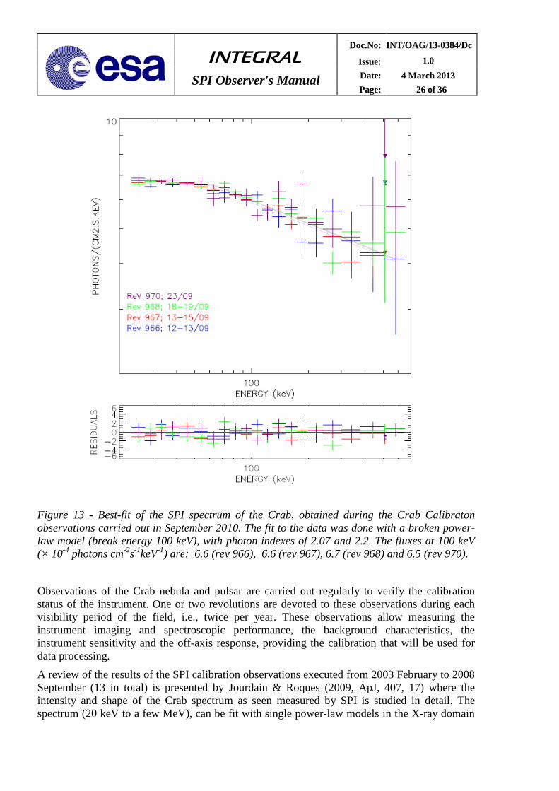
Figure 13 - Best-fit of the SPI spectrum of the Crab, obtained during the Crab Calibraton observations carried out in September 2010. The fit to the data was done with a broken power-law model (break energy 100 keV), with photon indexes of 2.07 and 2.2. The fluxes at 100 keV (× 10-4 photons cm-2s-1keV-1) are: 6.6 (rev 966), 6.6 (rev 967), 6.7 (rev 968) and 6.5 (rev 970).

Observations of the Crab nebula and pulsar are carried out regularly to verify the calibration status of the instrument. One or two revolutions are devoted to these observations during each visibility period of the field, i.e., twice per year. These observations allow measuring the instrument imaging and spectroscopic performance, the background characteristics, the instrument sensitivity and the off-axis response, providing the calibration that will be used for data processing.

A review of the results of the SPI calibration observations executed from 2003 February to 2008 September (13 in total) is presented by Jourdain & Roques (2009, ApJ, 407, 17) where the intensity and shape of the Crab spectrum as seen measured by SPI is studied in detail. The spectrum (20 keV to a few MeV), can be fit with single power-law models in the X-ray domain




(mean photon index ~2.05) and MeV domain (photon index ~2.23) with an energy break close to 100 keV. Further details can be found in the aforementioned paper.

The spectrum of the Crab as measured by SPI during the latest calibration observations executed in September 2010 is shown in Figure 13. The fit to the data is consistent with a broken power-law model (break energy 100 keV), with photon indexes of 2.07 and 2.2.

Crab calibration observations are also used to study and improve the cross calibration between the INTEGRAL instruments. There are now very little systematic differences in the residuals from one Crab observation to the other and a very good match between IBIS/ISGRI and SPI. For further details in the status of the IBIS/SPI cross calibration we refer the reader to the ISDC Astrophysics Newsletter, #21, and the “Overview, Policies and Procedures” document.

Instrumental background lines are also used to calibrate the instrument. Being originated in the instrument itself, instrumental lines are not expected to be intrinsically broadened or shifted due to the Doppler effect. Lines originating in the BGO shield (e.g. 511 keV, 6.1 MeV O line) are currently used for energy calibration, whereas the lines that originate from materials inside the cryostat (and have known intensities) can be used to measure the Ge detector efficiency. These calibrations are carried out once per revolution and per detector.

The detector gains, thresholds and resolution versus energy are determined from normal event data and ACS off spectra (for consistency checks) in the routine monitoring task of ISDC. Finally, after every detector annealing, a thorough check of the instrument imaging and spectroscopic response is done, since these may change as a result of the annealing process.

4.4 Astronomical considerations on the use of the instrument

SPI is designed as a spectrometer; therefore it should primarily be used for high-resolution spectroscopy on sources with (narrow) lines, possibly on top of a continuum. Given the imaging qualities of the instrument, it can also be used for wide field imaging of diffuse emission, especially in (narrow) emission lines. However, if high resolution imaging observations of sources with only continuum emission, or very broad lines are needed, the IBIS instrument might be better suited as a prime instrument, at least below a few hundred keV.

Table 4 - Some gamma-ray lines from cosmic radioactivity in the SPI energy range.

Isotope decay chain line energies (MeV)

Mean life (year)

e+ E++e-photon 0.511 ~1x105 56Co (56Ni) 56Co 56Fe 0.847, 1.238 0.31 22Na 22Na 22Ne 1.275 3.8 44Ti 44Ti 44Sc 44Ca 1.156 89 26Al 26Al 26Mg 1.809 1.0x106 60Fe 60Fe 60Co 60Ni 1.173,1.322 2.2x106




The prime astrophysical topics to be addressed with SPI are: nucleosynthesis processes, super-nova theories, nova theories, interstellar physics and pair plasma physics in compact objects (neutron stars, black holes). A number of interesting astrophysical lines fall in the SPI energy range, some of them are compiled in Table 4.

We now present a summary of some results obtained with SPI to illustrate its capabilities (the selection is by no means exhaustive).

Thanks to its large field of view and to the dithering strategy, SPI is optimum for imaging large sky areas, through the combination of a large set of individual pointings. For example, this has allowed the generation of maps of diffuse continuum and line emission in the Galaxy (see Figure 14). The continuum images of the Galaxy reveal the transition from a point source dominated hard X-ray sky to a diffuse emission dominated soft gamma-ray sky (Figure 14; Bouchet et al. 2008, ApJ 679, 1315, and references therein).

Figure 14 – SPI sky maps in the 25-50 keV (top, left), 50-100 keV (top, right), 100-200 keV (bottom, left) and 200-600 keV (bottom, right) energy bands. The images are scaled logarithmically with a rainbow color map.The scale is saturated to reveal the weakest sources. At low energy, the sky emission is dominated by sources, while a "diffuse/extended" structure appears above 200-300 keV, in a domain corresponding to the annihilation radiation. These images have been obtained by maximum-likelihood fitting of point sources from a reference catalogue, plus diffuse-emission models represented from a set of pixons (16×2.6 deg in size). From Bouchet et al. 2008, Ap,J 679, 1315.




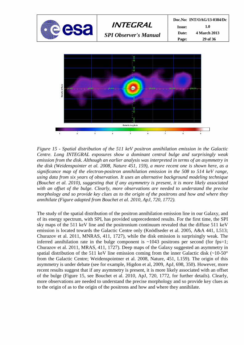
Figure 15 - Spatial distribution of the 511 keV positron annihilation emission in the Galactic Centre. Long INTEGRAL exposures show a dominant central bulge and surprisingly weak emission from the disk. Although an earlier analysis was interpreted in terms of an asymmetry in the disk (Weidenspointer et al. 2008, Nature 451, 159), a more recent one is shown here, as a significance map of the electron-positron annihilation emission in the 508 to 514 keV range, using data from six years of observation. It uses an alternative background modeling technique (Bouchet et al. 2010), suggesting that if any asymmetry is present, it is more likely associated with an offset of the bulge. Clearly, more observations are needed to understand the precise morphology and so provide key clues as to the origin of the positrons and how and where they annihilate (Figure adapted from Bouchet et al. 2010, ApJ, 720, 1772). The study of the spatial distribution of the positron annihilation emission line in our Galaxy, and of its energy spectrum, with SPI, has provided unprecedented results. For the first time, the SPI sky maps of the 511 keV line and the positronium continuum revealed that the diffuse 511 keV emission is located towards the Galactic Centre only (Knödlseder et al. 2005, A&A 441, L513; Churazov et al. 2011, MNRAS, 411, 1727), while the disk emission is surprisingly weak. The inferred annihilation rate in the bulge component is ~1043 positrons per second (for fps=1; Churazov et al. 2011, MRAS, 411, 1727). Deep maps of the Galaxy suggested an asymmetry in spatial distribution of the 511 keV line emission coming from the inner Galactic disk (~10-50° from the Galactic Centre; Weidenspointner et al. 2008, Nature, 451, L159). The origin of this asymmetry is under debate (see for example, Higdon et al, 2009, ApJ, 698, 350). However, more recent results suggest that if any asymmetry is present, it is more likely associated with an offset of the bulge (Figure 15, see Bouchet et al. 2010, ApJ, 720, 1772, for further details). Clearly, more observations are needed to understand the precise morphology and so provide key clues as to the origin of as to the origin of the positrons and how and where they annihilate.




The superb energy resolution of SPI has allowed, moreover, detailed spectral modelling of the annihilation emission in the 400-600 keV range. Three components of the line emission have been observed: a narrow (2 keV) line at 511 keV, a broad (5 keV) component, and a continuum emission due to the decay of ortho-positronium at energies below 511 keV (Figure 16; see Jean et al. 2006, A&A 445, L579, for further details).

Away from the Galactic center, the disc emission contains a prominent 1809 keV gamma-ray line from 26Al. SPI images in the 1809 keV gamma-ray have confirmed the basic emission features established by COMPTEL: a strong Galactic ridge emission from the inner Galaxy, and prominent features from different regions which host young stars in the Galaxy such as the Cygnus region (Knödlseder et al. 2007, ESA Conf. Proc. SP-622, 13), Sco-Cen or Cas A. Moreover, the spatially-resolved spectroscopy allowed by SPI has shown that the 26Al line centroid traces the bulk motion imposed by large-scale rotation within the Galaxy. A minor redshift (0.1 keV) is measured for positive longitudes, but a significant blueshift (0.4 − 0.8 keV) is detected for negative longitudes with respect to the 1809 keV emission observed from the Galactic Centre (Wang et al. 2009, A&A, 496, 713; Diehl et al. 2006, Nature, 439, L45). For a detailed view of the 26Al distribution along the plane of the Galaxy see Figure 17. 60Fe decay gamma-ray lines 1173 keV and 1333 keV have also been measured by SPI. Almost three years of data provided a 4.9 σ detection of 60Fe from the Galactic plane. The average 60Fe line flux from the inner Galaxy region is 4.4 ± 0.9 x10-5 ph cm-2 s-1 rad-1 . From this dataset, the ratio of 60Fe to 26Al was derived to be ~ 15%, a value consistent with current theoretical models (Wang et al. 2007, A&A, 469, L1005). 60Fe emission from the Cygnus and Vela regions has not been detected yet.

Figure 16 - Spectrum of the electron-positron 511 keV annihilation emission, showing the narrow and broad line components and the continuum emission below 511 keV due to the decay of ortho-positronium. (Jean et al. 2006, A&A, 445, L579).




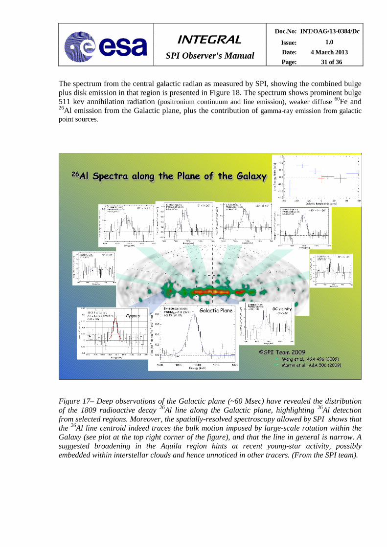
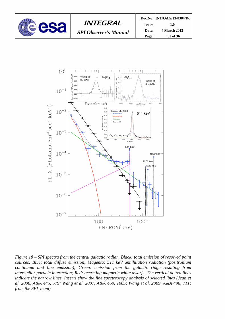
The spectrum from the central galactic radian as measured by SPI, showing the combined bulge plus disk emission in that region is presented in Figure 18. The spectrum shows prominent bulge 511 kev annihilation radiation (positronium continuum and line emission), weaker diffuse 60Fe and 26Al emission from the Galactic plane, plus the contribution of gamma-ray emission from galactic point sources.

Figure 17– Deep observations of the Galactic plane (~60 Msec) have revealed the distribution of the 1809 radioactive decay 26Al line along the Galactic plane, highlighting 26Al detection from selected regions. Moreover, the spatially-resolved spectroscopy allowed by SPI shows that the 26Al line centroid indeed traces the bulk motion imposed by large-scale rotation within the Galaxy (see plot at the top right corner of the figure), and that the line in general is narrow. A suggested broadening in the Aquila region hints at recent young-star activity, possibly embedded within interstellar clouds and hence unnoticed in other tracers. (From the SPI team).




Figure 18 – SPI spectra from the central galactic radian. Black: total emission of resolved point sources; Blue: total diffuse emission; Magenta: 511 keV annihilation radiation (positronium continuum and line emission); Green: emission from the galactic ridge resulting from interstellar particle interaction; Red: accreting magnetic white dwarfs. The vertical dotted lines indicate the narrow lines. Inserts show the fine spectroscopy analysis of selected lines (Jean et al. 2006, A&A 445, 579; Wang et al. 2007, A&A 469, 1005; Wang et al. 2009, A&A 496, 711; from the SPI team).




To complement its suitability in the study of diffuse emission, the spectrometer SPI has also proved its superb capabilities in the study of point-like emission in the hard X-ray and soft gamma-ray regime. The SPI all-sky survey analysis, based on 4 years of SPI observations (~51 Msec), has also provided a complete catalogue of 173, 79, 30, and 12 sources detected above ~3.5-σ in the 25-50 and 50-100 keV bands and above ~2.5-σ in the 100-200 and 200-600 keV bands (Bouchet et al. 2008, ApJ, 679, 1315). All but one are associated (within 1°) with at least one IBIS source (Bird et al. 2007, ApJS, 170, 175). Above 600 keV, only the Crab Nebula, Cyg X-1, GRS 1915+105, and GRS 1758-258 are detected, the former two objects still emitting above 2 MeV.




5 Observation “Cook book”

5.1 How to estimate observing times

The formal way to calculate accurate observing time is via the Observing Time Estimator (OTE), which can be found at: http://integral.esac.esa.int/isocweb/ote.htmlis/////However, in this section we provide an easy way for observers to estimate the observing times using simple formulae. The times calculated in this way are reasonably accurate, and are for most cases within a few percent from the OTE calculated times. In the worked examples we show both estimations for comparisons. Note, however, that ISOC will only use the OTE to assess the technical feasibility of the proposals. General observers can request observations of a gamma-ray line (flux expressed as ph cm-2 s-1), or observations of the integrated continuum flux over a certain energy band (flux also expressed in ph cm-2 s-1). Examples of both instances are presented in the following examples.

Note: the observers should make sure that observing times entered into PGT allow the completion of at least one full dither pattern (i.e., minimum of 12600 seconds for an hexagonal dither and 45000 seconds for a 5 x 5 dither). 5.1.1 Gamma-ray line The observation time, Tobs (in kiloseconds), is estimated using the relation:

deadracline

lineobs fR

EFF

SNT

−⋅

∆⋅

⋅

⋅⋅⋅=1

13

1012

3 σ ,

where:

- Nσ is the sigma required in the detection;

- Sline is the 3σ, on-axis point source, SPI narrow line sensitivity at the considered energy, for 106 s integration time and 100% live-time. The values of this parameter are shown in Table 2;

- Fline is the source line flux in ph cm-2 s-1;

- Frac is the sensitivity degradation factor due to dithering, or to the source being off-axis. See Table 3, Sections 4.2.5 and 4.2.6 for details;

− ∆E is the expected width of the gamma-ray line (FWHM in keV);

- R is the energy resolution of the spectrometer (in keV). It depends on the energy. The values of this parameter are given in Table 2; - fdead is the fraction of dead-time (15%). This parameter is described in Section 3.3.

http://integral.esac.esa.int/isocweb/ote.ht




5.1.2 Gamma-ray continuum The observation time, Tobs (in kiloseconds), is estimated using the relation:

deadracline

lineobs fR

EFF

SNT

−⋅

∆⋅

⋅

⋅⋅⋅=1

15.13

1012

3 σ

deadraccont

cont

fEE

FFSN

−⋅

∆⋅

⋅

⋅⋅⋅=1

123

1012

3 σ ,

where:

− Fint is the flux integrated over the specified band (in ph cm-2 s-1);

− Fcont is the continuum flux in the specified band (in ph cm-2 s-1 keV-1);

− ∆E is the width of the energy band corresponding to the specified flux (in keV);

− Scont is the continuum sensitivity as given in Table 2. The continuum sensitivity can be calculated from the line sensitivity, using:

ERSS linecont ∆= 5.1/

All other parameters are as described above. The factor 1.5 is used to correct the gamma-ray line sensitivity, which is calculated assuming that the total counts in a line are contained in an energy band of 1.5 times the spectral resolution (FWHM). Actually, 1.5 times the resolution contains ~95% of the line counts.

In previous versions of the OTE, the band over which the flux is specified should not be too broad (maximum ∆E=E/2) since the sensitivities were for ∆E=E/2. However, with the latest versions of the OTE, observers can specify a power-law slope and then the OTE will split the total energy band up into many small bands, and combine all the results.

5.2 Worked examples

In this section we present some examples of observations with SPI for which we calculated the observing times with the formulae given above, and the OTE. Note that for lines, the exposure time derived from the OTE differs from the one calculated from the formula. This is because the OTE uses sensitivities at a much higher energy resolution than tabulated in Table 2 (see Figure 7). The examples below (for lines) are therefore only intended as an order of magnitude estimate; one should use the exposure times obtained with the OTE.

Example 1a: the 26Al line at 1809 keV, with a width of 3 keV (FWHM), and an integrated flux of 5x10-5 ph cm-2 s-1, to be observed with a 5x5 dither pattern. The requested significance is 3σ. The sensitivity at this energy is 3.09x10-5 ph cm-2 s-1, the resolution is 2.553 keV, and the sensitivity degradation factor for the 5x5 dither pattern is 0.8374. Using these numbers, the required observing time would be 756 ksec (the OTE gives 603 ksec).




Example 1b, to show the correspondence between the manual and the OTE results at an energy where the line sensitivity is fairly constant: a line at 2000 keV, with a 3 keV width, and a inte-grated line flux of 5x10-5 ph cm-2 s-1, observed with a 5x5 dither pattern. The requested significance is 3σ. The sensitivity at this energy is 2.75x10-5 ph cm-2 s-1, the resolution is 2.634 keV, and the sensitivity degradation factor for the 5x5 dither is, again, 0.8374. With these numbers, the required observing time would be 588 ksec (the OTE gives 557 ksec).

Example 2: the same 1809 keV line, but now observed with an hexagonal dither (sensitivity degradation factor of 1.0) for a significance of 3σ would require 405 ksec, (however, keep in mind that this is true only for isolated point sources; the OTE gives 423 ksec).

Example 3: a continuum band of 150 keV width, centred at 350 keV, with a continuum flux of 2x10-5 ph cm-2 s-1 keV-1; observed with a 5x5 dither for a significance of 10σ. The continuum sensitivity for this energy is 1.8x10-6 ph cm-2 s-1 keV-1, the resolution is 1.80 keV, and the sensitivity degradation factor is again 0.8374. This observation would then require 134 ksec, (the OTE gives 185 ksec with an in-band flux of 3.0x10-3 ph cm-2 s-1).

Example 4: the 44Ti line at 1.160 MeV in a supernova remnant (e.g., Cas A). The line width is 2000 km s-1 (or 7.73 keV), the integrated line flux 1x10-4 ph cm-2 s-1. The source should be observed with a 5x5 dither, for a significance of 5σ. The sensitivity of the instrument at this energy is 3.06x10-5 ph cm-2 s-1, the resolution is 2.28 keV, and the sensitivity degradation factor is again 0.8374. The required observing time would then be 1.48 Msec (the OTE gives 1.46 Msec).

Example 5: a broad, red-shifted 511 keV line. The energy of the line is 465 keV, with a width of 5000 km s-1 (or 16 keV), and an integrated line flux of 3.3x10-4 ph cm-2 s-1. The observation is to be performed using the hexagonal dithering mode (isolated source), for a significance of 5σ. The sensitivity of the instrument at this energy is 3.53x10-5 ph cm-2 s-1, the energy resolution is 1.93 keV and the sensitivity degradation factor is 1.0. This observation would then need 310 ksec (the OTE gives 408 ksec).

Example 6: a continuum band of 500 keV width, centred at 4 MeV, with a continuum flux of 1x10-6 ph cm-2 s-1 keV-1. The observation should use a 5x5 dither pattern, and requires a 3σ detection. The sensitivity of the instrument at this energy is 4.1x10-7 ph cm-2 s-1 keV-1, the resolution is 3.32 keV and the sensitivity degradation factor is 0.8374. This observation would require 916 ksec (the OTE gives 1.2 Msec, assuming a constant photon flux over the energy band, giving a flux of 5x10-4 ph cm-2s-1 in this band).

Example 7: an extended source with a size of 4.8 degrees and a continuum flux of 2x10-5 photons cm-2 s-1 keV-1 in a band of 150 keV, centred at 350 keV. With an angular resolution of 2.5 degrees, the source can be resolved in (4.8/2.5)2 pixels. In 134 ks, a sensitivity of 10/(4.8/2.5) (see example 3), or 5.2σ, can be reached.

SPI Observer's Manual - INTEGRALintegral.esac.esa.int/AO11/AO11 SPI ObsMan.pdf · 2013-02-27 ·...

Documents

Transcript of SPI Observer's Manual - INTEGRALintegral.esac.esa.int/AO11/AO11 SPI ObsMan.pdf · 2013-02-27 ·...