spgrambw: Plot Spectrograms in MATLAB

Mike Brookes

Version: 1639, 15/03/2012

Contents

1 Introduction 1

2 Function call 2

3 Colour maps 2

4 Frequency axis 34.1 Nonlinear frequency scaling . . . . . . . . . . . . . . . . . . . . . . . . . . . . . . . . . . . . . . . 34.2 Frequency range and stepsize . . . . . . . . . . . . . . . . . . . . . . . . . . . . . . . . . . . . . . 3

5 Analysis bandwidth 4

6 Time Axis 4

7 Intensity scaling 5

8 Waveform and transcription 5

9 Output Arguments 6

10 MODE string options 6

11 MATLAB Code for figures 7

1 Introduction

This document describes the spgrambw function which is part of the voicebox toolbox available at http://

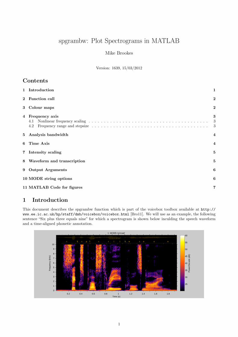
www.ee.ic.ac.uk/hp/staff/dmb/voicebox/voicebox.html [Bro11]. We will use as an example, the followingsentence “Six plus three equals nine” for which a spectrogram is shown below inculding the speech waveformand a time-aligned phonetic annotation.

Time (s)

Fre

quen

cy (

kHz)

1: MODE='pJcwat'

s � k s p l � s � r i i k w � z n a� n

0.2 0.4 0.6 0.8 1 1.2 1.4 1.6 1.8

0

1

2

3

4

5

6

7

8

9

10

Pow

er/D

ecad

e (d

B)

25

30

35

40

45

50

55

60

1

2 Function call

The basic call to the function is:

[T, F ,B]=spgrambw (S , FS ,MODE,BW,FMAX,DB,TINC,ANN)

where all but the first two input arguments are optional. The input arguments are:

S input speech waveform

FS sample rate of speech waveform

MODE text string specifying a large range of options

BW the bandwidth of the spectrogram. This argument determines the tradeoff between time and frequencyresolution.

FMAX specifies the range and resolution of the frequency axis

DB specifies the range of power spectral density displayed

TINC specifies the range and resolution of the time axis

ANN gives an optional annotation file containing words or phonemes.

If all you want to do is draw a spectrogram, then the function should be called without any output arguments.If output arguments are specified, then no spectrogram will be drawn unless the ’g’ mode option is also given.The output arguments are

T gives the time of each time-axis sample point

F gives the frequency of each frequency-axis sample point

B a 2-dimensional array giving the spectral density at each time-frequency point.

In the plots shown in this document, the title (above the spectrogram) shows the figure number (written {n}in the text), the value of the MODE argument and the value of any other arguments that are not null.

3 Colour maps

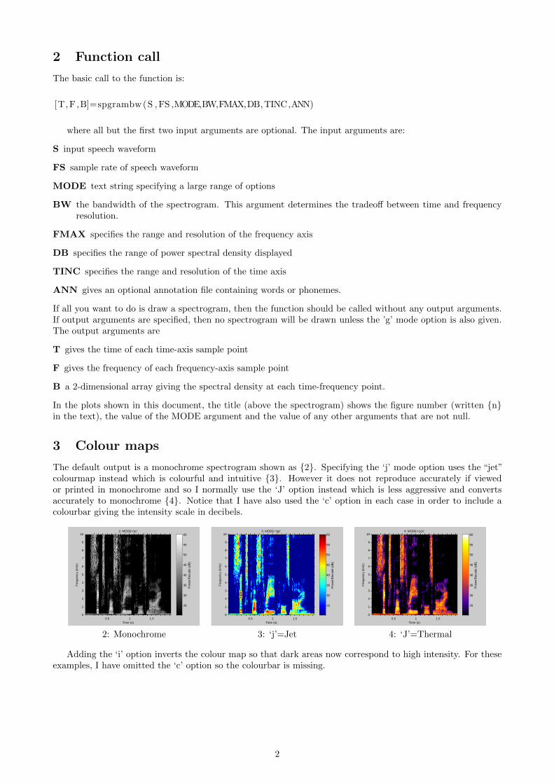
The default output is a monochrome spectrogram shown as {2}. Specifying the ‘j’ mode option uses the “jet”colourmap instead which is colourful and intuitive {3}. However it does not reproduce accurately if viewedor printed in monochrome and so I normally use the ‘J’ option instead which is less aggressive and convertsaccurately to monochrome {4}. Notice that I have also used the ‘c’ option in each case in order to include acolourbar giving the intensity scale in decibels.

Time (s)

Fre

quen

cy (

kHz)

2: MODE='pc'

0.5 1 1.50

1

2

3

4

5

6

7

8

9

10

Pow

er/D

ecad

e (d

B)

25

30

35

40

45

50

55

60

Time (s)

Fre

quen

cy (

kHz)

3: MODE='pjc'

0.5 1 1.50

1

2

3

4

5

6

7

8

9

10

Pow

er/D

ecad

e (d

B)

25

30

35

40

45

50

55

60

Time (s)

Fre

quen

cy (

kHz)

4: MODE='pJc'

0.5 1 1.50

1

2

3

4

5

6

7

8

9

10

Pow

er/D

ecad

e (d

B)

25

30

35

40

45

50

55

60

2: Monochrome 3: ‘j’=Jet 4: ‘J’=Thermal

Adding the ‘i’ option inverts the colour map so that dark areas now correspond to high intensity. For theseexamples, I have omitted the ‘c’ option so the colourbar is missing.

2

Time (s)

Fre

quen

cy (

kHz)

5: MODE='pi'

0.5 1 1.50

1

2

3

4

5

6

7

8

9

10

Time (s)

Fre

quen

cy (

kHz)

6: MODE='pji'

0.5 1 1.50

1

2

3

4

5

6

7

8

9

10

Time (s)

Fre

quen

cy (

kHz)

7: MODE='pJi'

0.5 1 1.50

1

2

3

4

5

6

7

8

9

10

5: ‘i’= Inverted Monochrome 6: ‘ij’=Inverted Jet 7: ‘iJ’=Inverted Thermal

4 Frequency axis

4.1 Nonlinear frequency scaling

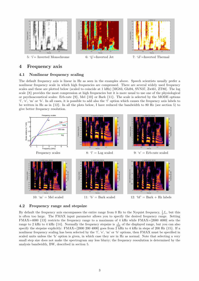
The default frequency axis is linear in Hz as seen in the examples above. Speech scientists usually prefer anonlinear frequency scale in which high frequencies are compressed. There are several widely used frequencyscales and these are plotted below (scaled to coincide at 1 kHz) [MG83, Ghi94, SVN37, Zwi61, ZT80]. The logscale {8} provides the most compression at high frequencies but it is more usual to use one of the physiologicalor psychoacoustical scales: Erb-rate {9}, Mel {10} or Bark {11}. The scale is selected by the MODE options‘l’, ‘e’, ‘m’ or ‘b’. In all cases, it is possible to add also the ‘f’ option which causes the frequency axis labels tobe written in Hz as in {12}. In all the plots below, I have reduced the bandwidth to 80 Hz (see section 5) togive better frequency resolution.

0 1 2 3 4 5 60

0.5

1

1.5

2

2.5

3

Frequency (kHz)

Frequency scales

lin

log

mel

bark

erb-rate

Time (s)

Fre

quen

cy (

log 10

Hz)

8: MODE='pJcl', BW=80

0.5 1 1.5

1.6

1.8

2

2.2

2.4

2.6

2.8

3

3.2

3.4

3.6

3.8

4

Pow

er/D

ecad

e (d

B)

25

30

35

40

45

50

55

60

Time (s)

Fre

quen

cy (

Erb

-rat

e)

9: MODE='pJce', BW=80

0.5 1 1.50

2

4

6

8

10

12

14

16

18

20

22

24

26

28

30

32

Pow

er/D

ecad

e (d

B)

25

30

35

40

45

50

55

60

Frequency scales 8: ‘l’ = Log scaled 9: ‘e’ = Erb-rate scaled

Time (s)

Fre

quen

cy (

kMel

)

10: MODE='pJcm', BW=80

0.5 1 1.50

0.2

0.4

0.6

0.8

1

1.2

1.4

1.6

1.8

2

2.2

2.4

2.6

2.8

3

Pow

er/D

ecad

e (d

B)

25

30

35

40

45

50

55

60

Time (s)

Fre

quen

cy (

Bar

k)

11: MODE='pJcb', BW=80

0.5 1 1.50

2

4

6

8

10

12

14

16

18

20

22

Pow

er/D

ecad

e (d

B)

25

30

35

40

45

50

55

60

Time (s)

Bar

k-sc

aled

fre

quen

cy (

Hz)

12: MODE='pJcbf', BW=80

0.5 1 1.50

500

1k

2k

5k

10k

Pow

er/D

ecad

e (d

B)

25

30

35

40

45

50

55

60

10: ‘m’ = Mel scaled 11: ‘b’ = Bark scaled 12: ‘bf’ = Bark + Hz labels

4.2 Frequency range and stepsize

By default the frequency axis encompasses the entire range from 0 Hz to the Nyquist frequency, 12fs, but this

is often too large. The FMAX input parameter allows you to specify the desired frequency range. SettingFMAX=4000 {13} restricts the frequency range to a maximum of 4 kHz while FMAX=[2000 4000] sets therange to 2 kHz to 4 kHz {14}. Normally the frequency stepsize is 1

256 of the displayed range, but you can alsospecify the stepsize explicitly: FMAX=[2000 200 4000] goes from 2 kHz to 4 kHz in steps of 200 Hz {15}. If anonlinear frequency scaling has been selected by the ‘l’, ‘e’, ‘m’ or ‘b’ options, then FMAX must be specified inscaled units unless the ‘h’ option is given, in which case they are in Hz as normal. Note that selecting a verysmall step size does not make the spectrogram any less blurry; the frequency resoulution is determined by theanalysis bandwidth, BW, described in section 5.

3

Time (s)

Fre

quen

cy (

kHz)

13: MODE='hpJc', FMAX=4000

0.5 1 1.50

0.5

1

1.5

2

2.5

3

3.5

4

Pow

er/D

ecad

e (d

B)

25

30

35

40

45

50

55

60

Time (s)

Fre

quen

cy (

kHz)

14: MODE='hpJc', FMAX=[2000 4000]

0.5 1 1.52

2.2

2.4

2.6

2.8

3

3.2

3.4

3.6

3.8

4

Pow

er/D

ecad

e (d

B)

25

30

35

40

45

50

55

60

Time (s)

Fre

quen

cy (

kHz)

15: MODE='hpJc', FMAX=[2000 200 4000]

0.5 1 1.5

2

2.2

2.4

2.6

2.8

3

3.2

3.4

3.6

3.8

4

Pow

er/D

ecad

e (d

B)

20

25

30

35

40

45

50

55

13: 0 to 4 kHz 14: 2 to 4 kHz 15: 200 Hz resolution

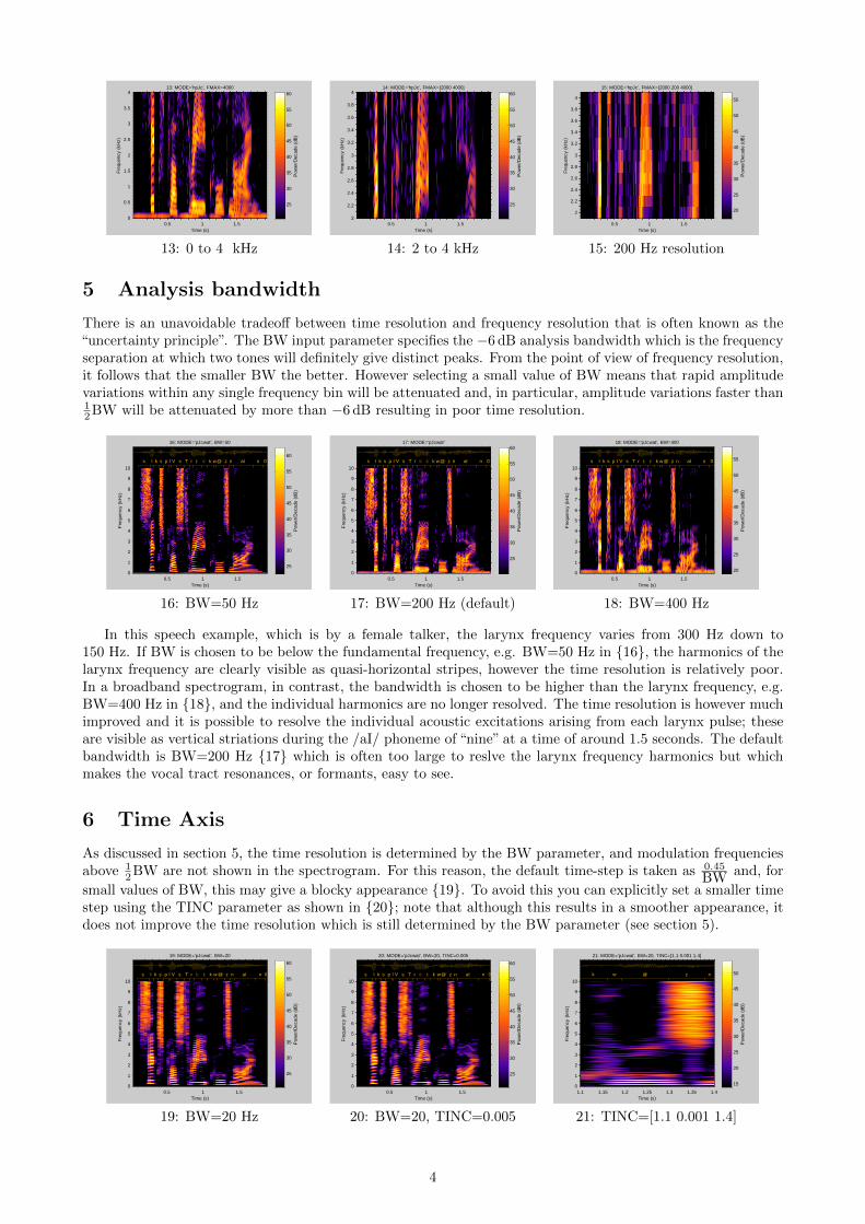
5 Analysis bandwidth

There is an unavoidable tradeoff between time resolution and frequency resolution that is often known as the“uncertainty principle”. The BW input parameter specifies the −6 dB analysis bandwidth which is the frequencyseparation at which two tones will definitely give distinct peaks. From the point of view of frequency resolution,it follows that the smaller BW the better. However selecting a small value of BW means that rapid amplitudevariations within any single frequency bin will be attenuated and, in particular, amplitude variations faster than12BW will be attenuated by more than −6 dB resulting in poor time resolution.

Time (s)

Fre

quen

cy (

kHz)

16: MODE='pJcwat', BW=50

s I k s p l V s T r i: i: k w@ z n aI n 0

0.5 1 1.50

1

2

3

4

5

6

7

8

9

10

Pow

er/D

ecad

e (d

B)

25

30

35

40

45

50

55

60

Time (s)

Fre

quen

cy (

kHz)

17: MODE='pJcwat'

s I k s p l V s T r i: i: k w@ z n aI n 0

0.5 1 1.50

1

2

3

4

5

6

7

8

9

10

Pow

er/D

ecad

e (d

B)

25

30

35

40

45

50

55

60

Time (s)

Fre

quen

cy (

kHz)

18: MODE='pJcwat', BW=400

s I k s p l V s T r i: i: k w@ z n aI n 0

0.5 1 1.50

1

2

3

4

5

6

7

8

9

10

Pow

er/D

ecad

e (d

B)

20

25

30

35

40

45

50

55

16: BW=50 Hz 17: BW=200 Hz (default) 18: BW=400 Hz

In this speech example, which is by a female talker, the larynx frequency varies from 300 Hz down to150 Hz. If BW is chosen to be below the fundamental frequency, e.g. BW=50 Hz in {16}, the harmonics of thelarynx frequency are clearly visible as quasi-horizontal stripes, however the time resolution is relatively poor.In a broadband spectrogram, in contrast, the bandwidth is chosen to be higher than the larynx frequency, e.g.BW=400 Hz in {18}, and the individual harmonics are no longer resolved. The time resolution is however muchimproved and it is possible to resolve the individual acoustic excitations arising from each larynx pulse; theseare visible as vertical striations during the /aI/ phoneme of “nine” at a time of around 1.5 seconds. The defaultbandwidth is BW=200 Hz {17} which is often too large to reslve the larynx frequency harmonics but whichmakes the vocal tract resonances, or formants, easy to see.

6 Time Axis

As discussed in section 5, the time resolution is determined by the BW parameter, and modulation frequenciesabove 1

2BW are not shown in the spectrogram. For this reason, the default time-step is taken as 0.45

BW and, for

small values of BW, this may give a blocky appearance {19}. To avoid this you can explicitly set a smaller timestep using the TINC parameter as shown in {20}; note that although this results in a smoother appearance, itdoes not improve the time resolution which is still determined by the BW parameter (see section 5).

Time (s)

Fre

quen

cy (

kHz)

19: MODE='pJcwat', BW=20

s I k s p l V s T r i: i: k w @ z n aI n 0

0.5 1 1.50

1

2

3

4

5

6

7

8

9

10

Pow

er/D

ecad

e (d

B)

25

30

35

40

45

50

55

60

Time (s)

Fre

quen

cy (

kHz)

20: MODE='pJcwat', BW=20, TINC=0.005

s I k s p l V s T r i: i: k w@ z n aI n 0

0.5 1 1.50

1

2

3

4

5

6

7

8

9

10

Pow

er/D

ecad

e (d

B)

25

30

35

40

45

50

55

60

Time (s)

Fre

quen

cy (

kHz)

21: MODE='pJcwat', BW=20, TINC=[1.1 0.001 1.4]

k w @ z n

1.1 1.15 1.2 1.25 1.3 1.35 1.40

1

2

3

4

5

6

7

8

9

10

Pow

er/D

ecad

e (d

B)

15

20

25

30

35

40

45

50

19: BW=20 Hz 20: BW=20, TINC=0.005 21: TINC=[1.1 0.001 1.4]

4

You can restrict the display to a specific time interval by setting TINC = [tmin tmax] or TINC = [tmin tstep tmax]if you want to specifiy the time-step as well {21}. Notice in {21} that the waveform and annotations remaincorrectly aligned.

The sample time of S(1) is assumed by default to be T1 = 1FS , but you can set it to any other value by

making the second input argument a vector: [FS T1].

7 Intensity scaling

The default spectrogram shows the spectral density in units of “power per Hz” {22}. Because most speechenergy is concentrated at low frequencies, this can make it difficult to see detail in the display at both low andhigh frequencies. To avoid this, you can use the ‘p’ option to display “power per decade” instead: this optionmultiplies the power by a value proportional to the frequency and so emphasises high frequencies {23}. If youare using one of the non-linear frequency scaling options described in section 4.1, you have a third option whichis to show “power per bark/erb/...” {24}.

Time (s)

Fre

quen

cy (

kHz)

22: MODE='Jc'

0.5 1 1.50

1

2

3

4

5

6

7

8

9

10

Pow

er/H

z (d

B)

-10

-5

0

5

10

15

20

25

Time (s)

Fre

quen

cy (

kHz)

23: MODE='pJc'

0.5 1 1.50

1

2

3

4

5

6

7

8

9

10

Pow

er/D

ecad

e (d

B)

25

30

35

40

45

50

55

60

Time (s)

Bar

k-sc

aled

fre

quen

cy (

Hz)

24: MODE='PJcbf'

0.5 1 1.50

500

1k

2k

5k

10k

Pow

er/B

ark

(dB

)

10

15

20

25

30

35

40

45

122: Power/Hz 23: ‘p’=Power/Decade 24: ‘P’=Power per Bark

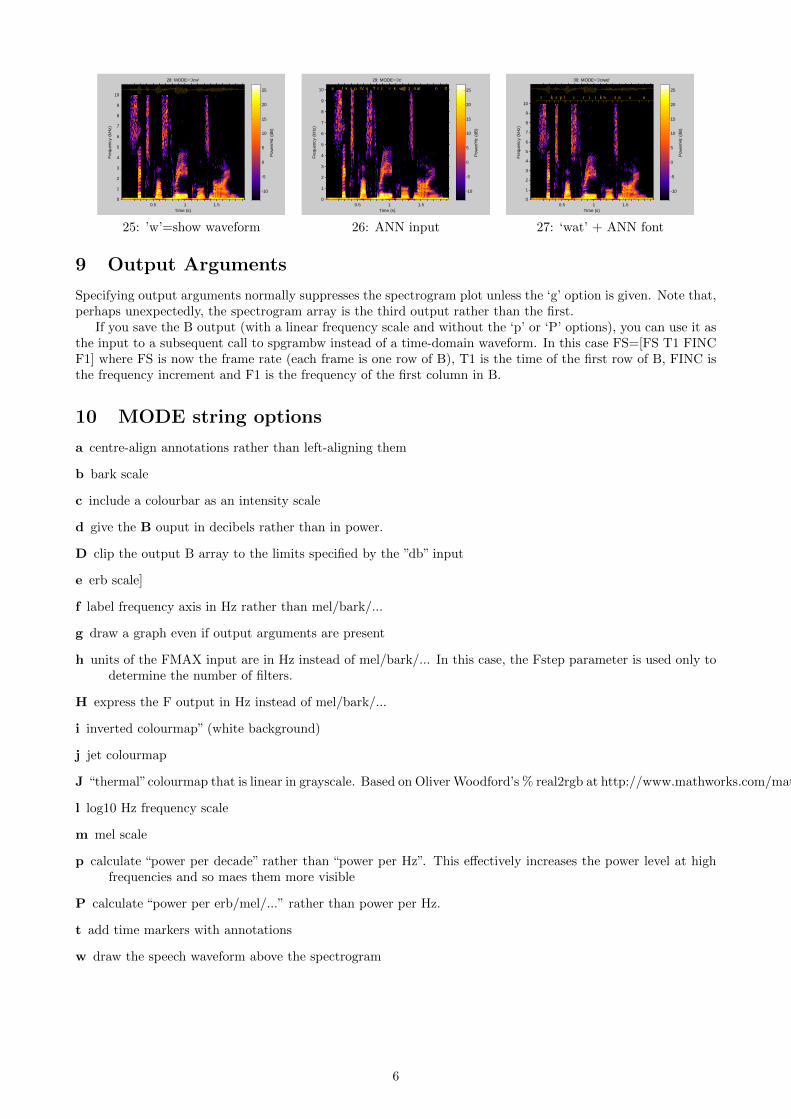
Normally, the display shows a range of 40 dB from the maximum power anywhere in the spectrrogram{25}. You can change this to a different range by setting the DB parameter either to the desired range{26}or alternatively to the minimum and maximum powers to display: DB = [Pmin Pmax] {27}. This option isespecially useful if you want to have several spectriograms with identical displayed power ranges. Values outsidethe selected range will be set to either the minimum or maximum.

Time (s)

Fre

quen

cy (

kHz)

25: MODE='Jc'

0.5 1 1.50

1

2

3

4

5

6

7

8

9

10

Pow

er/H

z (d

B)

-10

-5

0

5

10

15

20

25

Time (s)

Fre

quen

cy (

kHz)

26: MODE='Jc', DB=60

0.5 1 1.50

1

2

3

4

5

6

7

8

9

10

Pow

er/H

z (d

B)

-30

-20

-10

0

10

20

Time (s)

Fre

quen

cy (

kHz)

27: MODE='Jc', DB=[-25 0]

0.5 1 1.50

1

2

3

4

5

6

7

8

9

10

Pow

er/H

z (d

B)

-25

-20

-15

-10

-5

0

25: 40 dB range (default) 26: DB=60 27: DB=[-25 0]

8 Waveform and transcription

It is often helpful to display the time-domain waveform on the spectrogram and you can do so with th ‘w’ option{25}. If you have a transcription or other time-aligned annotation, you can specify it as the ANN input. Eachrow of the ANN cell array is of the form {[tstart tend] ‘text’}. By default, the annotations are left-aligned withintheir time intervals without any time markers {26}. If you want to display phonetic characters, you will needto install a non-unicode IPA font such as the SIL93 fonts (available for download from the Voicebox website).You can specify the font of each annotation entry by including a third column; each row of ANN is now of theform {[tstart tend] ‘text’ ‘font’}. Example {27} uses the ‘SILDoulos IPA93’ font and also includes the options ‘a’which centres the annotations in their time interval and ‘t’ which includes time markers.

5

Time (s)

Fre

quen

cy (

kHz)

28: MODE='Jcw'

0.5 1 1.50

1

2

3

4

5

6

7

8

9

10

Pow

er/H

z (d

B)

-10

-5

0

5

10

15

20

25

Time (s)

Fre

quen

cy (

kHz)

29: MODE='Jc'

s I k s p lV s T r i: i: k w@ z n aI n 0

0.5 1 1.50

1

2

3

4

5

6

7

8

9

10

Pow

er/H

z (d

B)

-10

-5

0

5

10

15

20

25

Time (s)

Fre

quen

cy (

kHz)

30: MODE='Jcwat'

s � k s p l � s � r i i k w � z n a� n

0.5 1 1.50

1

2

3

4

5

6

7

8

9

10

Pow

er/H

z (d

B)

-10

-5

0

5

10

15

20

25

25: ’w’=show waveform 26: ANN input 27: ‘wat’ + ANN font

9 Output Arguments

Specifying output arguments normally suppresses the spectrogram plot unless the ‘g’ option is given. Note that,perhaps unexpectedly, the spectrogram array is the third output rather than the first.

If you save the B output (with a linear frequency scale and without the ‘p’ or ‘P’ options), you can use it asthe input to a subsequent call to spgrambw instead of a time-domain waveform. In this case FS=[FS T1 FINCF1] where FS is now the frame rate (each frame is one row of B), T1 is the time of the first row of B, FINC isthe frequency increment and F1 is the frequency of the first column in B.

10 MODE string options

a centre-align annotations rather than left-aligning them

b bark scale

c include a colourbar as an intensity scale

d give the B ouput in decibels rather than in power.

D clip the output B array to the limits specified by the ”db” input

e erb scale]

f label frequency axis in Hz rather than mel/bark/...

g draw a graph even if output arguments are present

h units of the FMAX input are in Hz instead of mel/bark/... In this case, the Fstep parameter is used only todetermine the number of filters.

H express the F output in Hz instead of mel/bark/...

i inverted colourmap” (white background)

j jet colourmap

J “thermal”colourmap that is linear in grayscale. Based on Oliver Woodford’s % real2rgb at http://www.mathworks.com/matlabcentral/fileexchange/23342

l log10 Hz frequency scale

m mel scale

p calculate “power per decade” rather than “power per Hz”. This effectively increases the power level at highfrequencies and so maes them more visible

P calculate “power per erb/mel/...” rather than power per Hz.

t add time markers with annotations

w draw the speech waveform above the spectrogram

6

11 MATLAB Code for figures

The following code was used to generate all the figures in this document:

% demonstrat ions f o r the spgrambw t u t o r i a lc l e a r a l l ;c l o s e a l l ;p={1 2 .5 ’ pJcwat ’ [ ] [ ] [ ] [ ] 2 ;

2 1 .33 ’ pc ’ [ ] [ ] [ ] [ ] 0 ;3 1 .33 ’ pjc ’ [ ] [ ] [ ] [ ] 0 ;4 1 .33 ’ pJc ’ [ ] [ ] [ ] [ ] 0 ;5 1 .33 ’ pi ’ [ ] [ ] [ ] [ ] 0 ;6 1 .33 ’ p j i ’ [ ] [ ] [ ] [ ] 0 ;7 1 .33 ’ pJi ’ [ ] [ ] [ ] [ ] 0 ;8 1 .33 ’ pJcl ’ 80 [ ] [ ] [ ] 0 ;9 1 .33 ’ pJce ’ 80 [ ] [ ] [ ] 0 ;10 1 .33 ’pJcm ’ 80 [ ] [ ] [ ] 0 ;11 1 .33 ’ pJcb ’ 80 [ ] [ ] [ ] 0 ;12 1 .33 ’ pJcbf ’ 80 [ ] [ ] [ ] 0 ;13 1 .33 ’ hpJc ’ [ ] [ 4 0 0 0 ] [ ] [ ] 0 ;14 1 .33 ’ hpJc ’ [ ] [ 2000 4000 ] [ ] [ ] 0 ;15 1 .33 ’ hpJc ’ [ ] [ 2000 200 4000 ] [ ] [ ] 0 ;16 1 .33 ’ pJcwat ’ [ 5 0 ] [ ] [ ] [ ] 1 ;17 1 .33 ’ pJcwat ’ [ ] [ ] [ ] [ ] 1 ;18 1 .33 ’ pJcwat ’ [ 4 0 0 ] [ ] [ ] [ ] 1 ;19 1 .33 ’ pJcwat ’ [ 2 0 ] [ ] [ ] [ ] 1 ;20 1 .33 ’ pJcwat ’ [ 2 0 ] [ ] [ ] [ 0 . 0 0 5 ] 1 ;21 1 .33 ’ pJcwat ’ [ 2 0 ] [ ] [ ] [ 1 . 1 0 .001 1 . 4 ] 1 ;22 1 .33 ’ Jc ’ [ ] [ ] [ ] [ ] 0 ;23 1 .33 ’ pJc ’ [ ] [ ] [ ] [ ] 0 ;24 1 .33 ’ PJcbf ’ [ ] [ ] [ ] [ ] 0 ;25 1 .33 ’ Jc ’ [ ] [ ] [ ] [ ] 0 ;26 1 .33 ’ Jc ’ [ ] [ ] [ 6 0 ] [ ] 0 ;27 1 .33 ’ Jc ’ [ ] [ ] [−25 0 ] [ ] 0 ;28 1 .33 ’Jcw ’ [ ] [ ] [ ] [ ] 0 ;29 1 .33 ’ Jc ’ [ ] [ ] [ ] [ ] 1 ;30 1 .33 ’ Jcwat ’ [ ] [ ] [ ] [ ] 2} ;

y f i g =420; % he ight o f f i g u r e semf=1; % s e t to 1 to p r in targs ={ ’BW’ ’FMAX’ ’DB’ ’TINC’ } ;

% read the SFS−format speech f i l e

fn =’ a t05 f0 . s f s ’ ;[ sp , f s ]= r e a d s f s ( fn , 1 , 1 ) ; % speech s i g n a l[ pt , fw]= r e a d s f s ( fn , 5 , 2 ) ; % phonet ic t r a n s c r i p t i o nann=[ mat2ce l l ( [ c e l l 2mat ( pt ( : , 1 ) ) ce l l 2mat ( pt ( : , 1 : 2 ) ) ∗ [ 1 ; 1 ] ] / fw , ones (1 , s i z e ( pt , 1 ) ) ) pt ( : , 3 ) ] ;ipa=ann ( : , [ 1 2 2 ] ) ;

ipa ( : , 2 )={ ’ s ’ ’ I ’ ’ k ’ ’ s ’ ’p ’ ’ l ’ ’A’ ’ s ’ ’T’ ’ r ’ ’ i ’ ’ i ’ ’ k ’ ’w’ ’ ’ ’ z ’ ’n ’ ’ aI ’ ’n ’ ’ ’ } ’ ;ipa ( : , 3 )= repmat ({ ’ SILDoulos IPA93 ’} , s i z e ( ipa , 1 ) , 1 ) ;

f o r i =1: s i z e (p , 1 )i f p{ i ,1}>0

f i g u r e (p{ i , 1} )s e t ( gcf , ’ Pos i t ion ’ , [ 1 0 0 100 round ( y f i g ∗p{ i , 2} ) y f i g ] , ’ InvertHardcopy ’ , ’ o f f ’ ) ;switch p{ i , 8}

case 0spgrambw ( sp , f s , p{ i , 3} , p{ i , 4} , p{ i , 5} , p{ i , 6} , p{ i , 7 } ) ;

case 1spgrambw ( sp , f s , p{ i , 3} , p{ i , 4} , p{ i , 5} , p{ i , 6} , p{ i , 7} , ann ) ;

7

case 2spgrambw ( sp , f s , p{ i , 3} , p{ i , 4} , p{ i , 5} , p{ i , 6} , p{ i , 7} , ipa ) ;

ends s=s p r i n t f ( ’%d : MODE=’’%s ’ ’ ’ , p{ i , 1} , p{ i , 3 } ) ;f o r j =4:7

i f numel (p{ i , j })==1s s=s p r i n t f ( ’%s , %s=%g ’ , ss , a rgs { j −3} ,p{ i , j } ) ;

e l s e i f numel (p{ i , j })>1s s=s p r i n t f ( ’%s , %s=[%s ’ , ss , a rgs { j −3} , s p r i n t f ( ’%g ’ , p{ i , j } ) ) ;s s =[ s s ( 1 : end−1) ’ ] ’ ] ;

endendt i t l e ( s s ) ;i f emf , eva l ( s p r i n t f ( ’ p r i n t −dmeta %s ’ , s p r i n t f ( ’% s%d ’ , mfilename , round ( gc f ) ) ) ) ; endi f i>1 && i <28

c l o s e ( i ) ;end

endend

% now p lo t other graphs

f o r i =201:201f i g u r e ( i )switch i

case 201fax=l i n s p a c e ( 0 , 6 0 0 0 , 2 0 0 ) ’ ;y=[ fax [ nan ; log10 ( fax ( 2 : end ) ) ] f rq2mel ( fax ) f rq2bark ( fax ) f rq2e rb ( fax ) ] ;[ v , i v ]=min ( abs ( fax −1000)) ;y=y . / repmat ( y ( iv , : ) , l ength ( fax ) , 1 ) ;p l o t ( fax /1000 , y ) ;s e t ( gca , ’ ylim ’ , [ 0 3 ] ) ;x l a b e l ( ’ Frequency (kHz ) ’ ) ;y l a b e l ( ’ Sca l e r e l a t i v e to 1 kHz ’ ) ;t i t l e ( ’ Frequency s c a l e s ’ )txt ={2.8 2 .7 ’ l i n ’ ; 5 1 . 1 ’ log ’ ; 4 . 7 2 .5 ’ mel ’ ; 5 . 2 2 .15 ’ bark ’ ; 4 . 5 1 .7 ’ erb−rate ’ } ;f o r j =1:5

t ext ( txt { j , 1} , tx t { j , 2} , tx t { j , 3} )endf i g b o l d e n

endi f emf , eva l ( s p r i n t f ( ’ p r i n t −dmeta %s ’ , s p r i n t f ( ’% s%d ’ , mfilename , round ( gc f ) ) ) ) ; endc l o s e ( i ) ;

end

References

[Bro11] M. Brookes, “VOICEBOX: A speech processing toolbox for MATLAB,” Imperial College, SoftwareLibrary, 2011. [Online]. Available: http://www.ee.imperial.ac.uk/hp/staff/dmb/voicebox/voicebox.html

[Ghi94] O. Ghitza, “Auditory models and human performance in tasks related to speech coding and speechrecognition,” IEEE Trans Speech Audio Processing, vol. 2, no. 1, pp. 115–132, 1994.

[MG83] B. C. J. Moore and B. R. Glasberg, “Suggested formulae for calculating auditory-filter bandwidthsand excitation patterns,” J. Acoust. Soc. Amer., vol. 74, pp. 750–753, 1983.

[SVN37] S. S. Stevens, J. Volkman, and E. B. Newman, “A scale for the measurement of the psychologicalmagnitude of pitch,” J. Acoust. Soc. Amer., vol. 8, pp. 185–19, 1937.

[ZT80] E. Zwicker and E. Terhardt, “Analytical expressions for critical-band rate and critical bandwidth as afunction of frequency,” J. Acoust. Soc. Amer., vol. 68, no. 5, pp. 1523–1525, Nov. 1980.

8

[Zwi61] E. Zwicker, “Subdivision of audible frequency range into critical bands,”J. Acoust. Soc. Amer., vol. 33,p. 248, 1961.

9