SPEL ANALYSIS OF FINANCIAL STATEMENTS OF ...scholarshub.net/ijcms/vol7/issue3/Paper_03.pdfIndian...

Indian Journal of Commerce & Management Studies ISSN: 2249-0310 EISSN: 2229-5674

Volume VII Issue 3, September 2016 14 www.scholarshub.net

Introduction:

Financial analysis is structured and logical way to

present overall financial performance of a financial

institution. It‟s also helped to evaluate and decision

making in business operation. In the financial analysis

process ratio analysis is the most dominant and logical

structure to help business related stakeholder. Under

the financial ratio analysis process, there are a few

categories to the identical area of financial institution.

So business stakeholders try to concentrate to get an

overall business overview from ratio analysis. These

ratios not only help with the decision making process

also emphasized on risk avoiding and profit raising

related factors. To calculate this ratio need to take

quantitative data from a company‟s financial

statements from audited reports. Ratio analysis is

based on line items in the financial statements like the

balance sheet, income statement and cash flow

statement; the ratios of one item – or a combination of

items - to another item or combination are then

calculated. Ratio analysis is used to evaluate various

aspects of a company‟s operating and financial

performance, such as its efficiency, liquidity,

profitability and solvency. Ratios are also compared

across different companies in the same sector to see

how they stack up, and to get an idea of comparative

valuations. The ratio analysis is the most powerful

tool of financial analysis. Concepts of Financial

Statements One of the most important functions of the

SPEL ANALYSIS OF FINANCIAL STATEMENTS OF

SELECTED PUBLIC SECTOR STEEL MANUFACTURING

COMPANIES – INDIA

M. Kondala Rao,

Assistant Professor & Research Scholar

Department of Management,

ACE Engineering College, Hyderabad, India.

ABSTRACT

Financial statements are the records that outline the financial activities of a business, an individual

or any other entity. Financial statements are meant to present the financial information of the entity in

question as clearly and concisely as possible for both the entity and for readers. The objective of

financial statements is to provide information about the financial position, performance and changes

in financial position of an enterprise that is useful to a wide range of users in making economic

decisions through balance sheet, income statement, statement of changes in equity, cash flow

statement and others. The analysis of financial performance reflects the financial position of the

company. A ratio analysis is a quantitative analysis of information contained in a company’s financial

statements. It is used to evaluate various aspects of a company’s operating and financial performance

such as its Solvency, Profitability, Efficiency, and Liquidity (SPEL). The objective of this paper is to

assess the financial performance of Public Sector Steel Manufacturing Companies (PSSMC) in India

on the basis of various tools and techniques. This study investigates the financial performance of

selected companies in India for a ten-year period from 2006 to 2015, which is assessed using

financial ratios. This paper focuses the impact of disinvestment on the solvency, profitability,

efficiency, and liquidity position of the selected PSUs. In the present study used statistical technique

ANOVA to analyze the financial performance. The findings pointed out that overall company's

performance is gradually decreased until the year 2015.

Keywords: Financial Statements Analysis, Solvency, Profitability, Efficiency, Liquidity, PSUs, Mean,

CV, CAGR and ANOVA.



accounting process is to accumulate and report

historical accounting information. This study

evaluates public sector steel manufacturing company's

performance for the period 2006-2015 using financial

ratio analysis (called SPEL analysis). Financial ratio

analysis has the wide range advantage to show the

steel manufacturing company's financial position

compare to past year performance.

Statement of the Problem:

The study of the production performance is important to

know the operating level of the business and financial

efficiency of the business enterprise. Survival of the

business in the present competitive world depends on

the quality production and the technological

development in the business. Therefore, the present

study attempts to study the production trend of the

Indian Steel Industry after Liberalization. To evaluate

financial ratio I used the various instrument for analysis

like Descriptive analysis, ANOVA -test for finding the

difference between variable. The problem statement is

“to Analysis the financial performance of selected

public sector steel manufacturing companies in India

Using Financial ratio.”

Significance of the study:

Performance appraisal is of special importance in

industries and Steel is one such industry. From the

point of view of the socioeconomic development of

the country, Steel industry is also significant enough

in terms of investment and employment. The sales and

profitability function in the Steel industry differ from

that of other industries. Even though many studies in

this direction have been conducted, the present one

would be of greater significance to many. It would

help to understand the pattern and the structure of

financial variables of leading companies in their

respective industries. The change in the economic

policy of the government certainly has got impact on

the performance of corporate units in India

Objectives of the Study:

The study aims (i) to study the Production, Sales and

Profit trend of selected Steel companies (ii) to analyze

the Solvency position of selected Steel Companies (iii)

to analyze the Profitability position of selected Steel

Companies (iv) to analyze the Efficiency of selected

Steel companies (v) to analyze the Liquidity position of

selected Steel companies (vi) to study the Financial

Structure of selected Steel Companies (vii) To make

suggestions for improvement of financial soundness.

Data Base and Methodology:

The study is mainly based on secondary data. The data

analyzed and interpreted in this study related to all

those industries selected are collected from “Capitaline”

and company‟s annual reports and databases, which are

the most reliable on the empowered corporate database

of Bombay Stock Exchange and Centre for Monitoring

Indian Economy (CMIE) respectively. They contain

highly normalized databases built on a sound

understanding of disclosure in India more than12, 000

companies, which include public, private, cooperative

and joint-sector companies. The databases provide

financial statements, ratio analysis, funds flow, cash

flow, product profiles, returns and risk on the stock

market etc.

Hypothesis of the study:

1. H0 –There is no significant difference in debt-

equity ratio between the companies and between

years.

2. H0– There is no significant difference in interest

coverage ratio between the companies and

between years.

3. H0– There is no significant difference in Gross

Profit Ratio between the companies and between

years

4. H0 – There is no significant difference in Net

Profit Ratio between the companies and between

years

5. H0 – There is no significant difference in Return

on Capital Employed Ratio between the

companies and between years.

6. H0– There is no significant difference in Return

on Net worth Ratio between the companies and

between years.

7. H0– There is no significant difference in

Investment Turnover Ratio between the

companies and between years

8. H0 – There is no significant difference in Fixed

Assets Turnover Ratio between the companies

and between years.

9. H0– There is no significant difference in current

ratio between the companies and between years.

10. H0 – There is no significant difference in Quick

Ratio between the companies and between years

Period of Study:

The period 2005-2006 to 2014-2015 is selected for

this study. This 10 year period is chosen in order to

have a fairly long, cyclically well balanced period, for

which reasonably homogeneous, reliable and up-to-

date financial data would be available.

Tools of Analysis:

In this section it is intended to briefly outline the

various statistical and economic techniques employed

in the study. Statistical measures like Mean, Co-

Efficient of Variation, Compound Annual Growth

Rate, Analysis of Variance.



Limitations of the Study:

However, there are some limitations of the study,

which are generally inherent in all such studies

conducted at human being level. The most important

among them are:

i) The study is based on secondary data obtained from

the published annual reports and as its finding depends

entirely on the accuracy of such data. ii). The study is

covered only four selected steel companies. So the

finding may not be applicable to entire industries as a

whole. iii) The present study is largely based on

rational analysis, which has its own limitations. iv)

Statistical test used in the study to interpret the

analyzed data to generalize the findings of the study of

the entire population has got their own limitations and

result in the analysis is subject to the same constraints

as are applicable to statistical tools.

Review of Literature:

Vijayakumar (1998) has examined the determinants of

corporate size, growth and profitability - the Indian

experience. To meet the objectives of the study, Indian

public sector industries were selected. The date

relating to size, growth and profitability was collected

from their annual reports published by the Bureau of

Public Enterprises (BPE), Government of India. The

study covers the period from 1980-81 to 1995-96. The

technique of average, correlation and linear and linear

and multiple regression analysis has been used in this

study. Inter - industry analysis reveals that the growth

is positive and significantly associated with the size in

all the industry groups except textiles. Rajeswari

(2000) studied the Liquidity Management of Tamil

Nadu Cement Corporation Ltd. Alangulam-A Case

Study. It can be concluded from the analysis; the

liquidity position of TANCEM is not stable.

Regarding liquidity ratios, there was too much of

liquidity in the first two years of the study period. A

very high degree of liquidity is also bad as idle assets

earn nothing and affects profitability. It can be

concluded that the liquidity management of TANCEM

is poor and is not satisfactory. Sudarsana Reddy

(2003) studied the Financial Performance of Paper

industry in AP. The main objectives set for the study

are to evaluate the financing methods and practices to

analyze the investment pattern and utilization of fixed

assets, to ascertain the working capital condition, to

review the profitability performance and to suggest

measures to improve the profitability. The data

collected have been examined through ratios, trend,

common size, comparative financial statement

analysis and statistical tests have been applied in

appropriate context. The main findings of the study

are that A.P. paper industry needs the introduction of

additional funds along with restructuring of finances

and modernization of technology for better operating

performance.

Profile of Selected Steel Companies:

Steel Authority of India Limited:

Steel Authority of India Limited (SAIL) is the largest

steel-making company in India and one of the seven

Maharatna‟s of the country‟s Central Public Sector

Enterprises. SAIL produces iron and steel at five

integrated plants and three special steel plants, located

principally in the eastern and central regions of India

and situated close to domestic sources of raw

materials. SAIL manufactures and sells a broad range

of steel products. Some of the products are Rails

(13/26m), Long Rails, (65-260m), Blooms, Billets,

Slabs, Channels, Joists, Angles, TMT Rebars, Wire

Rods, Crane Rails, Plates, Pig iron & Coal Chemicals.

It is located in Chattisgarh, West Bengal, Odisha,

Jharkhand, Tamil Nadu, Karnataka, and Maharashtra.

Ownership and Management:

The Government of India owns about 75% of SAIL's

equity and retains voting control of the Company.

However, SAIL, by virtue of its „Maharatna‟ status,

enjoys significant operational and financial autonomy.

Ferro Alloys Corporation Limited (FACOR):

Ferro Alloys Corporation Limited incorporated in

1955 is one of the India's largest producers and

exporters of Ferro Alloys, an essential ingredient for

the manufacture of Steel and Stainless Steel. It exports

to several countries like Korea, Japan, Italy,

Netherlands, USA, Turkey, China and Taiwan. Facor

Group, started its journey in 1956 from a Ferro

Manganese plant at Shreeramnagar in Andhra Pradesh

has come a long way. Today, FACOR stands

synonymous to a name, which employs experienced,

resources and technical know-how, not only in

technology but in quality as well.

Welspun Steel Ltd. (WSL):

Since its inception in 1985, the Welspun group has

grown rapidly to become a Global leader in almost

every segment that it operates viz. Home Textiles,

SAW Pipes, and Yarns. Besides its operations in core

sector like - Steel, Steel pipes, Infrastructure, Energy,

Oil and Gas, Welspun additionally touches numerous

lives across the Globe with its world-class Home

Textile products and Retail.

Hindustan Steelworks Construction Limited (HSCL):

Hindustan Steelworks Construction Limited was

established in 1964 as a construction organization

under the Ministry of Steel, Govt of India. It

diversified into a versatile infrastructure portfolio all

over the country. It became the major player in

implementation of integrated steel plants. It has been a

pioneer of Infrastructure projects in the North Eastern

regions including Projects under Bharat Nirman



Programme of Govt of India. Now it is also an ISO

9001: 2008 certified company.

Data Analysis and Interpretation:

A. Analysis of Long-term Solvency: 1.Debt-Equity Ratio 2. Interest Coverage Ratio

B. Analysis of Profitability 1.Gross Profit Ratio 2.Net Profit Ratio 3. Return on

Capital Employed 4.Return on Net Worth

C. Analysis of Efficiency 1. Investment Turnover Ratio

2. Fixed Assets Turnover Ratio

D. Analysis of Liquidity 1. Current Ratio 2. Quick Ratio

A. Analysis of Long-term Solvency Solvency ratios are primarily used to measure a

company's ability to meet its long term -obligations. In

general, a solvency ratio measures the size of a

company's profitability and compares it to its

obligations. By interpreting a solvency ratio, an

analyst or investor can gain insight into how likely a

company will be to continue meeting its obligations.

A stronger or higher ratio indicates financial strength.

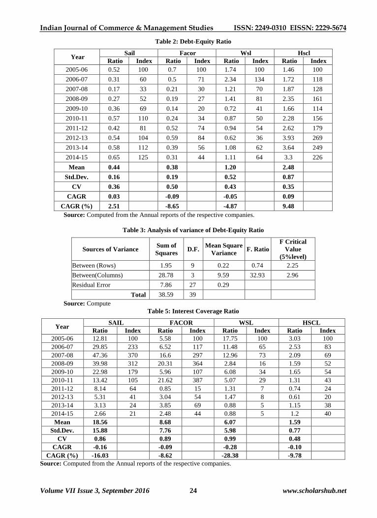
Debt-Equity Ratio:

Debt to equity ratio is a long term solvency ratio that

indicates the soundness of long-term financial policies

of the company. It shows the relation between the

portion of assets provided by the stockholders and the

portion of assets provided by creditors.

The Table 3 showed that the mean debt-equity ratio of

SAIL was 0.44 which is statistically significant. The

CV value further indicated highly fluctuation (0.36) in

this ratio during the study period. Further, debt-equity

ratio of SAIL registered positive (0.03) compound

annual growth rate during the study period.

The mean debt-equity ratio of FACOR was 0.38

which is statistically significant. The CV value further

indicated erratic fluctuation (0.50) in this ratio during

the study period. Further, debt-equity ratio of FACOR

registered negative (-0.09) compound annual growth

rate during the study period.

The mean debt-equity ratio of WSL was 1.20 which is

statistically significant. The CV value further

indicated moderate fluctuation (0.43) in this ratio

during the study period. Further, debt-equity ratio of

WSL registered negative (-0.05) compound annual

compound annual growth rate during the study period.

The mean debt-equity ratio of HSCL was 2.48 which

is statistically significant. The CV value further


during the study period. Further, debt-equity ratio of

WSL registered positive (0.09) compound annual


It is evident from the Table 3 that the debt-equity

ratio only companies has registered better

performance when compared to the standard norm 1:1

during the study period. So, the debt-equity ratio was

better in SAIL and FACOR. Table 3. also indicated

the HSCL had the highest mean debt-equity ratio,

followed by WSL, SAIL and FACOR. The CV value

also indicated that moderate fluctuation in debt-equity

ratio of public sector steel companies during the study

period. The compound annual growth rate of debt-

equity ratio had registered positive value in positive

value in all companies during the study period.

To judge whether the difference in the mean values of

debt-equity ratio between the companies and between

the years during the year period, the following

hypothesis are framed and tested.

H0 – There is no significant difference in debt-equity

ratio between the companies and between years.

It is evident from the Table 4 that the differences

between debt- equity in between the companies are

not significant because the calculated value of „F‟

(0.74) is less than the table value of „F‟ (2.2.25) at the

5 per cent level of significance. Hence, the null

hypothesis is accepted. Further, the difference

between years are significant because the calculated

value of „F‟ (32.93) is more than the table value of „F‟

(2.96) at the 5 percent value of significance and the

null hypothesis is also rejected.

Hence, the financial structure of the selected

companies measured through debt-equity ratio was not

satisfactory and should not be adequate during the

study period.

Interest Coverage Ratio:

The interest coverage ratio calculation shows how

easy it is for a company to pay interest on its

outstanding debt. It also gives you a picture of how far

a company's earnings would have to fall before it was

in danger of defaulting on its debt and is therefore a

good gauge of its short-term health. Most shareholders

look for an interest coverage ratio of at least 1.5. The

fixed interest coverage ratio for the selected public

sector steel companies during the study period

presented.

It is evident from the table 5 that the interest coverage

ratio of SAIL had registered fluctuating trend and

ranged from 12.81 in the year 2005-2006 to 2.66 in

the year 2014-2015 during the study period. The

Table 5 showed that the highest mean interest

coverage ratio of SAIL was 18.56 which is



the study period. Further, interest coverage ratio of

SAIL registered negative (-0.16) compound annual

growth rate during the study period.



The interest coverage ratio of FACOR was registered

fluctuating trend and ranged from 5.58 in the year

2005-2006 to 2.48 in the year 2014- 2015 during the

study period. The Table 5 showed that the mean

interest coverage ratio of FACOR was 8.68 which is



the study period. Further, interest coverage ratio of

FACOR registered negative (-0.09) compound annual


Table 5 also indicated the SAIL had the highest mean

interest coverage ratio, followed by FACOR, WSL

and HSCL. The CV value also indicated that erratic

fluctuation in interest coverage ratio of public sector

steel companies during the study period. The

compound annual growth rate of interest coverage

ratio had registered negative value in all the selected

steel companies during the study period.


interest coverage ratio between the companies and

between the years during the year period, the

following hypothesis are framed and tested.

Ho – There is no significant difference in interest

coverage ratio between the companies and between

years.


between interest coverage in between the companies

are significant because the calculated value of „F‟

(2.53) is more than the table value of „F‟ (2.25) at the

5 percent level of significance. Hence, the null

hypothesis is rejected. Further, the difference between

years are significant because the calculated value of

„F‟ (8.18) is more than the table value of „F‟ (2.96) at

5 percent value of significance and the null hypothesis

is rejected.


companies measured through interest coverage ratio

was not satisfactory and should not be adequate during

the study period.

Analysis of Profitability:

Gross Profit Ratio:

Gross profit ratio (GP ratio) is a profitability ratio that

shows the relationship between gross profit and total

net sales revenue. It is a popular tool to evaluate the

operational performance of the business. Generally, a

higher ratio is considered better.

The Table 7 showed that the mean gross profit ratio of

SAIL was 14.96 which are statistically significant.

The CV value further indicated moderate fluctuation

(0.49) in this ratio during the study period. Further,

gross profit ratio of SAIL registered negative (-0.10)


The mean gross profit ratio of FACOR was 11.00

which is statistically significant. The CV value further


during the study period. Further, gross profit ratio of



The mean gross profit ratio of WSL was 8.48 which

are statistically significant. The CV value further

indicated consistency (0.79) in this ratio during the

study period. Further, gross profit ratio of WSL



The mean gross profit ratio of HSCL was 9.65 which

are statistically significant. The CV value further


study period. Further, gross profit ratio of HSCL

registered positive (0.05) compound annual growth


It is evident the Table 7 that the gross profit ratio all

the selected companies has registered higher

performance during the study period. So, the gross

profit ratio was good during the study period. Table 7

also indicated the SAIL had the highest mean gross

profit ratio, followed by FACOR, HSCL and WSL.

The CV value also indicated that fluctuations in gross

profit ratio of public sector steel companies during the

study period. The compound annual growth rate of

gross profit ratio had registered negative value in

SAIL, FACOR and WSL and positive value in HSCL

during the study period.


Gross Profit Ratio between the companies and


following hypothesis is framed and tested.

H0 – There is no significant difference in Gross Profit



between gross profit ratios in between the companies


(4.22) is more than the table value of „F‟ (2.25) at 5

percent level of significance. Hence, the null



„F‟ (3.79) is higher than the table value of „F‟ (2.96) at


is also rejected.


companies measured through gross profit ratio was

not satisfactory and should not be adequate during the

study period.

Net Profit Ratio:

Net profit ratio (margin) is a key financial indicator

used to assess the profitability of a company that

shows relationship between net profit after tax and net

sales. A low profit margin indicates a low margin of

safety: higher risk that a decline in sales will erase

profits and result in a net loss.



The Table 9 showed that the mean net profit ratio of


CV value further indicated moderate fluctuation (0.62)

in this ratio during the study period. Further, net

profit ratio of SAIL registered negative (-0.11)


The mean net profit ratio of FACOR was 6.45 which

is statistically significant. The CV value further


during the study period. Further, net profit ratio of



The mean net profit ratio of WSL was 4.36 which is



study period. Further, net profit ratio of WSL



The mean net profit ratio of HSCL was 1.75 which is



study period. Further, net profit ratio of HSCL



It is evident the Table 9 that the net profit ratio all the

selected companies has registered lesser performance

during the study period except SAIL and FACOR. So,

the net profit ratio was poor during the study period.

Table 5 also indicated the SAIL had the highest mean

net profit ratio, followed by FACOR, WSL and

HSCL. The CV value also indicated that fluctuations

in net profit ratio of public sector steel companies

during the study period. The compound annual

growth rate of net profit ratio had registered negative

values in all the companies during the study period.


Net Profit Ratio between the companies and between

the years during the year period, the following

hypothesis is framed and tested.

H0 – There is no significant difference in Net Profit



between net profit ratios in between the companies are

significant because the calculated value of „F‟ (3.74) is

more than the table value of „F‟ (2.25) at 5 percent level

of significance. Hence, the null hypothesis is rejected.

Further, the difference between years are significant

because the calculated value of „F‟ (10.21) is higher

than the table value of „F‟ (2.96) at 5 percent value of

significance and the null hypothesis is also rejected.


companies measured through net profit ratio was not


study period.

Return on Capital Employed:

Return on capital employed (ROCE) is a profitability

ratio that measures how efficiently a company can

generate profits from its capital employed by

comparing net operating profit to capital employed.

ROCE is a long-term profitability ratio because it

shows how effectively assets are performing while

taking into consideration long-term financing. Higher

the ratio performance of the companies is effective or

satisfactory.

It is evident from the table 11 that the return on capital

employed ratio of SAIL had registered fluctuating

trend and ranged from 35.8 in the year 2005-2006 to

5.6 in the year 2014-2015 during the study period.

The Table 11 showed that the highest mean return on

capital employed ratio of SAIL was 21.15 which is



the study period. Further, return on capital employed

ratio of SAIL registered negative (-0.19) compound


The return on capital employed ratio of FACOR was

registered fluctuating trend and ranged from 13.28 in

the year 2005-2006 to 12.09 in the year 2014- 2015

during the study period. The Table 11 showed that the

mean return on capital employed ratio of FACOR was

20.60 which is statistically significant. The CV value

further indicated erratic fluctuation (0.70) in this ratio

during the study period. Further, return on capital

employed ratio of FACOR registered negative (-0.01)


The return on capital employed ratio of WSL was




mean return on capital employed ratio of WSL was




employed ratio of WSL registered negative (-0.15)


The return on capital employed ratio of HSCL was

registered fluctuating trend and ranged from 6.7 in the

year 2005-2006 to 13.03 in the year 2014- 2015


mean return on capital employed ratio of HSCL was




employed ratio of HSCL registered positive (0.08)


Table 11 also indicated the SAIL had the highest

mean return on capital employed ratio, followed by,

FACOR, WSL and HSCL. The CV value also

indicated that erratic fluctuation in return on capital

employed ratio of public sector steel companies

during the study period. The compound annual growth

rate of return on capital employed ratio had registered



negative values in all the selected steel companies

during the study period except HSCL.


return on capital employed ratio between the

companies and between the years during the year

period, the following hypothesis is framed and tested.

Ho – There is no significant difference in Return on

Capital Employed Ratio between the companies and

between years.


between return on capital employed in between the

companies are significant because the calculated value

of „F‟ (3.17) is more than the table value of „F‟ (2.25)

at 5 percent level of significance. Hence, the null





is rejected.


companies measured through return on capital

employed ratio was not satisfactory and should not be

adequate during the study period.

Return on Net worth:

Return on Net Worth (RONW) is used in finance as a

measure of a company‟s profitability. It reveals how

much profit a company generates with the money that

the equity shareholders have invested. RONW is a

measure for judging the returns that a shareholder gets

on his investment.

It is evident from the table 13 that the return on net

worth ratio of SAIL had registered fluctuating trend

and ranged from 32.64 in the year 2005-2006 to 4.88

in the year 2014-2015 during the study period. The

Table 13 showed that the highest mean return on net

worth ratio of SAIL was 18.27 which are statistically

significant. The CV value further indicated erratic

fluctuation (0.67) in this ratio during the study period.

Further, return on net worth ratio of SAIL registered

negative (-0.19) compound annual growth rate during

the study period.

The return on net worth ratio of FACOR was




mean return on net worth ratio of FACOR was 12.02

which are statistically significant. The CV value


during the study period. Further, return on net worth

ratio of FACOR registered negative (-0.08) compound


The return on net worth ratio of WSL was registered


2005-2006 to -0.84 in the year 2014- 2015 during the


return on net worth ratio of WSL was 10.61 which are



the study period. Further, return on net worth ratio of

WSL registered negative (-1.74) compound annual


The return on net worth ratio of HSCL was registered


2005-2006 to 5.88 in the year 2014- 2015 during the


return on net worth ratio of HSCL was 3.99 which is



the study period. Further, return on net worth ratio of

HSCL registered negative (-0.09) compound annual


Table 13 also indicated the SAIL had the highest

mean return on net worth ratio, followed by, FACOR,

WSL and HSCL. The CV value also indicated that

erratic fluctuation in return on net worth ratio of

public sector steel companies during the study period.

The compound annual growth rate of return on capital

employed ratio had registered negative values in all

the selected steel companies during the study period.


return on net worth ratio between the companies and



Ho – There is no significant difference in Return on

Net Worth Ratio between the companies and between

years.


between return on net worth in between the companies








is rejected.


companies measured through return on net worth ratio

was not satisfactory and should not be adequate during

the study period.

Analysis of Efficiency:

Investment Turnover Ratio:

Higher investment turnover ratios equate to more

efficient companies. The investment turnover ratio

tells the investor-analyst how effectively a company

uses its resources to generate revenues.

The Table 15 showed that the mean investment

turnover ratio of SAIL was 4.55 which is statistically

significant. The CV value further indicated moderate


Further, investment turnover ratio of SAIL registered


the study period.



The mean investment turnover ratio of FACOR was


further indicated moderate fluctuation (0.23) in this

ratio during the study period. Further, investment

turnover ratio of FACOR registered negative (-0.05)


The mean investment turnover ratio of WSL was 5.02

which is statistically significant. The CV value

further indicated consistency (0.38) in this ratio during

the study period. Further, investment turnover ratio of

WSL registered negative (0.06) compound annual


The mean investment turnover ratio of HSCL was


further indicated consistency (0.21) in this ratio during

the study period. Further, investment turnover ratio of

HSCL registered negative (-0.04) compound annual


It is evident the Table 15 that the investment turnover

ratio all the selected companies has registered lesser

performance during the study period. So the investment

turnover ratio was poor during the study period. Table

15 also indicated the FACOR had the highest mean

investment turnover ratio, followed by WSL, SAIL and

HSCL. The CV value also indicated that fluctuations in

investment turnover ratio of public sector steel

companies during the study period. The compound

annual growth rate of investment turnover ratio had

registered negative values in three companies and WSL

registered positive during the study period.


Investment Turnover Ratio between the companies

and between the years during the year period, the


H0 – There is no significant difference in Investment

Turnover Ratio between the companies and between years


between investment turnover ratio in between the

companies are not significant because the calculated

value of „F‟ (1.38) is less than the table value of „F‟

(2.25) at 5 percent level of significance. Hence, the

null hypothesis is accepted. Further, the difference


value of „F‟ (26.12) is higher than that the table value

of „F‟ (2.96) at 5 percent value of significance and the

null hypothesis is rejected.


companies measured through investment turnover

ratio satisfactory and should be adequate during the

study period.

Fixed Assets Turnover Ratio:

The fixed-assets turnover ratio measures a company's

ability to generate net sales from fixed asset investments

– specially property, land and equipment (PP&E)- net of

depreciation. A higher fixed-assets turnover ratio shows

that the company has been more effective.

It is evident from the table 17 that the fixed assets

turnover ratio of SAIL had registered constant trend

and ranged from 0.95 in the year 2005-2006 to 0.7 in

the year 2014-2015 during the study period. The

Table 17 showed that the lowest mean fixed assets

turnover ratio of SAIL was 1.06 which is statistically

not significant. The CV value further indicated erratic


Further, fixed assets turnover ratio of SAIL registered


the study period.

The fixed assets turnover ratio of FACOR was



during the study period. The Table15 showed that the

mean fixed assets turnover ratio of FACOR was 3.75

which is statistically significant. The CV value


during the study period. Further, fixed assets turnover

ratio of FACOR registered negative (-0.07)


Table 17 also indicated the FACOR had the highest

mean interest coverage ratio, followed by, HSCL,

WSL and SAIL. The CV value also indicated that

erratic fluctuation in fixed assets turnover ratio of

public sector steel companies during the study period.

The compound annual growth rate of fixed assets

turnover ratio had registered negative values in all the

selected steel companies during the study period.


fixed assets turnover ratio between the companies and



Ho – There is no significant difference in Fixed

Assets Turnover Ratio between the companies and

between years


between fixed assets turnover in between the

companies are not significant because the calculated

value of „F‟ (1.47) is less than the table value of „F‟

(2.25) at 5 percent level of significance. Hence, the

null hypothesis is accepted. Further, the difference


value of „F‟ (19.56) is more than the table value of „F‟

(2.96) at 5 percent value of significance and the null

hypothesis is rejected.


companies measured through fixed assets turnover

ratio was not satisfactory and should not be adequate

during the study period.

Analysis of Short-term Solvency (Liquidity):

Current Ratio:

The management of working capital involves decisions

about the amount and composition current assets and



how they are financed. Such decisions involve a trade-off

between solvency and profitability. In inter-firm

comparison, the firm with higher current ratio has better

liquidity. Therefore, current ratio is used to explain

profitability of Indian steel manufacturing companies.

The current ratio for the selected public sector companies

during the study period presented in Table 19.

The Table 19 showed that the mean current ratio of


CV value further indicated consistency (0.50) in this

ratio during the study period. Further, current ratio of

SAIL registered negative (-0.07) compound annual


The mean current ratio of FACOR was 1.24 which is



study period. Further, current ratio of FACOR



The mean current ratio of WSL was 0.94 which is

statistically significant. The CV value further indicated

consistency (0.19) in this ratio during the study period.

Further, current ratio of WSL registered zero (0.00)


The mean current ratio of HSCL was 1.44 which is



study period. Further, current ratio of HSCL registered


the study period.

It is evident from the Table 19 that the current ratio of

all the four companies had registered lower

performance when compared to the standard norm

2:1.So, the current ratio was poor during the study

period. Table1 also indicated the HSCL had the

highest mean current ratio, followed by FACOR,

SAIL and WSL. The CV value also indicated that the

fluctuation in current ratio of public sector steel

companies during the study period. The compound

annual growth rate of current ratio had registered

negative value in three selected steel companies and

one company zero during the study period.

To judge whether the different in the mean values of

current into between the companies and between the

years during the year period, the following hypothesis

is framed and tested.

H0 – There is no significant difference in current ratio

between the companies and between years.


between current ratio in between the companies are

not significant because the calculated value of „F‟





„F‟ (3.57) is higher than the table value of „F‟ (2.96) at


is also rejected.


companies measured through current ratio was not


study period.

Quick Ratio:

The current ratio is not a sufficient indicator of the

weakness or soundness of the liquidity of a company.

The important question is whether the current assets

are held in liquid from or not. If working capital is

tied up in inventories and prepaid expenses, which

cannot be converted promptly into cast, the company

may be unable to honor its obligations for want of

cash funds. Therefore, the solvency of a company can

be better judged by quick ratio. The quick ratio is an

important device for judging the liquidity position of a

business. The liquidity ratio for the selected public

sector steel companies during the study period

presented in Table 21.

The Table 21 showed that the mean quick ratio of


CV value further indicated moderate fluctuation (0.52)

in this ratio during the study period. Further, quick

ratio of SAIL registered negative (-0.04) compound


The mean quick ratio of FACOR was 1.08 which is



during the study period. Further, quick ratio of



The mean quick ratio of WSL was 0.75 which is



study period. Further, quick ratio of WSL registered

zero (0.00) compound annual growth rate during the

study period.

The mean quick ratio of HSCL was 0.84 which is



study period. Further, quick ratio of HSCL registered


the study period.

It is evident the Table 21 that the quick ratio all the

selected companies has registered lower performance

except FACOR when compared to the standard norm

1:1 during the study period. So, the quick ratio was

poor during the study period. Table 21 also indicated

the FACOR had the highest mean quick ratio,

followed by SAIL, HSCL and WSL. The CV value

also indicated that consistency in quick ratio of public

sector steel companies during the study period. The

compound annual growth rate of quick ratio had

registered negative value in SAIL, FACOR and HSCL

and zero value in WSL during the study period.


Quick Ratio between the companies and between the



years during the year period, the following hypothesis

is framed and tested.

H0 – There is no significant difference in Quick Ratio

between the companies and between years


between quick ratios in between the companies are not

significant because the calculated value of „F‟ (0.60) is

less than the table value of „F‟ (2.25) at 5 percent level

of significance. Hence, the null hypothesis is accepted.

Further, the difference between years are not significant

because the calculated value of „F‟ (1.30) is lesser that

the table value of „F‟ (2.96) at 5 percent value of

significance and the null hypothesis is also accepted.

Hence, the financial structure of the selected companies

measured through quick ratio was satisfactory and

should be adequate during the study period.

Conclusion:

The analysis of Production, Sales and Profit of the

selected steel manufacturing companies indicates

average performance during the study period. The

analysis of solvency of selected steel companies

showed the poor solvency position. The analysis of

profitability of selected steel companies showed the

efficiency of Steel Companies in not utilizing their

resources effectively in generating their return.

However, the selected companies should improve

their Liquidity position. It is high time that the

authorities and the government also need to give due

attention to the financial viability of public sector steel

manufacturing companies. Finally it is concluded that

the selected companies could re-frame their optimum

capital structure, capacity utilization and liquidity

position for enhancing the further profitability in

future.

References:

1. Jagan Mohan Rao, P. (1993). Financial Appraisal

of Indian Automotive Tyre Industry, Finance

India, Vol.VII, No.3, pp.683-685.

2. Kallu Rao, P. (1993). Inter Company Financial

Analysis of Tea Industry Retrospect and Prospect,

Finance India, Vol. VII, No.3, pp.587-602.

3. Pai V.S, Vadivel.V and Kamala K.H. (Dec 1995).

„Diversified companies and financial

performance: A study, Finance India, Vol.IX,

No.4, pp. 977-988.

4. Vijayakumar, A. (1996), Asessment of Corporate

Liquidity – A Discriminant Analysis approach,

The Management Accountant, Vol.31, No.8,

pp.589-591.

5. Key Sengupta (1998). An empirical exploration

of the performance of Fertilizers Industry in

India: An econometric analysis, Artha Vijnana,

Vol.XL, No.3, pp.252-262.

6. Raghunathan V. and Prabina Das, (1999).

Corporate Performance: Post-Liberalization, The

ICFAI Journal of Applied Finance, Vol.5, No.2,

pp.6- 29.

7. Rajeswari (2000). Liquidity Management of

Tamil Nadu Cement Corporation Ltd,

Alangulam- A Case Study, The Management

Accountant, Vol.II, No.2, pp. 377-378.

8. Aggarwal, N. and Singla, S.K. (2001). How to

develop a single index for financial performance,

Indian Management, Vol.12, No.5, pp.59-62.

9. Dabasish Sur (2001). Liquidity Management: An

overview of four companies in Indian Power

Sector, The Management Accountant, pp.407-412.

10. Mansur, A. and Mulla, (2002). Use of „Z‟ score

analysis for evaluation of financial health of

textile mills – A case study, Abhigyan, Vol.XIX,

No.4, pp.37-40.

11. Sudarsana Reddy, G. (2003). Financial

Performance of Paper industry in A.P, Finance

India, Vol. XVII, No.3, pp. 1027-1033.

12. Ram Kumar Kakani, Biswatosh Saha and Reddy,

V.N. (2003). Determinants of financial

performance of India corporate sector in the post-

liberalization era; an exploratory study, NSE

Research Initiative, Paper No: 5, National Stock

Exchange of India Limited, pp. 1-38.

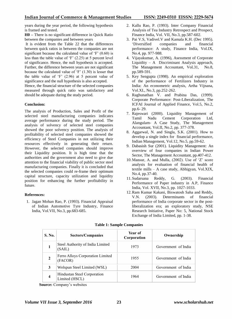
Table 1: Sample Companies

S. No. Sectors/Companies Year of

Corporation Ownership

1 Steel Authority of India Limited

(SAIL) 1973 Government of India

2 Ferro Alloys Corporation Limited

(FACOR) 1955 Government of India

3 Welspun Steel Limited (WSL) 2004 Government of India

4 Hindustan Steel Corporation

Limited (HSCL) 1964 Government of India

Source: Company‟s websites



Table 2: Debt-Equity Ratio

Year Sail Facor Wsl Hscl

Ratio Index Ratio Index Ratio Index Ratio Index

2005-06 0.52 100 0.7 100 1.74 100 1.46 100

2006-07 0.31 60 0.5 71 2.34 134 1.72 118

2007-08 0.17 33 0.21 30 1.21 70 1.87 128

2008-09 0.27 52 0.19 27 1.41 81 2.35 161

2009-10 0.36 69 0.14 20 0.72 41 1.66 114

2010-11 0.57 110 0.24 34 0.87 50 2.28 156

2011-12 0.42 81 0.52 74 0.94 54 2.62 179

2012-13 0.54 104 0.59 84 0.62 36 3.93 269

2013-14 0.58 112 0.39 56 1.08 62 3.64 249

2014-15 0.65 125 0.31 44 1.11 64 3.3 226

Mean 0.44 0.38 1.20 2.48

Std.Dev. 0.16 0.19 0.52 0.87

CV 0.36 0.50 0.43 0.35

CAGR 0.03 -0.09 -0.05 0.09

CAGR (%) 2.51 -8.65 -4.87 9.48

Source: Computed from the Annual reports of the respective companies.

Table 3: Analysis of variance of Debt-Equity Ratio

Sources of Variance Sum of

Squares D.F.

Mean Square

Variance F. Ratio

F Critical

Value

(5%level)

Between (Rows) 1.95 9 0.22 0.74 2.25

Between(Columns) 28.78 3 9.59 32.93 2.96

Residual Error 7.86 27 0.29

Total 38.59 39

Source: Compute

Table 5: Interest Coverage Ratio

Year SAIL FACOR WSL HSCL


2005-06 12.81 100 5.58 100 17.75 100 3.03 100

2006-07 29.85 233 6.52 117 11.48 65 2.53 83

2007-08 47.36 370 16.6 297 12.96 73 2.09 69

2008-09 39.98 312 20.31 364 2.84 16 1.59 52

2009-10 22.98 179 5.96 107 6.08 34 1.65 54

2010-11 13.42 105 21.62 387 5.07 29 1.31 43

2011-12 8.14 64 0.85 15 1.31 7 0.74 24

2012-13 5.31 41 3.04 54 1.47 8 0.61 20

2013-14 3.13 24 3.85 69 0.88 5 1.15 38

2014-15 2.66 21 2.48 44 0.88 5 1.2 40

Mean 18.56 8.68 6.07 1.59

Std.Dev. 15.88 7.76 5.98 0.77

CV 0.86 0.89 0.99 0.48

CAGR -0.16 -0.09 -0.28 -0.10

CAGR (%) -16.03 -8.62 -28.38 -9.78




Table 6: Analysis of Variance of Interest Coverage Ratio

Sources of Variance

Sum of

Squares D.F.

Mean Square

Variance

F. Ratio

F Critical Value

(5%level)

Between (Rows) 1435.75 9 159.53 2.53 2.25

Between(Columns) 1547.54 3 515.85 8.18 2.96


Total 4686.909 39

Source: Computed

Table 7: Gross Profit Ratio



2005-06 17.94 100 14.03 100 16.25 100 9.93 100

2006-07 24.82 138 16.6 118 14.6 90 7.86 79

2007-08 25.3 141 24.58 175 15.18 93 10.33 104

2008-09 17.62 98 15.3 109 8.19 50 9.75 98

2009-10 20.3 113 4.81 34 15.21 94 9.48 95

2010-11 13.55 76 10.59 75 10.22 63 9.51 96

2011-12 10.13 56 1.31 9 1.8 11 7.09 71

2012-13 7.87 44 7.86 56 2.11 13 5.23 53

2013-14 5.32 30 8.65 62 0.44 3 12 121

2014-15 6.75 38 6.24 44 0.8 5 15.27 154

Mean 14.96 11.00 8.48 9.65

Std.Dev. 7.34 6.78 6.67 2.73

CV 0.49 0.62 0.79 0.28

CAGR -0.10 -0.09 -0.28 0.05

CAGR

(%) -10.29 -8.61 -28.44 4.90


Table 8: Analysis of variance of Gross Profit ratio


Squares D.F.

Mean Square

Variance

F. Ratio

F Critical Value

(5%level)

Between (Rows) 798.09 9 88.68 4.22 2.25

Between(Columns) 238.66 3 79.55 3.79 2.96


Total 1604.00 39

Source: Computed

Table 9: Net Profit Ratio

Year SAIL FERROW WELSPUM HINDUSTAN


2005-06 13.76 100 7.76 100 3.33 100 8.22 100

2006-07 17.53 127 8.17 105 5.31 159 3.27 40

2007-08 18.26 133 15.75 203 8.7 261 3.47 42

2008-09 14.25 104 9.17 118 3.93 118 3.74 45

2009-10 16.77 122 3.96 51 8.09 243 2.22 27

2010-11 0 0 7.57 98 5.81 174 1.73 21

2011-12 7.7 56 -0.69 -9 1.12 34 -5.57 -68

2012-13 5.16 38 4.82 62 8 240 -3.59 -44



Year SAIL FERROW WELSPUM HINDUSTAN


2013-14 5.62 41 4.81 62 -0.36 -11 1.99 24

2014-15 4.69 34 3.16 41 -0.31 -9 1.97 24

Mean 10.37 6.45 4.36 1.75

Std.Dev. 6.48 4.39 3.41 3.85

CV 0.62 0.68 0.78 2.21

CAGR -0.11 -0.10 -1.77 -0.15

CAGR (%) -11.27 -9.50 -176.81 -14.68


Table 10: Analysis of variance of Net Profit Ratio


Squares D.F.

Mean Square

Variance

F. Ratio

F Critical Value

(5%level)

Between (Rows) 437.96 9 48.66 3.74 2.25

Between(Columns) 398.34 3 132.78 10.21 2.96


Total 1187.51 39

Source: Computed

Table 11: Return on Capital Employed



2005-06 35.8 100 13.28 100 21.47 100 6.7 100

2006-07 44.13 123 23.59 178 17.4 81 8.62 129

2007-08 42.76 119 55.21 416 19.19 89 11.57 173

2008-09 26.92 75 29 218 15.27 71 10.73 160

2009-10 20.29 57 10.36 78 22.51 105 9.24 138

2010-11 13.03 36 26.81 202 12.61 59 8.55 128

2011-12 11.06 31 4.26 32 4.64 22 8.28 124

2012-13 7.03 20 13.96 105 6.18 29 5.58 83

2013-14 4.84 14 17.42 131 4.84 23 12.03 180

2014-15 5.6 16 12.09 91 4.75 22 13.03 194

Mean 21.15 20.60 12.89 9.43

Std.Dev. 15.34 14.41 7.27 2.38

CV 0.73 0.70 0.56 0.25

CAGR -0.19 -0.01 -0.15 0.08

CAGR (%) -18.63 -1.04 -15.43 7.67




Table 12: Analysis of variance of Return on Capital Employed Ratio

Sources of Variance

Sum of

Squares D.F.

Mean Square

Variance

F. Ratio

F Critical Value

(5%level)

Between (Rows) 2317.62 9 257.51 3.17 2.25

Between(Columns) 1004.44 3 334.81 4.12 2.96


Total 5518.22 39

Source: Computed

Table 13: Return on Networth



2005-06 32.64 100 16.16 100 12.23 100 14.03 100

2006-07 36.1 111 19.17 119 21.82 178 8.76 62

2007-08 32.7 100 4.76 29 23.59 193 10.99 78

2008-09 22.1 68 19.86 123 15.12 124 12.66 90

2009-10 20.29 62 9.12 56 19.66 161 5.36 38

2010-11 13.34 41 20.15 125 11.91 97 4.66 33

2011-12 8.92 27 -1.86 -12 1.8 15 -17.09 -122

2012-13 5.59 17 12.39 77 1.2 10 -11.83 -84

2013-14 6.12 19 13.09 81 -0.39 -3 6.46 46

2014-15 4.88 15 7.37 46 -0.84 -7 5.88 42

Mean 18.27 12.02 10.61 3.99

Std.Dev. 12.25 7.25 9.54 10.30

CV 0.67 0.60 0.90 2.58

CAGR -0.19 -0.08 -1.74 -0.09

CAGR

(%) -19.04 -8.35 -174.26 -9.21


Table 14: Analysis of variance of Return on Capital Employed Ratio


Squares D.F.

Mean Square

Variance

F. Ratio

F Critical Value

(5%level)

Between (Rows) 2359.41 9 262.16 5.72 2.25

Between(Columns) 1029.90 3 343.30 7.49 2.96


Total 4626.53 39

Source: Computed



Table 15: Investment Turnover Ratio



2005-06 5.22 100 11.55 100 3.72 100 1.62 100

2006-07 7.43 142 11.45 99 5.89 158 1.67 103

2007-08 8.58 164 9.57 83 3.34 90 1.73 107

2008-09 5.84 112 7.8 68 2.71 73 1.33 82

2009-10 6.01 115 6.71 58 5.67 152 1.1 68

2010-11 0 0 6.8 59 5.45 147 0.97 60

2011-12 3.36 64 6.37 55 3.5 94 1.17 72

2012-13 3.13 60 7.35 64 4.5 121 1.04 64

2013-14 3.07 59 8.04 70 9.2 247 1.23 76

2014-15 2.87 55 7.39 64 6.19 166 1.16 72

Mean 4.55 8.30 5.02 1.30

Std.Dev. 2.54 1.90 1.90 0.28

CV 0.56 0.23 0.38 0.21

CAGR -0.06 -0.05 0.06 -0.04

CAGR

(%) -6.43 -4.84 5.82 -3.64


Table 16: Analysis of variance of Investment Turnover Ratio


Squares D.F.

Mean Square

Variance

F. Ratio

F Critical Value

(5%level)

Between (Rows) 39.09 9 4.34 1.38 2.25

Between(Columns) 246.16 3 82.05 26.12 2.96


Total 370.05 39

Source: Computed

Table 17: Fixed assets turnover ratio



2005-06 0.95 100 5.99 100 2.37 100 2.91 100

2006-07 1.13 119 6.83 114 2.02 85 2.2 76

2007-08 1.28 135 4.44 74 1.79 76 2.23 77

2008-09 1.33 140 1.81 30 2.22 94 1.99 68

2009-10 1.14 120 1.79 30 2.24 95 2.02 69

2010-11 1.1 116 3.28 55 2 84 2.08 71

2011-12 1.1 116 3.19 53 1.49 63 1.96 67

2012-13 1.04 109 3.31 55 1.65 70 1.88 65

2013-14 0.86 91 3.61 60 1.15 49 2.02 69

2014-15 0.7 74 3.25 54 1.14 48 2.08 71

Mean 1.06 3.75 1.81 2.14

Std.Dev. 0.19 1.62 0.44 0.29

CV 0.18 0.43 0.24 0.14

CAGR -0.03 -0.07 -0.08 -0.04

CAGR (%) -3.34 -6.57 -7.81 -3.66




Table 18: Analysis of variance of Fixed Assets Turnover Ratio


Squares D.F.

Mean Square

Variance

F. Ratio

F Critical Value

(5%level)

Between (Rows) 8.69 9 0.97 1.47 2.25

Between(Columns) 38.53 3 12.84 19.56 2.96


Total 64.96 39

Source: Computed

Table 19: Current ratio



2005-06 1.29 100 1.32 100 0.92 100 2.15 100

2006-07 1.58 122 1.49 113 1.32 143 1.75 81

2007-08 1.71 133 2.18 165 0.94 102 1.49 69

2008-09 1.75 136 1.87 142 0.87 95 1.59 74

2009-10 2.03 157 1.41 107 1.06 115 1.55 72

2010-11 0 0 1.22 92 0.81 88 1.4 65

2011-12 1.2 93 0.85 64 0.94 102 0.97 45

2012-13 1.02 79 0.7 53 1.02 111 1.27 59

2013-14 0.79 61 0.72 55 0.64 70 1.19 55

2014-15 0.68 53 0.67 51 0.91 99 1.08 50

Mean 1.21 1.24 0.94 1.44

Std.Dev. 0.61 0.52 0.18 0.35

CV 0.50 0.42 0.19 0.24

CAGR -0.07 -0.07 0.00 -0.07

CAGR (%) -6.87 -7.26 -0.12 -7.36


Table 20: Analysis of variance of Current Ratio


Squares D.F.

Mean Square

Variance

F.

Ratio

F Critical Value

(5%level)

Between (Rows) 3.88 9 0.43 3.63 2.25

Between(Columns) 1.27 3 0.42 3.57 2.96


Total

Source: Computed



Table 21: Quick Ratio



2005-06 0.78 100 1.06 100 0.75 100 1.41 100

2006-07 1.11 142 1.25 118 0.99 132 0.58 41

2007-08 1.31 168 1.62 153 0.62 83 0.48 34

2008-09 1.25 160 1.75 165 0.64 85 0.4 28

2009-10 1.61 206 1.09 103 1.13 151 0.47 33

2010-11 0 0 1.04 98 0.81 108 0.56 40

2011-12 0.82 105 0.7 66 0.67 89 0.78 55

2012-13 0.7 90 1.03 97 0.65 87 1.16 82

2013-14 0.63 81 0.77 73 0.47 63 1.32 94

2014-15 0.56 72 0.52 49 0.75 100 1.25 89

Mean 0.88 1.08 0.75 0.84

Std.Dev. 0.46 0.38 0.19 0.40

CV 0.52 0.35 0.26 0.47

CAGR -0.04 -0.08 0.00 -0.01

Source: Computed from the Annual reports of the respective companies

Table 22: Analysis of variance of Quick ratio


Squares D.F.

Mean Square

Variance

F.

Ratio

F Critical Value

(5%level)

Between (Rows) 0.84 9 0.09 0.60 2.25

Between(Columns) 0.59 3 0.19 1.30 2.96


Total 5.58 39

Source: Computed

******

SPEL ANALYSIS OF FINANCIAL STATEMENTS OF ...scholarshub.net/ijcms/vol7/issue3/Paper_03.pdfIndian...

Documents

Transcript of SPEL ANALYSIS OF FINANCIAL STATEMENTS OF ...scholarshub.net/ijcms/vol7/issue3/Paper_03.pdfIndian...